Advanced Optimization of Source Power Delivery for Transmission Loss Reduction—Case Study

Abstract

The article presents the development and laboratory validation of a current optimization algorithm designed for voltage-source systems. The algorithm was implemented in a real laboratory setup using a synchronous generator driven by a DC motor to model a fragment of a power system. During tests, transient states were intentionally inducted to evaluate the algorithm’s performance. The proposed optimization method effectively reduced instantaneous current peaks by over 60% and the overall RMS current by approximately 4%, leading to lower power losses and decreased conductor temperatures. These improvements resulted in nearly 8% minimization of power losses and a noticeable reduction in heat generation during transient and fault conditions. The solution is particularly suitable for islanded networks with renewable and unstable energy sources.

1. Introduction

The architecture of modern power systems is undergoing rapid and profound transformation. Three dominant trends are driving this evolution: the large-scale integration of renewable and distributed energy resources (DERs), the widespread penetration of power electronic interfaces, and the diversification of consumer loads [1,2]. While these changes enable greater flexibility, sustainability and decentralization, they also introduce a new set of challenges for network operators [3]. Unlike traditional power systems, which were largely centralized, dominated by linear loads and well-approximated by steady-state sinusoidal assumptions, today’s grids are characterized by rapid fluctuations, stochastic disturbances and widespread nonlinearities [4,5].

A central consequence of these changes is the deterioration of power quality. Distorted voltage and current waveforms, unbalances and elevated harmonics content are increasingly common phenomena [6]. Non-linear loads such as variable speed drives, rectifiers and consumer electronics, as well as renewable generation units interfaced through power converters, introduce not only the useful active component of power but also significant amounts of reactive and distortion power [7,8]. These non-active components circulate within the system without performing useful work, causing additional Joule losses, overloading conductors and transformers, and reducing overall energy efficiency [9,10]. The impact of these effects becomes particularly severe during transient operating conditions (including sudden load switching, voltage dips, intermittent renewable generation and short-duration faults) where the interaction between source and load frequently deviates from its optimal point of operation [11,12]. Under such circumstances, effective energy delivery efficiency can drop well below 80%, despite apparent compliance with long-term voltage quality standards such as EN50160 [13].

Conventional approaches to improving power quality, such as passive filters, shunt and series active filters, and hybrid filter configurations, have achieved partial success in mitigating harmonics and correcting power factor under stationary conditions [14,15]. However, the highly variable and dynamic character of modern networks demands strategies that extend beyond static solutions. In particular, compensation and control schemes must be capable of responding adaptively to rapidly changing conditions, ensuring both high power quality and efficient energy transfer. Advanced approaches have therefore emerged, based on model predictive control (e.g., realized by three-level active power filter [16], constrained finite control set current controller [17], deep learning based active filter [18] or sliding mode control [19]), instantaneous power theories (e.g., realized by dividing the current into active and non-active components [20], FDB-method [21], instantaneous reactive power compensator [22] or reactive power compensators and active power filters for harmonic compensation [23]) and adaptive or data-driven optimization frameworks (e.g., optimal power flow using ant colony optimization [24], improved memetic algorithm [25], multiband power system stabilizers [26], transient stability calculation method [27], emerging techniques such as neural networks, fuzzy logic systems, machine learning [28] or AI [29]). These methods enable real-time adjustment of compensation devices such as active filters or unified power quality conditioners (UPQC), maintaining low total harmonic distortion (THD), stable voltage profiles, and reduced RMS source current even under distorted or fluctuating supply conditions.

Despite these advances, a significant gap remains in the treatment of transient states. Many existing optimization frameworks are designed for steady-state or quasi-stationary operation, and their performance deteriorates when confronted with fast-changing disturbances. This often leads to overcompensation, redundant energy circulation, and increased operational costs. Moreover, while distortion reduction and power factor correction are well-established objectives, comparatively less attention has been devoted to explicitly optimizing the transfer of active power during transient conditions. A comprehensive approach must therefore extend beyond harmonic mitigation to include the fundamental problem of source-load cooperation—delivering the required active power with minimal RMS current and minimal losses.

Formally, this objective can be expressed through optimization criteria such as:

$$\min I_{RMS}\mathrm{subject} \mathrm{to} P\left(t\right)=P^{*}\left(t\right)$$

(1)

where $I_{RMS}$ denotes the root mean square value of the source current, and $P^{*}\left(t\right)$ represents the desired transient active power delivered to the load. This formulation captures the essence of optimal energy transfer under dynamic conditions: ensuring the required level of active power delivery while simultaneously reducing unnecessary circulation of non-active power components. Extending such mathematical descriptions requires introducing transient operators and redefining the concept of active power beyond its classical steady-state formulations. While Fryze’s minimum current approach and Akagi’s instantaneous p-q theory [22,23] provide useful foundations, they require adaptation to accurately describe and optimize energy flow in highly non-stationary, distorted, or unbalanced conditions [30,31].

Recent developments in digital twin technology and hardware-in-the-loop (HIL) testing provide powerful tools for addressing this challenge. Digital twins allow transient-aware algorithms to be tested under realistic scenarios, accounting for non-linearities, stochastic disturbances, and switching phenomena that are sometimes neglected in analytical studies. HIL environments further bridge the gap between simulation and real-world deployment, enabling verification of proposed optimization methods under conditions that closely replicate actual grid disturbances. This combined approach of mathematical modeling, real-time optimization, and experimental validation is essential for ensuring that novel strategies are not only theoretically rigorous but also practically viable.

The present paper builds on these advanced approaches by proposing a novel optimization framework for active power delivery during transient states in modern electrical networks. The contributions of this work are threefold. First, it describes a theoretical extension by formulating a transient definition of active power, supported by operator-based representations that capture dynamic, non-sinusoidal, and distorted conditions. Second, it derives and solves two optimization criteria specially tailored for transient states: the maximization of active power delivery and the minimization of RMS source current subject to active power constraints. Finally, the proposed framework is validated through simulation studies and hardware-in-the-loop experiments, with performance assessed under representative scenarios such as voltage dips, waveform distortions, and load switching events. The results show that explicitly considering transient dynamics in optimization significantly improves the efficiency and resilience of energy transfer. By reducing RMS current, stabilizing voltage profiles, and lowering transmission losses, the proposed method enhances overall system performance and ensures high power quality in the increasingly complex and dynamic environment of modern power systems.

By extending optimization methods and algorithms to power networks and performing appropriate optimization, it is possible to significantly reduce thermal losses in transmission lines, especially under transient and fault conditions, which frequently occur in such networks (short-circuits, voltage sags, overvoltages, and similar disturbances). Optimization of load current contributes to the reduction in thermal losses (increasing the efficiency of electric power transmission). While in steady-state conditions the effectiveness of such optimization is not very high, under fault conditions it already allows for a significant reduction in the Joule thermal integral.

This translates into a reduction in active power losses but, more importantly, during disturbance processes, into lowering the operating temperature of the conductor core in transmission cables/lines. This may indirectly increase the short-circuit withstand capability as a result of lowering the thermal stress during fault states compared to systems without optimization algorithms. Consequently, it may allow for reducing conductor cross-sections when their sizing is dictated primarily by short-circuit withstand conditions, thereby reducing investment costs.

This article presents laboratory test results aimed at demonstrating the influence of an optimization system on reducing the operating temperature of the conductor in a transmission line, compared to the temperature of the same conductor in a non-optimized system, using deliberately induced voltage sags associated with a large change in the load of a laboratory model of a fragment of a power system.

Works such as [32,33] show that despite the high complexity of the algorithms and the advanced theoretical approach, the lack of laboratory validation limits their practical applicability. In this context, our work adds value by implementing a real-time current optimization method under laboratory conditions, while also taking into account hardware constraints and dynamic disturbances.

This paper is organized as follows: Section 2 contains mathematical formulas related to the distortion of operators in the transient state. It also briefly presents optimization problems along with their solutions for both steady and transient states, indicating in which references the full mathematical derivations can be found. Section 3 provides a description of the laboratory setup used for the tests, detailing the equipment used and explaining the method by which transient conditions were generated during the experiments. Section 4 presents the results of the laboratory experiments, including the measured normal and optimal currents. These values are directly compared and further analyzed in terms of power loss reduction and thermal effects observed in the conductors. Finally, conclusions are given in Section 5.

2. Mathematical Formulation of the Transient Power Optimization Problem

In transient state, when voltage and current signals deviate from the sinusoidal waveform, classical admittance and impedance operators become distorted. To analyze such phenomena, an approach based on modulated signals depending on two time states is applied: tau (related to the signal period) and t (the slow-varying envelope time, i.e., the transition between steady states) [30,34].

The stationary linear system with a transmittance $H\left(s\right)$, triggered by a sinusoidal, monoharmonic modulated signal, where $x\left(t\right)$ and $y\left(t\right)$ are input and output signals can be described by [31]:

$$x\left(t\right)=X\left(t\right)e^{-j\omega t}\mathrm{and} y\left(t\right)=Y\left(t\right)e^{-j\omega t}$$

(2)

where $X\left(t\right)$ and $Y\left(t\right)$ are time-dependent envelopes of the input and output signals, and $e^{j\omega t}$ is a sinewave carrier signal.

The direct relation between envelopes $X\left(t\right)$ and $Y\left(t\right)$ is obtained using Laplace’s transformation [30,31,34]:

$$\overline{x}\left(s\right)=\overline{\left[X\left(t\right)e^{j\omega t}\right]}\left(s\right)=\underset{-\infty }{\overset{\infty }{\int }}X\left(t\right)e^{j\omega t}{e}^{-st}dt=\underset{-\infty }{\overset{\infty }{\int }}X\left(t\right)e^{-\left(s-j\omega \right)t}dt=\overline{X}\left(s-j\omega \right)$$

(3)

$$\overline{y}\left(s\right)=\overline{Y}\left(s-j\omega \right)$$

(4)

thus:

$$\overline{y}\left(s\right)=H\left(s\right)\overline{x}\left(s\right)\to \overline{Y}\left(s-j\omega \right)=H\left(s\right)\overline{X}\left(s-j\omega \right)$$

(5)

so, after replacing variables:

$$\overline{Y}\left(s\right)=H\left(s+j\omega \right)\overline{X}\left(s\right).$$

(6)

For slow modulation (e.g., $\left|s\right|\ll \omega$), the system’s frequency response $H\left(j\omega \right)$ experiences only a small perturbation in the vicinity of the carrier frequency $j\omega$. This makes it possible to approximate the perturbed transfer function by expanding it into a Taylor series, while neglecting derivatives of order higher than the first, which yields:

$$H\left(j\omega +s\right)\approx H\left(j\omega \right)+{\displaystyle \frac{dH\left(j\omega \right)}{dj\omega }}s=H\left(j\omega \right)-j{\displaystyle \frac{dH\left(j\omega \right)}{d\omega }}s=H\left(j\omega \right)-j{\displaystyle \frac{dH\left(j\omega \right)}{d\omega }}{\displaystyle \frac{d}{dt}}$$

(7)

and in more generalized operator-time form:

$$H\left(s\right)\to H\left(s+{\displaystyle \frac{d}{dt}}\right)\approx H\left(s\right)+{\displaystyle \frac{dH\left(s\right)}{ds}}{\displaystyle \frac{d}{dt}}.$$

(8)

A key objective in achieving optimal cooperation between energy source and receiver is minimizing the RMS value of the source current while delivering a specified amount of active power to the load. This objective directly impacts energy loss reduction and is well addressed under steady state conditions [35]. However, in power networks, transient states occur due to disturbances within both sources and loads. In some cases, these transient conditions may persist, reducing the effectiveness of predictive control strategies. Neglecting the effects of such sustained transients when designing source–receiver control can lead to avoidable energy losses. Consequently, the optimal approach is to ensure that the source–receiver system is coordinated not only in steady state [35] but also throughout the transient periods that occur between successive steady states [30,31,34].

The optimum task of finding the current that delivers the maximum active power from source to load, defined for steady state as

$$\left(e,i\right)-\left(Ri,i\right)\to \max$$

(9)

has the solution (the adjustment current) [31,35]:

$$i_d={\displaystyle \frac{1}{2}}{R}^{-1}e,$$

(10)

while the optimum task of finding the minimum RMS current that delivers required active power to the load, defined as (also for steady state):

$$\left(i,i\right)\to \min \mathrm{subject} \mathrm{to} \left(e,i\right)-\left(Ri,i\right)=P$$

(11)

has the solution (the optimal current) [31,35]:

$$i_{opt}={\displaystyle \frac{1}{2}}\lambda {\left(1+\lambda R\right)}^{-1}e.$$

(12)

Expanded forms, including transients, for maximum active power task has a solution [31]:

$$\overline{I_d}\left(s,t\right)={\displaystyle \frac{1}{2}}{\left[R\left(s\right)+{\displaystyle \frac{dR\left(s\right)}{ds}}{\displaystyle \frac{d}{dt}}\right]}^{-1}\overline{E}\left(s,t\right)$$

(13)

and for the minimum RMS current task has the solution [31]:

$$\overline{I_{OPT}}\left(s,t\right)={\displaystyle \frac{1}{2}}\lambda \left(t\right){\left\{1+\lambda \left(t\right)\left[R\left(s\right)+{\displaystyle \frac{dR\left(s\right)}{ds}}{\displaystyle \frac{d}{dt}}\right]\right\}}^{-1}\overline{E}\left(s,t\right),$$

(14)

where $\lambda \left(t\right)$ is the variable Lagrange factor:

$$\lambda \left(t\right)={\displaystyle \frac{1-\sqrt{1-x\left(t\right)}}{\sqrt{1-x\left(t\right)}}}{\displaystyle \frac{1}{r\left(t\right)}},$$

(15)

$x\left(t\right)$ is the variable fraction of the source’s load:

$$x\left(t\right)={\displaystyle \frac{P\left(t\right)}{P_{MAX}\left(t\right)}},$$

(16)

$r\left(t\right)$ is the variable source’s normative resistance:

$$r\left(t\right)={\displaystyle \frac{1}{4}}{\displaystyle \frac{\left(e,e\right)\left(t\right)}{P_{MAX}\left(t\right)}},$$

(17)

and $P_{MAX}\left(t\right)$ is the variable active power delivered to load:

$$P_{MAX}\left(t\right)={\displaystyle \frac{1}{4}}\left(\left[R^{-1}-R^{-2}{\displaystyle \frac{dR}{ds}}{\displaystyle \frac{d}{dt}}\right]e,e\right)\left(t\right),$$

(18)

for:

$$R\equiv R\left(s\right)={\displaystyle \frac{1}{2}}\left[Z\left(s\right)+Z\left(-s\right)\right].$$

(19)

3. Laboratory Model Configuration

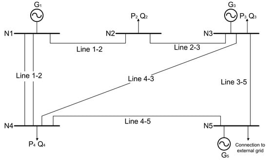
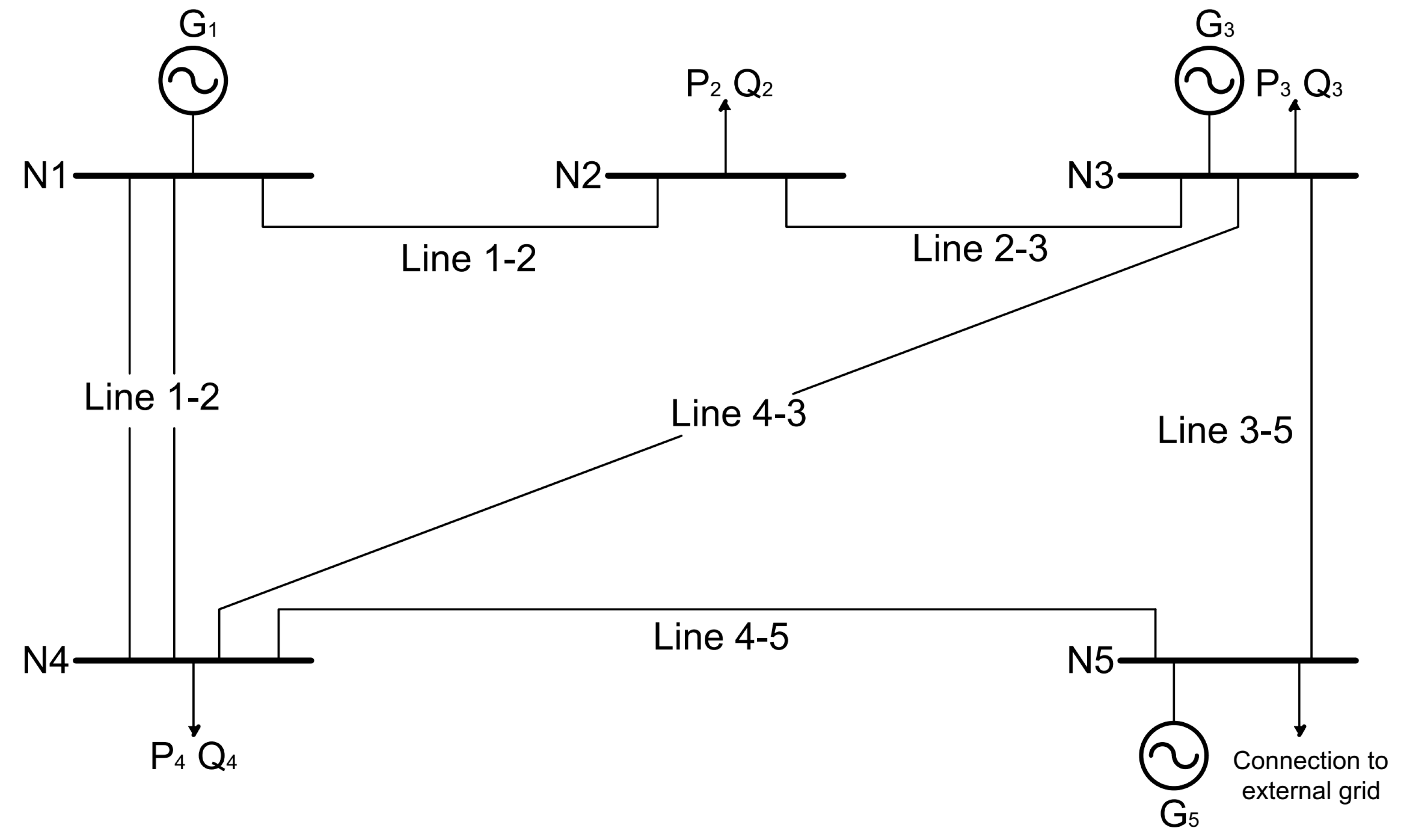
A model of a five-node segment of a closed-loop power system (Figure 1) was developed to analyze transient phenomena in high-voltage transmission networks. The study was carried out using an equivalent representation of an electric power system (EPS) operating at a nominal voltage of 400 kV. In the laboratory model, it was assumed that the parameters of the 400 V model line should correspond to those of a 400 kV transmission line. This assumption required adopting a voltage scaling ratio of η_U = 1000:1 (national transmission voltage: 400 kV → model: 400 V). However, it is not possible to complete the model using only the voltage ratio while maintaining constant power. Therefore, the estimated performance of the external power supply led to the adoption of a power-based scaling ratio of η_S = 25,000:1, meaning that each 1 kW in the laboratory model corresponds to 25 MW in the real system. This scaling relationship resulted in the following current ratio: η_I = η_S/η_U = 25,000/1000 = 25. The assumed maximum continuous current of the model line was 30 A, which corresponds to a current of 750 A in the actual transmission system. All laboratory system parameters along with their identification are provided in the publication [36]. Appropriate current and voltage transformer ratios were assumed, enabling scaling of measured signals to realistic power levels. This allowed for simulation of real-world operating conditions in high-voltage grids [37].

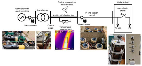
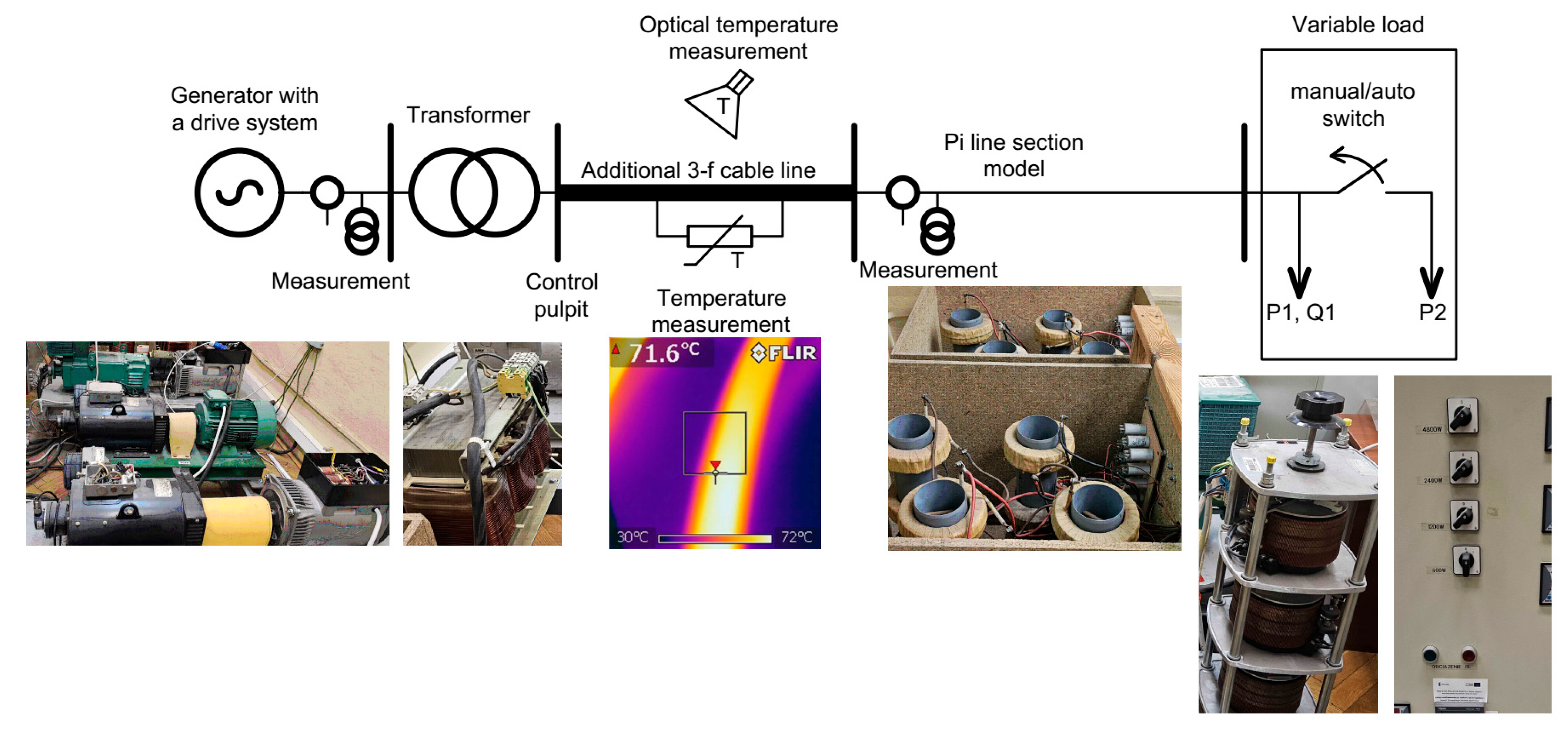
For the purpose of conducting this study, the configuration of the measurement system was modified. The actual system configuration is shown in Figure 2. The system was configured as follows. The number of generators was limited to a single unit with a rated power of 9.6 kW, driven and controlled by a drive system consisting of a DC motor regulated by a MENTOR controller (Nidec Control Techniques Ltd., Newtown, UK). The generator was set to operate in swing mode in order to respond to power variations. The excitation controller settings were adjusted in such a way that a sudden (and large relative to the generator’s rated power) step change in load power would cause a temporary voltage drop throughout the entire configured system. The phenomenon of voltage reduction in the generator due to sudden loading was superimposed on the voltage drop induced by the step change in line current, resulting in a simulated voltage sag. The generator was connected to the system via a 10.6 kW transformer with a 1:1 turns ratio. For experimental purposes, a three single-core cable (3 × N2XH 2.5 mm²) with a cross-section of 4 mm² was introduced (with length of 10 m), supplying a π-type system line consisting of five sections, each representing a 400 kV transmission line with a length of 30 km. At the end of the line, an RL-type load was connected via a contactor controlled by a relay. The inductive component of the load could be smoothly adjusted, while the resistive (active) component was applied in discrete steps. The relay controlling the contactor was operated via a Siemens LOGO controller (Siemens AG, Munich, Germany). In the setup, voltage and current measurements were carried out using LEM transducers connected to a National Instruments measurement card, both at the generator output terminals and at the bus coupling the five-section line with the load (Figure 2). Additionally, the cable connecting the transformer with the π-type line model was instrumented with thermocouples (Thermocouple Type K, Omega Engineering Inc., Norwalk, CT, USA) and monitored with a FLIR thermal imaging camera in order to record temperature variations during cyclic voltage sag events.

During normal operation, the generator was loaded with an active power of 1800 W and a reactive power corresponding to a power factor (cos φ) of 0.9 (smoothly adjusted). After the step connection of an active load, the power factor cos(φ) increases to values close to unity. The model includes laboratory simulations of voltage sags induced by sudden connection additional large-power loads—specifically, 7200 W resistive loads. Considering the applied power scaling ratio, these correspond to 180 MW load steps at the transmission level. However, in the article, the actual voltage and current values measured in the laboratory setup will be presented, without taking voltage or current transformers into account. This approach allows a clear demonstration of the efficiency of the optimization algorithm based on limiting the operating temperature of the conductor in a cable incorporated into the laboratory system for the purpose of conducting the experiment.

Before tests, the laboratory set was loaded continuously with an active power of 1800 W and a reactive power corresponding to a power factor equal of 0.93 to get the stable temperature of the additional instrumented cable. Then, through the controller, a 7200 W load was intermittently connected and disconnected in one-second intervals. Each load step was applied for 1 s, after which the additional load was disconnected (the process continued until the cable incorporated in the measurement setup reached a steady temperature, as monitored by both a thermocouple and a thermal imaging camera, as is shown in Figure 2). In the laboratory model of a fragment of the power system supplied by a single generator unit (Figure 2), the abrupt change in load leads to observable voltage dips, the depth of which depends on the magnitude of the connected load (Figure 2). This setup allowed emulation of voltage sag events associated with generator dynamic response and its control systems, such as the automatic voltage regulator (AVR) and governor.

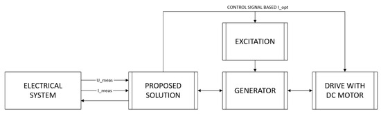
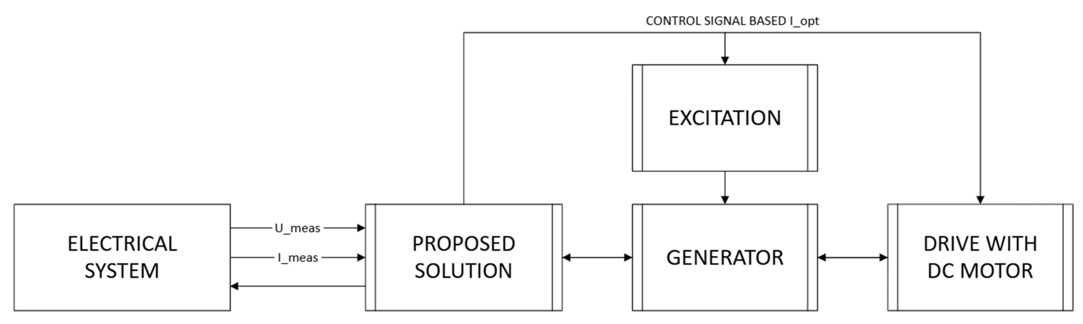
The point of integration of the optimization system, together with the control signals, is shown in the simplified block diagram in Figure 3. The proposed solution block operates on the basis of the equations provided in Section 2 and in reference [31].

The primary objective of the modeling was to introduce dynamic, non-steady-state conditions into the system, enabling the study of transient behavior and the evaluation of optimization algorithms aimed at improving power quality, minimizing energy losses, and enhancing overall stability of the transmission network under disturbance conditions.

Additionally, research is evaluated to assess the influence of an energy flow optimization algorithm—designed to reduce transient active power fluctuations—on the thermal behavior of low-voltage distribution cables during repeated voltage sags caused by load increases. The study aimed to verify whether improved control and current shaping can reduce power losses and prevent thermal overload, particularly under long-lasting disturbances. Cable thermal behavior model with a 10-m section of 3 × N2XH 2.5 mm² cable.

The currents and voltages in the line circuit were recorded using the NI 782263-01 data acquisition card (2 MS/s) (National Instruments Corporation, Austin, TX, USA), with a sampling frequency of 100 kHz per channel in high-resolution mode, which meets the requirements for the number and completeness of measurements in transient state studies. Current measurement was performed indirectly using the LEM IN 400-S sensor (LEM International SA, Meyrin, Switzerland) and voltage measurement indirectly using the LEM LV 100-500 sensor (LEM International SA, Meyrin, Switzerland)—both devices characterized by high accuracy and low temperature drift. Measurement error and uncertainty: the LEM transducers specify linearity below 0.1% and temperature deviation around ±0.05%; the NI card provides 16-bit resolution and precise channel synchronization. Temperature measurement was carried out using a FLIR E8 Pro infrared camera (FLIR Systems AB, Taby, Sweden) with a thermal sensitivity of 0.06 °C.

4. Results of Laboratory Tests

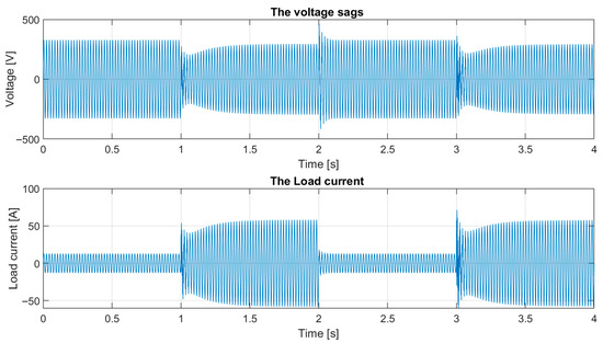
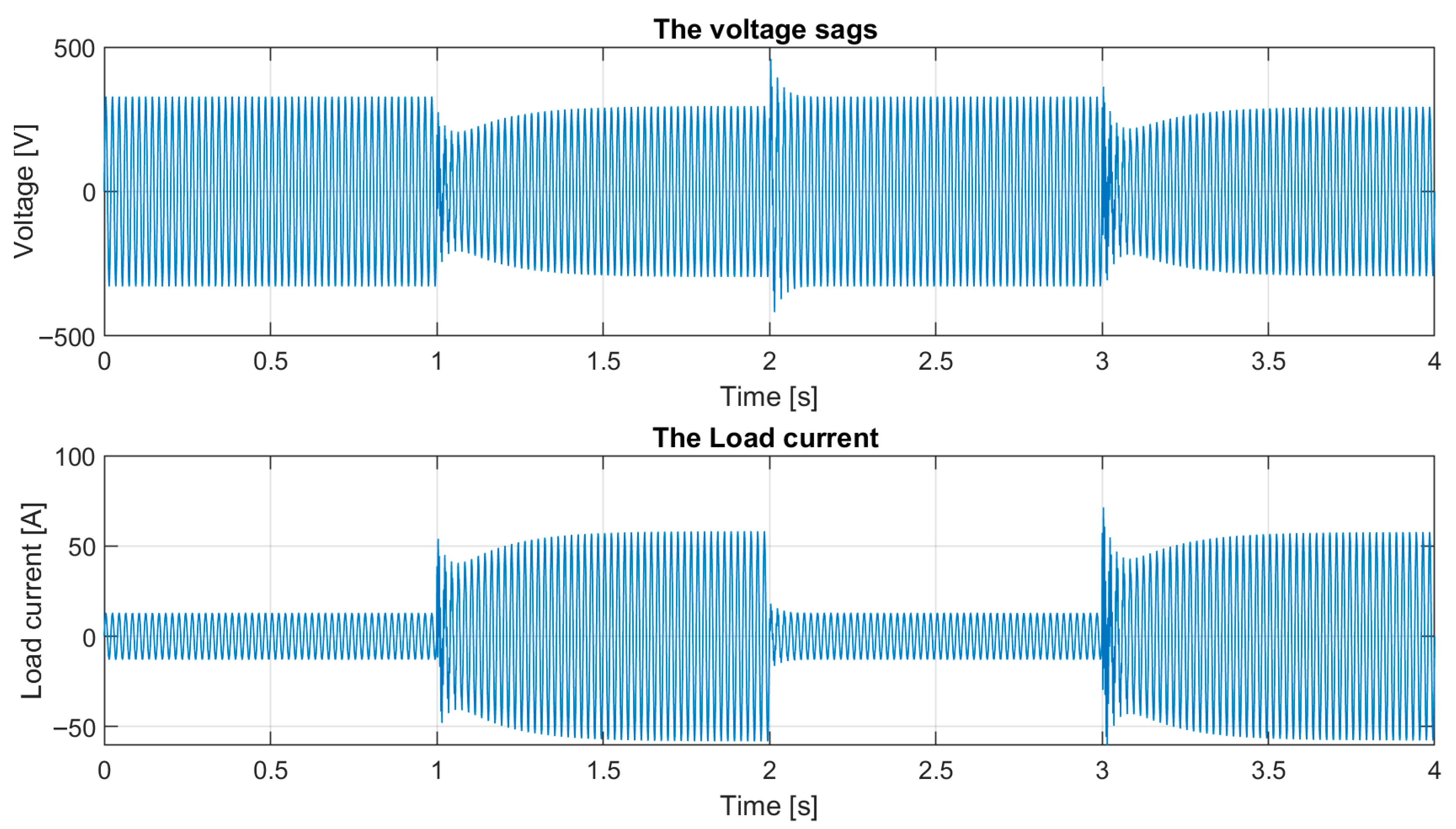
In the laboratory setup described in Section 3, during the test procedure, the voltage and current of the Pi-type line model, as well as the temperature variations in the additional cable incorporated into the measurement circuit, were recorded. The measurement results of voltage and current for two measurement periods (corresponding to two voltage sag events) are shown in Figure 4.

Voltage sag(s) (Figure 4) are associated with a sudden step increase in load current and an abrupt voltage drop, but primarily with the action of the excitation regulators and the control systems of the generator unit’s prime mover (a slow responding control system that does not adequately follow the step changes).

Table 1. Data for the reported baseline voltage sags.

Sag no.	Sag Depth [%]	Sag Duration [ms]	Recovery Ramp (Post-Sag) [s]	THD/TE Window [%]
1	13.2	1006	0.259	2.8/4.7/3.0
2	12.8	1002	0.286	2.9/5.0/3.1 *

shows the analysis of the baseline voltage sag events. It should be noted that the last value (marked with *) is related to the recovery after second sag which does not occur in presented waveforms but was added for data completeness. As one of the components in the conversion path, a MENTOR II drive converter/regulator was used. It is equipped with PID controllers for current and speed, featuring an auto-tuning option. The MENTOR II operated in four-quadrant mode. In

Table 2. MENTOR II auto-tune current loop parameters.

Parameter	Typical Range After Auto-Tune
Current loop gain	2.5–4.5
Current loop integral time	1.0–3.0 ms
Current rate limit	500–1200 A/s

, typical ranges of regulator parameter variations obtained after autotuning are presented, depending on the parameters of the driven system. During the voltage sag modeling, the proportional gain was reduced, and the integral time constant was increased (with respect to the output parameters obtained after autotuning) in order to extend the response time and accurately reproduce the voltage recovery ramp.

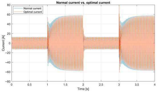
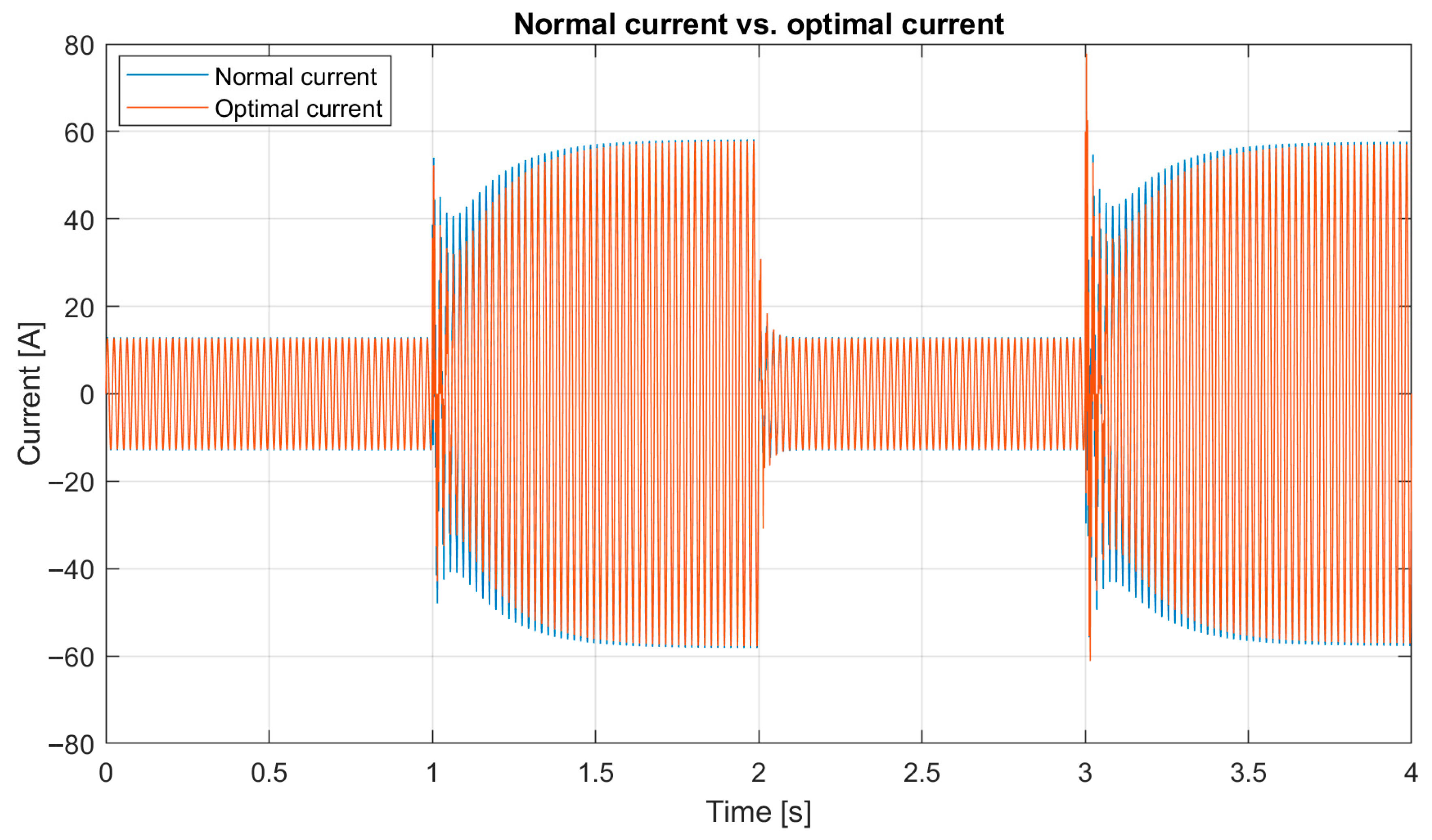
Based on the disturbed current and voltage waveforms, as well as the relationships described in Section 2 and the literature references [30,31,34], a device with a dedicated control algorithm was developed to enable optimization of the current flowing through the transmission system. The parameters of the proposed solution were optimized for a specific load variation. Future work will focus on enabling automatic adjustment of the system parameters to the characteristics of the load changes. The effect of the proposed solution is shown in Figure 5.

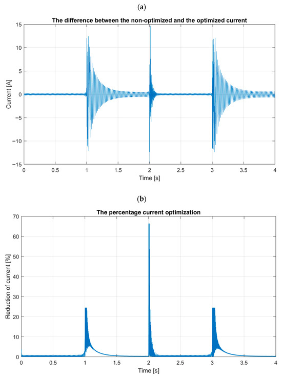
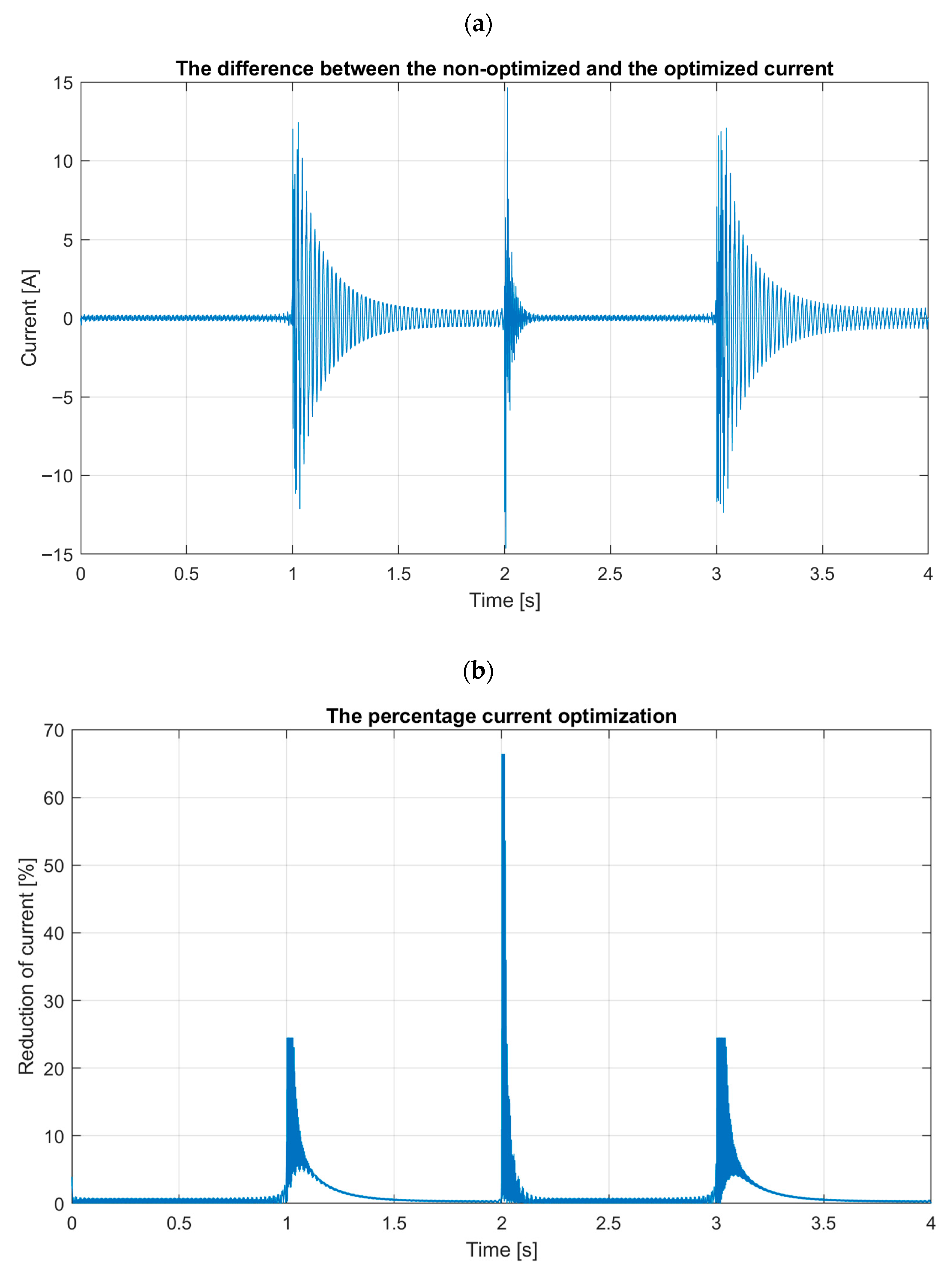
The difference between the optimized current and the current without the optimization system is shown in Figure 6. The most significant differences are observed precisely during transient states; therefore, the proposed solution can substantially contribute to the optimization of electric power flow under disturbance conditions, resulting in a reduction in loading on transmission systems, including transmission lines. This is particularly important in situations where the power network experiences frequent transient conditions, such as multiple short circuits, or in supply systems—such as isolated networks with distributed energy sources—where stability is insufficient, and load variations can cause frequent voltage fluctuations (transient states) or even relatively shallow voltage sags.

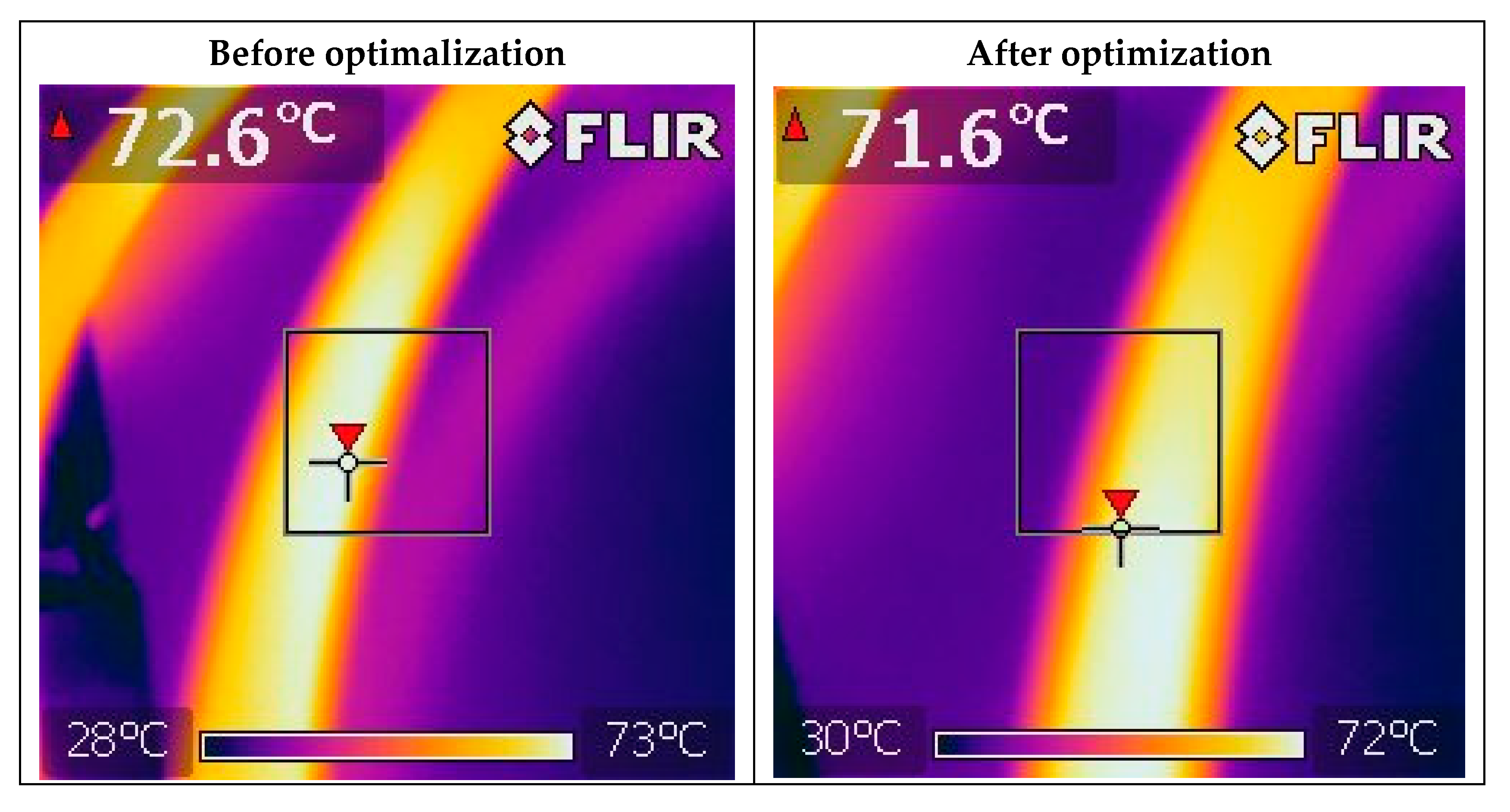
The reduction in the RMS value of the optimized current compared to the current flowing in the disturbed system before optimization, as shown in the time-domain waveform in Figure 6, leads to a decrease in the operating temperature of all components involved in the transmission and transformation of electrical energy. To demonstrate the extent to which the proposed optimization system can reduce thermal losses, a section of cable was introduced into the laboratory model of the power system and instrumented according to the description provided in Section 3. The temperature measurement results after 20 min of continuous cyclic load variations (as described in Section 3), recorded with a thermal imaging camera following the achievement of thermal steady state, are shown in Figure 7. It should be noted that the temperature stabilization after the specified time was confirmed experimentally and computationally using the finite element method.

In the measurements performed using thermocouples, the recorded temperatures were 72.69 °C before optimization and 71.48 °C after optimization. The measured temperature difference was approximately 1 °C, which confirms that the proposed solution enables a reduction in the operating temperature of the transmission system components and improves energy flow efficiency. However, it should be emphasized that although the experiment was conducted under laboratory conditions, it represents a highly idealized case. Using the simplest mathematical model/calculations based on proportionality and the permissible cable load values, a significant difference was also achieved.

Since the load variations were symmetrical, the RMS current can be calculated based on the recorded waveform over several periods of load changes. The RMS current values obtained from currents measurements for nonoptimized and optimized current waveforms are as follows:

$$I_{\mathrm{R}\mathrm{M}\mathrm{S}\_\mathrm{N}\mathrm{a}\mathrm{t}\mathrm{u}\mathrm{r}\mathrm{a}\mathrm{l}}=27.49 \mathrm{A}\mathrm{and} I_{\mathrm{R}\mathrm{M}\mathrm{S}\_\mathrm{O}\mathrm{p}\mathrm{t}\mathrm{i}\mathrm{m}\mathrm{a}\mathrm{l}}=26.38 \mathrm{A}.$$

(20)

Thus, the temperature of a cable loaded with the RMS current value can be determined from the following relationship:

$$T_{\mathrm{cable}}=T_{\mathrm{amb}}+{\left({\displaystyle \frac{I_{\mathrm{RMS}}}{I_{\mathrm{permis}}}}\right)}^2\cdot \mathsf{\Delta }{T}_{\max }$$

(21)

where $T_{\mathrm{amb}}$—ambient temperature equal to 26 °C, $I_{\mathrm{RMS}}$—current RMS value, $I_{\mathrm{permis}}$—maximum permissible continuous load current for XLPE (according to PN/IEC is equal to 32 A for 2.5 mm²), $\mathsf{\Delta }{T}_{\max }$—maximum permissible temperature rise for a given type of cable insulation (for XLPE according to PN/IEC and for $T_{\mathrm{amb}}$ is equal to 64 °C).

Based on these simple calculations, the cable temperature in the case of the non-optimized current is approximately equal to 73 °C, whereas for the optimized current it will be 70 °C. The large difference compared to the measured values results from numerous simplifications assumed in the calculations.

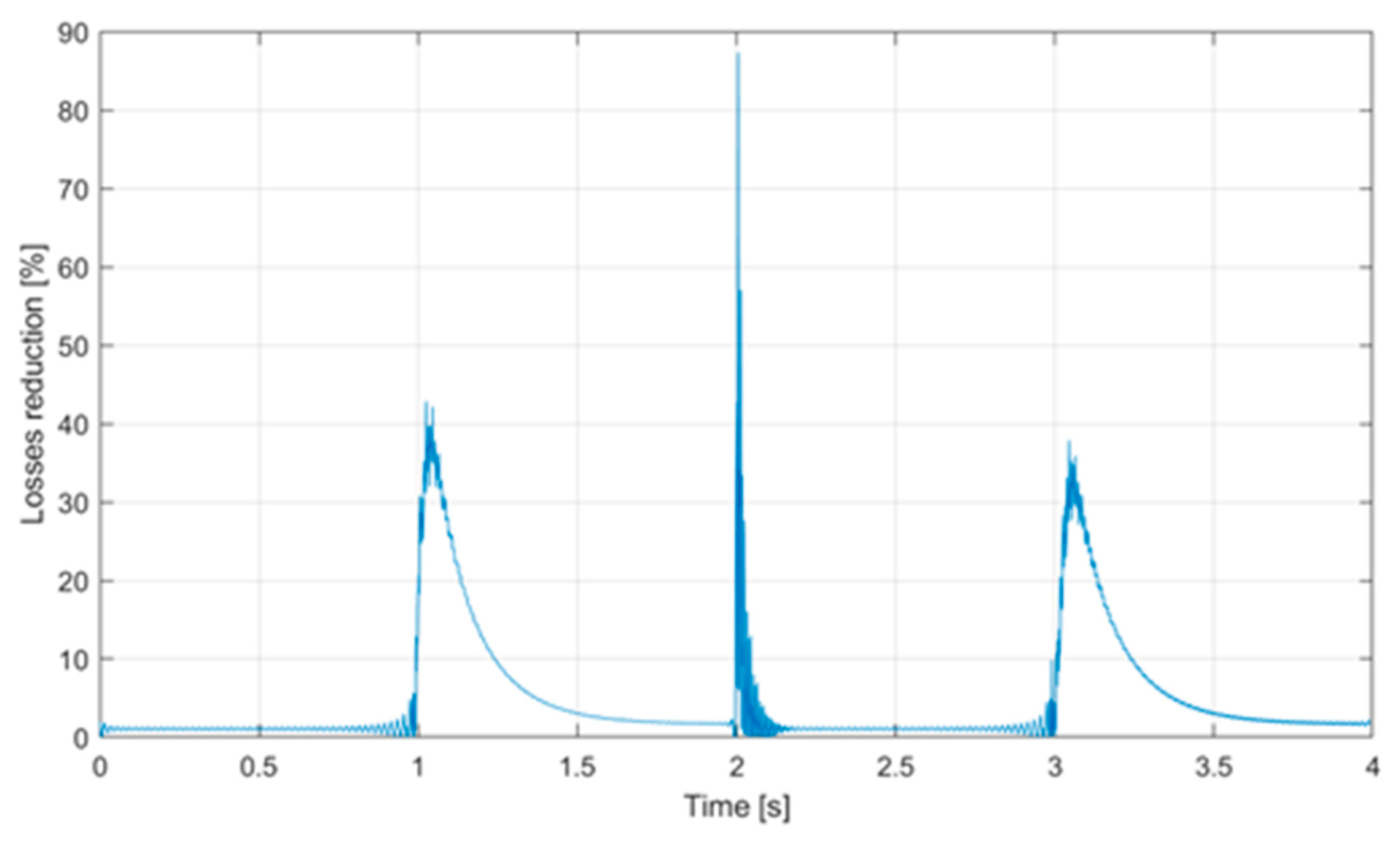
The reduction in the RMS current during transient states associated with sudden load changes, as shown in Figure 5 and Figure 6, leads to improved efficiency of electrical energy transmission, especially in unstable power supply networks, as well as to a decrease in transmission power losses. Figure 8 illustrates the nature of power loss variations introduced by current optimization.

Assuming such a continuous mode of disturbed operation of the transmission system, the reduction in power losses in per-unit terms is proportional to the square of the ratio of the two aforementioned currents (${\displaystyle \frac{{I_{\mathrm{RMS}\_\mathrm{Optimal}}}^2}{{I_{\mathrm{RMS}\_\mathrm{Natural}}}^2}}$) and amounts to approximately 7.9%. Considering the fact that the temperature rise of all transmission system components increases their resistance, the effectiveness of the method under actual operating conditions may be even higher.

From all the measurements obtained, the results proved to be mutually consistent: the maximum deviation of a single test from the mean value was +1.2%, and the minimum deviation was −0.7%. Based on these data, the standard deviation was estimated (using the “range rule of thumb” method): range of deviations = 1.2% − (−0.7%) = 1.9%; estimated standard deviation: SD ≈ range/4 ≈ 1.9%/4 = 0.475% (a conservative estimate for samples with approximately normal distribution); for n ≈ 50, the half-width of the 95% confidence interval for the mean is ≈1.96‧(SD/√n) ≈ 1.96‧(0.475%/√50) ≈ ±0.13%.

Consequently, for about 50 trials, the uncertainty of the mean estimate (95% CI) is on the order of ±0.13% relative to the measured quantities, and the intra-series variability, expressed as SD ≈ 0.48%, is low and acceptable for this type of study. In practice, this means that the observed differences (both in temperature, RMS reduction, and power loss reduction) are statistically stable and repeatable within the examined dataset.

The results were referenced to the instrumental uncertainties of the measuring devices used in the study (as stated earlier). Current and voltage transducers (LEM IN 400-S, LEM LV 100-500): declared linearity < 0.1% (typical), temperature drift ± 0.05% (typical), taking these as the main type A-B uncertainty sources, the standard uncertainty component for current/voltage measurement can be estimated at ≈0.1%. Data acquisition card (NI 782263-01, 16-bit, synchronized channels): the 16-bit resolution relative to the signal range provides very low quantization uncertainty (typically 0.01–0.05%, depending on the input range), synchronization accuracy and anti-aliasing filtering minimize sampling errors at the selected sampling frequency of 100 kHz per channel; the estimated contribution of this component to the combined uncertainty is <0.05–0.1%.

The thermal sensitivity (NETD) of 0.06 °C enables the detection of very small temperature changes; however, the absolute accuracy of the thermal camera is worse than its sensitivity (for the camera used, typically ± 1 °C or ±1%). Therefore, for changes of about 1 °C, the thermal sensitivity ensures detectability, but the absolute temperature value carries greater uncertainty. For this reason, the conclusions in the article were mainly based on temperature differences (∆T), which can be measured with greater precision than absolute values. For temperature measurement (∆T), despite the excellent thermal sensitivity (NETD = 0.06 °C), the absolute temperature uncertainty is indeed higher, and for a single measurement may reach ± 0.5–2.0 °C. However, for temperature differences ∆T, the achievable precision is higher and primarily limited by the NETD value, yielding a repeatability-based uncertainty of about 0.1–0.3 °C under the Author’s controlled experimental conditions.

For current measurement, the combined standard uncertainty component (considering LEM + DAQ + minor sources) was conservatively estimated at ≈0.12–0.2% (u), resulting in an expanded uncertainty (k = 2, ≈95% CI) of approximately ≈ 0.24–0.4%.

It should be noted that the article presents the actual recorded values of voltages, currents, and temperatures, without applying the scaling factors, because it would not have been possible to unambiguously rescale the observed thermal effect. For the current and voltage values alone, rescaling the effects to the 400 kV system level is consistent with the adopted scaling factors. The temperature index (approximately 20 min of heating) is consistent with the first-order thermal model and has been experimentally verified.

Table 3. Chosen parameters of the laboratory implementation and the measurement system.

Parameter	Value
First-order approximation criterion	$\mid {\omega }_{\max }{\tau }_i\mid \le 0.1$ ${\omega }_{\max }=2\pi f_{\max }$
Allowable	${\tau }_i\le 0.1/{\omega }_{\max }=0.1/\left(2\pi f_{\max }\right)$
Cable thermal time constant	${\tau }_{\mathrm{th}}\approx 300 \mathrm{s}$
Sampling frequency	$f_s=100 \mathrm{kHz}\Rightarrow T_s=10 \mathsf{\mu }\mathrm{s}$
Loop delay	$T_d\approx 50 \mathsf{\mu }\mathrm{s}$
Phase stability condition	${\omega }_c{T}_d\le 0.1\Rightarrow {\omega }_c\le 0.1/T_d$
Controller cutoff frequency	$f_c={\omega }_c/2\pi \le 0.1/\left(2\pi T_d\right)$
Recommended controller bandwidth	$f_c\approx 0.6\cdot \left(0.1\right)/\left(2\pi T_d\right)$
Anti-aliasing filter	$f_{AA}\approx 0.05f_s$
Measurement low-pass filter (LPF)	$f_{LP}=(2-5)f_c$
Derivative filter	$f_D=(1-2)f_c$
Design margins	Phase ≥ 45°, Gain ≥ 6 dB
Total standard current measurement uncertainty	$u_I$ ≈ 0.12–0.2%
Expanded uncertainty (k = 2)	$U_I$ ≈ 0.24–0.4%
Thermal camera sensitivity	$\mathrm{NETD}=0.06$ °C
Uncertainty of temperature difference	$\Delta T_u$ ≈ 0.1–0.3 °C
Experimental standard deviation	$SD\approx 0.48\%$
95% confidence interval for the mean (n ≈ 50)	$C{I}_{95\%}=\pm 1.96\cdot SD/\sqrt{n}=\pm 0.13\%$

shows the most important parameters of the laboratory implementation and the measurement system.

5. Conclusions

The article presents a current optimization algorithm for the current delivered by a voltage source, which was implemented in laboratory tests using a synchronous generator driven by a DC motor controlled by a MENTOR-type converter system. The proposed algorithm was implemented in a real laboratory setup representing a model fragment of a power system. The proposed solution achieves the highest effectiveness under transient conditions. To demonstrate the operation of the optimization system, transient states of the laboratory system were intentionally induced by voltage sags caused by periodically forced sudden load changes. Voltages and currents were measured before and after optimization, and the results obtained were compared.

The proposed optimization system enabled a reduction in the instantaneous current values transmitted through the power system during the most disturbed time intervals by more than 60%, which resulted in a decrease in the RMS current value over the entire measurement range by approximately 4%. This also affected the temperature of the cable included in the test setup for comparative purposes. The current waveform optimization led to a reduction in the test cable temperature by more than one degree (according to measurements performed with an independent thermal imaging camera and temperature sensors). The reduction in RMS current value led to a decrease in the operating temperature not only of the test cable but also of all components involved in the transmission of electrical energy. This resulted in reduced transmission power losses and a decrease in the transmitted energy during transient states.

According to the measurements and calculations presented in the article, the minimization of power losses reached nearly 8%. It should be noted, however, that this result referred to continuous sequences of periodically repeating transient states, and the tested device and its parameters were tuned to specific load variation profiles. It can be expected that results achieved in transmission systems with stable power sources will not be as favorable. Nevertheless, the amount of heat energy generated during fault conditions, such as short circuits occurring in power systems, can be significantly reduced, which may extend their operational lifetime. This is particularly important in the case of multiple or recurrent faults.

The paper presents examples of results for scenarios with the smallest temperature deviations (defined as the difference between the system without optimization and the system with optimization), representing a worst-case scenario. The average statistical values of temperature rise, as well as RMS and power loss reduction, are approximately 27% higher than those shown in the paper. It should be noted that the results of the temperature measurements, or more precisely, the difference in temperature between the system with optimization and the one without optimization, were used primarily as an indicator confirming the effectiveness of the optimization, rather than as an exact measure of the quality of the optimization.

It should also be emphasized that the proposed solution is primarily intended for application in islanded networks with renewable and unstable power sources, where the supply voltage stiffness is limited.

Future work will focus on optimizing the control algorithm of the proposed device to achieve automatic adaptation of operating parameters to current and voltage in real time.

References

- Perilla, A.; Papadakis, S.; Rueda Torres, J.; van der Meijden, M.; Palensky, P.; Gonzalez-Longatt, F. Transient stability performance of power systems with high share of wind generators equipped with power-angle modulation controllers or fast local voltage controllers. Energies 2020, 13, 4205. [Google Scholar] [CrossRef] [Scilit]
- Tina, G.; Maione, G.; Licciardello, S. Evaluation of technical solutions to improve transient stability in power systems with wind power generation. Energies 2022, 15, 7055. [Google Scholar] [CrossRef] [Scilit]
- Sarajcev, P.; Kunac, A.; Petrovic, G.; Despalatovic, M. Power system transient stability assessment using stacked autoencoder and voting ensemble. Energies 2021, 14, 3148. [Google Scholar] [CrossRef] [Scilit]
- Markiewicz, H.; Klajn, A. Power Quality Application Guide: Harmonics, Flicker, and Interruptions; European Copper Institute: Brussels, Belgium, 2004. [Google Scholar]
- Shepherd, W.; Zhang, L. Power Electronics and Motor Control; Cambridge University Press: Cambridge, UK, 1998. [Google Scholar]
- Dugan, R.; McGranaghan, M.; Santoso, S.; Beaty, H. Electrical Power Systems Quality, 3rd ed.; McGraw Hill: New York, NY, USA, 2012. [Google Scholar]
- Femine, A.; Gallo, D.; Giordano, D.; Landi, C.; Luiso, M.; Signorino, D. Power quality assessment in railway traction supply system. IEEE Trans. Instrum. Meas. 2020, 69, 2355–2366. [Google Scholar] [CrossRef] [Scilit]
- De Santis, M.; Silvestri, L.; Vallotto, L.; Bella, G. Environmental and power quality assessment of railway traction power substations. In Proceedings of the 2022 6th International Conference on Green Energy and Applications (ICGEA), Singapore, 4 March 2022; pp. 147–153. [Google Scholar] [CrossRef] [Scilit]
- Bollen, M.H.J.; Ribeiro, P.F. Trends in Power Quality Monitoring and Standards. IEEE Power Eng. Rev. 2003, 23, 8–15. [Google Scholar] [CrossRef] [Scilit]
- Etxeberria-Otadui, I.; Martinez, I.; El-Sayed, M.A. A Survey of Power Quality and Dynamic Performance of Electrical Networks with Distributed Generation. IEEE Trans. Ind. Electron. 2009, 56, 1401–1413. [Google Scholar]
- Jain, S. Control strategies of shunt active power filter. In Modelling and Control of Power Electronics Converter System for Power Quality Improvements; Elsevier: Amsterdam, The Netherlands, 2018; pp. 31–84. [Google Scholar] [CrossRef] [Scilit]
- Czarnecki, L.S. Orthogonal Decomposition of the Currents in a Three-Phase Nonlinear Load Circuit with a Full Definition of Power Quantities. IEEE Trans. Instrum. Meas. 2005, 54, 30–34. [Google Scholar]
- CENELEC. Voltage Characteristics of Electricity Supplied by Public Electricity Networks; Technical Report EN50160; German Institute for Standardization: Berlin, Germany, 2010. [Google Scholar]
- Szromba, A.; Mysiński, W. Voltage-source-based conductance-signal controlled shunt active power filter. In Proceedings of the 2017 European Conference on Power Electronics and Applications, Warsaw, Poland, 11–14 September 2017; pp. 1–10. [Google Scholar] [CrossRef] [Scilit]
- Szromba, A. The Unified Power Quality Conditioner control method based on the equivalent conductance signals of the compensated load. Energies 2020, 13, 6298. [Google Scholar] [CrossRef] [Scilit]
- Gao, H.; Zhang, W.; Ren, M.; Liu, X. Three-Level Active Power Filter Based on Model Predictive Control. Electronics 2022, 11, 1291. [Google Scholar] [CrossRef] [Scilit]
- Karimi, S.; Seifinejad, H.; Moradi, H.; Bagheri, H.; Hemmati, S. Constrained FCS-MPC-Based Current Controller for Voltage Source Converters: Application to Shunt Active Power Filters. IET Electr. Power Appl. 2025, 19, e70025. [Google Scholar] [CrossRef] [Scilit]
- Rasoulian, A.; Saghafi, H.; Abbasian, M.; Delshad, M. Deep learning based model predictive control of active filter inverter as interface for photovoltaic generation. IET Renew. Power Gener. 2023, 17, 3151–3162. [Google Scholar] [CrossRef] [Scilit]
- Cheepati, K.R.; Parimalasundar, E.; Suresh, K.; Rivera, M.; Rao, M.N.; Pitchai, A. Design of a novel shunt active harmonic compensator with AUV-PQ-SRF reference current extraction, OSV-MPC and SMC techniques. Sci. Rep. 2025, 15, 28773. [Google Scholar] [CrossRef] [Scilit]
- Kusters, N.; Moore, W. On the definition of reactive power under nonsinusoidal conditions. IEEE Trans. Power Appar. Syst. 1980, 3, 1845–1854. [Google Scholar] [CrossRef] [Scilit]
- Depenbrock, M. The FDB-method, a generalized applicable tool for analyzing power relations. IEEE Trans. Power Deliv. 1993, 2, 381–387. [Google Scholar] [CrossRef] [Scilit]
- Akagi, H.; Kanazawa, Y.; Nabae, A. Instantaneous reactive power compensators comprising switching devices without energy storage components. IEEE Trans. Ind. Appl. 1984, 3, 625–630. [Google Scholar] [CrossRef] [Scilit]
- Akagi, H.; Nabae, A. The p-q theory in three-phase systems under nonsinusoidal conditions. Eur. Trans. Electr. Power 1993, 1, 27–31. [Google Scholar] [CrossRef] [Scilit]
- Moradi, B.; Kargar, A.; Abazari, S. Transient stability constrained optimal power flow solution using ant colony optimization for continuous domains (ACOR). IET Gener. Transm. Distrib. 2022, 16, 3734–3747. [Google Scholar] [CrossRef] [Scilit]
- Hernández-Mayoral, E.; Madrigal-Martínez, M.; Mina-Antonio, J.D.; Iracheta-Cortez, R.; Enríquez-Santiago, J.A.; Rodríguez-Rivera, O.; Martínez-Reyes, G.; Mendoza-Santos, E. A Comprehensive Review on Power-Quality Issues, Optimization Techniques, and Control Strategies of Microgrid Based on Renewable Energy Sources. Sustainability 2023, 15, 9847. [Google Scholar] [CrossRef] [Scilit]
- Sharma, K.K.; Gupta, A.; Kaur, G.; Kumar, R.; Chohan, J.S.; Sharma, S.; Singh, J.; Khalilpoor, N.; Issakhov, A. Power quality and transient analysis for a utility-tied interfaced distributed hybrid wind-hydro controls renewable energy generation system using generic and multiband power system stabilizers. Energy Rep. 2021, 7, 5034–5044. [Google Scholar] [CrossRef] [Scilit]
- Liu, S.; Ye, B.; Hu, P.; Wan, M.; Cao, J.; Liu, Y. Transient Stability Constraints for Optimal Power Flow Considering Wind Power Uncertainty. Energies 2025, 18, 4708. [Google Scholar] [CrossRef] [Scilit]
- Kumar, P.R.; Shravani, C.; Rajitha, M.; Reddy, C.L. A Review of Emerging Techniques for Power Quality Improvement in Renewable Energy Integration. In Proceedings of the E3S Web of Conferences 616: 2nd International Conference on Renewable Energy, Green Computing and Sustainable Development (ICREGCSD), Hyderabad, India, 21–22 February 2025; pp. 1–14. [Google Scholar] [CrossRef] [Scilit]
- Verma, R.; Gawre, S.K.; Patidar, N.P. An Extensive Study on Optimization and Control Techniques for Power Quality Improvement. In Proceedings of the 2021 2nd International Conference On Electrical Power and Energy Systems (ICEPES), Bhopal, India, 10–11 December 2021; p. 9699504. [Google Scholar] [CrossRef] [Scilit]
- Hawron, K.; Rozegnał, B.; Sułowicz, M. Transient Active Power in Two-Terminal Networks. Energies 2024, 17, 4620. [Google Scholar] [CrossRef] [Scilit]
- Hawron, K.; Rozegnał, B.; Sułowicz, M. Optimum Energy Flow from Source in Transient State. Energies 2025, 18, 281. [Google Scholar] [CrossRef] [Scilit]
- Saribulut, L.; Ameen, A. Voltage Sag Detection and Compensation Signal Extraction for Power Quality Mitigation Devices. Energies 2023, 16, 5999. [Google Scholar] [CrossRef] [Scilit]
- Erazo-Caicedo, D.; Mojica-Nava, E.; Revelo-Fuelagán, J. Model predictive control for optimal power flow in grid-connected unbalanced microgrids. Electr. Power Syst. Res. 2022, 209, 108000. [Google Scholar] [CrossRef] [Scilit]
- Siwczyński, M.; Hawron, K. Distribution of G and B parameters of two-port electrical networks and their modulation disturbances. Electr. Rev. 2015, 91, 257–261. [Google Scholar] [CrossRef] [Scilit]
- Siwczyński, M.; Hawron, K. Optimum tasks and solutions for energy transmission from the source to the receiver. Bull. Pol. Acad. Sci. Tech. Sci. 2018, 66, 655–663. [Google Scholar] [CrossRef] [Scilit]
- Szczepanik, J.; Rozegnał, B. The Development of the Real Life Model of the Five Node Power System. Czas. Techn. 2015, 2-E, 83–102. [Google Scholar] [CrossRef]
- Szczepanik, J.; Rozegnał, B. Laboratory Power System Model Designed for Testing Dynamic Processes. Acta Energ. 2016, 2, 195–208. [Google Scholar] [CrossRef] [Scilit]
Disclaimer/Publisher’s Note: The statements, opinions and data contained in all publications are solely those of the individual author(s) and contributor(s) and not of MDPI and/or the editor(s). MDPI and/or the editor(s) disclaim responsibility for any injury to people or property resulting from any ideas, methods, instructions or products referred to in the content. |
© 2025 by the authors. Licensee MDPI, Basel, Switzerland. This article is an open access article distributed under the terms and conditions of the Creative Commons Attribution (CC BY) license (https://creativecommons.org/licenses/by/4.0/).