Abstract
Climate change and rising temperatures in cities due to the urban heat island (UHI) effect are causing increased heat stress and driving the development of efficient, sustainable outdoor cooling systems. The aim of this article was to analyze the integration of adiabatic air cooling systems with photovoltaic (PV) installations in the context of improving thermal comfort and energy autonomy. The study was conducted on the example of a bus station in Rzeszow (Poland), considering two system variants: indirect evaporative cooling and direct evaporative cooling. To assess the impact of comfort parameters on the number of hours of system operation, energy consumption, and operating costs, four upper thermal comfort limits were considered: 22 °C, 22.9 °C, 24 °C, and 25 °C. The results indicate that increasing the upper limit of thermal comfort reduces the operating time of the system and significantly reduces the demand for cooling—for example, increasing the thermal comfort range from 22.9 °C to 24 °C reduces useful energy by 41%. Assuming a thermal comfort range of 25 °C, the direct evaporative cooling system achieves full energy autonomy and is fully powered by photovoltaics. Life cycle analysis (LCA) and life cycle cost (LCC) confirmed the environmental and economic benefits of using higher thermal comfort values. The study highlights the potential of adiabatic cooling systems, in conjunction with a local photovoltaic installation, as an adaptive solution that improves thermal comfort in urban spaces with minimal energy consumption from the grid.
1. Introduction
Urban heat islands (UHIs) and the increasing frequency of heat waves pose a growing challenge to public health and quality of life, especially in areas with high building density and limited vegetation [1,2,3]. The literature emphasizes the growing importance of thermal comfort in outdoor spaces, which affects mobility, social activity, and the attractiveness of public spaces [4,5,6,7,8,9]. As a result, there is a growing demand for solutions to improve the microclimate in open urban areas, such as squares, platforms, and transport hubs [10].
In response to these needs, both passive cooling strategies, such as shading, urban greenery, and the use of high-albedo materials [11,12,13,14,15,16], and active technical systems [17,18,19,20,21,22,23,24] are being developed. One of the most promising technologies is adiabatic cooling systems, which are characterized by low energy consumption and the absence of synthetic refrigerants [22,23,24,25]. However, the efficiency of both direct (DEC) and indirect (IEC) adiabatic cooling depends on humidity conditions, water quality, and the characteristics of the usable space [26,27,28,29,30,31,32,33,34,35,36,37,38,39].
An important direction of development is the integration of adiabatic systems with photovoltaic (PV) installations. The demand for cooling in outdoor spaces coincides with the maximum energy production from PV, which increases the energy autonomy of the system and reduces operating costs [40,41]. In addition, lowering the temperature of PV modules during operation can improve their efficiency, which is an additional benefit of integration [42,43,44,45].
However, there is still a lack of analysis in the literature on the application of such solutions in open transport spaces, which are characterized by highly variable environmental conditions and a large number of users. There is also a lack of studies that take into account long-term meteorological data and assess the impact of various thermal comfort criteria on cooling load, energy autonomy, economic indicators, and environmental impact.
The aim of this article is to expand the existing knowledge on adiabatic air cooling systems in outdoor areas, using the example of a local railway station in Rzeszów (Poland) [25]. The analysis includes proposing alternative variants of air cooling endpoints, the selection of which allows for the identification of different cooling power demand values. Changes in the cooling load can significantly affect the energy balance of the system, operating costs, and environmental footprint. An important aspect of the study is also the assessment of the synergy between the cooling system and the existing photovoltaic installation, which allows for consideration of integration within the concept of hybrid systems.
The final result of the analysis is to identify a cooling endpoint that ensures a high level of energy autonomy for the system under study, in line with the principles of sustainable development and optimization of building infrastructure operation. Thanks to this approach, the work fills a gap in the literature by providing a comprehensive assessment of adiabatic cooling systems based on long-term meteorological data and actual energy yields from PV installations, which highlights the innovative nature of the proposed approach.
2. Object of Research
2.1. Characteristics of the Test Object
The analyzed object is a bus station platform in Rzeszow (Poland), which is an open, semi-covered usable space intended for passengers (Figure 1). The roof structure is made of photovoltaic modules, which allows for the integration of a cooling system with a local renewable energy source. The key operational and geometric parameters are presented in Table 1.
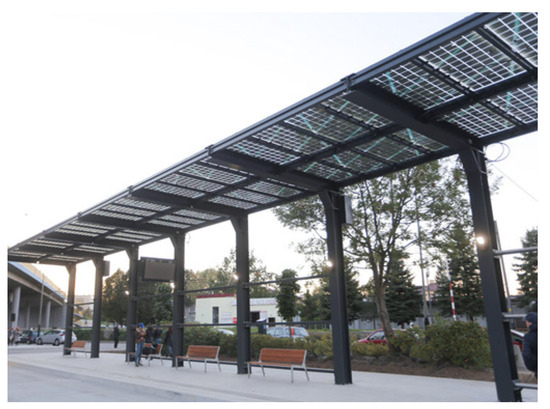
Figure 1.
The object of the study—the platform of a local railway station in Rzeszów (Poland).

Table 1.
Basic data of the test object [25].
2.2. Selection and Description of Cooling System Variants
This paper analyzes two variants of adiabatic cooling, which, according to a previous multi-criteria assessment [25], are characterized by the highest energy and economic efficiency and the lowest environmental impact. Both systems were integrated with the existing photovoltaic installation, which is a local source of electricity:
(a) PKW/PV-CP-KW variant—indirect evaporative cooling (P—indirect, KW—evaporative air conditioning, PV—power supply with PV modules, CP—cool air, KW—air supply grille).
In this solution, the air is cooled in a central evaporative device without changing its moisture content and then fed into the usable area through ventilation ducts and supply grilles (Figure 2). This variant increases user comfort without affecting air humidity.
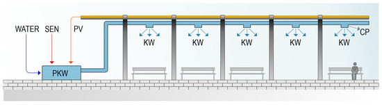
Figure 2.
Diagram of the air cooling system in the PKW/PV-CP-KW variant [25].
(b) BKW/PV-CP-KW variant—direct evaporative cooling (B—direct, KW—evaporative air conditioning, PV—PV module power supply, CP—cool air, KW—air supply grille).
In this system, the air is cooled and humidified directly in the air conditioning unit and then directed through a short duct to the occupied space (Figure 3). This solution is characterized by higher cooling efficiency at high air temperatures.
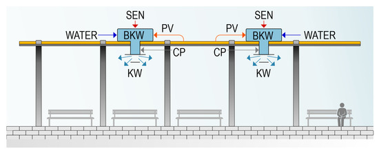
Figure 3.
Diagram of the air cooling system in the BKW/PV-CP-KW variant [25].
In both variants, water is the primary working medium, while electricity from the PV system and power grid (SEN) is used to power fans and circulation pumps. Table 2 summarizes the technical parameters of the selected devices.
Table 2.
Technical parameters of the devices adopted in the analyzed variants of the cooling system.
3. Research Methodology
3.1. Determination of Thermal Comfort Parameters
The analysis used meteorological data on outdoor air parameters from the Rzeszow–Jasionka meteorological station in Poland, which is located at the geographical coordinates 50°06′ N, 22°03′ E. These data, made available by the Institute of Meteorology and Water Management in Warsaw [46], include daily and hourly series covering key atmospheric parameters, such as air temperature, relative humidity and wind speed. These parameters were recorded between 2012 and 2019.
Thermal comfort assessment indicators are used to evaluate the thermal load on the human body. Over the past few decades, a number of indicators based on human heat balance have been developed. These differ in terms of the complexity of the calculations, the input data requirements, and the degree to which they are suited to external conditions. The following indicators are most often used in field research and numerical simulations [47,48,49,50,51]:
- PET (Physiological Equivalent Temperature);
- UTCI (Universal Thermal Climate Index);
- WBGT (Wet-Bulb Globe Temperature);
- SET (Standard Effective Temperature).
Against the background of the above indicators, the effective temperature (TE) according to Missenard could play a significant role in field studies [25]. Its main advantages are the simplicity of the calculations and the limited input requirements. As it does not require complex data on solar radiation or anthropometric parameters to be taken into account, this indicator is easy to use in field research, especially where the availability of measurement equipment is limited.
Taking the above arguments into account, the range of thermal comfort outdoors for the purposes of this analysis was determined using the effective temperature index (TE). This index is calculated based on Missenard’s formula [25] and depends on air temperature (T), wind speed (w) and relative humidity (RH):
- For w < of 0.3 m/s:
- For w ≥ of 0.3 m/s:
The TE index values were calculated for each hour between 1 June and 31 August from 2012 to 2019, based on real meteorological data [46]. The analysis was limited to the summer months (June, July and August), which are characterized by the highest air temperatures. Temperature and relative humidity data were obtained from the Rzeszow–Jasionka meteorological station.
Relative air humidity was taken into account in accordance with actual meteorological data, influencing the determination of thermal comfort indicators. However, the impact of humidity on the efficiency of adiabatic cooling was not analyzed in this study. This issue has been identified as a direction for future research on system optimization.
The analysis assumed airflow levels within the human impact layer. Actual wind speed values obtained from meteorological data were converted to a height of 1 m above ground level. This took into account the roughness of the ground and made it possible to recreate the sensation of air movement in the usable space. A detailed description of the conversion process is provided below [52,53]:
Symbols: —wind velocity at height Z, —wind velocity at wind meter height, —height under study Z, —height of wind meter measurement, —aerodynamic roughness coefficient.
The reference area was defined as the space occupied by people within three bus parking spaces, at a height of 2 m. In this area, the wind speed was halved at a height of 1 m above ground level. The aerodynamic roughness coefficient was assumed to have a value of 2 (Z0 = 2), corresponding to urban areas with a medium development intensity in cities with a population of between 100 and 500 thousand inhabitants [53].
The level of thermal comfort was determined on the basis of the calculated values of the effective temperature index TE (according to dependencies (1) and (2)). The Mikhailov scale (Table 3) was used for classification, distinguishing between categories of human thermal sensation [48]. According to the Mikhailov scale, comfort conditions are in the TE value range of 21–22.9 °C.
Table 3.
Mikhailov Scale [48].
This analysis uses a multivariate approach to determine the upper limit of thermal comfort. This allows for a more comprehensive assessment of the impact of weather conditions on cooling demand. As part of the study, four variants of the upper comfort limit were adopted: TEmax = 22 °C, TEmax = 22.9 °C, TEmax = 24 °C, and TEmax = 25 °C. This approach enables the sensitivity of cooling systems to the adopted comfort criteria to be analyzed and the hours when it is necessary to start up the refrigeration system to be identified.
Taking into account the various upper comfort limits enables us to determine the point at which the cooling capacity can be generated with the support of the existing photovoltaic system, thereby ensuring the system’s energy autonomy. This approach enables the technical parameters of the cooling system to be optimized, ensuring user comfort with minimal energy consumption from the power grid.
3.2. Calculation of Cooling Capacity
The cooling capacity demand was calculated on the assumption that the cold supplied to the analyzed QCH zone should completely balance the total QZC heat gains generated in the outdoor zone. QZC total heat gain consists of two components:
- Variable gains (QZC-Z)—calculated on the basis of instantaneous parameters of the outside air;
- Fixed profits (QZC−S)—resulting from heat emission by sources present in the examined facility.
The relationship between these quantities is expressed by the equation [25]:
The variable heat gains, resulting from the amount of heat received by the flowing air stream (QZC−Z), were calculated based on the instantaneous parameters of the outside air, using the relationship:
Symbols: —mass flow rate, —difference in specific enthalpy of air, —enthalpy of supply air, —air enthalpy in the reference zone.
The supply air mass flux was calculated on the basis of the formula:
Symbols: —volume flow rate, —air density.
The volume flow of supply air was calculated on the basis of:
Symbols: F—horizontal airflow area (assuming F = 72 m2).
The starting point of the cooling process (P1) was determined based on the actual parameters of the outdoor air recorded during the hours when cooling was required. The endpoint of the cooling process (P2) is defined by the air parameters described by T2. The T2 value was calculated by converting dependency (2) into the TE indicator using the following formula:
This analysis is based on the assumption that the value of the T2 parameter can be one of four different values: 22 °C, 22.9 °C, 24 °C or 25 °C. The rationale behind this selection is that 22 °C corresponds to the “middle” of the thermal comfort range on the Mikhailov scale [48], whereas 22.9 °C marks the upper limit of thermal comfort on the same scale. The values of 24 °C and 25 °C fall outside the thermal comfort range but were considered to determine the point at which the cooling system can operate autonomously using the power generated by the existing PV system.
As the analyzed space refers to a covered area, direct solar radiation was omitted from the heat balance. However, heat emitted by users and the environment was included as constant heat gains (QZC-S). Measurements of the actual average radiation temperature in situ were incorporated into the planned research. The constant heat gains observed in the study area are due to people staying in the zone and motor vehicles located in its immediate vicinity. The paper [25] presents a detailed methodology for determining this type of heat gain. The results of the constant heat gain calculations are taken from this publication, and a summary of the values is presented in Table 4.
Table 4.
Results of calculations of constant heat gains QZC-S, for the research object [25].
3.3. Determination of Solar Radiation Potential
To determine the solar radiation potential of the facility under study, an analysis was carried out of the actual electricity yields from the existing photovoltaic installation acting as a roof over the external cooling zone. Energy generation by the PV installation was measured through the Energy Management System, which enabled remote monitoring of the system’s operation.
For the analysis, the daily electricity yields from June, July and August 2019 were taken into account. Only the days on which cooling was required were selected for the analysis; these were the days on which the effective temperature index exceeded the set limit values for the individual comfort variants (22 °C, 22.9 °C, 24 °C and 25 °C).
3.4. Comparative Analysis of the Assumed Variants
3.4.1. Energy Effect
The energy effect of the individual cooling variants was calculated based on the demand for primary (), final () and useful energy (), in accordance with the guidelines set out in paper [54]. The following formulas were used for this purpose:
- Annual primary energy demand, EP:
- Annual final energy demand, EK:
- Annual usable energy demand, EU:
The annual primary energy demand, denoted (Qp), signifies the annual non-renewable primary energy demand for the cooling system, defined as (Qp,C).
Symbols: —generation and delivery of the energy carrier or energy for the cooling system, —annual support final energy demand for cooling system, —for the generation and supply of electricity, specifically for the annual auxiliary energy demand of the cooling system.
To determine the annual final energy demand () for the cooling system (), the following relationship was assumed:
Symbols: —seasonal average total efficiency of cooling system, —average seasonal coefficient of energy efficiency of cooling production, —seasonal average cooling storage efficiency, —seasonal average efficiency of cooling distribution from cooling source to cooled area, —average seasonal efficiency of control and usage of cooling in cooled area, —reference average coefficient of energy efficiency of cold production, —correction factor depending on cooling system.
The values of the coefficients employed in the calculation of the energy effect, contingent on the variant of the installation, are presented in Table 5.
Table 5.
Comparison of the coefficients adopted for the calculation of the energy effect [54].
3.4.2. Environmental Effect (LCA)
The proposed variants of the air cooling system in the outdoor zone were assessed in terms of environmental impact using life cycle analysis (LCA) in accordance with the standards [55,56]. The Eco-indicator method was utilized for the assessment, delineating three categories of damage [57,58]: human health, ecosystem quality and natural resources. The environmental impact was calculated on the assumption of an egalitarian cultural version and a long-term perspective of technological development. The Eco-indicator values were calculated for each damage category and each installation variant, with the functional unit defined as the demand for non-renewable primary energy and a lifetime of 25 years. The present analysis is limited to the operation phase; the production and decommissioning of the equipment are not included. The calculations were based on the unit coefficients of the Eco-indicator, referring to GJ of useful energy. The values of the assumed coefficients are presented in Table 6.
Table 6.
The coefficients used in the calculation of the Eco-indicators of the impact category and the category of damage.
3.4.3. Economic Impact (LCC)
The Life Cycle Cost (LCC) method was utilized in order to conduct an economic analysis of selected variants of the cooling installation of the research facility [59,60]. This method encompasses all costs incurred throughout the product life cycle, thereby enabling the comparison of alternative design options and the selection of the optimal solution in terms of total investment and operating costs. The economic analysis in terms of LCC was conducted in this paper using the complex method, according to the formula [59,60]:
The LCC method is predicated on the analysis of discounted cash flows and incorporates various cost elements, including the consumption of useful energy carriers, maintenance and operation of the installation, as well as price volatility over the lifetime. Therefore, for each of the analyzed variants of the cooling installation, the following were determined: investment costs (), ownership costs (including, inter alia, technical inspections, servicing, cleaning, and potential repair costs, as well as operating costs related to the consumption of electricity and water from the water supply network) (), the forecasted increase in the prices of carriers (), degradation of PV cells () and the lifetime of the investment ().
3.5. Procedure for Conducting Simulations
To perform the simulation calculations, a simple spreadsheet model was developed, enabling the analysis of hourly variations in outdoor air parameters and the evaluation of thermal comfort indices. The computational model was based on meteorological data, including air temperature, relative humidity, and wind speed. The simulations were carried out according to the methodology described in Section 3.1 and Section 3.2, maintaining consistency in the assumptions related to the upper thermal comfort limits (TEmax) and the parameters of heat gains and losses in the analyzed cooling systems.
The simulation procedure included the following steps:
- Input of meteorological data into the spreadsheet;
- Calculation of the TE index on an hourly basis;
- Identification of hourly exceedances of the TE index for each of the four TEmax variants;
- Determination of cooling demand depending on the exceedance of the comfort limit,
- Calculation of useful, final, and primary energy for two cooling system variants: indirect and direct evaporative cooling;
- Comparison of the actual electricity yield from the local PV installation with the energy demand of the analyzed cooling systems;
- Calculation of the environmental impact index for each cooling system variant.
The obtained results enabled the assessment of the energy and economic performance of the analyzed cooling systems under varying climatic conditions and constitute a reference point for further analyses and model validation.
3.6. Validation and Limitations
This study used simulation calculations of heat balance and energy consumption based on actual meteorological data and electricity yields from a local photovoltaic installation in 2019. Taking measurement data from an operational PV installation into account enabled the degree to which cooling systems’ energy needs are covered, and their autonomy, to be realistically determined.
However, the limitations of the TE (effective temperature) index used should be emphasized. Like other simple temperature and humidity indices, this index does not fully take into account the influence of infrared radiation emitted by surfaces such as asphalt or variations in air flow velocity. Consequently, assessing thermal comfort using TE in an outdoor environment may result in underestimation or an inaccurate reflection of the conditions experienced by users.
Due to these limitations, in situ studies are necessary in order to apply a more reliable index: the Universal Thermal Climate Index (UTCI). The UTCI takes into account the effects of radiation, air velocity and humidity, allowing for a more realistic assessment of thermal comfort in outdoor environments.
It should also be noted that the life cycle assessment (LCA) in this study only refers to the operation stage of cooling systems. Future studies should extend the analysis to include aspects related to the production and disposal of equipment to allow a more complete assessment of the environmental impact of the entire system throughout its life cycle.
4. Results
4.1. Thermal Comfort Parameters—Range
The following Figure 4 illustrates the frequency of situations in which the value of the TE indicator exceeded the thermal comfort range under different assumptions of the upper limit of TE (TEmax). It does so by showing the number of such hourly events that occurred between 2012 and 2019.
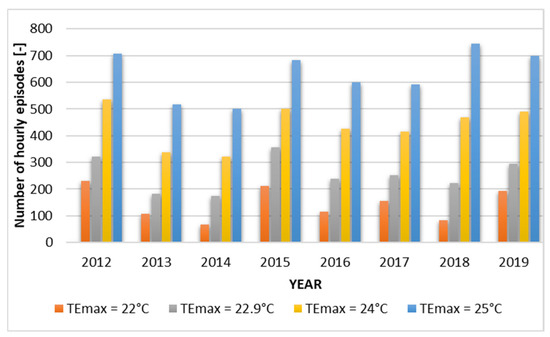
Figure 4.
The frequency of episodes when the TE index exceeded the upper limit of thermal comfort in individual years [46].
In the outdoor area under consideration, the requirement for cooling is experienced during the summer months, specifically the period spanning from June to August. In the period under analysis (2012–2019), the number of hours per season in which cooling was required, assuming the upper limit of thermal comfort according to the Mikhailov scale (TEmax = 22.9 °C), ranged from 332 to 537. This range generally corresponds to several hours per day. However, it should be emphasized that, in the coming years, the number of such events may increase significantly due to climate change, which further confirms the need to develop air cooling systems in external areas of human habitation.
Furthermore, a substantial discrepancy exists in the requisite duration for cooling, contingent on the established thermal comfort parameters. To illustrate this point, consider the effect of reducing the upper limit of the comfort index from TEmax = 22.9 °C to TEmax = 22 °C. This results in an increase in the number of cooling hours from 36% in 2014 to as much as 59% in 2018. It is evident that this will result in a substantial augmentation of the cooling system’s operational longevity. Consequently, there will be an escalation in the associated operating expenses. The augmentation of the limit to TEmax = 24 °C has been demonstrated to result in a reduction in the duration of cooling episodes, with a decline observed from 41% in 2014 to 109% in 2018. Consequently, there has been a substantial decrease in the operational duration of the cooling system, which has resulted in a minor decline in thermal comfort for human subjects.
4.2. Cooling Capacity Demand
The determination of variable heat gains QZC-Z was made on the basis of meteorological data for the area of the research facility and assuming different values of thermal comfort temperature. The calculations were executed in accordance with the methodology delineated in point 3.2 of this document. The total demand for cooling capacity necessary to ensure thermal comfort in the analyzed outdoor zone is the sum of the variable heat gains QZC−Z and the constant heat gains QZC−S, determined on the basis of the heat balance and equal to 94 kW. A comprehensive analysis was conducted to ascertain the energy requirements for cooling in each variant, with the operational hours of the air cooling system being a pivotal factor in this analysis. The results of the calculation are displayed in Figure 5.
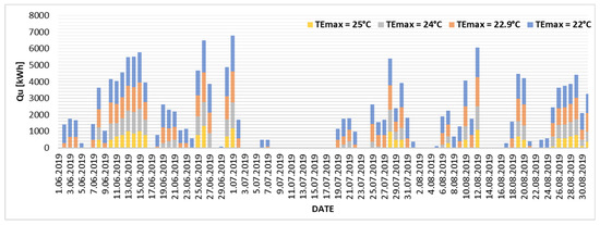
Figure 5.
The usable energy required to generate cooling by the cooling system for the individual variants.
A thorough analysis of the usable energy was conducted for the individual variants, indicating that increasing the upper limit of thermal comfort from TEmax = 22.9 °C to TEmax = 24 °C leads to a significant decline in seasonal usable energy demand, with a reduction of 41% observed (from 48,411 kWh to 28,803 kWh). Conversely, a reduction in the thermal comfort limit by 0.9 °C (up to TEmax = 22 °C) results in a 42% increase in usable energy, reaching 68,594 kWh.
4.3. Degree of Coverage of Energy Needs from PV Installations
The degree of energy demand coverage by the cooling system in relation to the different variants of the upper limit of thermal comfort (cooling endpoint) is presented, based on the actual daily electricity yields from the existing PV installation in 2019. The results are presented in Figure 6, Figure 7, Figure 8 and Figure 9. The graphs illustrate the discrepancy between the electricity produced by the PV installation (exceeding the required threshold, indicated by positive values) and the electricity that would need to be imported from the power grid (indicated by negative values). The analysis was conducted on two specific adiabatic air cooling systems: the direct evaporative cooling system (BKW/PV-CP-KW) and the indirect evaporative cooling system (PKW/PV-CP-KW).
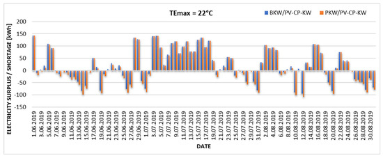
Figure 6.
Excess and daily shortage of electricity produced from the existing PV installation in the case of the upper limit of thermal comfort TEmax = 22 °C.
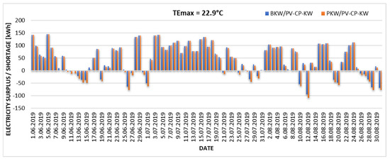
Figure 7.
Excess and daily shortage of electricity produced from the existing PV installation in the case of the upper limit of thermal comfort TEmax = 22.9 °C.
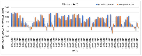
Figure 8.
Excess and daily shortage of electricity produced from the existing PV installation in the case of the upper limit of thermal comfort TEmax = 24 °C.
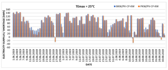
Figure 9.
Excess and daily shortage of electricity produced from the existing PV installation in the case of the upper limit of thermal comfort TEmax = 25 °C.
The graphs (Figure 6, Figure 7, Figure 8 and Figure 9) show changes in the proportion of electricity demand for cooling purposes produced by a local PV installation. With an assumed upper limit of thermal comfort of TEmax = 22 °C, the existing photovoltaic installation can cover 81% of energy needs for the BKW/PV-CP-KW installation and 77% for the PKW/PV-CP-KW system. Increasing the upper limit of thermal comfort towards higher TEmax values significantly increases the degree of coverage of energy needs for cooling. According to the Mikhailov scale (TEmax = 22.9 °C), the coverage is 87% for the BKW/PV-CP-KW installation and 83% for the PKW/PV-CP-KW system. Increasing TEmax by 1.1 °C results in 98% coverage of the electricity demand from PV for the BKW/PV-CP-KW installation and 91% for the PKW/PV-CP-KW system. The existing PV installation is only able to cover 100% of the electricity demand for the direct evaporative cooling variant (BKW/PV-CP-KW) and 97% for indirect evaporative cooling (PKW.PV-CP-KW) when the upper limit of thermal comfort is shifted to TEmax = 25 °C. This value can be considered the autonomy limit of the analyzed cooling system.
4.4. Energy Effect—Results
Based on an analysis of selected air cooling system variants in the outdoor zone and different upper limits of thermal comfort, the seasonal demand for final (EK) and primary (EP) energy was calculated, taking into account the energy effect. The EK and EP values are shown in Figure 10.
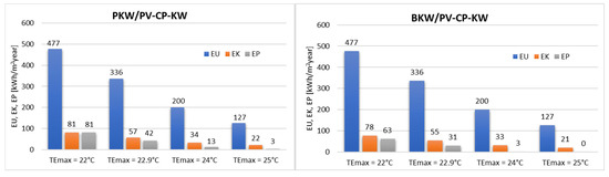
Figure 10.
The value of the EP, EK and EU indicators for the individual variants and the different assumptions of the upper limit of thermal comfort of TEmax.
The EU usable energy index is the same for both proposed cooling systems because it depends on the upper limit of the cooling range, i.e., the TEmax indicator. The lowest final, usable and primary energy requirements were recorded for the variants with the highest upper thermal comfort limit, i.e., TEmax = 25 °C. This is evident for both analyzed cooling systems. At this limit, the direct evaporative cooling system (BKW/PV-CP-KW) achieves an EP value of 0, meaning there is no use of primary energy from renewable sources. Regarding the individual thermal comfort limits, reducing the TEmax value from 22.9 °C to 22 °C increases the EP index value by 91% for the BKW/PV-CP-KW system and by 106% for the PKW/PV-CP-KW system. Changing the TEmax target value to TEmax = 24 °C results in a 41% decrease in EU and EK for both cooling system variants, while EP decreases by 68% for BKW/PV-CP-KW and by 91% for PKW/PV-CP-KW. A similar downward trend is observed in the final energy index (EK), which depends on the efficiency of the selected system, for both systems with an increase in the value of the upper limit of thermal comfort (TEmax).
4.5. Environmental Effect—LCA—Results
The Eco-indicator values were calculated for the adopted variants of air cooling system installation in the outdoor zone and for different thermal comfort limits in relation to individual environmental impact categories, which were then grouped into corresponding damage categories. Figure 11 shows the impact category indicator values for the individual installation variants, which significantly impact the final Eco-indicator value.
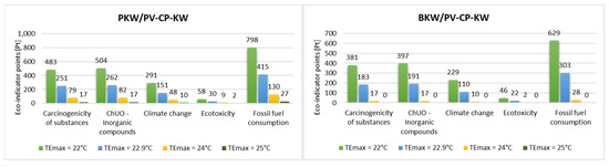
Figure 11.
Comparison of Eco-indicators of individual impact categories for the analyzed variants.
The total value of the Eco-indicator for the analyzed cooling installation variants is significantly impacted by the consumption of fossil fuels and the emission of inorganic compounds and carcinogens, as well as climate change and ecotoxicity. Studies on various cooling systems have shown that the selected variants have a minimal environmental impact. This is because these installations use a small amount of electricity and a natural refrigerant (water) to generate cooling.
An impact analysis of different cooling endpoint values showed that increasing the upper limit of thermal comfort reduces the environmental impact of the cooling system. For both analyzed variants, lowering the thermal comfort limit from TEmax = 22.9 °C to TEmax = 22 °C was observed to result in an increase in environmental impact of around 100%. Conversely, raising this value to 24 °C led to a tenfold decrease in environmental impact for the BKW/PV-CP-KW variant and a more than threefold decrease for the PKW/PV-CP-KW system. When TEmax was set to 25 °C, there were no negative environmental impacts for direct evaporative cooling and only minimal effects for indirect adiabatic cooling.
Figure 12 illustrates the changes in the Eco-indicator value for each category of damage in the analyzed air cooling system variants.
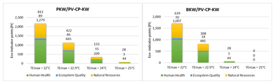
Figure 12.
Comparison of Eco-indicators of individual categories of damage for the analyzed variants.
In generalizing the values of the eco-indicators of the individual impact categories to broader categories of damage, it can be concluded that operating the proposed variants of air cooling systems primarily affects human health and natural resources, with a much lesser impact on the quality of the ecosystem. Human health is most affected by emissions of inorganic compounds and carcinogens associated with the substances used and, to a lesser extent, by climate change. With regard to natural resources, the main environmental burden is the consumption and extraction of fossil fuels.
Impact analysis under different assumptions of the maximum thermal comfort temperature shows a similar tendency towards decreasing impact in individual damage categories, as observed in impact categories. Any change in the assumed target value for cooling temperature results in a corresponding change in the level of impact on all analyzed damage categories.
It should be emphasized that the presented analysis only refers to the operational stage of the proposed installation variants, omitting the production, disassembly and final disposal stages of the equipment. Taking the full life cycle of the installation into account would result in higher Eco-indicator values and a greater estimated impact on the natural environment.
4.6. Economic Effect—LCC
An economic analysis of air cooling variants in the outdoor zone was carried out using the Life Cycle Cost (LCC) method. The calculations took into account the assumptions presented in Table 7.
Table 7.
Summary of energy carrier prices used to calculate the economic effect.
Unit prices of utilities are presented in Table 8.
Table 8.
Summary of assumptions used for the calculation of the economic effect.
The results of the life cycle cost analysis (LCC) showed differences between the individual variants of the outdoor air cooling system, depending on the assumed value of the upper limit of the cooling point (TEmax). Figure 13 shows the LCC values, which are calculated as the sum of acquisition costs and cost of ownership.
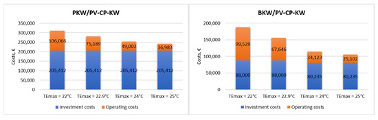
Figure 13.
The LCC value for different upper thermal comfort limits (TEmax) in two cooling system variants.
Investment costs for the indirect evaporative cooling variant (PKW/PV-CP-KW) remain unchanged regardless of the TEmax coefficient value adopted, as changes only affect the installation’s operating time and, consequently, operating costs. Operating costs decrease as the TEmax cooling endpoint value increases. In the case of the direct evaporative cooling variant (BKW/PV-CP-KW), however, an increase in investment costs is observed when the upper limit of thermal comfort exceeds TEmax = 24 °C. This is due to a decrease in demand for cooling and, consequently, a decrease in the required cooling capacity and number of devices (fewer evaporative air conditioners).
Operating costs are also showing a downward trend as the value of TEmax increases. The largest decrease (98%) was recorded in the range between TEmax = 22.9 °C and TEmax = 24 °C for the BKW/PV-CP-KW system. Increasing the cooling endpoint by 1.1 °C significantly improves the economic balance of the analyzed system and could be a cost-effective solution while only minimally reducing the thermal comfort quality standard.
4.7. Discussion of Results
This study uses a simplified comfort index, TE (effective temperature), which does not take into account radiation phenomena or the full impact of microclimatic conditions, which is a significant limitation when assessing thermal comfort in the outdoor environment. Although this model facilitates the energy assessment process, it does not allow for full generalization of the results to different climatic conditions. Therefore, the need to use a more comprehensive and proven index, such as the Universal Thermal Climate Index (UTCI), which is widely accepted in the literature and takes into account the impact of radiation, air velocity, and humidity on thermal comfort, has been emphasized.
Future research plans to monitor environmental parameters in a real building, which will allow for the verification of the adopted heat balance model and a comparison of the results obtained using the TE and UTCI indices. The analyzed facility remains available for recording the average radiation temperature, air temperature and humidity, and air flow intensity, which allows for experimental assessment of thermal comfort and calibration of models, thus increasing the reliability and practical usefulness of the results.
Sensitivity to water consumption and operational aspects is an important element in the evaluation of adiabatic cooling systems. In the analyzed solutions, water consumption is directly related to the demand for cooling and, thus, to meteorological conditions. A potential way to reduce water consumption is to use reclaimed water (e.g., gray water) or systems that support moisture recovery, which could reduce the operational impact, especially in conditions of elevated temperature and low humidity. In future studies, it will be useful to conduct a sensitivity analysis with regard to different scenarios of water source availability and quality.
An important factor affecting long-term energy self-sufficiency is the degradation of photovoltaic modules and the dependence of their efficiency on temperature. In this study, the energy analysis was carried out for the first year of operation, while the LCC economic analysis took into account a 1% annual decrease in module efficiency as a result of aging. In order to assess the degree of autonomy of the system in the long term, it will be necessary to directly take into account changes in PV efficiency as a function of temperature and usage time.
The results presented in this paper refer to simulation analyses of an evaporative cooling system powered by a local photovoltaic installation. To place our findings in a broader context, we compared them with available research. The results confirm the observations of other authors regarding the potential of PV and evaporative cooling systems to improve energy efficiency and reduce the demand for external power supply [25,42,61,62]. At the same time, LCA studies on solar and hybrid solutions indicate that the greatest environmental benefits are achieved when the assessment includes the operational phase and takes into account local electricity production profiles [62,63].
When comparing the results obtained with previous studies on evaporative cooling systems used outdoors, it should be emphasized that most of the work to date has focused on local scales (e.g., recreation areas, outdoor dining areas) or the use of individual cooling devices, while this analysis concerns a system integrated with public infrastructure and a local renewable energy source, which significantly affects the energy characteristics, mode of use, and potential energy autonomy.
Furthermore, the available literature lacks studies that simultaneously model thermal comfort in outdoor spaces and the degree of energy autonomy of the cooling system, which would allow for the identification of a compromise between these two objectives. Thus, the presented approach expands the existing body of knowledge, indicating the potential for improving thermal comfort in urban spaces with minimal energy consumption.
5. Conclusions
The research confirmed the high energy and economic efficiency of using air cooling systems in outdoor areas, powered by photovoltaic installations. The methodology developed enabled a detailed assessment of the impact of the upper limit of thermal comfort on the demand for useful, final and primary energy, as well as the degree to which these needs are met by the PV system.
The results of the analysis showed that increasing the TE index led to a reduction in energy consumption and an improvement in the efficiency of cooling systems. For the highest comfort limit analyzed (TEmax = 25 °C), the direct evaporative cooling system (BKW/PV-CP-KW) achieved full energy self-sufficiency, while the indirect system provided 97% coverage of demand.
Taking into account energy, economic, and environmental aspects, the most advantageous configuration was the direct evaporative cooling system at TEmax = 25 °C, which provided the highest degree of energy autonomy, minimal primary energy consumption (EP ≈ 0), and the lowest life cycle costs (LCC). These results confirm the possibility of creating autonomous, low-emission cooling systems based on renewable energy sources, which is a significant contribution to the development of sustainable technologies for outdoor spaces.
The proposed analytical model and the results obtained provide a reference point for the design of energy-efficient cooling systems powered by renewable energy. In further stages of the research, the model will be verified by measuring the average heat radiation temperature (for UTCI calculations) and analyzing the cooperation of the cooling system with electricity storage and PV cell cooling, which may further increase its autonomy and efficiency.
Author Contributions
Conceptualization, E.B., R.S., S.R. and J.D.-P.; methodology, E.B. and R.S.; software, E.B.; validation, E.B. and J.D.-P.; formal analysis, E.B. and R.S.; investigation, E.B.; resources, E.B., R.S., S.R. and J.D.-P.; data curation, E.B.; writing—original draft preparation, E.B.; writing—review and editing, E.B., R.S., S.R. and J.D.-P.; visualization, E.B. and R.S.; supervision, E.B.; project administration, E.B.; funding acquisition, S.R. All authors have read and agreed to the published version of the manuscript.
Funding
This research received no external funding.
Data Availability Statement
The original contributions presented in the study are included in the article; further inquiries can be directed to the corresponding author.
Conflicts of Interest
The authors declare no conflicts of interest.
Nomenclature
| A | study area (m2) |
| ci | correction factor depending on cooling system |
| d | annual degradation rate of PV cells (%) |
| Eel,pom,C | annual support final energy demand for cooling system (kWh year−1) |
| EK | annual final energy demand indicator (kWh m−2 year−1) |
| EP | annual primary energy demand indicator (kWh m−2 year−1) |
| EU | annual usable energy demand indicator (kWh m−2 year−1) |
| F | horizontal airflow area (m2) |
| H | height of study area (m) |
| hw | height of wind meter measurement (m) |
| hZ | height under study Z (m) |
| KN | capital costs (euro) |
| KP | ownership, operating costs (euro) |
| L | length of study area (m) |
| n | lifetime of installation (year) |
| N | number of photovoltaic modules (number) |
| No | number of people staying in study area |
| Pj | unit power of photovoltaic cell (W) |
| q | specific sensible heat (W person−1) |
| QCH | cooling power (kW) |
| QC,nd | annual utility energy demand for cooling (kWh year−1) |
| Qk | annual demand for non-renewable final energy supplied for technical systems (kWh year−1) |
| Qk,C | annual final energy demand for the cooling system (kWh year−1) |
| QL | heat gains from people (kWh) |
| Qu | annual useful energy demand (kWh year−1) |
| QZC | total heat gains for research facility (kWh) |
| QZC-S | constant heat gains calculated on the basis of heat balance (kWh) |
| QZC-Z | variable heat gains calculated on the basis of heat balance (kWh) |
| RH | relative humidity (%) |
| S | width of study area (m) |
| s | discount rate (%) |
| SEER | average seasonal coefficient of energy efficiency of cooling production |
| SEERref | reference average coefficient of energy efficiency of cold production |
| T | air temperature (°C) |
| T2 | real air temperature to be reached at cooling endpoint (°C) |
| TE | effective temperature (°C) |
| TEmax | upper limit of thermal comfort according to assumptions (°C) |
| V | volume of study object (m3) |
| w | wind velocity (m s−1) |
| wc | coefficient of non-renewable primary energy input for the generation and delivery of the energy carrier or energy for the cooling system |
| wel | coefficient of input of non-renewable primary energy for the generation and supply of electricity, specific for the annual auxiliary energy demand of the cooling system |
| ww | wind velocity at wind meter height (m s−1) |
| wZ | wind velocity at height Z (m s−1) |
| Z0 | aerodynamic roughness coefficient |
| mass flow rate (kg s−1) | |
| volume flow rate (m3s−1) | |
| Greek Symbols | |
| ηC,d | seasonal average efficiency of cooling distribution from cooling source to cooled area |
| ηC,e | average seasonal efficiency of control and usage of cooling in the cooled area |
| ηC,s | seasonal average cooling storage efficiency |
| ηC,tot | seasonal average total efficiency of cooling system |
| ϴ | length of period considered (year) |
| Abbreviations | |
| BKW/PV-CP-KW | a cooling system consisting of indirect evaporative air conditioners (local units), short ventilation ducts and air vents, combined with a photovoltaic installation |
| CP | cool air distribution |
| DEC | direct evaporative cooling |
| EC | heat energy |
| IEC | indirect evaporative cooling |
| KW | air diffuser |
| LCA | life cycle assessment (Pt) |
| LCC | life cycle cost (euro) |
| P1 | starting point of cooling process |
| P2 | endpoint of cooling process |
| PKW/PV-CP-KW | a cooling system comprising an indirect evaporative air conditioner (central unit) and ventilation ducts and air vents, combined with a photovoltaic installation |
| PV | photovoltaic cells |
| SEN | electricity grid |
| TRM | typical meteorological year |
| UHI | urban heat island |
References
- Bao, Y.; Li, Y.; Gu, J.; Shen, C.; Zhang, Y.; Deng, X.; Han, L.; Ran, J. Urban heat island impacts on mental health in middle-aged and older adults. Environ. Int. 2025, 199, 109470. [Google Scholar] [CrossRef] [PubMed]
- Avashia, V.; Garg, A.; Dholakia, H. Understanding temperature related health risk in context of urban land use changes. Landsc. Urban Plan. 2021, 212, 104107. [Google Scholar] [CrossRef]
- Hou, G.; Kuai, Y.; Yin, L.; Li, Y.; Shu, P. A comprehensive review of thermal comfort related design strategy of semi-outdoor transitional spaces. Energy Build. 2025, 345, 116116. [Google Scholar] [CrossRef]
- Jia, S.; Wang, Y.; Wong, N.H.; Weng, O. A hybrid framework for assessing outdoor thermal comfort in large-scale urban environments. Landsc. Urban Plan. 2025, 256, 105281. [Google Scholar] [CrossRef]
- Marando, F.; Heris, M.P.; Zulian, G.; Udías, A.; Mentaschi, L.; Chrysoulakis, N.; Parastatidis, D.; Maes, J. Urban heat island mitigation by green infrastructure in European Functional Urban Areas. Sustain. Cities Soc. 2022, 77, 103564. [Google Scholar] [CrossRef]
- Sayad, B.; Osra, O.A.; Binyassen, A.M.; Quattan, W.S. Analyzing Urban Climatic Shifts in Annaba City: Decadal Trends, Seasonal Variability and Extreme Weather Events. Atmosphere 2024, 15, 529. [Google Scholar] [CrossRef]
- Zhang, J.; Tu, L.; Wang, X.; Liang, W. Comparison of Urban Heat Island Differences in the Yangtze River Delta Urban Agglomerations Based on Different Urban–Rural Dichotomies. Remote Sens. 2024, 16, 3206. [Google Scholar] [CrossRef]
- Casson, N.; Cameron, L.; Mauro, I.; Friesen-Hughes, K.; Rocque, R. Perceptions of the health impacts of climate change among Canadians. BMC Public Health 2023, 23, 212. [Google Scholar] [CrossRef]
- Zhong, Y.; Li, S.; Liang, X.; Guan, Q. Causal inference of urban heat island effect and its spatial heterogeneity: A case study of Wuhan, China. Sustain. Cities Soc. 2024, 115, 105850. [Google Scholar] [CrossRef]
- Saez, R.A. Assessing the burdens of urban heat: A description of functional, economic and public health impacts of increasing heat in cities. In Policy Analysis; European University Institute: Fiesole, Italy, 2023; pp. 1–23. [Google Scholar] [CrossRef]
- Haeffelin, M.; Ribaud, J.F.; Céspedes, J.; Dupont, J.C.; Lemonsu, A.; Masson, V.; Nagel, T.; Kotthaus, S. Impact of boundary layer stability on urban park cooling effect intensity. EGUsphere 2024. [Google Scholar] [CrossRef]
- Zhu, Y.; Kensek, K.M. MITIGATING THE URBAN HEAT ISLAND EFFECT: The Thermal Performance of Shade-Tree Planting in Downtown Los Angeles. Sustainability 2024, 16, 8768. [Google Scholar] [CrossRef]
- Peng, L.L.H.; Jim, C.Y. Green-Roof Effects on Neighborhood Microclimate and Human Thermal Sensation. Energies 2013, 6, 598–618. [Google Scholar] [CrossRef]
- Bandurski, M.; Bandurska, H.; Kazimierczak-Grygiel, E.; Koczyk, H. The Green Structure for Outdoor Places in Dry, Hot Regions and Seasons—Providing Human Thermal Comfort in Sustainable Cities. Energies 2020, 13, 2755. [Google Scholar] [CrossRef]
- Pan, Y.; Li, S.; Tang, X. Investigation of Bus Shelters and Their Thermal Environment in Hot–Humid Areas—A Case Study in Guangzhou. Buildings 2024, 14, 2377. [Google Scholar] [CrossRef]
- Nicholson, S.; Nikolopoulou, M.; Watkins, R.; Love, M.; Ratti, C. Data driven design for urban street shading: Validation and application of ladybug tools as a design tool for outdoor thermal comfort. Urban Clim. 2024, 56, 102041. [Google Scholar] [CrossRef]
- Diem, P.K.; Nguyen, C.T.; Diem, N.K.; Diep, N.T.H.; Thao, P.T.B.; Hong, T.G.; Phan, T.N. Remote sensing for urban heat island research: Progress, current issues, and perspectives. Remote Sens. Appl. Soc. Environ. 2024, 33, 101081. [Google Scholar] [CrossRef]
- Babiarz, B.; Krawczyk, D.A.; Siuta-Olcha, A.; Manuel, C.D.; Jaworski, A.; Barnat, E.; Cholewa, T.; Sadowska, B.; Bocian, M.; Gnieciak, M.; et al. Energy Efficiency in Buildings: Toward Climate Neutrality. Energies 2024, 17, 4680. [Google Scholar] [CrossRef]
- Wei-Han, C.; Huai-En, M.; Tun-Ping, T. Performance improvement of a split air conditioner by using an energy saving device. Energy Build. 2018, 174, 380–387. [Google Scholar] [CrossRef]
- AL-Hasni, S.; Santori, G. The cost of manufacturing adsorption chillers. Therm. Sci. Eng. Prog. 2023, 39, 101685. [Google Scholar] [CrossRef]
- Halon, T.; Pelinska-Olko, E.; Szyc, M.; Zajaczkowski, B. Predicting Performance of a District Heat Powered Adsorption Chiller by Means of an Artificial Neural Network. Energies 2019, 12, 3328. [Google Scholar] [CrossRef]
- Evaporative Cooling Why It Is Perfect for Your Business. Available online: https://www.seeleyinternational.com/eu/commercial/evaporative-cooling-europe/ (accessed on 28 September 2025).
- Sajjad, U.; Abbas, N.; Hamid, K.; Abbas, S.; Hussain, I.; Ammar, S.M.; Sultan, M.; Ali, H.M.; Hussain, M.; Rehman, T.; et al. A review of recent advances in indirect evaporative cooling technology. Int. Commun. Heat Mass Transf. 2021, 122, 105140. [Google Scholar] [CrossRef]
- Mohammed, R.H.; El-Morsi, M.; Abdelazis, O. Indirect evaporative cooling for buildings: A comprehensive patents review. J. Build. Eng. 2022, 50, 104158. [Google Scholar] [CrossRef]
- Barnat, E.; Sekret, R.; Babiarz, B. Cooling of Air in Outdoor Areas of Human Habitation. Energies 2024, 17, 6303. [Google Scholar] [CrossRef]
- Haile, M.G.; Garay-Martinez, R.; Macarulla, A.M. Review of Evaporative Cooling Systems for Buildings in Hot and Dry Climates. Buildings 2024, 14, 3504. [Google Scholar] [CrossRef]
- Black-Ingersoll, F.; de Lange, J.; Heidari, L.; Negassa, A.; Botana, P.; Fabian, M.P.; Scammell, M.K. A Literature Review of Cooling Center, Misting Station, Cool Pavement, and Cool Roof Intervention Evaluations. Atmosphere 2022, 13, 1103. [Google Scholar] [CrossRef]
- Mortensen, K. Review of Evaporative Cooling’s Efficiency and Environmental Value. Ashrae J. 2022, 64, 55–61. Available online: https://spxcooling.com/wp-content/uploads/Review_Evaporative_Cooling_Efficiency.pdf?utm (accessed on 2 October 2025).
- Dhariwal, J.; Manandhar, P.; Bande, L.; Armstrong, P.; Reinhart, F.C. Evaluating the effectiveness of outdoor evaporative cooling in a hot, arid climate. Build. Environ. 2019, 150, 281–288. [Google Scholar] [CrossRef]
- Sonntag, D.B.; Jung, H.; Harline, R.P.; Peterson, T.C.; Willis, S.E.; Christensen, T.E.; Johnston, J.D. Infiltration of Outdoor PM2.5 Pollution into Homes with Evaporative Coolers in Utah County. Sustainability 2024, 16, 177. [Google Scholar] [CrossRef]
- Wei, Q.; Lu, J.; Xia, X.; Zhang, B.; Ying, X.; Li, L. Performance and Applicability Analysis of Indirect Evaporative Cooling Units in Data Centers Across Various Humidity Regions. Buildings 2024, 14, 3623. [Google Scholar] [CrossRef]
- Kostyák, A.; Szekeres, S.; Csáky, I. The Effect of Indirect Evaporative Cooling Applied to Existing AHU Systems. J. Archit. Eng. 2024, 30, 05024007. [Google Scholar] [CrossRef]
- Arunkumar, H.S.; Madhwesh, N.; Shenoy, S.; Kumar, S. Performance evaluation of an indirect-direct evaporative cooler using biomass-based packing material. Int. J. Sustain. Eng. 2024, 17, 1. [Google Scholar] [CrossRef]
- Wang, P.; Lu, S.; Wu, X.; Tian, J.; Li, N. Mist Spraying as an Outdoor Cooling Spot in Hot-Humid Areas: Effect of Ambient Environment and Impact on Short-Term Thermal Perception. Buildings 2024, 14, 336. [Google Scholar] [CrossRef]
- Solomon, G.M.; Martinez, N.; Behren, J.; Kaser, I.; Chang, D.; Singh, A.; Jarmul, S.; Miller, S.L.; Reynolds, P.; Heidarinejad, M.; et al. Evaporative coolers and wildfire smoke exposure: A climate justice issue in hot, dry regions. Front. Public Health 2025, 13, 1541053. [Google Scholar] [CrossRef] [PubMed]
- Zaki, A.M.; Bargal, M.H.S.; Antar, M.A.; Mokheimer, E.M.A.; Alhems, L.M. Advances in indirect evaporative cooling: Principles, integrated cycles, economic insights, and environmental implications. Therm. Sci. Eng. Prog. 2025, 67, 104078. [Google Scholar] [CrossRef]
- Stefaniak, Ł.; Szczęśniak, S.; Walaszczyk, J.; Rajski, K.; Piekarska, K.; Danielewicz, J. Challenges and future directions in evaporative cooling: Balancing sustainable cooling with microbial safety. Build. Environ. 2025, 267, 112292. [Google Scholar] [CrossRef]
- Romero-Lara, M.J.; Comino, F.; Ruiz de Adana, M. Seasonal energy efficiency ratio of regenerative indirect evaporative coolers—Simplified calculation method. Appl. Therm. Eng. 2023, 220, 119710. [Google Scholar] [CrossRef]
- Mihai, V.; Rusu, L. Improving the Ventilation of Machinery Spaces with Direct Adiabatic Cooling System. Inventions 2022, 7, 78. [Google Scholar] [CrossRef]
- Parker, D.; Panchabikesan, K.; Dagostiono, D.; Crawley, D.B.; Lawrire, L. Coincidence of Photovoltaic Electric Generation During Heat Waves: An Example Analysis for Northern Italy. In Proceedings of the 41st European Photovoltaic Solar Energy Conference and Exhibition EU PVSEC 2024, Vienna, Austria, 23–27 September 2024; pp. 020562-001–020562-003. [Google Scholar] [CrossRef]
- Kan, X.; Hedenus, F.; Reichenberg, L.; Hohmeyer, O. Into a cooler future with electricity generated from solar photovoltaic. iScience 2022, 25, 104208. [Google Scholar] [CrossRef]
- Xue, T.; Wan, Y.; Huang, Z.; Chen, P.; Lin, J.; Chen, W.; Liu, H. Comprehensive Review of the Applications of Hybrid Evaporative Cooling and Solar Energy Source Systems. Sustainability 2023, 15, 16907. [Google Scholar] [CrossRef]
- Ghosh, P.; Wei, X.; Liu, H.; Zhang, Z.; Zhu, L. Simultaneous subambient daytime radiative cooling and photovoltaic power eneration from the same area. Cell Rep. Phys. Sci. 2024, 5, 101876. [Google Scholar] [CrossRef]
- Strobel, M.; Jakob, U.; Streicher, W.; Neyer, D. Spatial Distribution of Future Demand for Space Cooling Applications and Potential of Solar Thermal Cooling Systems. Sustainability 2023, 15, 9486. [Google Scholar] [CrossRef]
- Khan, A.; Anand, P.; Garshasbi, S.; Khatun, R.; Khorat, S.; Hamdi, R.; Niyogi, D.; Santamouris, M. Rooftop photovoltaic solar panels warm up and cool down cities. Nat. Cities 2024, 1, 780–790. [Google Scholar] [CrossRef]
- Institute of Meteorology and Water Management, Institute of Meteorology and Water Management-State Research Institute. Available online: https://www.imgw.pl/ (accessed on 10 October 2022).
- Freitas, C.R.; Grigorieva, E.A. A comprehensive catalogue and classification of human thermal climate indices. Int. J. Biometeorol. 2015, 59, 109–120. [Google Scholar] [CrossRef]
- Błażejczyk, K. Bioklimatyczne Uwarunkowania Rekreacji i Turystyki w Polsce. Warszawa 2004. Available online: https://rcin.org.pl/igipz/Content/19801/PDF/WA51_39725_r2011-nr13_Monografie.pdf (accessed on 2 October 2025). (In Polish).
- Błażejczyk, K. UTCI—10 years of applications. Int. J. Biometeorol. 2021, 65, 1461–1462. [Google Scholar] [CrossRef]
- Höppe, P. The physiological equivalent temperature—A universal index for the biometeorological assessment of the thermal environment. Int. J. Biometeorol. 1999, 43, 71–75. [Google Scholar] [CrossRef]
- Ambrsio Alfano, F.R.; Palella, B.I. Thermal Environment Assessment Reliability Using Temperature—Humidity Indices. Ind. Health 2011, 49, 95–106. [Google Scholar] [CrossRef]
- Klemm, K. Wind flow in an urban area and opportunities for its use. Pol. Sol. Energy 2010, 4, 37–42. [Google Scholar]
- Strzelczyk, P.; Szczerba, Z.; Wozniak, A. Vertical modelling of the wind speed profile in an aerodynamic model. JCEEA 2015, 32, 413–427. [Google Scholar] [CrossRef]
- Regulation of the Minister of Infrastructure and Development of 27 February 2015 on the Methodology for Determining the Energy Performance of a Building or Part of a Building and Energy Performance Certificates. Journal of Laws of 18 March 2015, item 376, as Amended. Available online: https://isap.sejm.gov.pl/isap.nsf/DocDetails.xsp?id=WDU20150000376 (accessed on 15 October 2024). (In Polish)
- PN-EN ISO 14040:2009; Environmental Management—Life Cycle Assessment—Principles and Structure. ISO: Geneva, Switzerland, 2009. (In Polish)
- PN-EN ISO 14044:2009; Environmental Management—Life Cycle Assessment—Requirements and Guidelines. ISO: Geneva, Switzerland, 2009. (In Polish)
- Sekret, R. Environmental aspects of energy supply of buildings in Poland. In E3S Web of Conferences; EDP Sciences: Les Ulis, France, 2018; p. 49. [Google Scholar] [CrossRef]
- Sekret, R. Evaluation of environmental impact on selected heat supply systems of buildings for energy management. Rynek Energii 2019, 1, 48–55. [Google Scholar]
- Bogusz, A. LCC Life Cycle Costs Repository. Efficient public procurement. In Polish, Katowice, Poland 2022. Available online: https://dzp.us.edu.pl/wp-content/uploads/2025/01/Repozytorium-koszty-cyklu-zycia-LCC.pdf (accessed on 15 October 2024).
- Bogusz, A.; Polakowski, Ł. Life cycle cost accounting—LCC. In Green Public Procurement—II Handbook; Skowron, M., Ed.; Public Procurement Office: Warsaw, Poland, 2012. [Google Scholar]
- El Kassar, R.; Al Takash, A.; El Raasy, E.; Hammoud, M.; Py, H. Photovoltaic cooling systems review integrating technical, economic, and environmental dimensions encompassing life cycle assessment. Sol. Energy 2025, 302, 114010. [Google Scholar] [CrossRef]
- Finocchiaro, P.; Beccali, M.; Cellura, M.; Guarino, F.; Longo, S. Life Cycle Assessment of a compact Desiccant Evaporative Cooling system: The case study of the “Freescoo”. Sol. Energy Mater. Sol. Cells 2016, 156, 83–91. [Google Scholar] [CrossRef]
- Frischknecht, R.; Stolz, P.; Krebs, L.; de Wild-Scholten, M.; Sinha, P. Life Cycle Inventories and Life Cycle Assessments of Photovoltaic Systems 2020; Report IEA-PVPS T12-19:2020; International Energy Agency: Paris, France, 2020; Available online: https://iea-pvps.org/wp-content/uploads/2020/12/IEA-PVPS-LCI-report-2020.pdf (accessed on 4 October 2025).


Disclaimer/Publisher’s Note: The statements, opinions and data contained in all publications are solely those of the individual author(s) and contributor(s) and not of MDPI and/or the editor(s). MDPI and/or the editor(s) disclaim responsibility for any injury to people or property resulting from any ideas, methods, instructions or products referred to in the content. |
© 2025 by the authors. Licensee MDPI, Basel, Switzerland. This article is an open access article distributed under the terms and conditions of the Creative Commons Attribution (CC BY) license (https://creativecommons.org/licenses/by/4.0/).