LoRaWAN Gateway Placement in Smart Agriculture: An Analysis of Clustering Algorithms and Performance Metrics

Abstract

The use of Wireless Sensor Networks (WSN) in smart agriculture has emerged in recent years. LoRaWAN (Long Range Wide Area Networks) is widely recognized as one of the most suitable technologies for this application, due to its capacity to transmit data over long distances while consuming little energy. Determining the number and location of gateways (GWs) in a production setting is one of the most challenging tasks of planning and building this type of network. Various solutions to the LoRaWAN gateway placement problem have been proposed in the literature, utilizing clustering algorithms; however, few works have compared the performance of various strategies. Considering all these facts, this paper proposes a strategy for planning the number and localization of LoRaWAN GWs, to cover a vast agricultural region. Four clustering algorithms were used to deploy the network GWs: K-Means and its three versions: Minibatch K-Means; Bisecting K-Means; and Fuzzy c-Means (FCM). As performance metrics, uplink delivery rate (ULDR) and energy consumption were used, to provide subsidies for the network designer and the client, with which to choose the best setup. A stochastic energy model was used to evaluate power consumption. Simulations were performed, considering two scenarios: Scenario 1 with lower-medium concurrence, and Scenario 2 with higher-medium concurrence. The simulations showed that the use of more than two GWs in Scenario 1 did not lead to significant improvements in ULDR and energy consumption, whereas, in Scenario 2, the suggested number of GWs was between 11 and 15. The results showed that for Scenario 1, the FCM algorithm was superior to all alternatives, regarding the ULDR and mean energy consumption, while the K-Means algorithm was superior with respect to maximum energy consumption. In relation to Scenario 2, K-Means caused the best ULDR and mean consumption, while FCM produced the lowest maximum consumption.

1. Introduction

The global population expansion, the reduction of natural resources and cropland area, and unpredictable weather patterns have resulted in a significant challenge to ensuring food accessibility [1]. Considering these challenges, the agricultural industry has begun to adopt technology as a means of increasing efficiency and productivity. The use of the IoT (Internet of Things) and big data has become prevalent in this context. WSNs are a fundamental aspect of those systems, as they provide farmers with vital information about soil conditions, crop growth, and animal behavior, thus enabling them to make more informed decisions [2]. In addition to food availability, the problem of water pollution caused by agriculture can lead to negative impacts on the environment and on human health, and the use of a WSN can help to solve this issue [3]. The IoT ecosystem comprises various components, including sensors, actuators, smartphones, automobiles, personal computers, and cameras. It is anticipated that the IoT will continue to benefit a wide range of industries, including transportation, manufacturing, and healthcare, for the foreseeable future [4].

Limited-power Wide Area Network (LPWAN) is a type of WSN technology that enables the connection of battery-powered devices with low bandwidth and low bit rate over extended distances. The most well-known LPWAN protocols include Narrowband IoT (NB-IoT), Sigfox, and LoRaWAN [5]. This study focused on LoRaWAN, a protocol specifically designed to meet the critical requirements of the IoT, such as bidirectional communication, end-to-end security, mobility, and location services. LoRaWAN was developed to wirelessly connect devices in regional, national, and global networks to the internet, in order to provide coverage over a vast area, while consuming minimal energy [6].

In LoRaWAN, GWs act as the intermediary between LoRaWAN end-devices (EDs) and the network server (NS), utilizing communication technologies such as WiFi, Ethernet, and cellular. Meanwhile, EDs connect to the GWs using the LoRa (Long Range) protocol [7]. The coverage, collision probability, and power consumption of the network are contingent on the number and positioning of the GWs, as the transmission power of the EDs is relatively high. A network with inadequate or poorly positioned GWs will likely experience increased collisions, communication failures, and energy consumption. Furthermore, the power consumption of sensors, actuators, and radios can be significant, making the design of algorithms for energy-saving and power circuitry—including the selection of batteries and solar panels—a topic of ongoing research and debate in the scientific community [8,9].

Clustering is a promising method for determining the number and placement of GWs: it has been used in WSNs to improve network scalability, reduce energy consumption, and increase data reliability [10]. There are many types of clustering techniques that are classified as hierarchical, centroid-based, density-based, and distribution based. Hierarchical clustering is suitable for grouping similar items together, as it generates cluster trees. This type of clustering can be divided into two main methods: agglomerative and divisive. Agglomerative clustering combines clusters, to form hierarchical groups, using a bottom-up approach. Divisive clustering breaks down clusters into smaller groups, using a top-down approach. Centroid-based clustering employs center vectors to identify each cluster, and assigns items to the closest cluster center, to minimize squared distances. Density-based clustering forms clusters from areas with a high concentration of occurrences. Distribution-based clustering uses the distance from the probability distribution center, to determine the likelihood of an item belonging to a particular cluster. K-Means, a centroid-based method, is commonly used to solve cluster formation in WSNs [11]. In addition to K-Means, there are three variations of it: Minibatch K-Means; Bisecting K-Means; and FCM.

End-users primarily value a communication system on the basis of its reliability and cost [12]: with this in mind, this research presents new and promising results for planning LoRaWAN in smart agriculture IoT applications. Various scenarios were established in a large agricultural area located in Petrolina, one of the most productive fruit-growing cities in Brazil. By using the proposed method, designers can plan and evaluate the performance and behavior of WSNs, and make informed decisions on the parameters during the design process.

In this article, a method for placing LoRaWAN GWs in smart agriculture applications, using K-Means and its three variations, is proposed. The method is comprised of five phases: (1) characterization of the environment, including delimiting the plantation area, and modeling and parameterizing RF (Radio Frequency) signal propagation; (2) calculation of LoRaWAN GW location, using K-Means and its three variants, taking into account the positions of the EDs; (3) simulation of network performance, using LoRaWANSim (a free and open-source simulator [13]) for various GW setups, up to the maximum number of GWs; (4) statistical analysis of the performance of all simulations; (5) selection of the best GW setup, based on performance results. Additionally, we propose the use of a stochastic energy model, to evaluate the power consumption performance of the WSN. The ULDR, mean, maximum, and minimum ED energy consumption levels were also used, to support the final deployment decision.

This paper presents five contributions to the field of LoRaWAN technology: (1) the use of a stochastic energy model to determine the optimal interval of GW numbers (as developed in previously published work), in order to minimize the energy consumption of LoRaWAN radios in all operation modes; (2) the testing of four different clustering algorithms, to determine the optimal GW locations and numbers, using the energy model and ULDR as a parameter; (3) a comprehensive characterization of the environment, focusing on a real polygonal plantation area in one of Brazil’s most fruit-productive regions; (4) a comparison of the proposed method under different levels of medium-access concurrence; (5) presentation of novel simulation results that provide insight into the performance of LoRaWAN and the impact of various configurations.

The organization of this paper is as follows: Section 2 provides background information on LoRa and LoRaWAN technologies, delves into the basics of clustering, and highlights the current state of the art; Section 3 details the performance measurements and methodology used in this study; Section 4 presents the results obtained by the simulator, and compares them to the energy model and metrics; Section 5 concludes with a summary of the findings, and suggestions for future research.

2. Literature Review and Related Work

This section presents the main concepts related to LoRa and LoRaWAN, the clustering algorithms used in this work, and the related work.

2.1. LoRa and LoRaWAN

At the physical layer (PHY), LoRa uses the M-ary Chirp Spread Spectrum (MCSS) modulation technique, which involves the transmission of sine-wave signals that linearly sweep its frequency. One of the key features of LoRa is the ability to adjust the spreading factor (SF) of the signal. The SF is a value that determines the amount of spreading that is applied to the signal before it is transmitted. Higher SF values result in a wider frequency spread of the signal, which in turn improves the communication range, robustness against channel impairments and third-party interference, frequency selectivity, and resilience to the Doppler effect; however, it is important to note that increasing the SF reduces the data rate, and increases the wireless channel transmission time (ToA): this trade-off is particularly important in LoRaWAN, in which the SF is a key parameter that must be considered when designing and deploying the network. Additionally, the LoRa modulation technique is designed to work in the industrial, scientific, and medical (ISM) bands, which are unlicensed frequency bands that are available for use by anyone, without the need for a license, thus making LoRa an attractive option [14].

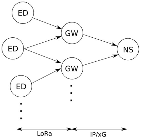
LoRaWAN is a networking protocol that extends the LoRa physical layer (PHY) protocol, by adding additional layers of functionality. The most common design for LoRaWAN is a star-of-stars topology, so that EDs communicate with GWs using LoRa, and the GWs, in turn, connect to an NS using Internet Protocol (IP) connections, such as Wi-Fi, Ethernet, or cellular networks (3G/4G/5G-xG) (Figure 1) [15].

Figure 1. LoRaWAN topology diagram.

The NS acts as a central point for the LoRaWAN network, being responsible for several key functions. The NS discards duplicate messages, to prevent data from being processed multiple times, sends acknowledgments (ACKs) to the EDs, to confirm that their messages have been received, and controls the data flow from the GWs, to ensure that the network remains stable and secure. In addition, the NS also performs several other functions, such as managing the connection between the EDs and GWs, allocating communication channels, and managing the overall network topology. The NS also performs security functions, such as encryption, authentication, and authorization of devices in the network. Furthermore, the NS manages access to the network by multiple EDs and GWs, providing a secure and scalable network infrastructure [16].

The LoRaWAN standard classifies devices into three classes: Class A, Class B, and Class C. Each device class has different characteristics, and is suited to different types of applications. Class A devices are designed for low-power applications, and have the ability to receive downlink messages on RX1 and RX2 windows. Class A devices are typically used in applications in which power consumption is a critical concern, and have a sleep time between transmissions. Class B devices have a more complex receiving schedule, and require end-device-gateway synchronization. Class B devices are typically used in applications that require a higher level of responsiveness, and have more frequent transmissions. Class C devices have one continuous waiting slot, which allows them to receive downlink messages at any time. Class C devices have the highest power consumption, and are best-suited to applications that require a high level of connectivity, and low latency [17].

In addition to the different classes of devices, LoRaWAN also supports two different modes of operation: confirmed and unconfirmed. In the confirmed mode, the NS sends an ACK packet to the ED, for each packet that is successfully delivered: this ensures that the ED knows that the packet has been received, and can take appropriate action if necessary. In unconfirmed mode, the NS does not send an ACK packet, which reduces the overhead of the network, but also increases the risk of lost packets [18].

Furthermore, the LoRaWAN protocol is designed to be highly scalable, enabling the deployment of networks that can support thousands of devices. This scalability is achieved through the use of adaptive data rate (ADR) algorithms, which dynamically adjust the ED transmission parameters (SF and transmission power, $P_t$). The NS records the device’s uplink broadcasts’ frame counter, signal-to-noise ratio (SNR), and the number of GWs that receive each frame when the ADR is set. After 20 transmissions, the algorithm iterates, depending on the maximum SNR, and provides the SF and $P_t$ to the EDs [19].

2.2. Clustering Techniques

Clustering is a data mining technique that is used to divide a dataset into groups, or clusters, of similar data points. The goal of clustering is to find natural patterns, or groupings, in the data that optimize one or more metrics, without any prior knowledge of the underlying structure. Clustering algorithms can be either hard or soft. Hard clustering algorithms assign each data point to a single cluster, while soft clustering algorithms assign each data point to multiple clusters with different membership degrees. The clustering structure is represented as a collection of subsets $C=C_1,\dots ,C_K$ of S, such that $S={\bigcup }_{i=1}^K{C}_i$. The number of clusters, K, is a user-defined parameter that is determined prior to the algorithm running, or is obtained when a stop criterion is met. To evaluate whether two elements of the set are similar or not, one or more metrics are required: these metrics are used to compute the similarity or dissimilarity between data points. Common metrics used in clustering include Euclidean distance, Manhattan distance, Cosine similarity, and Jaccard similarity. The choice of metric will depend on the characteristics of the dataset, and the specific requirements of the application [20].

K-Means is a popular and widely used clustering algorithm that partitions a dataset into a specified number of clusters, based on their similarity [21]. The algorithm works by iteratively assigning each data point to the cluster whose centroid is closest to it, and then re-calculating the centroid of each cluster as the mean of all points assigned to that cluster. The process is repeated until the assignment of points to clusters no longer changes, or until a stopping criterion is met. K-Means clusters data by minimizing the inertia or within-cluster sum-of-squares, to divide samples into n groups. This algorithm requires the cluster number, and separates N samples into K distinct clusters, each with a mean ${\mu }_j$. The cluster centroids are not points of S. The inertia can be obtained by:

$$I=\sum _{i=0}^N\underset{{\mu }_j\in C}{min}\left({∥x_i-{\mu }_j∥}^2\right),$$

in which $x_i$ represents the values of the features or attributes for the ith observation in the dataset.

The algorithm is founded on the concept of Voronoi diagrams, in which the initial centroid positions are used to calculate the Voronoi diagram of the points. In a second phase, the segment means are used to update the centroids. The algorithm repeats this, until it meets a stopping requirement. The method usually finishes when the relative drop in the objective function between iterations is less than the tolerance value.

MiniBatch K-Means is a variation of the traditional K-Means clustering algorithm that is designed to minimize computation time while still optimizing the same objective function [21]. The algorithm consists of two major phases: (1) a mini-batch of samples is created by randomly selecting a subset of the dataset, which is then assigned to the nearest centroid; (2) the allocated centroid is updated by taking the average of each mini-batch sample and all previous samples associated with that centroid. The process is repeated until convergence or a predefined number of iterations. According to the literature, MiniBatch K-Means is known to converge faster than K-Means; however, it is also known to produce lower-quality results: this is because the random sampling of the dataset in MiniBatch K-Means can result in less accurate centroid estimates, and can cause the algorithm to converge to a local minimum. To address this issue, several variations of MiniBatch K-Means have been proposed, such as using a larger mini-batch size or using a different sampling method to improve the quality of the results.

The iterative Bisecting K-Means is a variation of the traditional K-Means algorithm, and uses a divisive hierarchical clustering approach [21]. Instead of starting with a predefined number of clusters, and trying to optimize the cluster assignments and centroids, the Bisecting K-Means algorithm starts with all data points in a single cluster, and then repeatedly splits the largest cluster into two smaller clusters, until the desired number of clusters is reached. One of the main advantages of the Bisecting K-Means algorithm is that it is more efficient than traditional K-Means when the number of clusters is large: this is because it only works on a subset of the data at each bisection, rather than the complete dataset, which can make it a more suitable option for datasets with a large number of clusters or a large number of data points. Another advantage of Bisecting K-Means is that it is less sensitive to the initial placement of centroids, and it can also be used when the data are not clearly separable or when the clusters have different sizes.

FCM is a soft clustering algorithm that allows each data point to belong to multiple clusters, based on its probability score or likelihood [22]. In contrast to hard clustering techniques, such as K-Means, MiniBatch K-Means, and bisecting K-Means—in which each data point is assigned to one cluster only—FCM uses a probability-based approach, in which each data point is assigned a degree of membership to each cluster, between 0 and 1. In FCM, the objective function is to minimize the within-cluster sum-of-squares, similarly to K-Means, but with an additional term in the objective function that assigns a degree of membership to each data point. The membership of each point is determined by its distance to the center of each cluster. Points located closer to cluster centers have a higher membership than those located closer to cluster edges. One of the main advantages of FCM is that it can handle data that do not clearly belong to a single cluster, which can be the case in many real-world applications. Additionally, it is less sensitive to the initial placement of centroids, compared to hard clustering algorithms.

The basic diagram for the clustering methods is shown in Figure 2. The coordinates of the EDs and the number of clusters are the inputs for solving the problem of locating GWs in the LoRaWAN network; the outputs are the centroids of the clusters, and labels for each device, which identify the cluster to which it belongs.

Figure 2. Diagram which illustrates the main inputs and outputs of the clustering algorithms.

2.3. Related Work

Feltrin et al. [23] have highlighted the potential of LoRaWAN technology for IoT applications in large areas. Through a combination of laboratory and field experiments, the authors provided a link-level characterization of LoRaWAN technology. Additionally, a system-level simulation was conducted, to evaluate the capacity of a single LoRaWAN GW and a network of multiple GWs to service a large area. The simulation results showed that the use of multiple GWs can significantly increase the network capacity and delivery rate. In a separate study, Miles et al. [24] analyzed the performance of LoRaWAN communication networks in an IoT application for a pilot farm. The authors used simulations to analyze various scenarios, and to provide a mathematical model with which to predict the packet delivery rate of the network, based on the number of nodes and the transmission interval duration. In another research, Kamonkusonman et al. [25] proposed a Utilization-Weighted (UW) SF assignment technique, to improve the scalability of LoRaWAN for dairy farms. The proposed algorithm was compared to the traditional approach on the packet delivery rate and energy usage. The results showed that the UW algorithm had a greater packet delivery ratio without sacrificing energy usage. In Ref. [26], a data acquisition system that used a hybrid communication network, based on LoRa modules, was presented. A hydraulic plant was selected, to test the proposed system. Yascaribay et al. [27] presented a method for evaluating IoT communication systems for agriculture, based on parameters such as packet delivery ratio, energy usage, and packet collisions. The researchers compared the performance of LoRa and LoRaWAN in a rural coastal Ecuadorian scenario, and examined the package delivery ratio and energy consumption. The work in [28] used Multilayer Perceptron (MLP) neural networks to predict plant growth, based on the RSSI indicator. Neural network training was carried out, based on the collection of data from sensors in several chambers of a greenhouse. The results of the developed method illustrated a good prediction of plant height with the help of RSSI values.

A study by [29] addressed the optimal deployment of LPWAN IoT GWs. The authors proposed two different GW deployment methods: network-aware and network-agnostic. In network-aware GW deployment, the locations of the IoT EDs are precisely known, whereas in network-agnostic GW deployment, the locations of the EDs are not required. The authors used K-Means clustering to determine the optimal location of GWs in network-aware deployment, and demonstrated that using computational methods for GW placement can lead to competitive network performance, while reducing network expenses and enhancing sustainability. In Ref. [30], the Naive Bayes algorithm was used to improve message scheduling in LoRaWAN, while the K-Means algorithm was used for cluster formation, as being the basis technique. Matni et al. [31] developed a GW placement method called DPLACE, which used FCM clustering and Gap statistics, to assess the cluster size and to determine the optimal positions for LoRaWAN GWs. The goal of the method was to lower costs while maintaining high Quality of Service (QoS). In another research, Mendes et al. [32] proposed an optimization model that minimized power consumption by critical equipment, based on packet delivery, and could be used to schedule GW position changes to extend network lifetime. The results suggested that the optimization model and the proposed pipeline were suitable for planning wide area monitoring, and could predict GW rearrangements to extend network lifetime. Cruz et al. [33] provided an empirical and statistical methodology based on measurements, in a typical Amazonian city with a mix of woods and buildings, to adjust the coefficients in the propagation model. The authors used an Evolutionary Particle Swarm Optimization (EPSO) metaheuristic with multi-objective optimization to maximize coverage and minimize GWs for LoRa network planning.

3. Materials and Methods

This section presents the metrics used to evaluate the WSN performance, the characteristics of the environment, the simulation parameters, and the method that was used to plan and evaluate the simulation results.

3.1. Uplink Delivery Rate

In LoRaWAN, noise and interference cause packets to be wrongly received by the GWs. A reliable system receives every packet and keeps track of the transmitter’s messages and the base station’s received messages, so as to determine reliability [13]. The ULDR or percentage of signals received is defined as the reliability of the network, and is given by

$$\upsilon =\frac{{\varphi }_r}{{\varphi }_t},$$

in which ${\varphi }_r$ and ${\varphi }_t$ are the numbers of packets transmitted and received, respectively. This metric allows for system comparison, regardless of technology.

3.2. Energy Consumption Model

Real EDs have minimum and maximum power consumption limits. Ideally, all network nodes would consume the minimum: however, due to random factors that vary power usage (e.g. node position, antenna gain variation, temperature, SF, optimization algorithms, collisions), this is unattainable. If energy consumption is near the lowest limit, a WSN can be called well-designed. The stochastic energy model used in this work considered these facts, and was proposed in [34]. The probability density function (PDF) of the energy consumed per cycle was obtained by the PDFs of each state convolution, which was given by

$$\begin{array}{c}\hfill p_E\left(e\right)=\sum _{i=1}^M\frac{{\beta }_1···{\beta }_n}{{\displaystyle \prod _{\begin{array}{c}j=1\\ j\ne i\end{array}}^M}({\beta }_j-{\beta }_i)}exp[-{\beta }_{i}e]u\left(e\right),\end{array}$$

(1)

in which ${\beta }_k={\alpha }_k/\overline{{\psi }_k}$, ${\alpha }_k$ is the inverse of the time in a state k average, and $\overline{{\psi }_k}$ is the average consumed power. Using the ADR algorithm, the NS managed the SF and $P_t$ of the EDs in the LoRaWAN network. The ADR optimizes the transmission rate and the power consumption. Most NSs follow Semtech suggestion [35], even though LoRaWAN does not specify it. The NS collects the uplink (UL) packet signal to noise ratio (SNR) information, how many GWs received each uplink packet, $P_t$, and the SF of the EDs. The SF choice influences the transmission and reception window size, which affects the ToA and device state duration. Medium access unpredictability and reception window utilization affect sleep and idle time. Therefore, the variability of power consumption is caused mainly due to the ADR algorithm, and this energy model captured this behavior.

Real radios have energy consumption constraints because of their hardware, firmware, and application setup characteristics. The model had to account for the device’s minimum threshold, which is usually non-zero. The change of basis could be utilized to shift every statement supplied in coordinates of one basis into another, as Equation (1) did not address this limit. Consequently, all the model parameters had to be transposed to the origin (coordinates $(0,0)$), the model curve was computed, then it was shifted to the right, $p_E\left(e\right)=p_E{(e-E_{c_{min}})}^{{}^{\prime }}$ [34].

3.3. Environment Characterization

The Nilo Coelho Project is part of the Petrolina/Juazeiro irrigation complex in Brazil [36], and began operations in 1984, occupying an area that extends along the São Francisco River. This project covered an irrigable surface occupied by small producers and by small, medium, and large companies, subdivided into areas called PA I, II, and III, and Maria Tereza. The planted area of the Maria Tereza project is around 100 km², and was chosen to carry out the planning of the network. With a predominance of fruit growing, in 2021, the grape crop participated in the production of 70%, mango 13%, guava 7%, acerola 4%, and other crops with 6%.

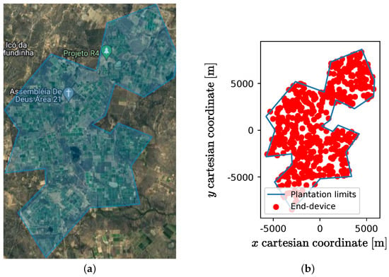
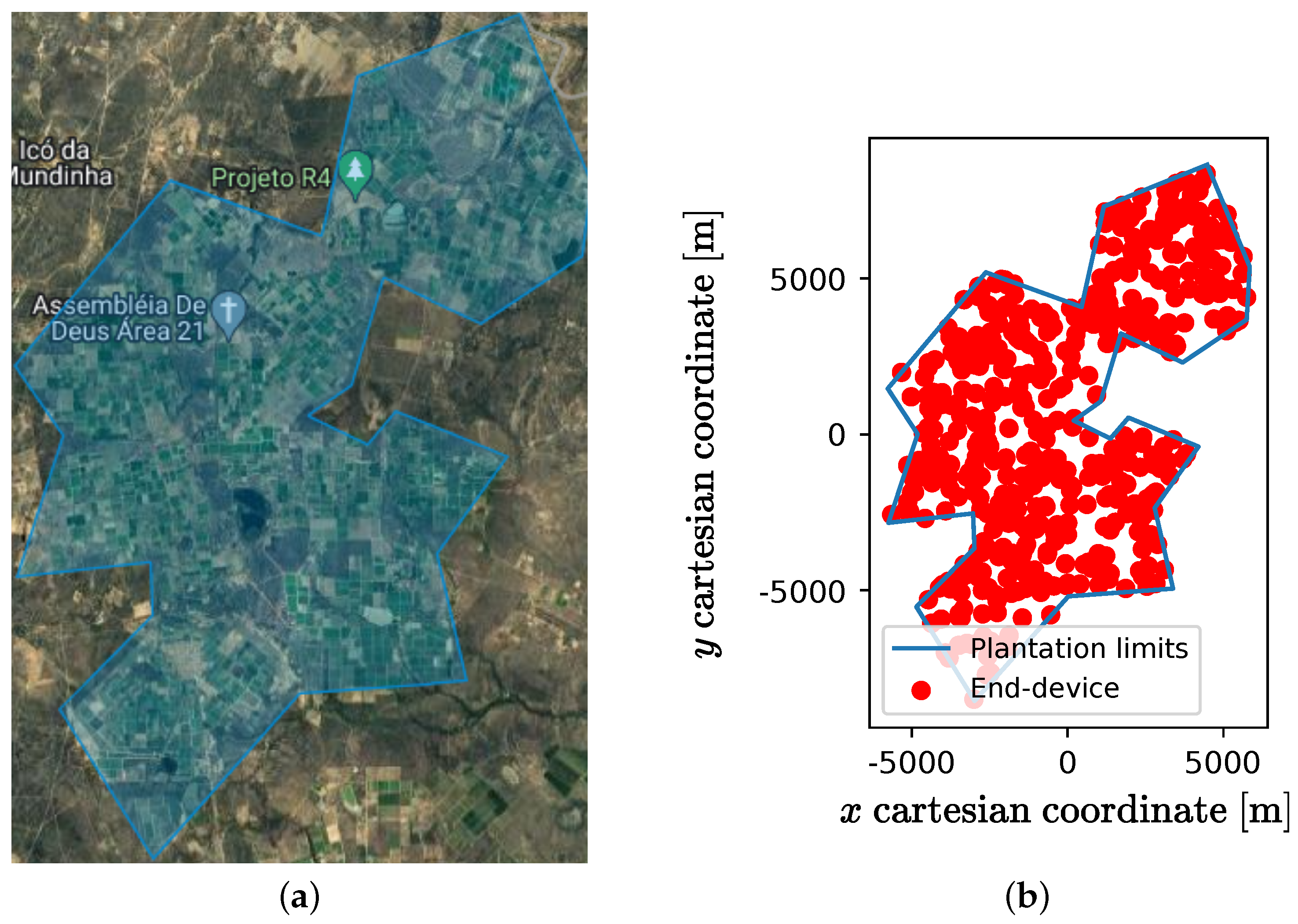
To fill in the map data in the simulator (read Section 3.4), it was necessary to carry out a projection of the map, considering that the simulator used the Cartesian coordinate system: this was done with the Inkscape software, so that the scaled-down distances between the extreme points on the map were the same as those measured on Google Earth. Figure 3 presents a screen capture of the studied region, as well as the projection of the map in the Cartesian system.

Figure 3. (a) Google Earth screen capture of the Nilo Coelho Project irrigation complex in Brazil, and (b) its projection to Cartesian coordinates.

The log-distance propagation model—also known as the log-normal shadowing model—is a commonly used model for predicting the propagation and attenuation of radio signals as they travel through the environment. It is based on the assumption that the propagation loss is a log-normal random variable, and that the mean of this variable varies with distance, according to a power-law relationship. The log-distance propagation model is flexible, meaning that it can be used to predict propagation loss for various situations, including both line-of-sight and non-line-of-sight scenarios. In line-of-sight scenarios, the signal travels directly from the transmitter to the receiver without encountering any obstacles, while in non-line-of-sight scenarios, the signal encounters obstacles, such as buildings, trees, and other structures that can cause signal loss [37]. Despite it is a simple classic model, all details of the propagation environment are dealt with by the Radio Mobile simulation software [38]. The formulation of the model was given by

$$\begin{array}{c}\hfill P_r=P_t+G_t+G_r-10nlog\left(d\right)+X_{\sigma },\end{array}$$

(2)

in which $P_r$ was the received signal power and $P_t$ was the transmission power. The parameters $G_t$ and $G_r$ were the gains of the transmitting and receiving antennas, and d was the distance between the devices. The variable $X_{\sigma }$ refers to the shadow fading or log-normal fading component of the received signal power. Shadow fading is a type of signal attenuation caused by obstructions such as buildings, trees, and terrain. It is a random variable that follows a log-normal distribution with zero mean and standard deviation $\sigma$.

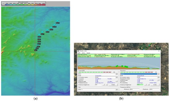
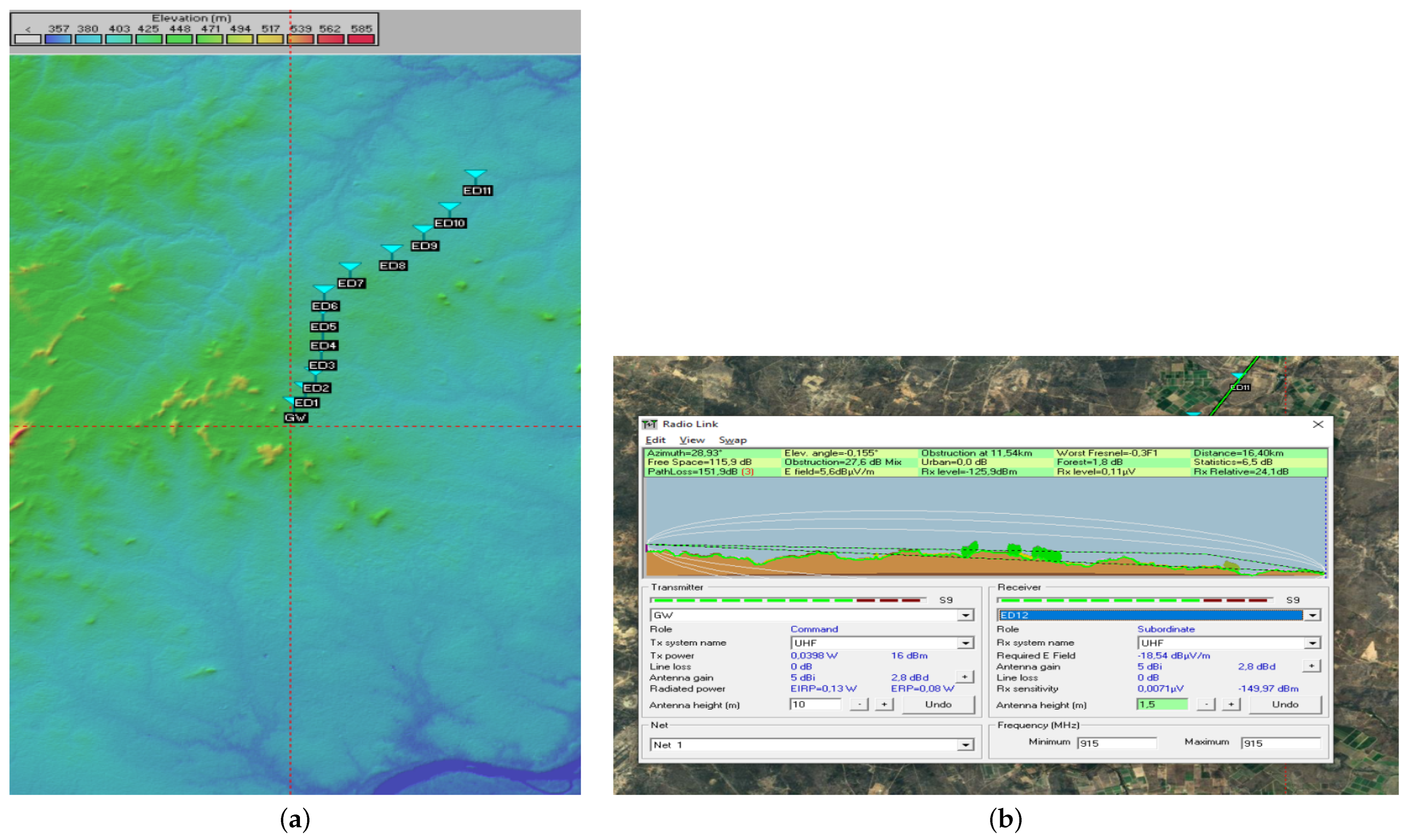
To obtain the parameter n of the model, the Radio Mobile software was used. The program is a free radio propagation simulator that operates in the frequency range from 20 MHz to 20 GHz, and uses digital terrain elevation data for automatic extraction of the path profile between an emitter and a receiver. The simulation parameters used in the Radio Mobile software are shown in Table 1. Figure 4 shows a screenshot of the software, and the map points that were used in the simulation.

Table 1. Radio Mobile input parameters.

Parameters	Description	Values
$h_g$ [m]	GW height	{10}
$h_{ed}$ [m]	ED height	{1.5}
$G_A^{ED}$ [dBi]	ED antenna gain	{5}
$P_T^{GW}$ [dBm]	GW transmission power	{16}
$G_A^{GW}$ [dBi]	ED antenna gain	{5}
Band [MHz]	Radios center frequency	{915}

Figure 4. Screen capture of Radio Mobile software with (a) the EDs positions on the map, and (b) the link details of the most distant EDs.

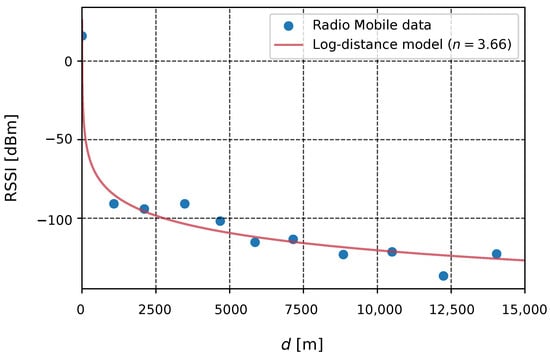
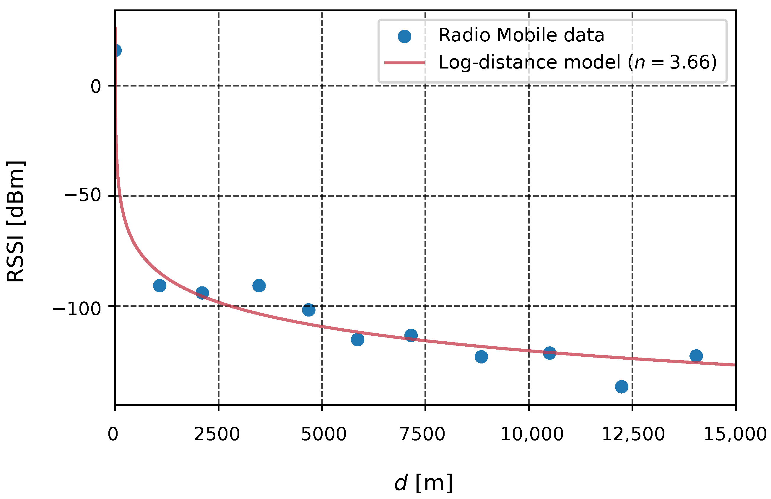
The methods of least squares and the coefficient of determination were used to calculate the best value for n, and to verify the goodness of fit; these are both classic methods of achieving the desired results. In statistics, the coefficient of determination—denoted $R^2$—is the proportion of the variation in the dependent variable that is predictable from the independent variable(s); it is a number between 0 and 1, which measures how well a statistical model predicts an outcome. Figure 5 presents the graph, with the log-distance model and the data collected from the Radio Mobile simulator. The n parameter found was 3.66, and the coefficient of determination for the adjustment was equal to 0.97, for the studied environment.

Figure 5. Received power (dBm) as a function of distance and the log-distance model.

3.4. Simulation Parameters

LoRaWANSim is a free and open-source simulator, developed in MATLAB©, that simulates the behavior of the medium access and physical layer of LoRaWAN; it allows for network designers to evaluate the performance of their networks under different scenarios, including the impact of varying node density, transmission power, and modulation schemes. The simulator is based on a model that allows for the simulation of various network states, including transmission, reception, idle, and low-consumption modes of operation. One limitation of LoRaWANSim is that it does not consider energy consumption in the processing and input/output (I/O) modes, which can be an essential factor in some applications; however, the theoretical model used in this work has the flexibility of making it possible for the network designer to study as many states as needed. Tests and comparisons with analytical models and experimental results were conducted, to validate the simulator. The main inputs of the simulator are the arrangement of the nodes, the propagation model, and a set of parameters that determines the behavior of the protocol stack layers. As outputs, the simulator returns several performance metrics, such as the ULDR (Uplink Data Rate) and the performance of the total and mean energy consumption of each ED [13].

The EDs were placed randomly in a polygonal area determined by the plantation limits. Table 2 contains the list of the parameters used as input to the simulator. Two scenarios were established, to analyze the effects of medium concurrence: Scenario 1 with low-medium concurrence (T = 600 s), and Scenario 2 with high-medium concurrence (T = 60 s). In both scenarios, the number of EDs was 500. Except for the propagation model parameter, the period between transmissions, and the number of GWs and EDs, all other parameters were the same as those in [13].

Table 2. Input parameters for the chosen scenarios.

Parameter	Description	Values
N	Number of nodes	{500}
G	Number of GWs	{$1\dots 20$}
R [km]	Area radius	{9}
$P_T^{ED}$ [dBm]	ED transmission power	{14, 12, 10, 8, 6, 4, 2}
$G_A^{ED}$ [dBi]	ED antenna gain	{5}
$P_T^{GW}$ [dBm]	GW transmission power	{16}
$G_A^{GW}$ [dBi]	ED antenna gain	{5}
$\sigma$ [dB]	Shadowing parameter	{3}
n	Propagation model parameter	{3.66}
$CR$ [bits/s]	Coding rate	{1}
$BW$ [kHz]	Bandwidth	{125}
$DC$ [%]	Duty cycle restriction	{100} (no DC restriction)
T [s]	Period between transmissions	{60, 600}
H [Boolean]	Header Presence?	{1} (true)
$L_p$ [bytes]	Message preamble length	{8}
$B_{UL}$ [bytes]	Uplink packet size	{20}
$B_{DL}$ [bytes]	Downlink packet size	{20}
RX1DROffset	Offset between the SF of transmission and RX1 reception window	{0} (no offset)

3.5. Proposed Method

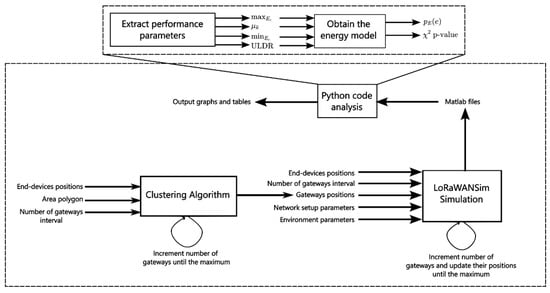
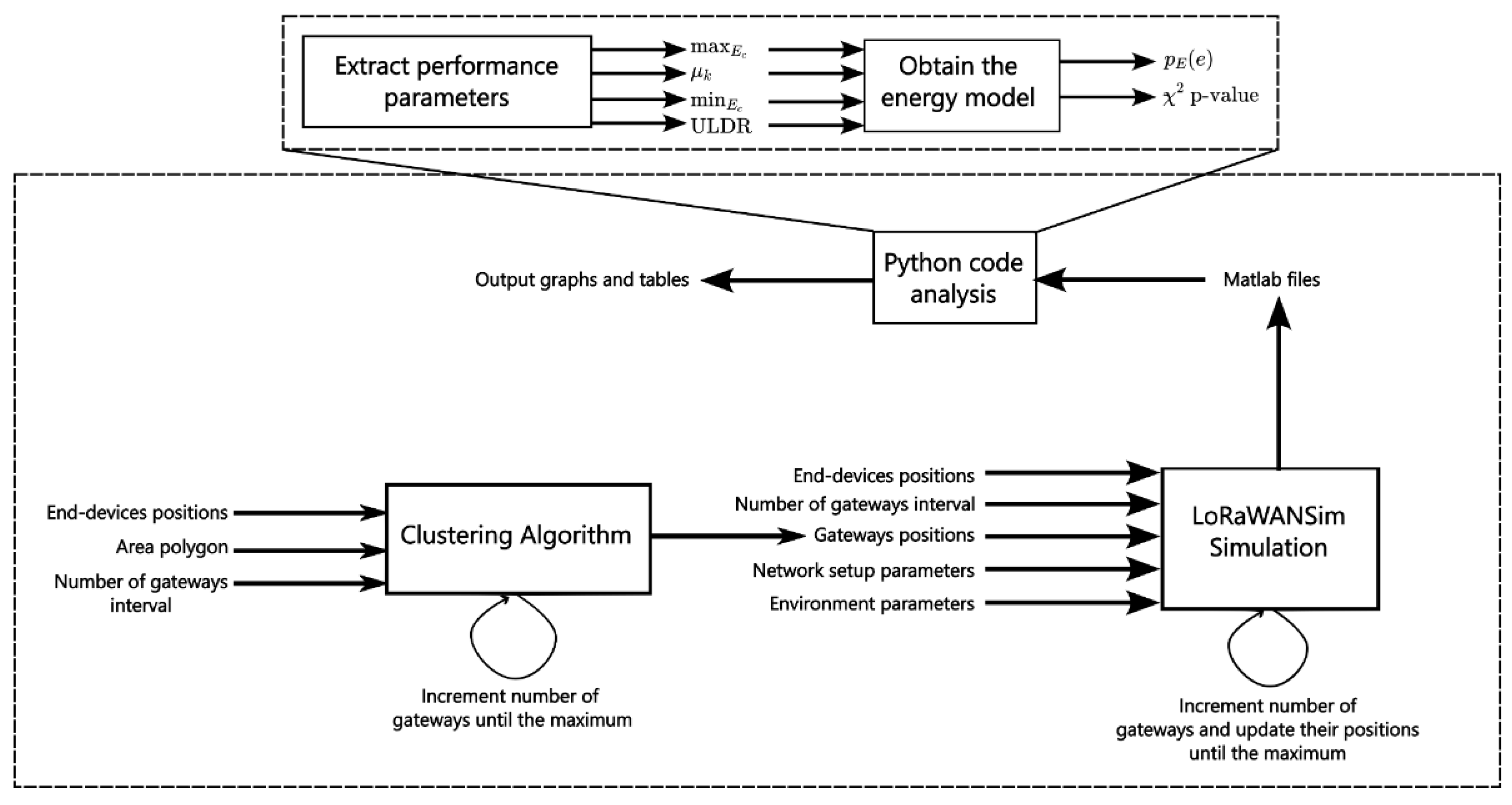
The proposed method for finding the optimal number of GWs, that balances ULDR, energy consumption, and cost, is summarized in Figure 6. The cost was indirectly determined by considering that increasing the number of GWs by one should result in a reasonable ULDR gain or power consumption reduction. The first step was to randomly place the EDs within an established polygon, and to conduct preliminary simulation tests, to find the maximum number of GWs that could achieve a high ULDR. It was found that, for a transmission period of 600 s (with lower-medium concurrence), 10 GWs were sufficient to obtain a high ULDR. For a shorter transmission period of 60 s, 20 GWs were enough. This information was then used as input for the clustering algorithms (K-Means, MiniBatch K-Means, Bisecting K-Means, and FCM), which were executed multiple times, starting with one GW, and increasing the number until the maximum was reached. The goal was to find the number of GWs that improved the ULDR, while fitting the energy consumption to the theoretical energy model.

Figure 6. Diagram of the proposed method to improve and analyze the WSN performance.

The proposed method used the LoRaWANSim simulator to evaluate the performance of a LoRaWAN network under two different scenarios. The simulator was executed with the known different numbers and positions of the GWs, random positions of the EDs, and various radio and environment parameters. The simulator’s output was used to create various Matlab files, which served as input for a Python code developed to generate graphs and tables automatically. The energy consumption per cycle was used to calculate the theoretical PDF curve, which was then compared to the simulation data using the ${\chi }^2$-test. The smallest p-value indicated the best adherence of the model to the data, which implied that the power consumption of the network was close to the minimum, as described in Section 3.2. The objective of the proposed method was to improve energy performance by decreasing the consumption per cycle of all network nodes with a reasonable energy stop criterion, which was accomplished by the ${\chi }^2$-test. As the proposed method was new, the p-value at which the algorithm should stop was unknown, so it was decided to increase the number of GWs to a high amount.

4. Simulation Results and Discussion

This section presents the simulation results regarding the number of GWs suggested by the proposed method, the ULDR, and the energy performance.

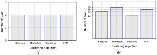
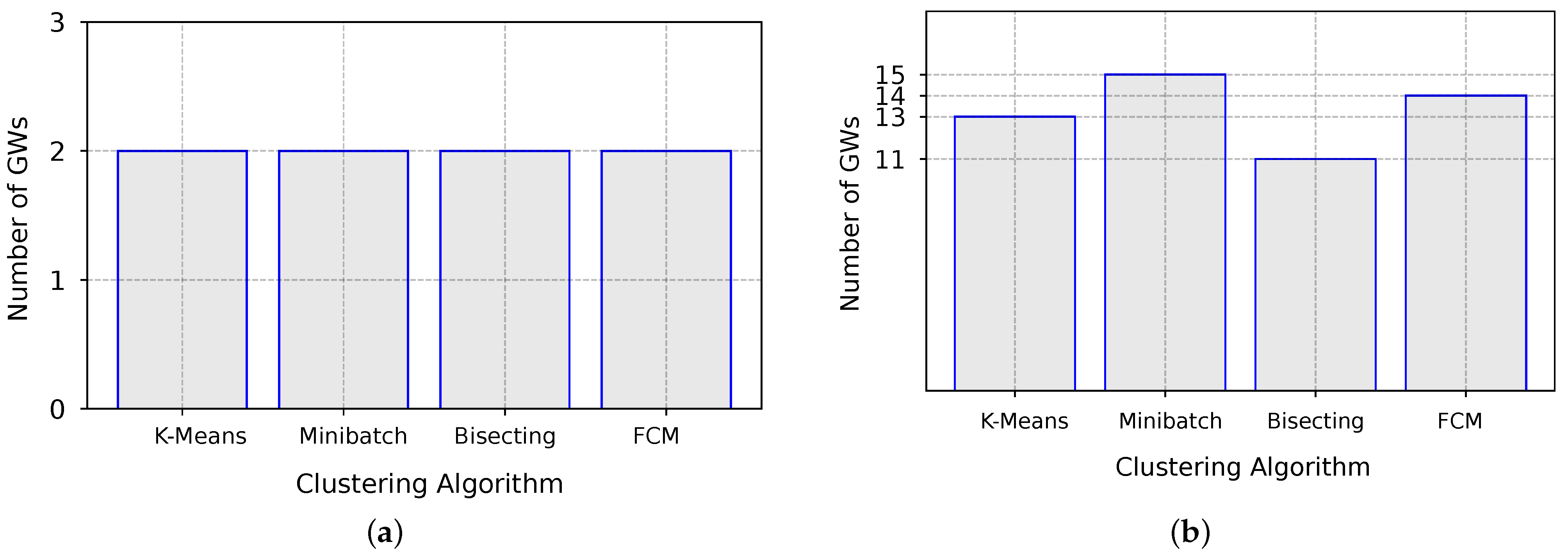
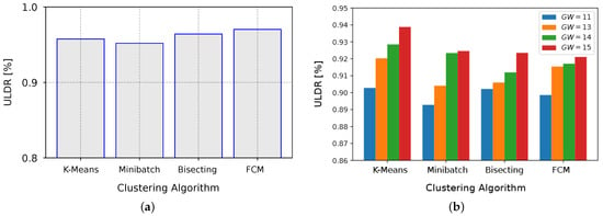
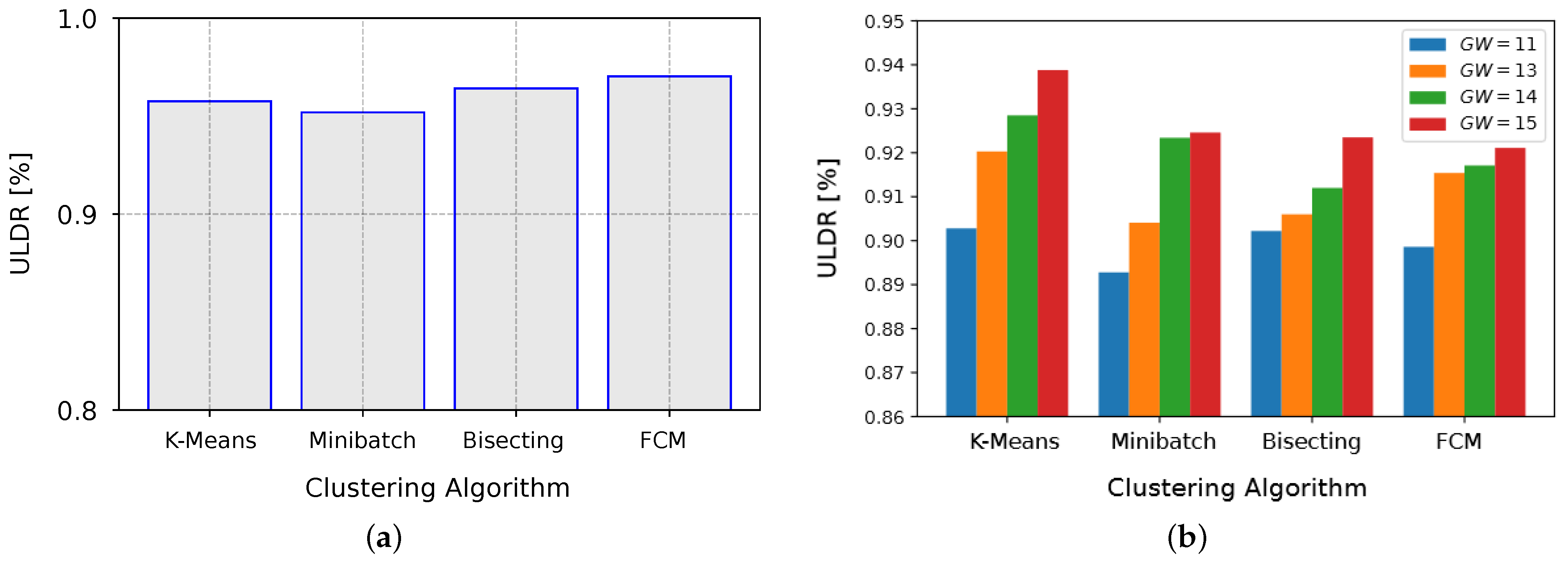
The proposed method used four clustering algorithms (K-Means, Bisecting K-Means, Minibatch K-Means, and FCM) to determine the number of GWs for two different scenarios. Figure 7a illustrates that the suggested method recommended 2 GWs for Scenario 1, based on the results from the four clustering algorithms. For Scenario 2 (Figure 7b), the proposed method suggested a range for the number of GWs that needed to be analyzed in greater detail. The number of GWs at which the minimum p-value occurred was 11, 13, 14, and 15 for K-Means, Bisecting K-Means, Minibatch K-Means, and FCM, respectively. While the energy model may have adhered better with a smaller number of GWs for one algorithm, this did not necessarily mean that its performance, in terms of packet delivery rate and energy usage, was superior to other algorithms that recommend more GWs; therefore, it was essential to compare the metrics for the GW number interval, rather than just evaluating one single metric.

Figure 7. Number of GWs obtained by each clustering algorithm for (a) Scenario 1, and (b) Scenario 2.

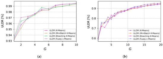
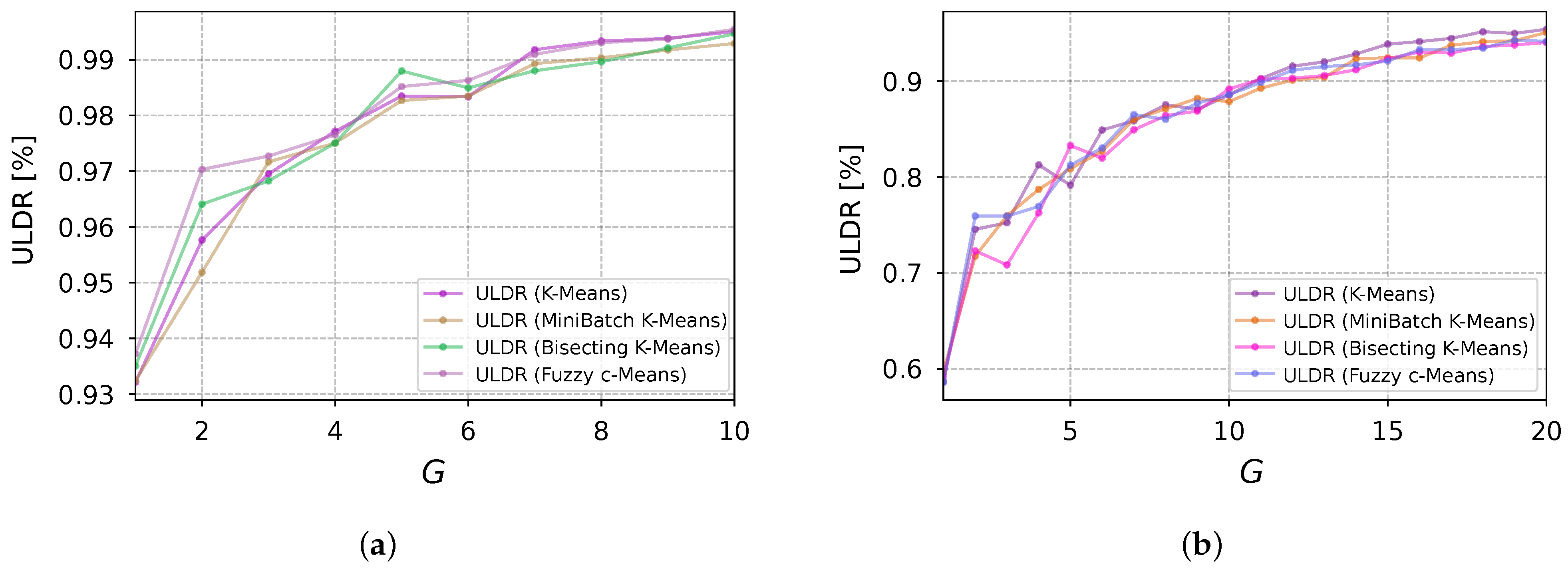
Different cluster models are available in the literature, and distinct algorithms can be provided for each of these cluster models. Clusters discovered by one clustering method will probably differ from clusters discovered by another technique; this explains why the ULDR differed from one algorithm to another in Scenario 2, in which more random factors took place (Figure 8). The performance of the clustering algorithms, regarding the ULDR for Scenario 1, showed no considerable difference among the clustering techniques, according to the graph shown in Figure 8a; the FCM algorithm gave the best performance, by a small margin; on the other hand, considering Scenario 2, Figure 8b shows that the K-Means algorithm performed better for all the suggested GW quantities.

Figure 8. ULDR obtained by the method considering (a) Scenario 1, and (b) Scenario 2.

By analyzing the ULDR values in Figure 9, it can be seen that they improved as the number of GWs increased, for both Scenario 1 and 2; this behavior was expected, as less energy was needed for the EDs to transmit their messages, increasing the SIR (signal-to-interference ratio) and, consequently, reducing packet loss. The Scenario 1 impairment was dominated only by noise, while Scenario 2 impairments were also dominated by collisions and interference. Comparing both scenarios, it can be seen that the ULDR performance improved faster in Scenario 1—that is, with fewer GWs—than in Scenario 2, because of the amount of deterioration signals.

Figure 9. ULDR evolution as a function of the number of GWs obtained by the method considering (a) Scenario 1, and (b) Scenario 2.

Table 3 displays the ULDR values for the lower-medium concurrence case (Scenario 1) when using the clustering techniques. The maximum $\upsilon$ difference was 1.8% for every number of GWs. It can also be seen that the least p-value equaled 0.12 for all clustering algorithms. The average ULDR improvement was 2.67%, when adding the second GW considering all the clustering schemes. From this point forward ($GW>2$), adding more GWs resulted in an average gain of 0.41% per GW added.

Table 3. ULDR and p-values obtained from the application of each clustering method for the different number of GWs (Scenario 1).

GW	${\mathit{\upsilon }}_{\mathit{km}}$	${\mathit{\upsilon }}_{\mathit{mb}}$	${\mathit{\upsilon }}_{\mathit{bk}}$	${\mathit{\upsilon }}_{\mathit{fcm}}$	${\mathit{p}}_{\mathit{km}}$	${\mathit{p}}_{\mathit{mb}}$	${\mathit{p}}_{\mathit{bk}}$	${\mathit{p}}_{\mathit{fcm}}$
1	0.9321	0.9324	0.9351	0.9373	0.2525	0.2663	0.1665	0.2760
2	0.9576	0.9519	0.9641	0.9703	0.1155	0.1180	0.1222	0.1176
3	0.9695	0.9717	0.9683	0.9727	0.1339	0.1618	0.1480	0.1888
4	0.9771	0.9750	0.9750	0.9765	0.1655	0.2414	0.2939	0.2883
5	0.9835	0.9827	0.9880	0.9852	0.2813	0.3236	0.2632	0.3528
6	0.9833	0.9835	0.9849	0.9863	0.2890	0.2654	0.2741	0.2905
7	0.9918	0.9893	0.9880	0.9909	0.5043	0.3351	0.3328	0.2874
8	0.9933	0.9903	0.9896	0.9930	0.6729	0.4268	0.4499	0.2586
9	0.9938	0.9917	0.9921	0.9937	0.7213	0.4789	0.5008	0.3735
10	0.9950	0.9929	0.9946	0.9954	0.4704	1.0000	0.6056	0.9992

The ULDR values for the higher-medium concurrence case (Scenario 2) are shown in Table 4. Differences in the performance are apparent, unlike Scenario 1. For every given total number of GWs, the largest $\upsilon$ difference was 5.13% when GW = 3. The minimum p-value was different for every clustering algorithm. The average ULDR improvement brought about by the addition of 14 GWs (maximum number of GWs) was 33.66%, which gave 2.40% of ULDR gain per added GW, on average. When 5 more GWs were installed, the average gain per added GW was 0.04%.

Table 4. ULDR and p-values obtained from the application of each clustering method for the different number of GWs (Scenario 2).

GW	${\mathit{\upsilon }}_{\mathit{km}}$	${\mathit{\upsilon }}_{\mathit{mb}}$	${\mathit{\upsilon }}_{\mathit{bk}}$	${\mathit{\upsilon }}_{\mathit{fcm}}$	${\mathit{p}}_{\mathit{km}}$	${\mathit{p}}_{\mathit{mb}}$	${\mathit{p}}_{\mathit{bk}}$	${\mathit{p}}_{\mathit{fcm}}$
1	0.5863	0.5970	0.5923	0.5857	0.2076	0.2152	0.2394	0.2450
2	0.7454	0.7174	0.7229	0.7594	0.1054	0.1172	0.1116	0.1268
3	0.7523	0.7596	0.7083	0.7592	0.1079	0.1401	0.1994	0.1180
4	0.8127	0.7871	0.7626	0.7693	0.1162	0.1516	0.1932	0.1394
5	0.7915	0.8087	0.8328	0.8124	0.1607	0.1334	0.1332	0.1189
6	0.8491	0.8270	0.8198	0.8304	0.1228	0.1219	0.1447	0.1575
7	0.8587	0.8602	0.8493	0.8652	0.1223	0.0899	0.1154	0.1037
8	0.8755	0.8712	0.8642	0.8603	0.1019	0.0978	0.0918	0.1070
9	0.8707	0.8821	0.8689	0.8771	0.1114	0.1280	0.1408	0.1390
10	0.8858	0.8787	0.8920	0.8861	0.1237	0.1030	0.1281	0.1174
11	0.9028	0.8928	0.9022	0.8986	0.1028	0.1332	0.0860	0.1157
12	0.9158	0.9012	0.9031	0.9115	0.1320	0.1031	0.1059	0.1181
13	0.9203	0.9041	0.9060	0.9154	0.0709	0.0872	0.1476	0.1014
14	0.9285	0.9234	0.9120	0.9171	0.1045	0.1185	0.1636	0.0927
15	0.9388	0.9246	0.9235	0.9211	0.0901	0.0734	0.1203	0.1446
16	0.9415	0.9244	0.9306	0.9329	0.1377	0.1289	0.1541	0.1248
17	0.9448	0.9376	0.9295	0.9330	0.1410	0.1426	0.1237	0.1659
18	0.9517	0.9413	0.9363	0.9346	0.1149	0.1243	0.1418	0.1106
19	0.9500	0.9424	0.9380	0.9429	0.1503	0.1432	0.1484	0.1493
20	0.9543	0.9509	0.9404	0.9418	0.1185	0.1511	0.1470	0.1339

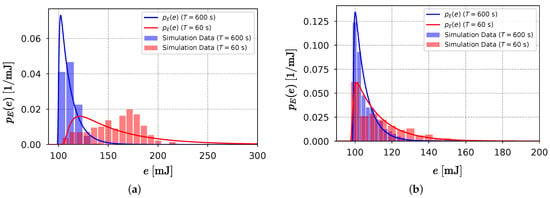
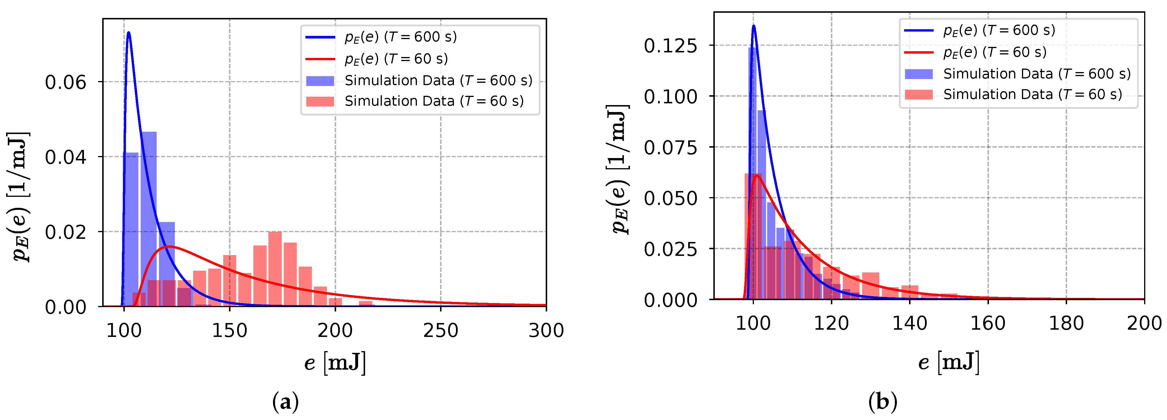
The theoretical model and energy consumption histograms (shown in Figure 10) for the two scenarios are presented before and after the application of the method. Regarding the one GW case (before the method), increasing the time between transmissions decreased power consumption, as expected. For the one GW scenario case, the theoretical PDF was more accurately matched by the simulation findings for T = 600 s. Energy consumption observations for the T = 60 s scenario were outside the expected range for the exponential convolution PDF; this was because of higher interference and collisions, which affected SNR and made the ADR algorithm push the energy values further from the minimum. After the method application, the energy dispersion of both Scenario 1 and 2 closely matched the theoretical energy model. When the number of GWs continued increasing, the energy values became closer to the minimum; however, the ULDR gain and the energy reduction occurred at a much slower rate.

Figure 10. Comparison of the energy performance (a) before and (b) after the proposed method.

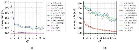
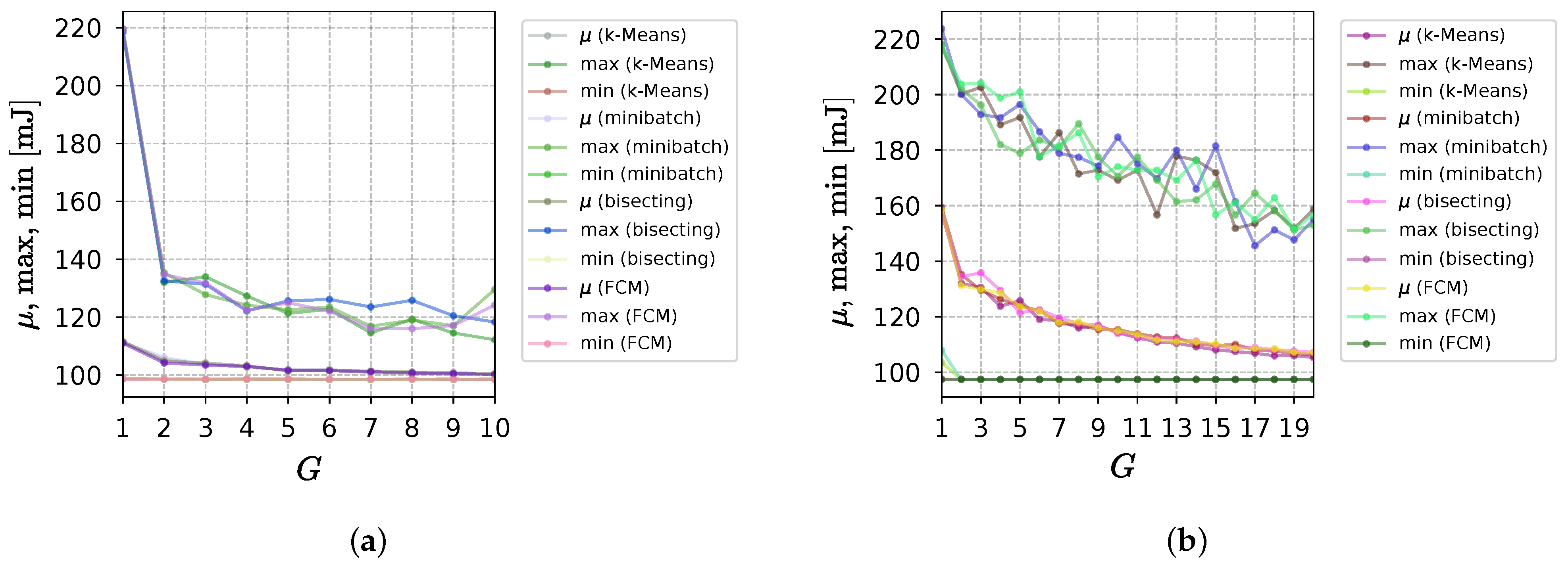
Figure 11 depicts the evolution of maximum, mean, and minimum energy usage over GW amount for Scenarios 1 and 2. Considering the highest energy consumption in Scenario 1, it can be seen that it decreased considerably after the initial increase in the number of GWs. The consumption in Scenario 2, on the other hand, decreased more slowly, and fluctuated more, due to the larger number of factors that disturbed the operation of the network. The application of the method in Scenario 2 saved considerably more energy than Scenario 1, despite the absolute values of power consumption in Scenario 2 remaining higher. The effectiveness of the different clustering techniques was equivalent in both cases. Almost no variation in minimum consumption was observed.

Figure 11. Energy metrics evolution as a function of the number of GWs obtained by the method considering (a) Scenario 1, and (b) Scenario 2.

Table 5 displays the energy values for the lower-medium concurrence case. As the number of GWs increased, the GWs became closer to EDs; this led to SNR increasing, which made the ADR algorithm recommend smaller values of $P_t$ and the SF to the EDs. As a consequence, the mean power consumption decreased. The maximum $\mu$ difference was 1.90 mJ for every number of GWs and clustering algorithms. The average improvement was 6.18 mJ, when adding the second GW, considering all the clustering schemes. From this point forward ($GW>2$), adding more GWs resulted in an average gain of 0.60 mJ per GW added, regarding the mean consumption. As noted above, the minimum consumption hardly ever changed. Great improvement was attained in the maximum consumption. The average saving reduction was 85.58 mJ when adding the second GW. The average improvement for the extra GWs was 1.57 mJ per GW added.

Table 5. Energy metrics for Scenario 1 by algorithm and number of GWs.

GW	${\mathit{\mu }}_{\mathit{km}}$	${\mathit{\mu }}_{\mathit{mb}}$	${\mathit{\mu }}_{\mathit{bk}}$	${\mathit{\mu }}_{\mathit{fcm}}$	${min}_{\mathit{km}}$	${min}_{\mathit{mb}}$	${min}_{\mathit{bk}}$	${min}_{\mathit{fcm}}$	${max}_{\mathit{km}}$	${max}_{\mathit{mb}}$	${max}_{\mathit{bk}}$	${max}_{\mathit{fcm}}$
1	111.43	111.32	111.57	111.06	98.71	98.77	98.77	98.65	219.45	219.59	218.46	219.49
2	105.50	106.11	104.84	104.20	98.59	98.68	98.65	98.57	132.06	135.35	132.57	134.68
3	103.78	103.72	104.16	103.46	98.57	98.54	98.62	98.62	133.97	127.80	131.43	131.82
4	102.75	102.97	103.22	103.02	98.59	98.57	98.57	98.59	127.31	124.17	122.18	122.40
5	101.78	101.86	101.45	101.66	98.59	98.52	98.59	98.59	121.35	122.58	125.64	125.01
6	101.85	101.88	101.66	101.53	98.57	98.54	98.59	98.57	122.75	123.53	126.16	122.07
7	100.85	101.14	101.39	101.15	98.57	98.52	98.57	98.57	114.62	116.89	123.53	116.02
8	100.60	101.00	101.03	100.74	98.57	98.59	98.50	98.59	119.26	119.00	125.84	116.02
9	100.39	100.77	100.76	100.46	98.59	98.52	98.59	98.52	114.54	117.12	120.49	117.13
10	100.11	100.49	100.40	100.28	98.52	98.62	98.57	98.54	112.21	129.60	118.36	124.21

The energy values in the case of a higher-medium concurrence are listed in Table 6. More GWs were required, to provide an acceptable decrease in power usage due to the 10-times increase in medium concurrence. The installation of 14 GWs resulted in an average improvement of 48.71 mJ in the mean energy, and 49.67 mJ in the maximum, or an average of 3.48 mJ and 3.55 mJ reduction in energy consumption per GW for the mean and maximum consumption, respectively. After accounting for the least p-value, the average reduction per additional GW was 2.84 mJ when 5 more GWs were implemented.

Table 6. Energy metrics for Scenario 2 by algorithm and number of GWs.

GW	${\mathit{\mu }}_{\mathit{km}}$	${\mathit{\mu }}_{\mathit{mb}}$	${\mathit{\mu }}_{\mathit{bk}}$	${\mathit{\mu }}_{\mathit{fcm}}$	${min}_{\mathit{km}}$	${min}_{\mathit{mb}}$	${min}_{\mathit{bk}}$	${min}_{\mathit{fcm}}$	${max}_{\mathit{km}}$	${max}_{\mathit{mb}}$	${max}_{\mathit{bk}}$	${max}_{\mathit{fcm}}$
1	157.69	159.32	156.97	158.36	103.53	107.93	97.53	97.48	217.97	223.63	216.92	217.97
2	132.01	135.25	134.48	131.26	97.46	97.47	97.46	97.46	200.25	200.09	202.10	203.72
3	130.54	129.58	135.81	129.87	97.45	97.45	97.45	97.47	202.62	192.81	196.25	204.24
4	123.80	126.36	129.51	128.61	97.46	97.46	97.46	97.46	189.13	191.70	182.01	198.75
5	125.86	123.93	121.44	123.71	97.46	97.46	97.46	97.45	191.79	196.46	178.86	201.05
6	119.08	122.26	122.54	122.04	97.46	97.46	97.46	97.46	177.54	186.58	183.65	177.67
7	118.66	117.59	119.65	117.99	97.44	97.46	97.45	97.45	186.26	178.86	181.02	181.55
8	115.99	117.09	117.52	118.20	97.46	97.46	97.46	97.46	171.46	177.43	189.52	186.26
9	116.65	115.38	117.08	116.03	97.45	97.46	97.45	97.45	172.80	174.24	177.54	170.37
10	114.51	115.37	113.98	114.94	97.45	97.46	97.46	97.44	169.22	184.67	170.58	174.06
11	112.42	113.90	112.65	113.57	97.46	97.46	97.46	97.45	172.80	175.16	177.54	172.80
12	110.95	112.78	112.23	111.60	97.46	97.45	97.46	97.46	156.68	169.80	169.22	172.80
13	110.52	112.35	111.85	111.02	97.45	97.45	97.46	97.46	177.83	179.98	161.44	169.10
14	109.21	110.21	111.23	110.95	97.46	97.46	97.45	97.46	176.39	165.98	162.04	176.39
15	108.10	109.63	109.52	110.25	97.45	97.46	97.45	97.45	171.87	181.49	167.77	156.68
16	107.49	110.04	108.71	108.67	97.45	97.45	97.45	97.45	151.85	161.44	156.66	161.19
17	106.89	108.12	108.97	108.64	97.45	97.45	97.45	97.45	153.53	145.58	164.57	154.96
18	105.96	107.65	108.05	108.47	97.46	97.45	97.46	97.45	158.34	151.29	158.24	162.87
19	106.00	106.84	107.64	107.23	97.45	97.46	97.46	97.46	151.85	147.70	151.29	151.58
20	105.37	106.29	107.27	107.23	97.45	97.46	97.45	97.45	158.73	154.96	152.97	156.66

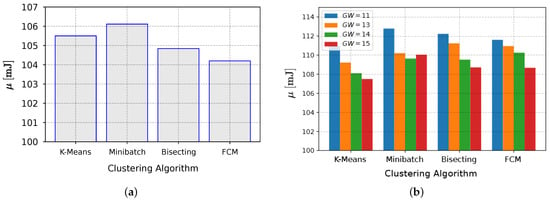
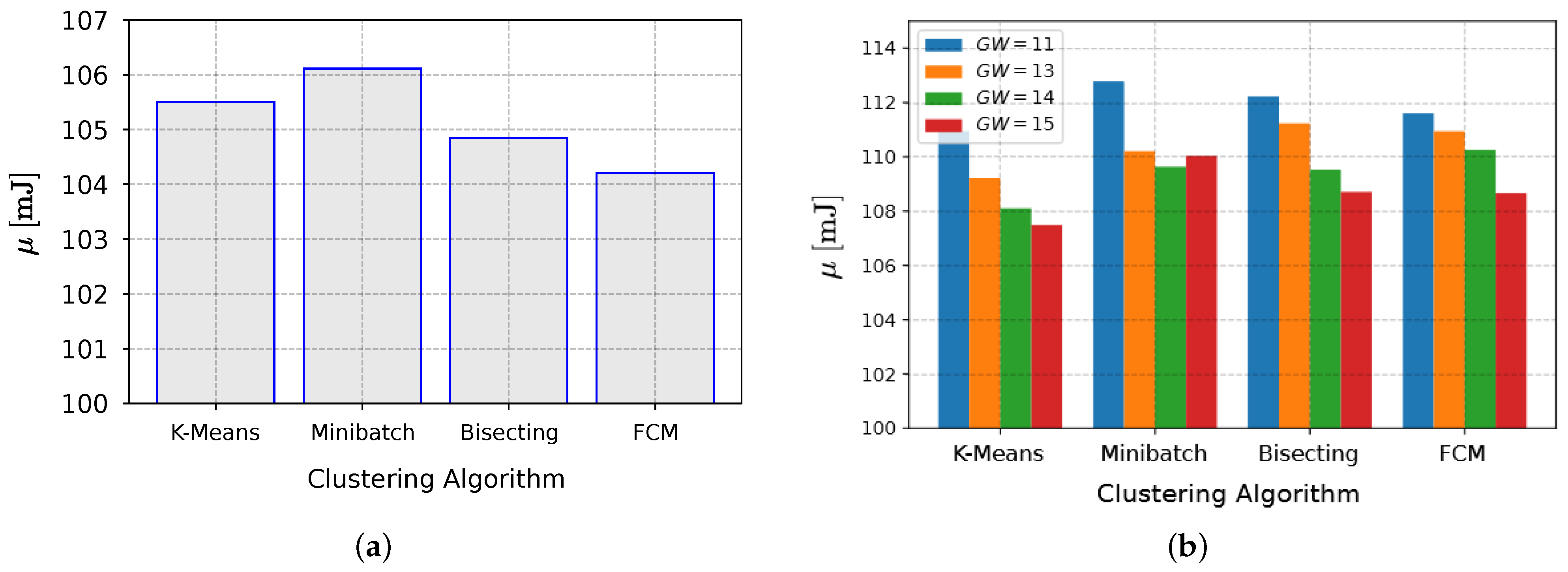
Regarding the lowest p-value results, the mean network energy consumption numbers were relatively close, within a small margin of error, for the setups in Scenario 1; this was in contrast to Scenario 2, in which there was a larger fluctuation in the average consumption of one algorithm compared to the other, as the delivery rate increased. In Scenario 1, the performance of the FCM algorithm was superior, as evidenced by the smallest mean consumption values presented in Figure 12a. Figure 12b presents the findings of Scenario 2, which show that the K-Means technique was superior to the alternatives for all of the GW values.

Figure 12. Mean energy consumption for the best p-value situation considering (a) Scenario 1 (two GWs), and (b) Scenario 2 (GW interval).

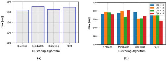
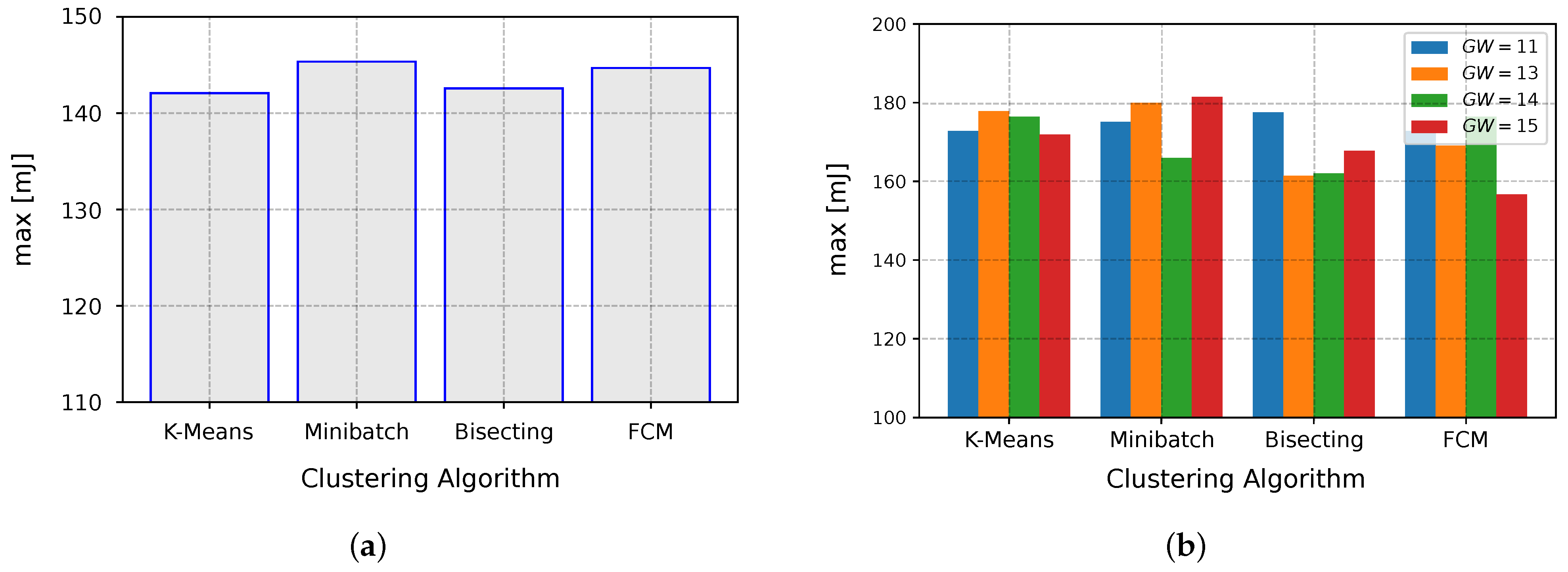
The time at which the network nodes began to run out of power is influenced by the maximum amount of power that they use. For the Scenario 1 settings, the maximum network energy consumption estimates were also very similar, in contrast to Scenario 2, in which the average consumption of one algorithm compared to the other fluctuated more. The K-Means method was more efficient in Scenario 1. Figure 13b illustrates the findings of Scenario 2, which demonstrated that the FCM technique was superior to the alternatives, with 15 GWs.

Figure 13. Maximum energy consumption for the best p-value situation considering (a) Scenario 1 (two GWs), and (b) Scenario 2 (GW interval).

5. Conclusions

This study presents novel and promising outcomes for implementing LoRaWAN in smart agriculture IoT applications in a large agricultural area in one of the most important fruit-producing regions in Brazil. This research offers a comprehensive characterization of the environment, focusing on a real polygonal plantation area. A method for placing LoRaWAN GWs in smart agriculture applications, using K-Means and its variations, is proposed. The use of a stochastic energy model to evaluate power consumption and various performance metrics to support the final deployment decision is also proposed. The authors consider that the main original contribution of this work is the utilization of the stochastic energy model, in conjunction with the clustering algorithms, to solve the GW placement problem for agricultural IoT applications, although the method could be adapted to other technologies and contexts.

Simulations were performed, considering two scenarios that provided insight into the performance of LoRaWAN, showing that the method suggested 2 GWs for Scenario 1 and a range for the number of GWs for Scenario 2. The performance of the clustering algorithms, in terms of the ULDR, was improved after the method application, and varied between the two scenarios and among the different algorithms. The study also found that increasing the time between transmissions decreased power consumption, and that the energy efficiency of the system was improved, reducing the mean and maximum energy consumption. The study concluded that the FCM and K-Means techniques were superior in the different scenarios, with different numbers of GWs for the specific studied parameters.

Future Work

Whether utilizing a particular cluster model or algorithm, the clusters discovered will always be distinct and varied; therefore, the authors intend to study more clustering algorithms, and different network technologies (such as SigFox and NB-IoT) and configurations in the future. It is planned to perform experimental tests in the presented agriculture area.

References

- Kopittke, P.M.; Menzies, N.W.; Wang, P.; McKenna, B.A.; Lombi, E. Soil and the intensification of agriculture for global food security. Environ. Int. 2019, 132, 105078. [Google Scholar] [CrossRef] [Scilit] [PubMed]
- Javaid, M.; Haleem, A.; Singh, R.P.; Suman, R. Enhancing smart farming through the applications of Agriculture 4.0 technologies. Int. J. Intell. Netw. 2022, 3, 150–164. [Google Scholar] [CrossRef] [Scilit]
- Sendra, S.; Parra, L.; Jimenez, J.M.; Garcia, L.; Lloret, J. LoRa-based network for water quality monitoring in coastal areas. Mob. Netw. Appl. 2022, 1–17. [Google Scholar] [CrossRef] [Scilit]
- Malik, P.K.; Sharma, R.; Singh, R.; Gehlot, A.; Satapathy, S.C.; Alnumay, W.S.; Pelusi, D.; Ghosh, U.; Nayak, J. Industrial Internet of Things and its applications in industry 4.0: State of the art. Comput. Commun. 2021, 166, 125–139. [Google Scholar] [CrossRef] [Scilit]
- Coman, F.L.; Malarski, K.M.; Petersen, M.N.; Ruepp, S. Security issues in internet of things: Vulnerability analysis of LoRaWAN, sigfox and NB-IoT. In Proceedings of the IEEE 2019 Global IoT Summit (GIoTS), Aarhus, Denmark, 17–21 June 2019; pp. 1–6. [Google Scholar]
- Almuhaya, M.A.; Jabbar, W.A.; Sulaiman, N.; Abdulmalek, S. A survey on Lorawan technology: Recent trends, opportunities, simulation tools and future directions. Electronics 2022, 11, 164. [Google Scholar] [CrossRef] [Scilit]
- Abbasi, M.; Khorasanian, S.; Yaghmaee, M.H. Low-power wide area network (lpwan) for smart grid: An in-depth study on Lorawan. In Proceedings of the IEEE 2019 5th Conference on Knowledge Based Engineering and Innovation (KBEI), Tehran, India, 28 February–1 March 2019; pp. 22–29. [Google Scholar]
- Medeiros, D.d.F.; Souza, C.P.d.; Carvalho, F.B.S.; Lopes, W.T.A. Energy-Saving Routing Protocols for Smart Cities. Energies 2022, 15, 7382. [Google Scholar] [CrossRef] [Scilit]
- Sadeeq, M.A.; Zeebaree, S. Energy management for internet of things via distributed systems. J. Appl. Sci. Technol. Trends 2021, 2, 59–71. [Google Scholar] [CrossRef] [Scilit]
- Shahraki, A.; Taherkordi, A.; Haugen, Ø.; Eliassen, F. Clustering objectives in wireless sensor networks: A survey and research direction analysis. Comput. Netw. 2020, 180, 107376. [Google Scholar] [CrossRef] [Scilit]
- Hassan, A.A.h.; Shah, W.M.; Othman, M.F.I.; Hassan, H.A.H. Evaluate the performance of K-Means and the fuzzy C-Means algorithms to formation balanced clusters in wireless sensor networks. Int. J. Electr. Comput. Eng. 2020, 10, 1515–1523. [Google Scholar] [CrossRef] [Scilit]
- Chen, J.; Wosinska, L.; Machuca, C.M.; Jaeger, M. Cost vs. reliability performance study of fiber access network architectures. IEEE Commun. Mag. 2010, 48, 56–65. [Google Scholar] [CrossRef] [Scilit]
- Marini, R.; Mikhaylov, K.; Pasolini, G.; Buratti, C. LoRaWanSim: A flexible simulator for LoRaWAN networks. Sensors 2021, 21, 695. [Google Scholar] [CrossRef] [Scilit] [PubMed]
- Augustin, A.; Yi, J.; Clausen, T.; Townsley, W.M. A study of LoRa: Long range & low power networks for the internet of things. Sensors 2016, 16, 1466. [Google Scholar] [PubMed]
- de Carvalho Silva, J.; Rodrigues, J.J.; Alberti, A.M.; Solic, P.; Aquino, A.L. LoRaWAN—A low power WAN protocol for Internet of Things: A review and opportunities. In Proceedings of the IEEE 2017 2nd International Multidisciplinary Conference on Computer and Energy Science (SpliTech), Split, Croatia, 12–14 July 2017; pp. 1–6. [Google Scholar]
- Zhou, Q.; Zheng, K.; Hou, L.; Xing, J.; Xu, R. Design and implementation of open LoRa for IoT. IEEE Access 2019, 7, 100649–100657. [Google Scholar] [CrossRef] [Scilit]
- San Cheong, P.; Bergs, J.; Hawinkel, C.; Famaey, J. Comparison of LoRaWAN classes and their power consumption. In Proceedings of the 2017 IEEE Symposium on Communications and Vehicular Technology (SCVT), Leuven, Belgium, 14 November 2017; pp. 1–6. [Google Scholar]
- Elbsir, H.E.; Kassab, M.; Bhiri, S.; Bedoui, M.H. Evaluation of LoRaWAN class B performances and its optimization for better support of actuators. Comput. Commun. 2023, 198, 128–139. [Google Scholar] [CrossRef] [Scilit]
- Kufakunesu, R.; Hancke, G.P.; Abu-Mahfouz, A.M. A survey on adaptive data rate optimization in lorawan: Recent solutions and major challenges. Sensors 2020, 20, 5044. [Google Scholar] [CrossRef] [Scilit]
- Rokach, L.; Maimon, O. Clustering methods. In Data Mining and Knowledge Discovery Handbook; Springer: Berlin/Heidelberg, Germany, 2005; pp. 321–352. [Google Scholar]
- Ikotun, A.M.; Ezugwu, A.E.; Abualigah, L.; Abuhaija, B.; Heming, J. K-means Clustering Algorithms: A Comprehensive Review, Variants Analysis, and Advances in the Era of Big Data. Inf. Sci. 2022, 622, 139. [Google Scholar] [CrossRef] [Scilit]
- Pickens, A.; Sengupta, S. Benchmarking studies aimed at clustering and classification tasks using K-means, fuzzy C-means and evolutionary neural networks. Mach. Learn. Knowl. Extr. 2021, 3, 695–719. [Google Scholar] [CrossRef] [Scilit]
- Feltrin, L.; Buratti, C.; Vinciarelli, E.; De Bonis, R.; Verdone, R. LoRaWAN: Evaluation of link-and system-level performance. IEEE Internet Things J. 2018, 5, 2249–2258. [Google Scholar] [CrossRef] [Scilit]
- Miles, B.; Bourennane, E.B.; Boucherkha, S.; Chikhi, S. A study of LoRaWAN protocol performance for IoT applications in smart agriculture. Comput. Commun. 2020, 164, 148–157. [Google Scholar] [CrossRef] [Scilit]
- Kamonkusonman, K.; Phunthawornwong, M.; Tempiem, P.; Silapunt, R. Utilization-Weighted Algorithm for LoRaWAN Capacity Improvement for Local Smart Dairy Farms in Ratchaburi Province of Thailand. IEEE Access 2021, 9, 141738–141746. [Google Scholar] [CrossRef] [Scilit]
- de Medeiros, E.L.; de Carvalho, F.B.S.; Villanueva, J.M.M.; de Moreira, C.S.; Souza Filho, C.A.d. Data Acquisition System Using Hybrid Network Based on LoRa for Hydraulic Plants. IEEE Trans. Instrum. Meas. 2021, 70, 1–12. [Google Scholar] [CrossRef] [Scilit]
- Yascaribay, G.; Huerta, M.; Silva, M.; Clotet, R. Performance Evaluation of Communication Systems Used for Internet of Things in Agriculture. Agriculture 2022, 12, 786. [Google Scholar] [CrossRef] [Scilit]
- Singh, R.K.; Rahmani, M.H.; Weyn, M.; Berkvens, R. Joint Communication and Sensing: A Proof of Concept and Datasets for Greenhouse Monitoring Using LoRaWAN. Sensors 2022, 22, 1326. [Google Scholar] [CrossRef] [Scilit] [PubMed]
- Rady, M.; Hafeez, M.; Zaidi, S.A.R. Computational methods for network-aware and network-agnostic IoT low power wide area networks (LPWANs). IEEE Internet Things J. 2019, 6, 5732–5744. [Google Scholar] [CrossRef] [Scilit]
- Alenezi, M.; Chai, K.K.; Alam, A.S.; Chen, Y.; Jimaa, S. Unsupervised learning clustering and dynamic transmission scheduling for efficient dense LoRaWAN networks. IEEE Access 2020, 8, 191495–191509. [Google Scholar] [CrossRef] [Scilit]
- Matni, N.; Moraes, J.; Oliveira, H.; Rosário, D.; Cerqueira, E. LoRaWAN gateway placement model for dynamic Internet of Things scenarios. Sensors 2020, 20, 4336. [Google Scholar] [CrossRef] [Scilit]
- Mendes, B.; Correia, N.; Passos, D. On the Optimization of LoRaWAN Gateway Placement in Wide Area Monitoring Systems. In Proceedings of the IFIP International Internet of Things Conference, Amsterdam, The Netherlands, 27–28 October 2022; pp. 41–51. [Google Scholar]
- Cruz, H.A.; Ferreira, S.C.; Araújo, J.P.; Barros, F.J.; Farias, F.S.; Neto, M.C.; Tostes, M.E.; Nascimento, A.A.; Cavalcante, G.P. Methodology for LoRa Gateway Placement Based on Bio-Inspired Algorithmsfor a Smart Campus in Wooded Area. Sensors 2022, 22, 6492. [Google Scholar] [CrossRef] [Scilit]
- Correia, F.; Alencar, M.; Assis, K. Stochastic Modeling and Analysis of the Energy Consumption of Wireless Sensor Networks. IEEE Lat. Am. Trans. 2023, 100, 672494. [Google Scholar]
- Corporation, S. LoRaWAN–Simple Rate Adaptation Recommended Algorithm. Semtech. 2016. Available online: https://www.thethingsnetwork.org/forum/uploads/default/original/2X/7/7480e044aa93a54a910dab8f0adfb5f515d14a1.pdf (accessed on 13 September 2020).
- YAMASHITA, A.; HATA, T. Sustainability of Irrigation Fruit Farming in Terms of Water Supply-demand Situation: Case Study of the Middle Basin of São Francisco River, Northeast Brazil. Geogr. Rev. Jpn. Ser. B 2021, 94, 1–17. [Google Scholar]
- El Khaled, Z.; Ajib, W.; Mcheick, H. Log Distance Path Loss Model: Application and Improvement for Sub 5 GHz Rural Fixed Wireless Networks. IEEE Access 2022, 10, 52020–52029. [Google Scholar] [CrossRef] [Scilit]
- Cordero, L.S.; Adasme, P. Simulating Radio Coverage with polar Coordinates for Wireless Networks. In Proceedings of the IEEE 2021 Third South American Colloquium on Visible Light Communications (SACVLC), Toledo, Brazil, 11–12 November 2021; pp. 01–06. [Google Scholar]
Disclaimer/Publisher’s Note: The statements, opinions and data contained in all publications are solely those of the individual author(s) and contributor(s) and not of MDPI and/or the editor(s). MDPI and/or the editor(s) disclaim responsibility for any injury to people or property resulting from any ideas, methods, instructions or products referred to in the content. |
© 2023 by the authors. Licensee MDPI, Basel, Switzerland. This article is an open access article distributed under the terms and conditions of the Creative Commons Attribution (CC BY) license (https://creativecommons.org/licenses/by/4.0/).