Using MPC to Balance Intermittent Wind and Solar Power with Hydro Power in Microgrids

Abstract

In a microgrid connected with both intermittent and dispatchable sources, intermittency caused by sources such as solar and wind power plants can be balanced by dispatching hydro power into the grid. Both intermittent generation and consumption are stochastic in nature, not known perfectly, and require future prediction. The stochastic generation and consumption will cause the grid frequency to drift away from a required range. To improve performance, operation should be optimized over some horizon, with the added problem that intermittent power varies randomly into the future. Optimal management of dynamic system over a future horizon with disturbances is often posed as a Model Predictive Control (MPC) problem. In this paper, we have employed an MPC scheme for generating a hydro-turbine valve signal for dispatching necessary hydro power to the intermittent grid and maintaining grid frequency. Parameter sensitivity analysis shows that grid frequency is mostly sensitive to the turbine valve signal. We have found that controller discretization time, grid frequency, and power injection into the grid are interrelated, and play an important role in maintaining the grid frequency within the thresholds. Results also indicate that the fluctuations in grid frequency are insignificant on the turbine valve position during power injection into the grid.

1. Introduction

1.1. Background

Electricity generation from renewable energy has increased because of the rise in coal prices, oil insecurity, climatic concern, and the nuclear power debate. There is a demand for a renewable-sources economy over the coal-fired economy. Renewable energy sources are a combination of intermittent and dispatchable energy sources. Intermittent sources such as solar, wind, and tidal power plants exhibit fluctuating power production that creates an imbalance between generation and load. Renewable dispatchable sources such as hydro power plants play a significant role in balancing out the variability caused by intermittent sources. In a microgrid consisting of solar power and wind power supplied with a dispatchable hydro power plant, injection of intermittent solar and wind power creates a fluctuation in grid frequency. The grid frequency must be maintained at the range of $\left(314\pm 5\%\right)\mathrm{rad}/\mathrm{s}$. Furthermore, grid voltage at all levels of generation, transmission, and distribution should also be maintained within the required range. In this regard, it is of interest to dispatch the required hydro power into the grid for balancing intermittent generation and load to maintain grid frequency and voltage level in a microgrid supplied by solar and wind power within the required ranges.

Prospective scenarios on balancing large-scale grid integrated intermittent generations from Northern Europe are outlined with key findings in [1] using Norwegian hydro powers. Reservoirs in Norway are considered to be rechargeable batteries with integration with intermittent generations supplying excess power for pumping water into an upper reservoir from a lower reservoir [2]. The finding indicates that reservoir productions in Norway should be doubled to address the variability of intermittent generations in Northern Europe. The concept of flexible hydro power is coined in [3] indicating cascaded hydro power plants as an example. Current state-of-the-art regarding use of Norwegian hydro power for balancing solar and wind power variability in Continental Europe is reviewed in [4] indicating extensive research on modeling future variability. These studies in the variability of solar and wind power indicate the need for flexible hydro power that can dispatch necessary power by running the synchronous machine in either generator mode or motor mode, where motor mode involves using the machine to pump water back into the reservoir. However, there exist major technical challenges regarding the integration of intermittent energy sources into the grid. One of the major issues is grid frequency stability. A brief technical review of challenges of grid integration of solar and wind power is explored in [5]. A more comprehensive review regarding the challenges in wind power integration into the grid is given in [6]. From the outcomes of preliminary research surveys and discussions, grid frequency fluctuation is the major challenge of grid integration of intermittent generation.

A perfect balance between intermittent generation and consumption can only be achieved if intermittent production is known perfectly, consumption is known perfectly, and hydro power production can be changed infinitely fast. In reality, changes in hydro power production are constrained by inertia in water and rotating mass, and the need to avoid wear and tear in actuators and other equipment. Unknown consumption leads to power imbalance which eventually is observed in a drift in grid frequency. Improved performance requires the operation of the system optimized over some horizon with the added problem that intermittent power varies randomly into the future. Optimal management of dynamic systems over a future horizon with disturbances is often posed as an MPC problem. In this regard, it is of interest to use MPC to balance intermittent generation and consumption by controlling the hydro-turbine valve signal. The problem of grid frequency fluctuation motivates for studying dynamic models of components in an interconnected grid which requires a multiphysics simulation environment. To address more realistic grid fluctuations in a real-time interconnected grid requires a dynamic model of hydro power systems, dynamic model solar power systems, dynamic model of wind energy conversion systems, electrical systems, generation, transmission, and distribution systems including end-users of electricity. This adheres to the choice of the multiphysics simulation environment.

1.2. Previous Studies

A non-linear MPC for controlling hydro-turbine valve signal is presented in [7]. Similarly, a coordinated and robust distributed MPC strategy is studied in [8,9], respectively, for load frequency control. A basic strategy on using MPC for hydro power systems is presented in [10] with emphasis on mathematical models of hydro power systems. A clearer understanding of MPC controllers for large-scale hydro power production is presented formulating a linear dynamical system in [11]. A similar approach for grid frequency control in an interconnected Egyptian grid with renewable powers is explained and studied in [12] using MATLAB. The simulation results with different operating conditions and disturbances from the paper emphasize the use of an MPC-based approach over the optimal Proportional and Integral (PI) controllers. Furthermore, the choice of MPCs over PI controllers with robust handling of disturbances are explained in [13,14,15]. Overall speculations on previous studies emphasize the use of an MPC for controlling hydro-turbine valve signal over a conventional controlling scheme.

1.3. Assumptions and Limitation

The overall system consists of a dynamic model of hydropower system and a steady-state model of a synchronous generator, solar power plant, wind power plant, and consumer load. The dynamics of grid frequency is captured using the swing equation. The detailed assumptions are made throughout the paper when necessary. The angular grid frequency $\omega$ is measured in rad/s, and grid frequency f is measured in Hz, and are related as $\omega =2\pi f$. Since we considered a steady-state model of the synchronous generator and a dynamical model of the hydro-turbine system, we adhere to represent the frequency of rotational dynamical hydro-turbine with angular frequency. As the angular frequency of the hydro-turbine is the same as the angular frequency of the grid for the system we are studying, thus, throughout the paper grid frequency will particularly represent angular grid frequency.

The problem of maintaining the voltage at all levels of generation, transmission, and distribution is out of the scope of this paper.

1.4. Outline and Contributions

A system description of our microgrid is given in Section 2. Section 3 provides mathematical model development. Section 4 address open-loop analysis for parameter sensitivity analysis. The implementation of the MPC is explained in Section 5. Section 6 provides results and discussions with conclusions presented in Section 7. The paper ends with providing suggestions for future work.

Readers are requested to follow figures while reading the results and discussions section. This way, the readers find the information presented in the paper in a lucid way.

Following are the original research contributions from the paper:

(1)

finding controller discretization time constraining the grid frequency, maintained at the required range, based on the rate of change of intermittent generation

(2)

a daily prediction of solar power, and consumer load using relaxation parameters for the Weibull and normal distributions

(3)

a yearly average hydro scheduling for balancing load and generation using yearly parameter spaces for Weibull and normal distributions.

A conceptual framework for finding discretization time for the controller is explained in Section 4. Similarly, Section 5.2 provides a conceptual framework for the daily prediction of solar power, daily prediction of consumer load, and yearly hydro schedule.

2. System Description

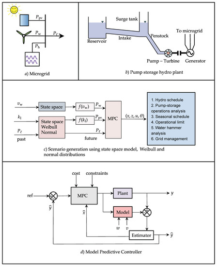
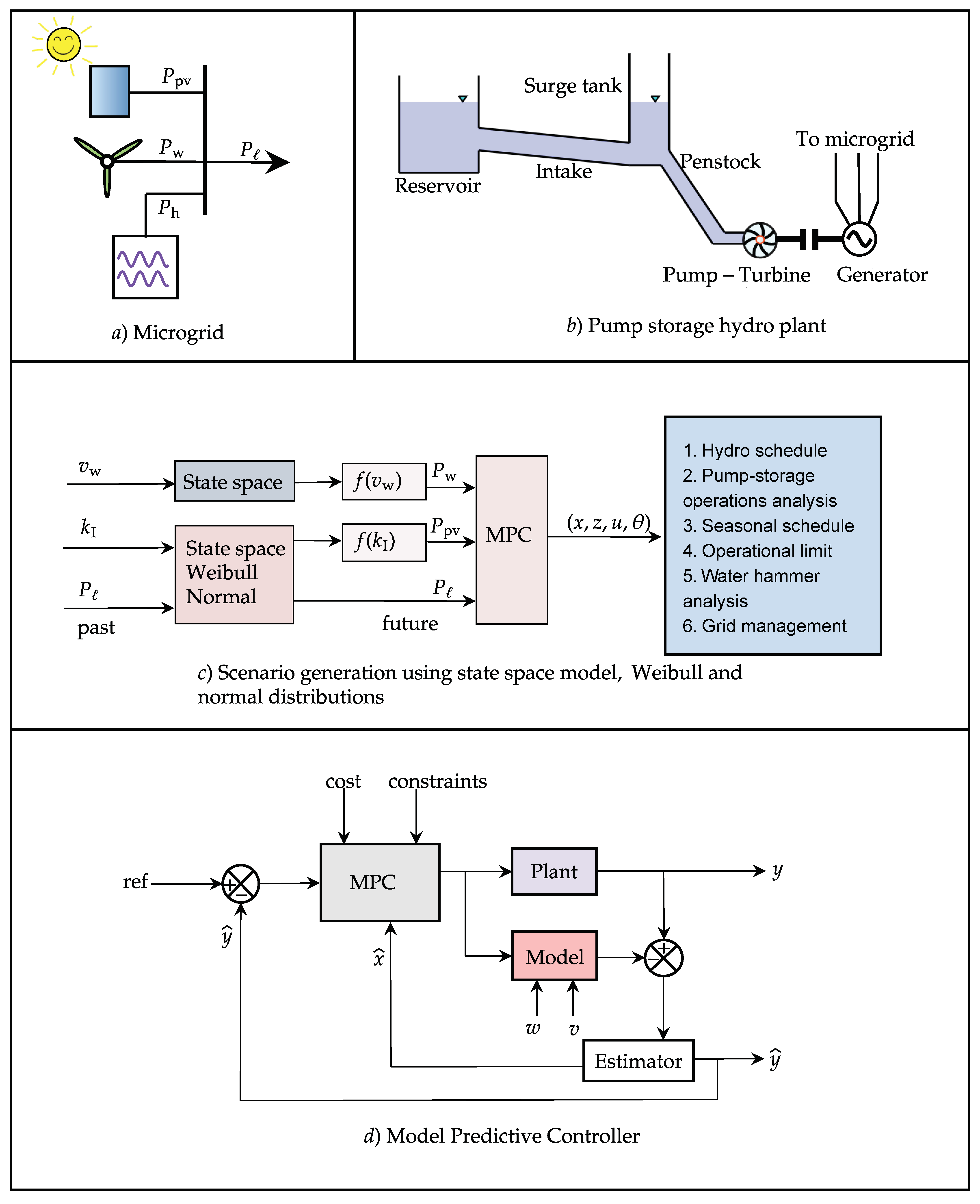
Figure 1a shows a microgrid supplying load power $P_{\ell }$ with intermittent generations from solar and wind energy with power as $P_{\mathrm{pv}}$ and $P_{\mathrm{w}}$, respectively, and a dispatchable hydropower $P_{\mathrm{h}}$. When the intermittent generation is higher than the scheduled load, the hydro power plant is operated in pumping = motoring mode while operated as turbine = generating mode when intermittent generations are insufficient to supply the load. Without considering a dynamical model of the microgrid the needed hydro power for balancing intermittent generation and load is given as,

$$\begin{array}{c}\hfill P_{\mathrm{h}}=P_{\ell }-P_{\mathrm{pv}}-P_{\mathrm{w}}.\end{array}$$

(1)

Figure 1. System block diagram.

Equation (1) is naive and unrealistic; such an approach will not work in a real dynamical system for several reasons. In principle, a hydro-turbine valve cannot be changed instantaneously because of the inertial effect of hydro power plant. Even if it were possible to make instantaneous changes in the hydro-turbine valve, this would lead to excessive water hammer effects, with resulting wear and tear of the equipment. In addition, intermittent generation and scheduled load is not measured directly, and are uncertain. Hence, the imbalance is inferred indirectly through a variation in the grid frequency $\omega$. The grid frequency is a response of the dynamic system given by the combined dynamics of power production and the swing equation as described in Section 3.

Figure 1b shows a hydro-electric plant that can be operated as pump-storage plant. The pump-turbine is coupled with a synchronous machine supplying power to the microgrid. The electrical synchronous machine works as a synchronous motor when hydro power is operated in motoring mode. The hydropower plant consists of a reservoir, intake, surge tank, penstock, and the pump-turbine mechanically coupled with a rotating shaft of the synchronous machine. The number of units of pump-turbine and its power rating can be different based on solar irradiance, wind velocity, and consumer load at different locations. A power system planning engineer should usually select the rating of each of the pump-turbine unit based on the location. For simplicity, we choose a case study discussed in Section 3.4 with 4 units of pump-turbines rated with $1.5\mathrm{MW}$ each. For simplicity, procedures for calculating the ratings are considered to be out of the scope of this paper. However, we will explain the choice of rating in Section 6.

Stochastic scenarios for the wind velocity, solar irradiance, and consumer load demand can be generated from a state-space model as shown in Figure 1c. The solar irradiance scenarios can be generated using confined space (The spaces of Weibull and normal distributions are infinite. The infinite spaces are then converted into a day confined or limited to 24 h. That way a daily solar irradiance is predicted.) for 24 h for Weibull and normal distribution which is presented in Section 5. The future scenarios are generated using past measurement data. Based on the future scenarios for wind velocity and solar irradiance, we calculate solar and wind power. The generated scenarios for wind power, solar power, and consumer load then feed into MPC for computing controlled states, algebraic variables, inputs, and statistical moments. The computed variables from the scenarios are then further analyzed for optimal scheduling of hydro power to be dispatched into the grid. The computed variables also provide information about the operating range of hydro power, pump-turbine operation cycles, seasonal hydro schedule, the operational limit of units, water hammer analysis for hydro units, and information on the microgrid management under stochastic solar and wind power input.

Figure 1d shows a block diagram of MPC with an estimator. We are using an Unscented Kalman filter (UKF) for estimation of states. v and w are process disturbance and measurement noise, respectively. The best estimated states $\widehat{x}$ from the estimator is used for initializing model constraints inside the MPC formulation. y and $\widehat{y}$ are measurement and estimated outputs, respectively.

3. Mathematical Model

3.1. Hydro-Turbine System

The model of hydropower system is based on mass and momentum balance as given by Equations (2) and (3) as,

$$\begin{array}{cc}\hfill \frac{dm}{dt}& =\dot{m}\hfill \end{array}$$

(2)

$$\begin{array}{cc}\hfill \frac{d\mathcal{M}}{dt}& =\dot{\mathcal{M}}+F,\hfill \end{array}$$

(3)

where m is the mass of water, $\dot{m}={\dot{m}}_{\mathrm{i}}-{\dot{m}}_{\mathrm{e}}$ is the difference between influent and effluent mass flow rates, $\mathcal{M}$ is the momentum, $\dot{\mathcal{M}}={\dot{\mathcal{M}}}_{\mathrm{i}}-{\dot{\mathcal{M}}}_{\mathrm{e}}$ is the difference between influent and effluent momentum flow rates, and F is the total force acting on the system. Furthermore, we consider in-compressible water and inelastic pipes. The effect of water temperature is not considered while modeling the system.

For a general pipe unit with influent and effluent pressures as $p_{\mathrm{i}}$ and $p_{\mathrm{e}}$, cross-sectional area A, length L and height difference H, Equations (2) and (3) can be further developed with series of algebraic equations as, $\dot{m}=0$, $\mathcal{M}=mv=\rho AL\frac{\dot{V}}{A}=\rho L\dot{V}$, $\dot{\mathcal{M}}=\dot{m}v=0$, $F=F_p-F_r-F_g$ where $F_p=\left(p_i-p_e\right)A$, $F_g=mg\frac{H}{L}$ and $F_r=\rho L\frac{\pi D\dot{V}\mid \dot{V}\mid }{8A^2}{f}_D$, where v is the velocity of water inside the pipe, $\rho$ is the density of water, $F_{\mathrm{p}}$ is the force due to water pressure, $F_{\mathrm{r}}$ is the fluid frictional force, and $F_{\mathrm{g}}$ is the force under acceleration due to gravity g.

The dynamic equation for volumetric flow rate $\dot{V}$ is then written as,

$$\frac{d\dot{V}}{dt}=\frac{A}{\rho L}\left(p_i-p_e\right)-gA\frac{H}{L}-\frac{\pi D\dot{V}\mid \dot{V}\mid }{8A^2}{f}_D,$$

where Darcy friction factor $f_D$ is calculated based on Reynolds number $N_{\mathrm{Re}}=\frac{\rho \mid v\mid D}{\mu }=\frac{4\rho \mid \dot{V}\mid }{\mu \pi D}$ as,

$$f_D=\left\{\begin{array}{cc}\frac{64}{N_{\mathrm{Re}}}\hfill & N_{\mathrm{Re}}<2100\hfill \\ \frac{1}{{\left(2{log}_{10}\left(\frac{\epsilon }{3.7D}+\frac{5.7}{N_{\mathrm{Re}}^{0.9}}\right)\right)}^2}\hfill & N_{\mathrm{Re}}>2300\hfill \end{array}\right..$$

Here, $\mu$ is the kinematic viscosity of water and $\epsilon$ is the pipe roughness height. For the region with $2100\le N_{\mathrm{Re}}\le 2300$, $f_{\mathrm{D}}$ is calculated by using cubic interpolation, with coefficients differentiable at the boundaries.

For the system shown in Figure 1b, the dynamic equations of hydropower with intake, surge tank and penstock, subscripted with $\mathrm{i}$, $\mathrm{s}$ and $\mathrm{p}$ for e.g., ${\dot{V}}_{\mathrm{s}}$, can be written as,

$$\begin{array}{cc}\hfill \frac{dh}{dt}& =\frac{{\dot{V}}_{\mathrm{s}}}{A_{\mathrm{s}}}\hfill \end{array}$$

(4)

$$\begin{array}{cc}\hfill \frac{d{\dot{V}}_{\mathrm{s}}}{dt}& =\frac{A_{\mathrm{s}}}{\rho h}\left(p_{\mathrm{n}}-p_{\mathrm{a}}\right)-\frac{\pi D_{\mathrm{s}}{\dot{V}}_{\mathrm{s}}\mid {\dot{V}}_{\mathrm{s}}\mid }{8A_{\mathrm{s}}^2}{f}_{D,\mathrm{s}}-g{A}_{\mathrm{s}}\hfill \end{array}$$

(5)

$$\begin{array}{cc}\hfill \frac{d{\dot{V}}_{\mathrm{p}}}{dt}& =\frac{A_{\mathrm{p}}}{\rho L_{\mathrm{p}}}\left(p_{\mathrm{n}}-p_{\mathrm{t}}\right)-\frac{\pi D_{\mathrm{p}}{\dot{V}}_{\mathrm{p}}\mid {\dot{V}}_{\mathrm{p}}\mid }{8A_{\mathrm{p}}^2}{f}_{D,\mathrm{p}}+g{A}_{\mathrm{p}}\frac{H_{\mathrm{p}}}{L_{\mathrm{p}}},\hfill \end{array}$$

(6)

with algebraic equations given by,

$$\begin{array}{cc}\hfill p_{\mathrm{t}}& =p_{\mathrm{a}}\left(1+{\left(\frac{{\dot{V}}_{\mathrm{p}}}{C_{\mathrm{v}}{u}_{\mathrm{v}}}\right)}^2\right)\hfill \\ \hfill \frac{d{\dot{V}}_{\mathrm{i}}}{dt}& =\frac{A_{\mathrm{i}}}{\rho L_{\mathrm{i}}}\left(p_{\mathrm{a}}+\rho g{H}_{\mathrm{r}}-p_{\mathrm{n}}\right)-\frac{\pi D_{\mathrm{i}}{\dot{V}}_{\mathrm{i}}\mid {\dot{V}}_{\mathrm{i}}\mid }{8A_{\mathrm{i}}^2}{f}_{D,\mathrm{i}}+g{A}_{\mathrm{i}}\frac{H_{\mathrm{i}}}{L_{\mathrm{i}}}\hfill \\ \hfill {\dot{V}}_{\mathrm{i}}& ={\dot{V}}_{\mathrm{s}}+{\dot{V}}_{\mathrm{p}}\hfill \\ \hfill P_{\mathrm{m}}& ={\eta }_{\mathrm{h}}\left(p_{\mathrm{t}}-p_{\mathrm{a}}\right){\dot{V}}_{\mathrm{p}},\hfill \end{array}$$

where h is the height of oscillating water mass inside the surge tank, $p_{\mathrm{t}}$ is the turbine inlet pressure, $u_{\mathrm{v}}$ is the valve signal controlling water flow through the turbine, ${\eta }_{\mathrm{h}}$ is the hydraulic efficiency of turbine, $p_{\mathrm{n}}$ is the intake-penstock manifold pressure simply represented by bottom pressure of the surge tank and $p_{\mathrm{a}}$ is the atmospheric pressure.

Furthermore, the turbine unit is modeled as a simple mechanical valve as,

$$\begin{array}{cc}\hfill P_{\mathrm{m}}& ={\eta }_{\mathrm{h}}\left(p_{\mathrm{t}}-p_{\mathrm{a}}\right){\dot{V}}_{\mathrm{p}}\hfill \\ \hfill {\dot{V}}_{\mathrm{p}}& =C_v{u}_v\sqrt{\frac{p_{\mathrm{t}}-p_{\mathrm{a}}}{p_{\mathrm{a}}}},\hfill \end{array}$$

where turbine valve capacity $C_{\mathrm{v}}$ is given by nominal information of the hydro-turbine system.

3.2. Turbine-Synchronous Machine Aggregate System

The models of the solar and wind power plants are simply considered with steady-state power production for a given solar irradiance and wind velocity, respectively. Furthermore, we considered an aggregate system consisting of the hydro-turbine rotor, electric-generator rotor for the hydro-generator system, wind-turbine rotor, and electric-generator for the wind-generator system. The aggregate system dynamics is considering only the swing equation given by,

$$J\frac{d\omega }{dt}=P_{\mathrm{m}}-P_{\mathrm{e}},$$

(7)

where $\omega$ is the angular frequency of the microgrid and J is the total angular momentum of the aggregate system. For simplicity we are not considering load damping factor and friction losses.

$P_{\mathrm{m}}$ is the mechanical power of the aggregate system expressed as,

$$P_{\mathrm{m}}=P_{\mathrm{h}}+P_{\mathrm{pv}}+P_{\mathrm{w}}.$$

Similarly, $P_{\mathrm{e}}$ is the electrical power output to the microgrid which should be balanced with the schedule load power $P_{\ell }$.

The aggregate angular momentum J is the sum of angular momentum of rotational systems, hydro power and wind plants, connected to the grid given as,

$$J=J_{\mathrm{h}}+J_{\mathrm{w}}.$$

3.3. Solar and Wind Power Plant

Solar and wind power are calculated based on the solar irradiance and wind velocity, respectively. We consider simple algebraic equations for calculating solar and wind power.

Solar power from the solar irradiance is calculated as,

$$\begin{array}{cc}\hfill P_{\mathrm{pv}}& ={\eta }_{\mathrm{pv}}A{k}_{\mathrm{I}},\hfill \end{array}$$

(8)

where ${\eta }_{\mathrm{pv}}$ is the efficiency of a solar panel, A is the effective area of panels in a solar farm, and $k_{\mathrm{I}}$ is the solar irradiance on the solar panel.

Similarly, wind power is calculated as,

$$\begin{array}{cc}\hfill P_{\mathrm{w}}& =\frac{\pi }{2}\rho {\eta }_{\mathrm{w}}{R}^2{v}_{\mathrm{w}}^3,\hfill \end{array}$$

(9)

where $\rho$ is the air density, ${\eta }_{\mathrm{w}}$ is efficiency of a wind turbine, R is the radius of the turbine, and $v_{\mathrm{w}}$ is the wind velocity.

3.4. Case Study

As a case study, we investigate how 6 MW hydro power with 4 units of pump-turbines each with a rated capacity of 1.5 MW can be used for balancing 4 MW rated consumer load throughout the day.

Table 1 list specifications for power plants containing rated information, geometrical dimensions and efficiencies.

Table 1. Specification of case study power plants.

Parameters	Symbols	Values
Hydro power plant:
Rated power	$P_{\mathrm{h}}^{\mathrm{r}}$	6 MW
Number of pump-turbine units	-	4
Rating of each pump-turbine	-	$1.5$ MW
Nominal head, discharge, valve signal,	$H^{\mathrm{n}},{\dot{V}}^{\mathrm{n}},u_{\mathrm{v}}^{\mathrm{n}}$	$120\mathrm{m},4{\mathrm{m}}^3/\mathrm{s},0.95$
Height difference of reservoir, intake, surge tank, and penstock	$H_{\mathrm{r}},H_{\mathrm{i}},H_{\mathrm{s}},H_{\mathrm{p}}$	$20\mathrm{m},20\mathrm{m},50\mathrm{m},70\mathrm{m}$
Length of intake, surge tank, and penstock	$L_{\mathrm{i}},L_{\mathrm{s}},L_{\mathrm{p}}$	$1000\mathrm{m},50\mathrm{m},80\mathrm{m}$
Diameter of intake, surge tank, and penstock	$D_{\mathrm{i}},D_{\mathrm{s}},D_{\mathrm{p}}$	$4\mathrm{m},3\mathrm{m},3\mathrm{m}$
Hydraulic efficiency of hydro-turbine	${\eta }_{\mathrm{h}}$	$0.96$
Inertia of turbine-rotor	$J_{\mathrm{h}}$	$1\times {10}^3{\mathrm{kgm}}^2$
Solar power plant:
Rated power and irradiance	$P_{\mathrm{pv}}^{\mathrm{r}},k_{\mathrm{I}}^{\mathrm{r}}$	$2.5\mathrm{MW},600\mathrm{W}/{\mathrm{m}}^2$
Effective area of total panels	A	$25\times {10}^3{\mathrm{m}}^2$
Solar panel efficiency	${\eta }_{\mathrm{pv}}$	$0.14$
Wind power plant:
Rated power and velocity	$P_{\mathrm{w}}^{\mathrm{r}},v_{\mathrm{w}}^{\mathrm{r}}$	$1.5\mathrm{MW},5\mathrm{m}/\mathrm{s}$
Radius of the turbine	R	$10\mathrm{m}$
Wind-turbine efficiency	${\eta }_{\mathrm{w}}$	$0.4$
Inertia of turbine-rotor	$J_{\mathrm{w}}$	$0.1\times {10}^3{\mathrm{kgm}}^2$

4. Open-Loop Simulation

4.1. Initial Considerations

When generation from the solar power plants is injected into the microgrid, the grid frequency fluctuates. The unwanted fluctuations in grid frequency will cause generators and the grid to be out of synchronism. For an open-loop simulation, we will be considering generation from solar and wind power as step generation and see the effect of step power injection. The task of a controller is to limit the deviation and track the grid frequency within the limit that preserves synchronism with electrical generators connected to the microgrid. A typical rule is to limit frequency within a tolerance of $\pm 5\%$. The operating range of frequency can be defined with lower and upper bound as, $\omega =\left(310-330\right)$$\mathrm{rad}/\mathrm{s}$.

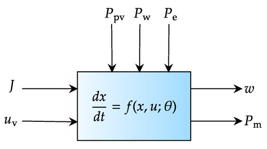
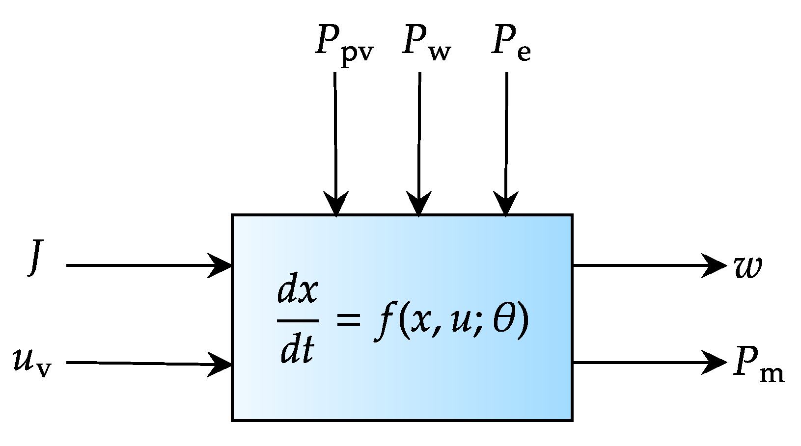
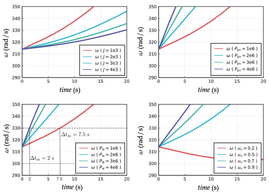
The functional diagram for open-loop simulation is shown in Figure 2. We use open simulation of the model in Equations (4) to (7). We want to see the effect of inertia changes and the injection of solar and wind power into the microgrid. Figure 3 shows deviations in grid frequency due to inertia, solar power, wind power, and hydro power loading conditions, respectively. The figure shows that grid frequency deviations are proportional to the grid inertia and reciprocal to the power injected into the grid.

Figure 2. Functional diagram for model analysis.

Figure 3. Deviations in $\omega$ due to J, $P_{\mathrm{pv}}$, $P_{\mathrm{w}}$ and $u_{\mathrm{v}}$. The deviations in the grid frequency are proportional to the static power injected in the microgrid and the loading of hydro-turbine. $\Delta t_{\mathrm{m}}$ is the maximum allowed discretization time for a controller to maintain the grid frequency.

Figure 3 also shows that for wind power injected into the grid with $P_{\mathrm{w}}=1\mathrm{MW}$, the upper bound for frequency is reached at $t=7.5\mathrm{s}$ and for $P_{\mathrm{w}}=4\mathrm{MW}$ the upper bound is reached at $t=2\mathrm{s}$. The time at which the low or the high bound is reached by the angular frequency is the maximum allowed time for controller $\Delta t_{\mathrm{m}}$ to limit angular velocity within the range $314\pm 5\%\mathrm{rad}/\mathrm{s}$. This provides quantitative information regarding the discretization time used in the control algorithms. For example, for injection of $P_{\mathrm{w}}=4\mathrm{MW}$ into the grid, it would require discretization time of controller, to be less than $2\mathrm{s}$. The rate at which power is injected into the grid is inversely related to the maximum discretization time for the controller.

4.2. Parameter Sensitivity Analysis

Parameter sensitivity analysis can be very useful for seeing variations of the rate of change in states due to the rate of change in parameters over the time-series. From Figure 2, we will consider inputs $P_{\mathrm{pv}}$, $P_{\mathrm{w}}$, $P_{\mathrm{e}}$, $u_{\mathrm{v}}$ with constant values around operating conditions, and parameter J for sensitivity analysis. Hence, inputs $P_{\mathrm{pv}}$, $P_{\mathrm{w}}$, $P_{\mathrm{e}}$, and $u_{\mathrm{v}}$ are also consider as parameters for parameter sensitivity analysis.

The sensitivity ODE for a system with $\frac{dx}{dt}=f\left(x,u;\theta \right)$ is formulated as,

$$\begin{array}{cc}\hfill \frac{d}{dt}\left(\frac{\partial x}{\partial {\theta }_j}\right)& =\left(\frac{\partial f}{\partial x}\right)\left(\frac{\partial x}{\partial {\theta }_j}\right)+\frac{\partial f}{\partial {\theta }_j},\hfill \end{array}$$

and is further simplified with sensitivity ODEs as,

$$\begin{array}{cc}\hfill \frac{d{S}_j}{dt}& =J_{\mathrm{x}}·S_j+F_j,\hfill \end{array}$$

where $J_{\mathrm{x}}$ is the matrix of Jacobians in states, $S_j$ is the sensitivity ODEs of $j^{th}$ parameter and $F_j$ is the parameter derivatives.

We formulate our local sensitivity analysis from parameters $P_{\mathrm{pv}}$, $P_{\mathrm{w}}$, $P_{\mathrm{e}}$, J and $u_{\mathrm{v}}$, and want to see their sensitivities in states $h,{\dot{V}}_{\mathrm{s}},{\dot{V}}_{\mathrm{p}},$ and $\omega$.

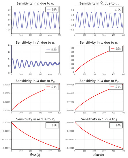
Figure 4 shows sensitivity analysis where the solutions for $S_{\mathrm{j}}$ are plotted over $500$s are plotted over $500\mathrm{s}$. The figure shows $h,{\dot{V}}_{\mathrm{s}}$ and ${\dot{V}}_{\mathrm{p}}$ are less sensitive to $u_{\mathrm{v}}$ as compared to sensitivity in $\omega$, and are periodic overtime with time period $50\mathrm{s}$. The sensitivity in flow rate through the penstock due to turbine valve signal is exponentially decaying towards the solutions indicating regaining of the state’s stability exponentially oscillating over the solutions. The grid frequency $\omega$ is more sensitive to parameter $u_{\mathrm{v}}$.

Figure 4. Local parameter sensitivity analysis.

4.3. Power Injection into the Grid

Real measurements for solar irradiance and wind velocity (The measurement data is for Kjølnes Ring 56, Campus Porsgrunn, University of South-Eastern Norway, 9.6714 longitudes and 59.13814 latitudes.) solar power and wind power, respectively, are taken from www.solarcast.com. The measurement data for consumer load is taken for monthly hourly averaged load for Norway from ENTOS-E. The magnitude of measurement data for electrical demand is modified as per our case study with a microgrid with a power capacity of $6\mathrm{MW}$ keeping the load dynamics preserved in hourly data.

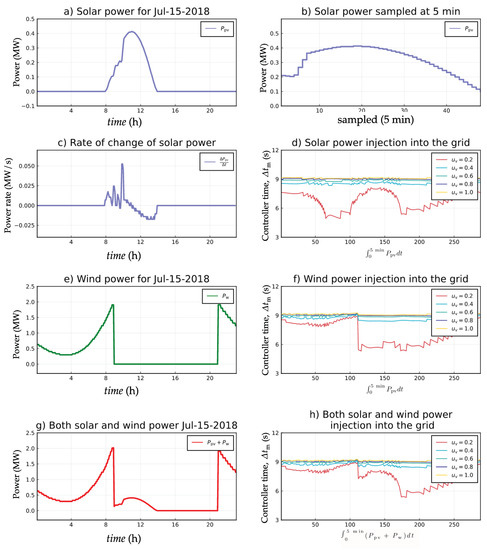
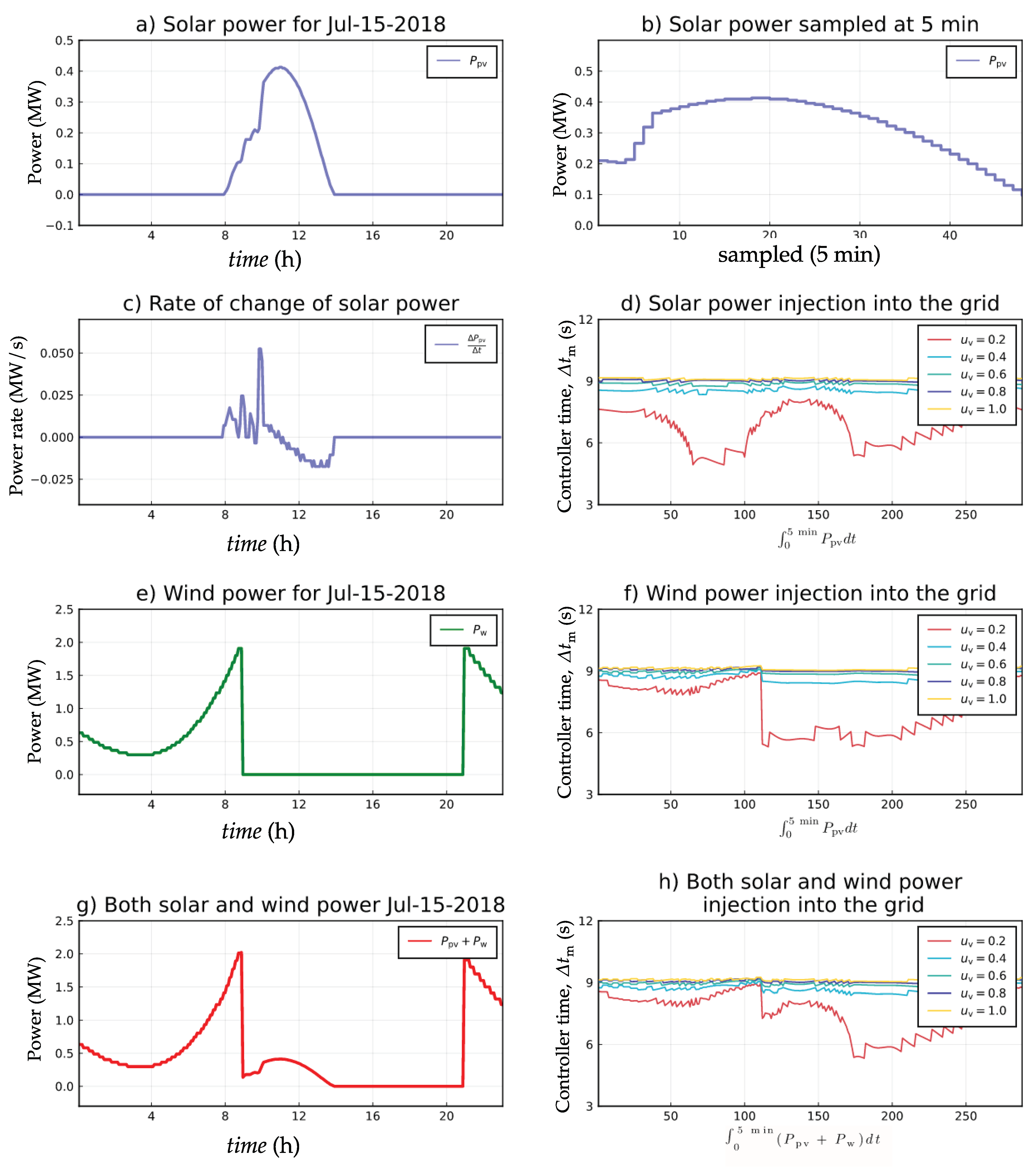
We consider the injection of solar power, wind power, and their combination into the grid. The static wind power comes from grid-based inverters. Figure 5a,e shows solar and wind power, respectively, for a particular day. Similarly, Figure 5b shows solar power sampled at $5\min$ where the value is shown for midday only from 10 a.m. to 2 p.m. A full day consists of 288 data points.

Figure 5. Intermittent power injection into the grid to study limits on $\Delta t_{\mathrm{m}}$.

Our interest is to find the maximum discretization time for controller, $\Delta t_{\mathrm{m}}$, as shown in Figure 3 where grid frequency is satisfied with $\left(300<\omega <330\right)\mathrm{rad}/\mathrm{s}$. $\Delta t_{\mathrm{m}}$ is based on the rate of power injection into the grid and the time at which grid frequency is within the allowed range.

4.3.1. Static Power Injection

Figure 5c shows the rate of change of solar power which is injected into the grid. Figure 5d shows $\Delta t_{\mathrm{m}}$ versus the rate of solar power injection into the grid for different valve positions. In particular, the turbine valve positions during solar power injection do not alter the grid frequency. However, the lower valve positions alter grid frequency and are insignificant in a microgrid with the same scaling of hydro power and solar power plants. The figure shows the discretization time of controllers for higher valve position is around $8\mathrm{s}$ and for lower valve positions is around $5\mathrm{s}$.

Figure 5f shows the discretization time of controllers for different valve positions for a different rate of wind power injection into the grid. We consider wind power sources without inertial impact into the grid. Similarly, Figure 5g shows both solar and wind power injected into the grid, and Figure 5h shows the discretization time of the controllers for different valve positions for a different rate of both solar and wind power injected into the grid.

4.3.2. Inertial Power Injection

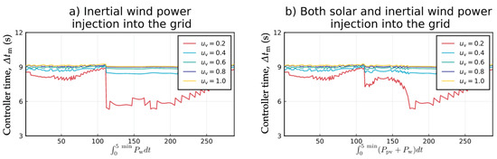
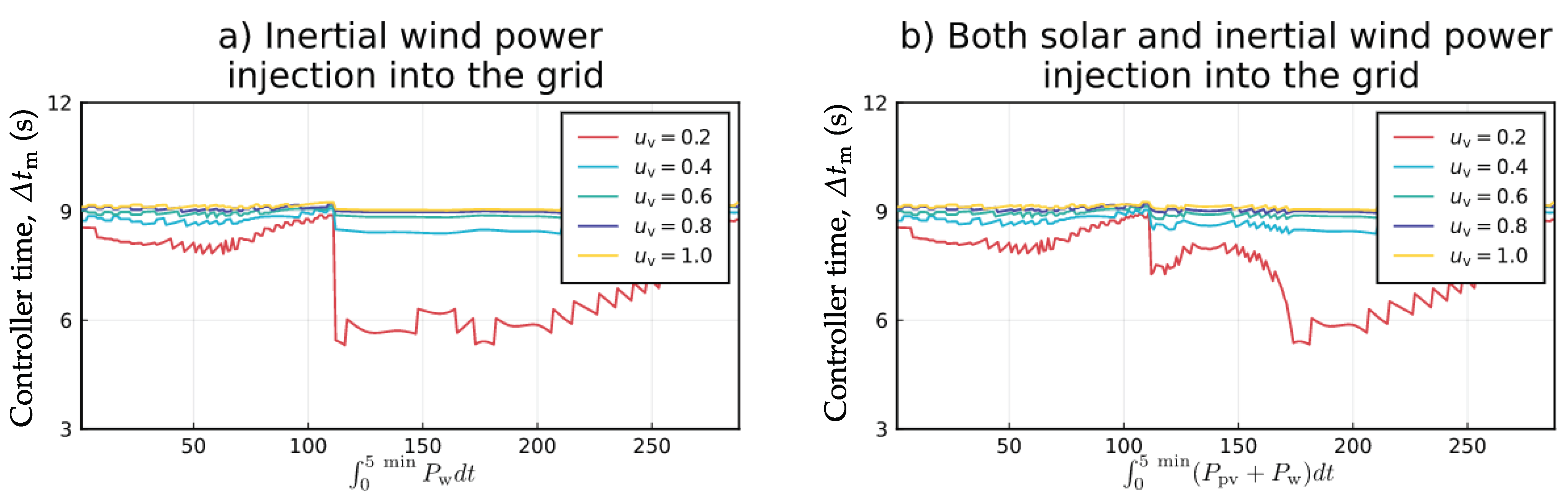
We now consider $J_{\mathrm{w}}$ and $J_{\mathrm{h}}$ as the moment of inertia for wind power plant and hydro power plant, respectively. Figure 6a shows the discretization time of controllers for different valve positions for different rates of both inertial wind power injected into the grid. Figure 6b shows discretization time for both solar and inertial wind power injections into the grid.

Figure 6. Inertial wind power injection into the grid. $\Delta t_{\mathrm{m}}$ is the maximum controller discretization time calculated for power injected at an interval of $5\min$.

Figure 5f,h and Figure 6 shows that inertial power injection into the grid has insignificant effect on $\Delta t_{\mathrm{m}}$.

5. MPC in a Microgrid

A chosen cost function is given as in Equation (10),

$$\begin{array}{ccc}\hfill & \underset{u_k}{\min }\hfill & \hfill J_c=\frac{1}{2}\sum _{k=1}^{N_{\mathrm{p}}}{\left(y_k-r_k\right)}^2+p\Delta u_{k-1}^2\\ \hfill & \mathrm{s}.\mathrm{t}.\hfill \\ \hfill & \hfill & \hfill \frac{dx}{dt}=f\left(x,u,w;\theta \right),\\ \hfill & \hfill & \hfill y=g\left(x,u,v;\theta \right),\\ \hfill & \hfill & \hfill u_{\ell }\le u\le u_{\mathrm{h}},\\ \hfill & \hfill & \hfill \Delta u_{\ell }\le \Delta u\le \Delta u_{\mathrm{h}},\\ \hfill & \hfill & \hfill x_{\ell }\le x\le x_{\mathrm{h}},\end{array}$$

(10)

where subscript ℓ and $\mathrm{h}$ are low and high bounds for inputs, rate of change of inputs, and states. Furthermore, $N_{\mathrm{p}}$ gives the prediction horizon in the optimal control problem (OCP) which is solved for each iteration. p is a scalar weight for tuning the controller. k is the iteration for each sample drawn for solar power, wind power, and consumer load at discretization time of the controller $\Delta t_{\mathrm{c}}$. y is system output/controlled variable, r is reference value, u is control input, $\theta$ is parameter. w and v are process disturbance and measurement noise, respectively.

For our hydropower system connected in microgrid with solar and wind power plant,

$$\begin{array}{cc}\hfill x& =\left(h,{\dot{V}}_{\mathrm{s}},{\dot{V}}_{\mathrm{p}},\omega \right)\hfill \\ \hfill y& =P_{\mathrm{e}}\hfill \\ \hfill u& =u_{\mathrm{v}}\hfill \\ \hfill r& =P_{\ell }.\hfill \end{array}$$

5.1. Deterministic MPC

5.1.1. Without Process Disturbance and Measurement Noise

For prediction analysis, first, we consider both the model and the plant with the same mathematical equations and without the inclusion of process disturbance and measurement noise. Table 2 shows parameters and initial conditions for an MPC controller with UKF as an estimator. The controller discretization time $\Delta t_{\mathrm{c}}$ is chosen based on parameter sensitivity analysis and rate of power injection into the grid satisfying grid frequency for $\left(314\pm 5\%\right)\mathrm{rad}/\mathrm{s}$. For a controller maintaining grid frequency within the limits holds true for $\Delta t_{\mathrm{c}}\le \Delta t_{\mathrm{m}}$.

Table 2. Controller specifications.

Parameters and Initial Conditions	Symbols	Values
Prediction horizon	$N_{\mathrm{p}}$	5
Normalized tuning parameter for input	p	$0.1$
Controller discretization time	$\Delta t_{\mathrm{c}}$	$10\mathrm{s}$
Initial conditions for states	$h\left(0\right),{\dot{V}}_{\mathrm{s}}\left(0\right)$$,{\dot{V}}_{\mathrm{p}}\left(0\right),\omega \left(0\right)$	$20\mathrm{m},2{\mathrm{m}}^3/\mathrm{s},4{\mathrm{m}}^3/\mathrm{s},314\mathrm{rad}/\mathrm{s}$
Bounds for water mass oscillations inside surge tank	$h_{\ell }\le h\le h_{\mathrm{h}}$	$0<h\le 40\mathrm{m}$
Bounds for flow rate through surge tank	${\dot{V}}_{\mathrm{s},\ell }\le {\dot{V}}_{\mathrm{s}}\le {\dot{V}}_{\mathrm{s},\mathrm{h}}$	$-4{\mathrm{m}}^3/\mathrm{s}<h\le 4{\mathrm{m}}^3/\mathrm{s}$
Bounds for discharge through penstock	${\dot{V}}_{\mathrm{p},\ell }\le h\le {\dot{V}}_{\mathrm{p}}\le {\dot{V}}_{\mathrm{p},\mathrm{h}}$	$0<h\le 4{\mathrm{m}}^3/\mathrm{s}$
Bounds for grid frequency	${\omega }_{\ell }\le \omega \le {\omega }_{\mathrm{h}}$	$300\mathrm{rad}/\mathrm{s}<\omega \le 330\mathrm{rad}/\mathrm{s}$
Bound for valve signal	$u_{\mathrm{v},\ell }<u_{\mathrm{v}}\le u_{\mathrm{v},\mathrm{h}}$	$0<u_{\mathrm{v}}\le 1$
Rate of change of valve signal	${\dot{u}}_{\mathrm{v},\ell }\le \Delta {\dot{u}}_{\mathrm{v}}\le {\dot{u}}_{\mathrm{v},\mathrm{h}}$	$-0.8{\mathrm{s}}^{-1}<{\dot{u}}_{\mathrm{v}}\le 0.8{\mathrm{s}}^{-1}$
Process distrubances with mean $\overline{w}$ and co-variance W	$w\sim \mathcal{N}\left(\overline{w},W\right)$	$\overline{w}=0$ and $W=\mathrm{diag}\left(0.01,0.04,0.04,0.01\right)$
Measurement noises with mean $\overline{v}$ and co-variance V	$v\sim \mathcal{N}\left(\overline{v},V\right)$	$\overline{v}=0$ and $V=\mathrm{diag}\left(0.1\right)$
States co-variance for UKF	X	$X=100·W$

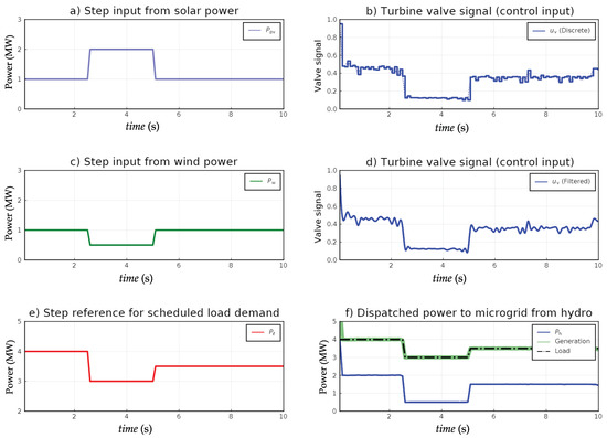
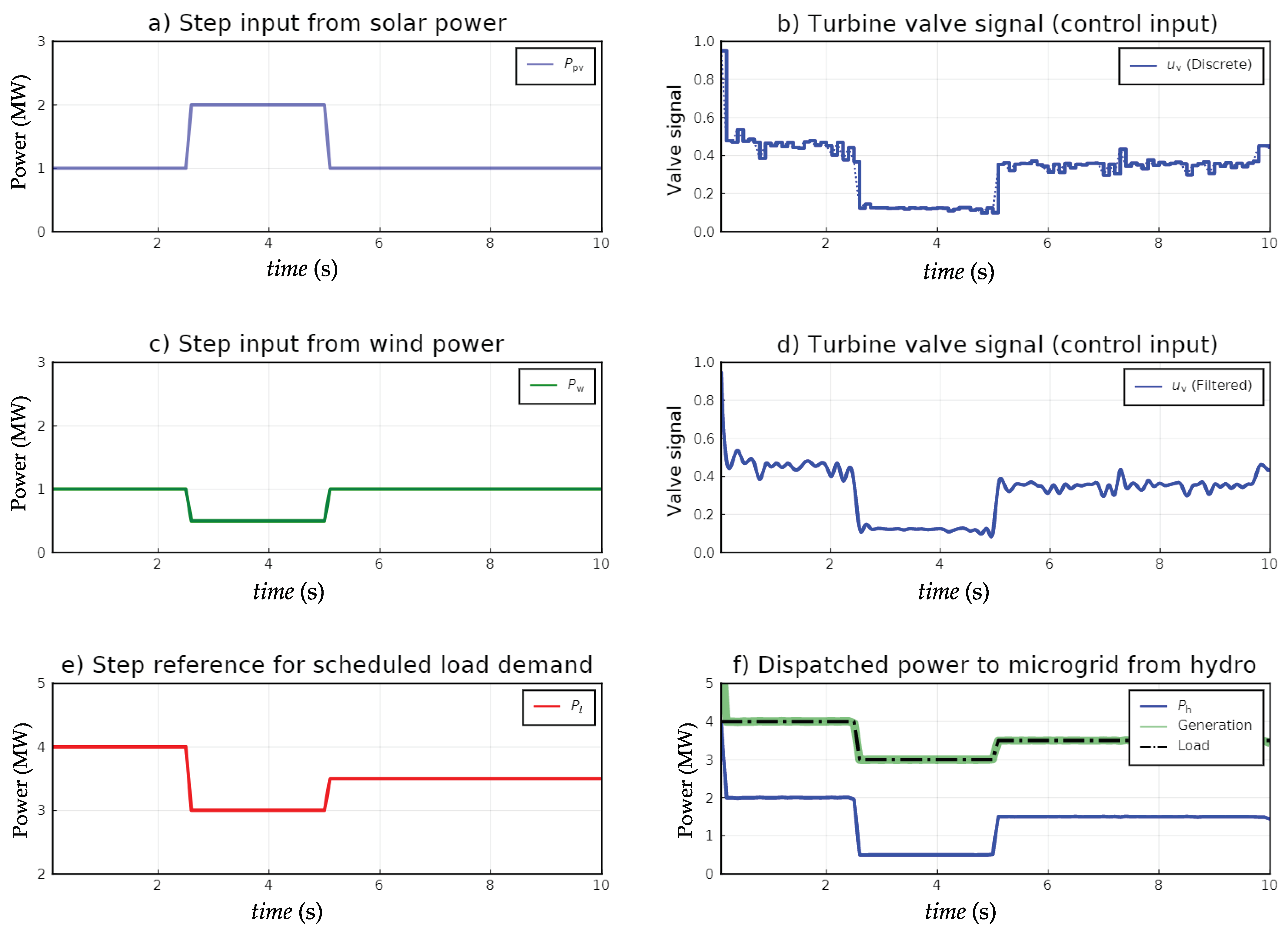
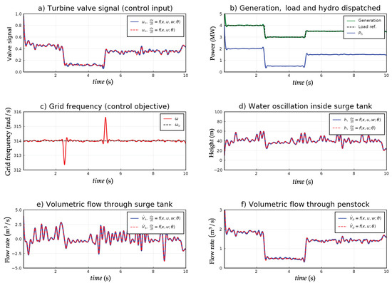
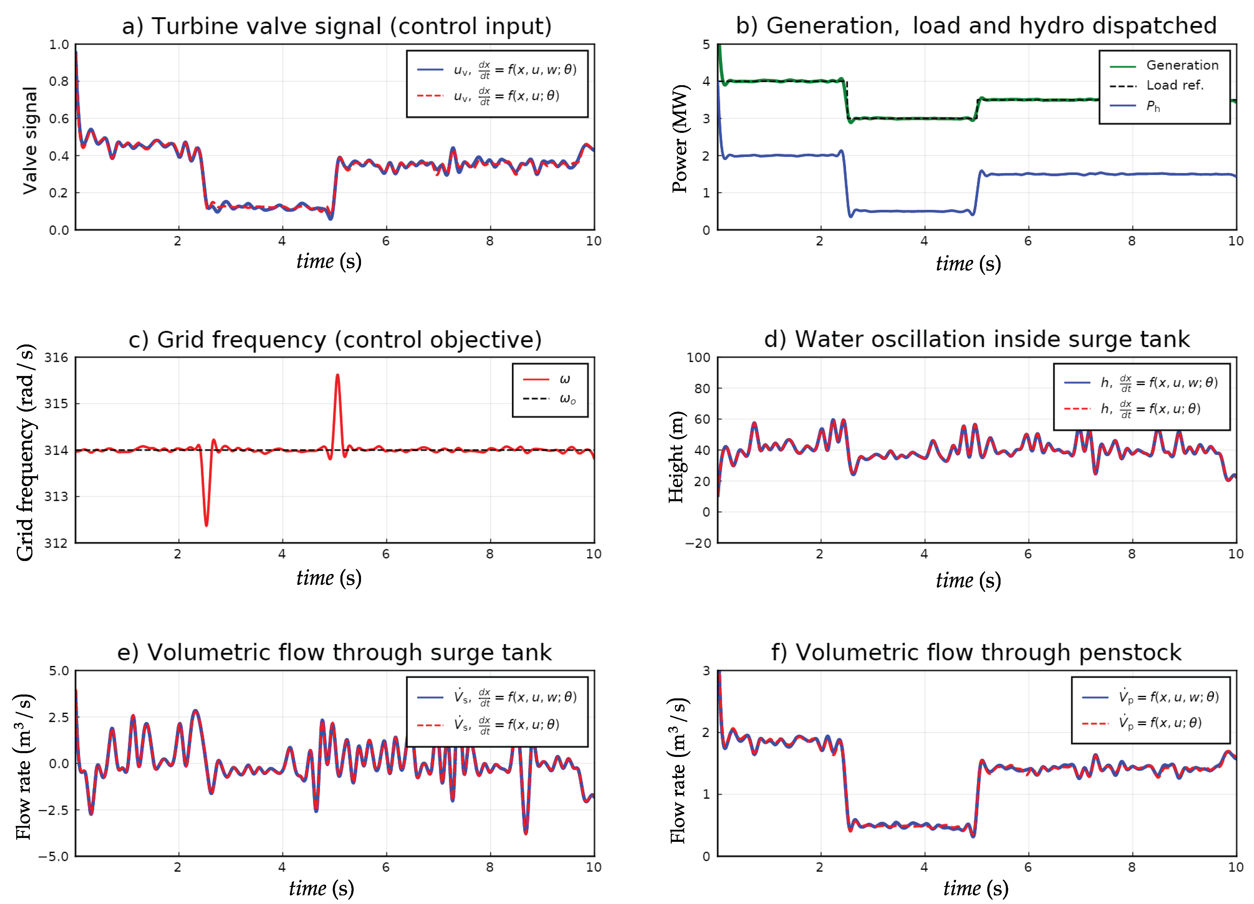
Figure 7 shows step generation input from solar power, wind power, schedule load setpoints, controlled input, and states.

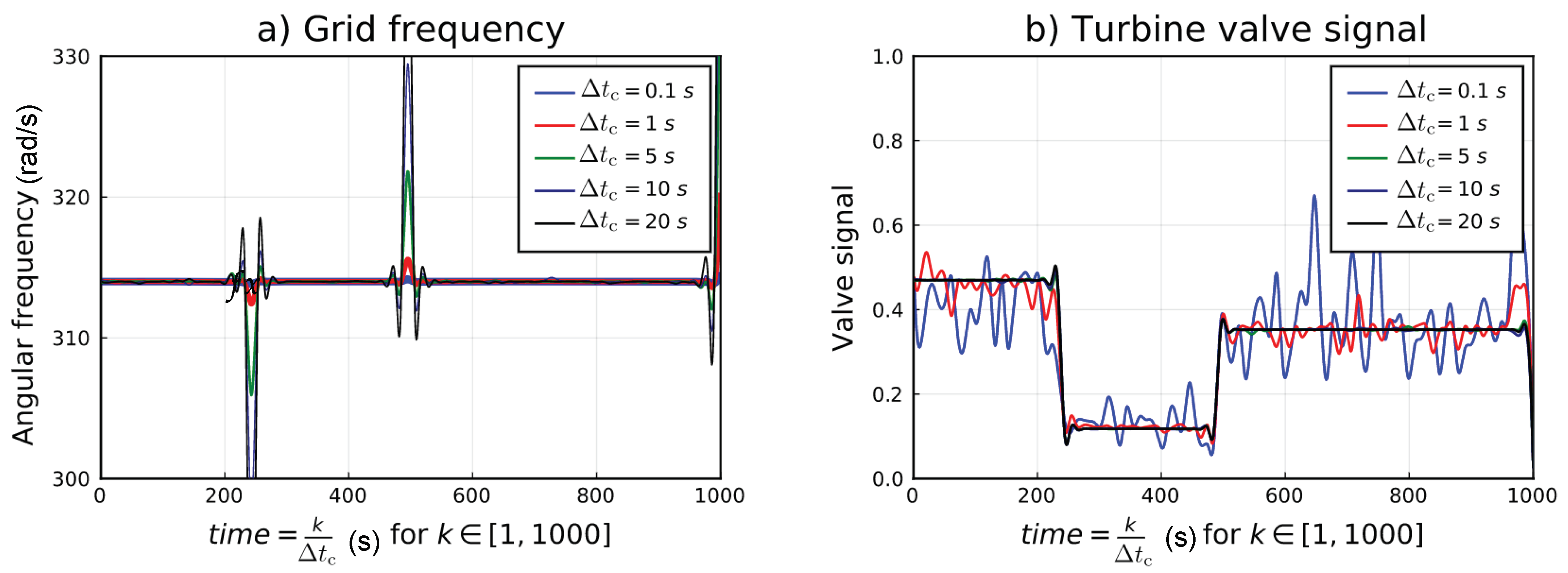
Figure 7. Setpoint tracking of scheduled load using step input from solar and wind power. Both the plant and model are represented by mathematical equations. The control input $u_{\mathrm{v}}$ from the OCP is generated for grid frequency to be exactly at $314\mathrm{rad}/\mathrm{s}$ for $\Delta t_{\mathrm{c}}=0.1\mathrm{s}$. However, the actual plant is now out of control for the next $0.1\mathrm{s}$ at which period grid frequency fluctuates. Figure 7 shows the instantaneous (interpolated) dynamics of turbine valve signal which maintain frequency within the required limit as shown in Figure 8a with the blue color.

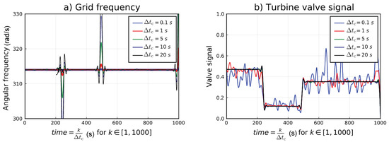
Figure 7b shows grid frequency for different $\Delta t_{\mathrm{c}}$. As the discretization time for MPC increased grid frequency fluctuates out of the range. For a typical value of $\Delta t_{\mathrm{c}}=20\mathrm{s}$, the grid frequency is not maintained within the range. The controller performs better when $\Delta t_{\mathrm{c}}=0.1\mathrm{s}$. Similarly, Figure 7c shows the valve signal of the turbine for different discretization time. Thus, a very low value of $\Delta t_{\mathrm{c}}$ would require the turbine’s valve with a fast response time.

5.1.2. With Process Disturbance and Measurement Noise

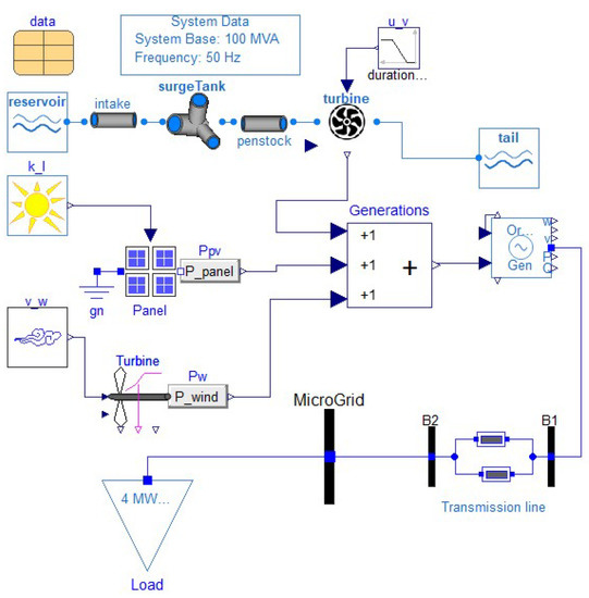
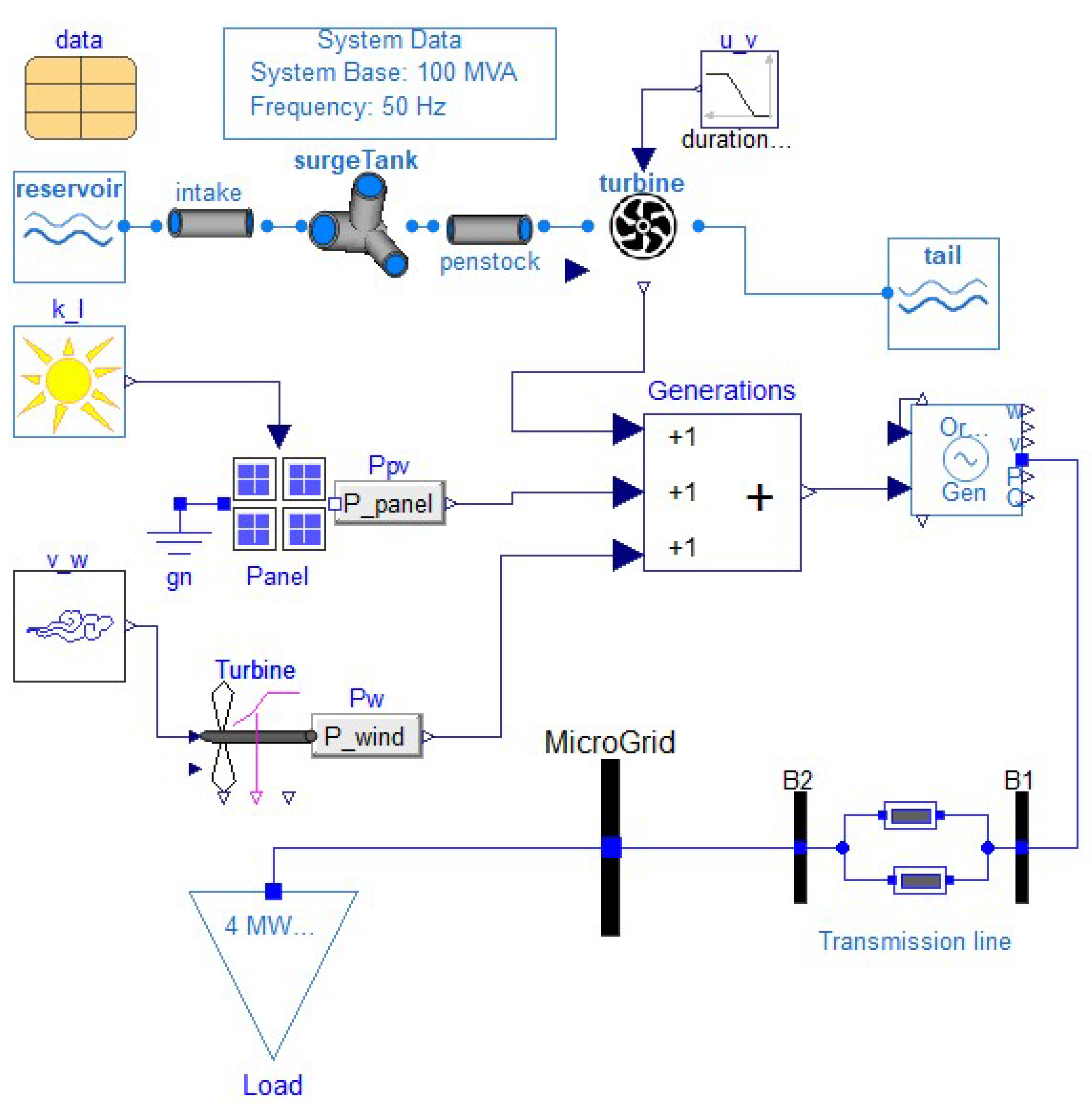
We now consider white noise added to the process and measurement equations. For emulation of the real plant, we consider a model developed in OpenModelica [16] using Modelica [17] libraries. The Modelica language is chosen based on the current state-of-the-art for simulation of multiphysical systems. The choice of language is based on an open-source platform, equation-based modeling possibilities, extensive contributors in the development of the language and its libraries, ease-of-use, interfaces to high-level languages such as Julia and Python [18]. We are using Modelica libraries—OpenHPL [19] for modeling hydro power and pump operations, OpenIPSL [20] for electrical generation, transmission, and distribution, PhotoVoltaics [21] for solar power plants, and WindPowerPlants [22] for wind power plants. In the Modelica language, models can be developed using Differential Algebraic Equations (DAEs) which are solved with high order, efficient solvers. Because of the DAEs representation, the solutions of the algebraic variables are readily accessible. The simulated output is considered to be the real plant measurements by adding white noise as measurement noise. For state estimation and updating states for the control horizon, we use the model developed in OpenModelica as shown in Figure 9.

Figure 9. Simulation model developed in OpenModelica using Modelica libraries, OpenHPL, OpenIPSL, PhotoVoltaics, and WindPowerPlants.

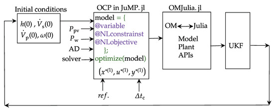
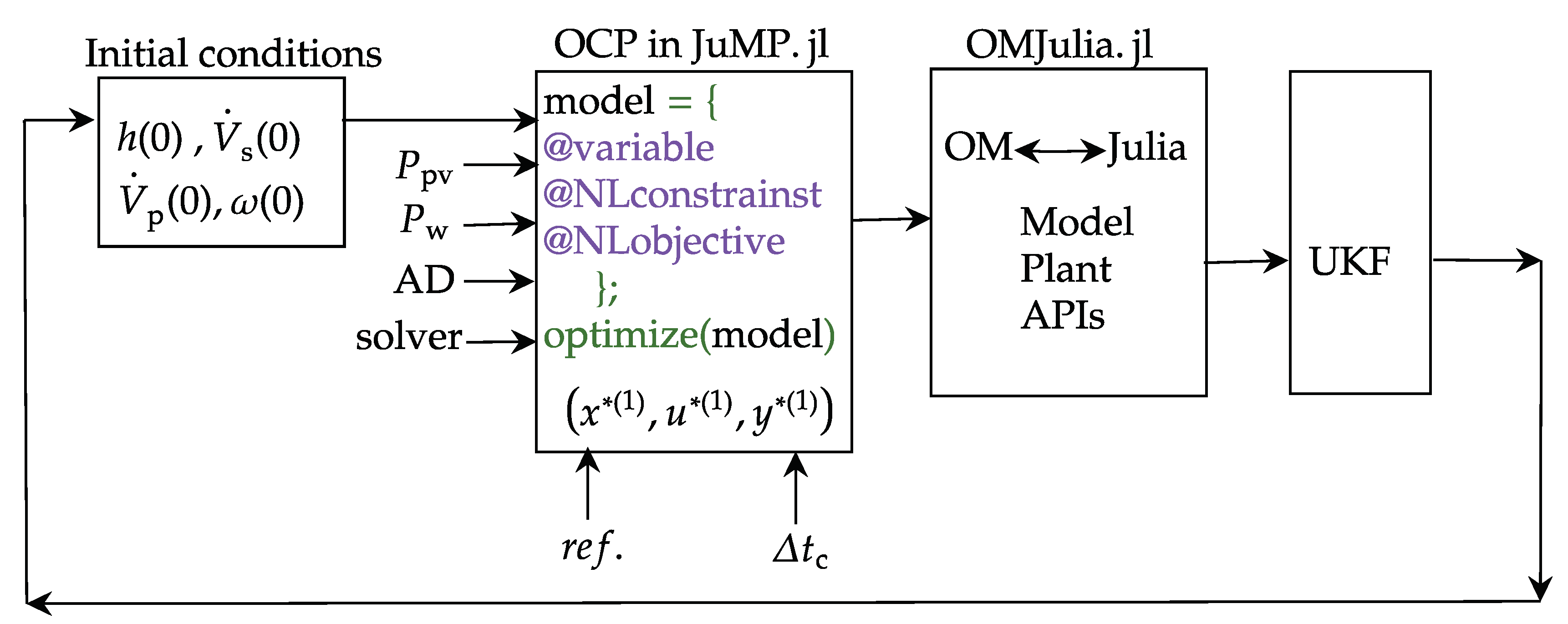
The internal structure of OCP is formulated in the Julia language [23] using JuMP.jl, a Julia package for modeling optimization problem [24], as shown in Figure 10. JuMP provides an easy way of describing optimization problems containing linear and non-linear constraints. JuMP also supports automatic differentiation (AD) using package ForwardDiff.jl [25] which is a most useful property rarely supported by other modeling languages. Several open-source solvers are available for solving models described in JuMP. Our choice of JuMP solver is Ipopt.We have used models developed in Modelica for both model and plant. OMJulia [26] is an OpenModelica-Julia interface providing application programming interfaces (APIs) for advance model analysis in Julia. The difference in measurements from plant and simulated outputs from the model is fed into UKF to estimate the next states and outputs for OCP.

Figure 10. Internal structure of optimal control problem (OCP) formulated in JuMP.jl. $\left(x^{\ast \left(1\right)},u^{\ast \left(1\right)},y^{\ast \left(1\right)}\right)$ represents first optimal values of states, inputs and outputs.

Table 3 describes model use for real plant and mathematical model for solving control optimization.

Table 3. Models used for real plant and control.

Real Plant	Control Model
1. Developed in Modelica $$\frac{dx}{dt}=f\left(x,z,u;\theta \right)$$ $$0=g\left(x,z,u,w;\theta \right)$$ $$y=h\left(x,z,u,v;\theta \right),$$ where differential variables, algebraic variables, inputs, white noise, parameters and outputs, respectively. The model consists of DAEs.	1. Developed in Julia $$\frac{dx}{dt}=f\left(x,u,w;\theta \right)$$ $$y=h\left(x,u,v;\theta \right),$$ where x is a state obtained by reducing conservation equations using algebraic variables. The model consists of ODEs.
2. Use for emulating measurements, states estimation and updating states.	2. Use for formulating model constraints for cost function used in MPC
3. Modelica libraries: OpenHPL, OpenIPSL, Photovoltaics and WindPowerConversionSystems for modeling hydro powers, electrical systems, solar and wind power plants, respectively.	3. Only hydro power and aggregate model is considered
4. Higher order model with automatic discretization for solving model equations.	4. Euler discretization

Figure 11 shows control input and output when process disturbance and measurement noise are included. The scheduled load is considered to be measurement output used for estimation of states $h,{\dot{V}}_{\mathrm{s}},{\dot{V}}_{\mathrm{p}}\mathrm{and}\omega$ using UKF. The effect in the control inputs and outputs are almost the same in the case of models with and without process disturbances and measurement noises.

Figure 11. Setpoint tracking of scheduled load with process disturbance and measurement noise, and step change in solar and wind power.

Furthermore, we will consider the model without process disturbance and control noise for further analysis throughout the paper. Similarly, we assume $\Delta t_{\mathrm{c}}=1\mathrm{s}.$

5.1.3. With Real Measurements

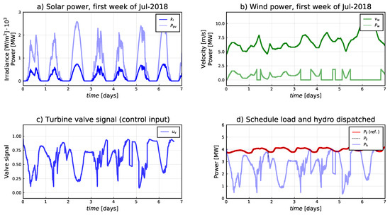
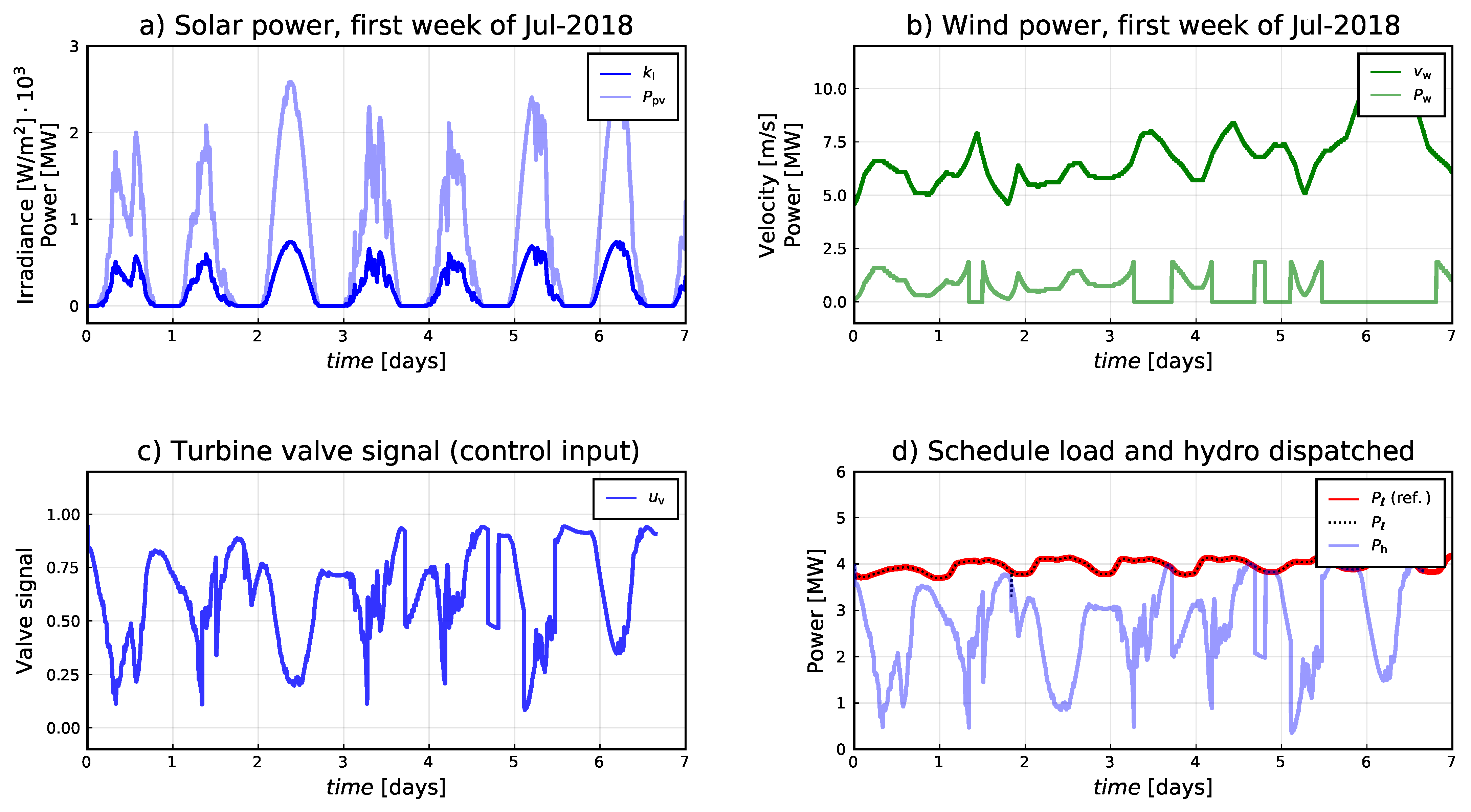
Figure 12a,b shows solar irradiance and wind velocity with their respective power productions. When the wind velocity $v_{\mathrm{w}}>7\mathrm{m}/\mathrm{s}$, wind turbines are shut down and power production from wind is zero. Similarly, Figure 12c shows the control inputs for setpoint tracking of the scheduled load as shown in Figure 12d. The dispatched hydro power for balancing load and generation is shown in Figure 12d.

Figure 12. Setpoint tracking of scheduled load using real measurements for solar power, wind power, and consumer load.

5.1.4. Pump-Turbine Operations

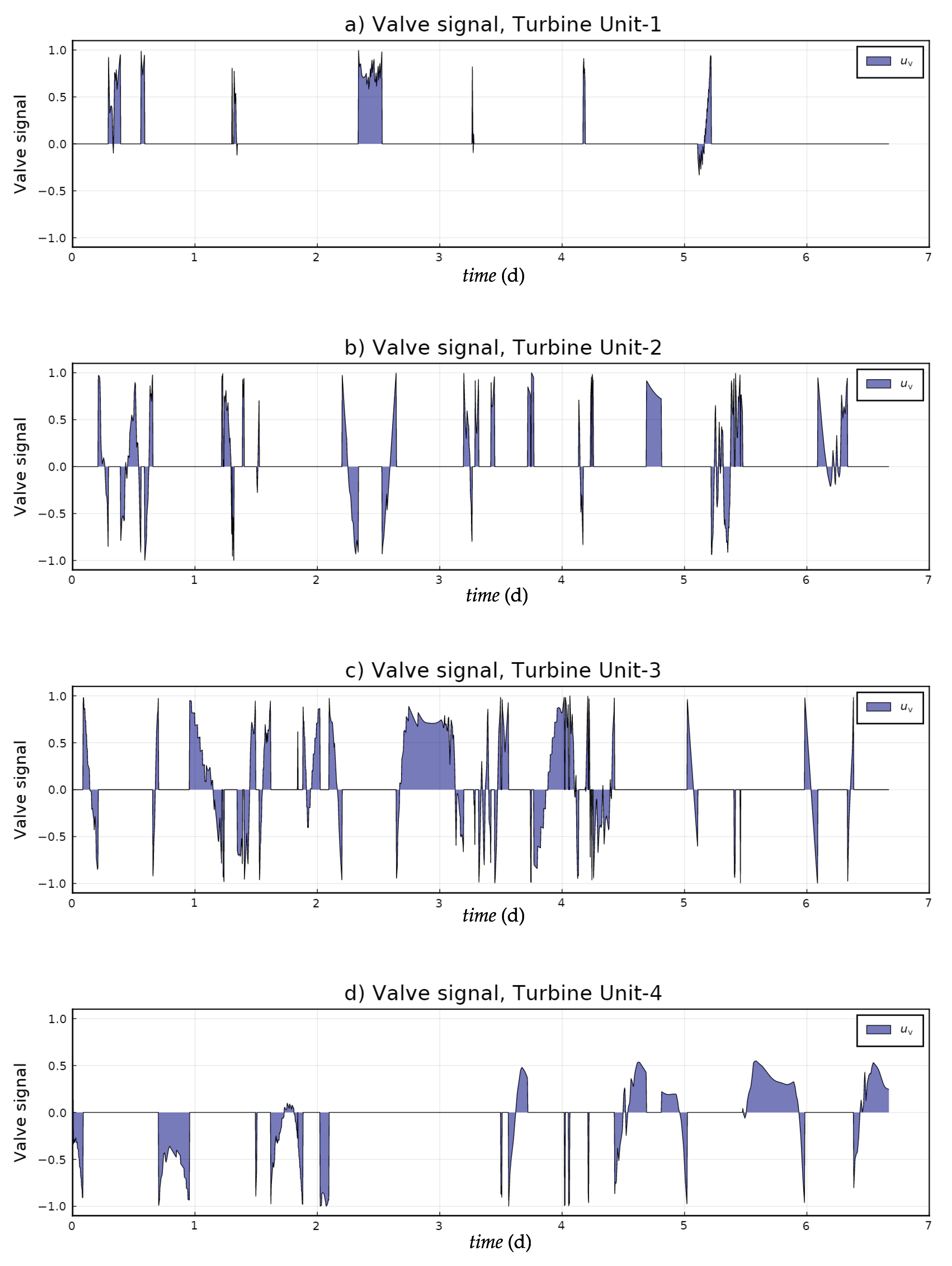
The motoring and generating operation of the 4-units of the hydro-turbine is shown in Figure 13. We consider pumping and turbine as mirror dynamics for pump-storage hydropower.

Figure 13. Pump-turbine operations of hydro power. $u_{\mathrm{v}}\in \left(0,1\right)$ for each of the pump-turbines. Unit 1 gets first priority to run either in generating or motoring mode. If unit 1 operates in generating mode near full load, then after it reaches full load unit 2 starts to operate and balance the generation and load. And so on. The same applies to motoring mode.

5.2. Stochastic Analysis

Section 5.1 explored deterministic MPC. In practice, solar power, wind power, and consumer load are stochastic. Thus, we want to study how deterministic MPC handles stochastic inputs from solar power, wind power, and consumer load. For future prediction, stochastic behavior can be studied using different random scenarios. These scenarios are based on the future prediction of solar power, wind power, and scheduled load, using the state-space model and/or confined Weibull and normal distributions.

5.2.1. State-Space Model

A basic structure of state-space model for stochastic processes is represented by three components, trend $\mu$, slope $\nu$, and seasonality $\gamma$ as,

$$\begin{array}{cc}\hfill y_{\mathrm{t}}& ={\mu }_{\mathrm{t}}+{\gamma }_{\mathrm{t}}+{\epsilon }_{\mathrm{t}}\hfill \end{array}$$

(11)

$$\begin{array}{cc}\hfill {\mu }_{\mathrm{t}+1}& ={\mu }_{\mathrm{t}}+{\nu }_{\mathrm{t}}+{\xi }_{\mathrm{t}}\hfill \end{array}$$

(12)

$$\begin{array}{cc}\hfill {\nu }_{\mathrm{t}+1}& ={\nu }_{\mathrm{t}}+{\zeta }_{\mathrm{t}}\hfill \end{array}$$

(13)

$$\begin{array}{cc}\hfill {\gamma }_{\mathrm{t}+1}& =\sum _{j=1}^{s-1}{\gamma }_{\mathrm{t}+1-j}+{\omega }_{\mathrm{t}},\hfill \end{array}$$

(14)

where ${\epsilon }_{\mathrm{t}}\sim N\left(0,{\sigma }_{\epsilon }^2\right)$, ${\xi }_{\mathrm{t}}\sim N\left(0,{\sigma }_{\xi }^2\right)$, ${\zeta }_{\mathrm{t}}\sim N\left(0,{\sigma }_{\zeta }^2\right)$, and ${\omega }_{\mathrm{t}}\sim N\left(0,{\sigma }_{\omega }^2\right)$. s is the seasonality period. For $s=2$ we can represent Equations (11)–(14) by a state-space model as,

$$\begin{array}{cc}\hfill y_{\mathrm{t}}& =\left[\begin{array}{ccc}1& 0& 1\end{array}\right]{\alpha }_{\mathrm{t}}+{\epsilon }_{\mathrm{t}},{\epsilon }_{\mathrm{t}}\sim N\left(0,{\sigma }_{\epsilon }^2\right)\hfill \end{array}$$

(15)

$$\begin{array}{cc}\hfill {\alpha }_{\mathrm{t}+1}& =\left[\begin{array}{ccc}1& 1& 0\\ 0& 1& 0\\ 0& 0& 1\end{array}\right]{\alpha }_{\mathrm{t}}+\left[\begin{array}{ccc}1& 1& 0\\ 0& 1& 0\\ 0& 0& 1\end{array}\right]{\eta }_{\mathrm{t}},{\eta }_{\mathrm{t}}\sim N\left(\left[\begin{array}{c}0\\ 0\\ 0\end{array}\right],\left[\begin{array}{ccc}{\sigma }_{\xi }^2& 0& 0\\ 0& {\sigma }_{\zeta }^2& 0\\ 0& 0& {\sigma }_{\omega }^2\end{array}\right]\right),\hfill \end{array}$$

(16)

where y is the measurement output modeled with white noise characterized by variance ${\sigma }_{\epsilon }^2$. Here, $\alpha =\left(\mu ,v,\gamma \right)$ is the state vector, and $\eta =\left(\xi ,\zeta ,\omega \right)$ is the disturbance vector. The respective variances for disturbances are ${\sigma }_{\xi }^2,{\sigma }_{\zeta }^2$ and ${\sigma }_{\omega }^2.$ Based on the seasonality factor s, the state-space matrices change sizes. Equations (15) and (16) are used for future prediction and scenarios generation.

We are using StateSpaceModels.jl [27] for stochastic prediction and scenarios generation.

5.2.2. Weibull and Normal Distribution

A parameterized Weibull distribution function is represented by Equation (17).

$$f\left(x\right)=\left\{\begin{array}{cc}\frac{k}{\lambda }{\left(\frac{x}{\lambda }\right)}^{k-1}{e}^{-{\left(\frac{x}{\lambda }\right)}^k}\hfill & x\ge 0\hfill \\ 0\hfill & x<0\hfill \end{array}\right.,$$

(17)

where $k\in \left(0,+\infty \right)$ and $\lambda \in \left(0,+\infty \right)$ are denoted as shape and scale parameters, respectively. Similarly, $x\in \left[0,+\infty \right)$ is the positive infinite space. However, we want to predict the solar irradiance for a day. Thus, an infinite space is converted into $24\mathrm{h}$ confined space. This can be done with the help of space-relaxation parameters as $x\in \left(\alpha ,\beta \right]$ where $\beta >\alpha$ and $\alpha ,\beta \in \left[0,+\infty \right)$.

Similarly, a parameterized Normal distribution function is represented by Equation (18),

$$f\left(x\right)=\frac{1}{\sigma \sqrt{2\pi }}{e}^{-\frac{1}{2}{\left(\frac{x-\mu }{\sigma }\right)}^2},$$

(18)

where $\mu$ and $\sigma$ are mean and standard deviation and $\mu ,x\in \mathbb{R}$ and ${\sigma }^2>0$. The infinite real space is converted to a confined space $x\in \left[\alpha ,\beta \right]$ where $\beta >\alpha$ and $\alpha ,\beta \in \left(-\infty ,+\infty \right)$ where normal distribution can be used for predicting solar irradiance for a complete day of $24\mathrm{h}.$

5.2.3. Relaxation Parameters $\alpha ,\beta$

The relaxation parameters can be found using the least square errors approximation between measurements and calculations from analytical distribution function in a confined space of $x\in \left[\alpha ,\beta \right]$ converted into a space of $24\mathrm{h}.$

If $k_{\mathrm{I}}$ is the solar irradiance and t is a confined time of a day in a year $t\in \left(0,24\right]$ then expressions for solar irradiance using the Weibull distribution is given as,

$$k_{\mathrm{I}}=\frac{k}{\lambda }{\left(\frac{\beta t}{24\lambda }\right)}^{k-1}{e}^{-{\left(\frac{\beta t}{24\lambda }\right)}^k},$$

and for the normal distribution is given as,

$$k_{\mathrm{I}}=\frac{1}{\sigma \sqrt{2\pi }}{e}^{-\frac{1}{2}{\left(\frac{\frac{\beta t}{24}-\mu }{\sigma }\right)}^2}.$$

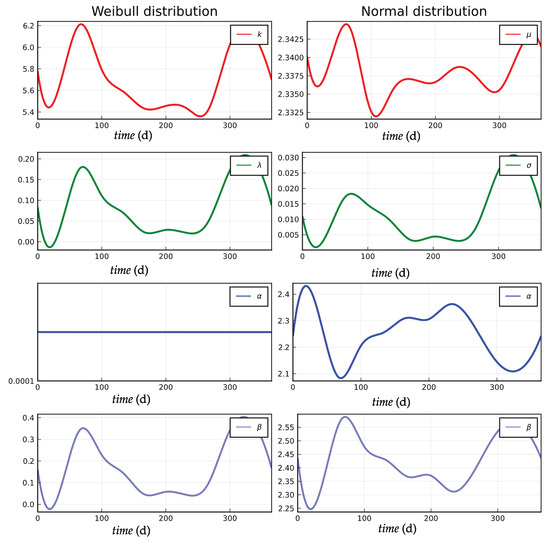
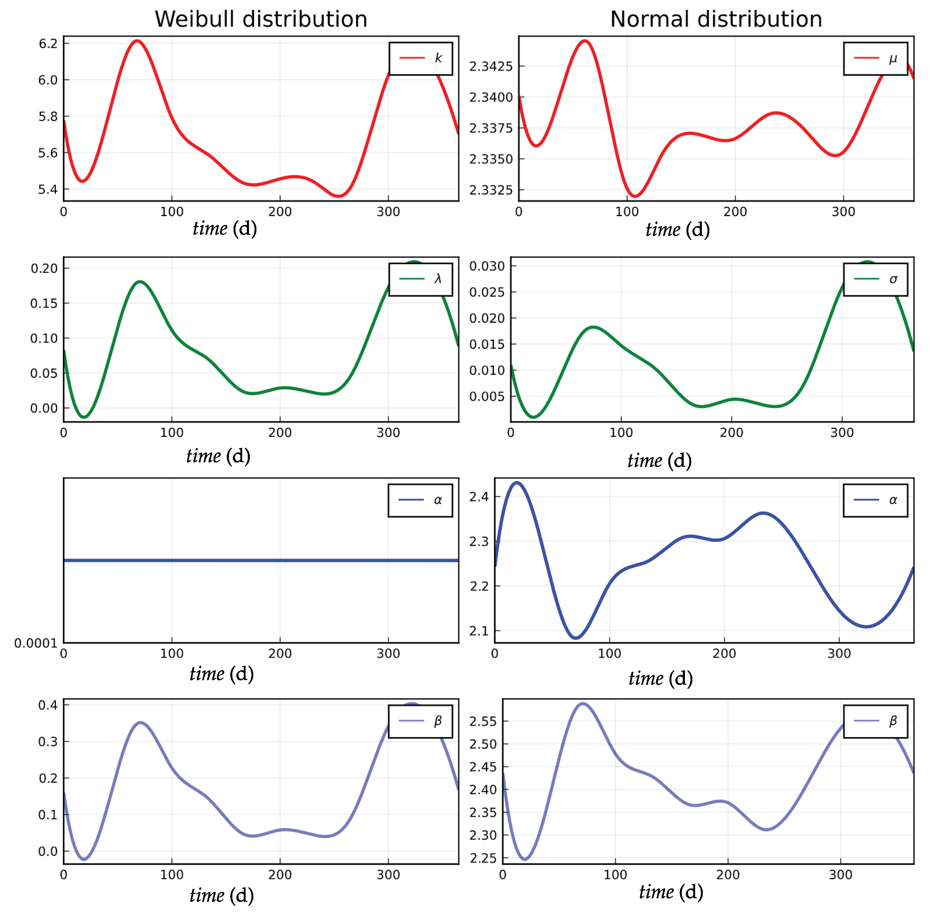
The yearly parameter space for predicting solar irradiance for a particular day using both the Weibull and the normal distribution are given in Figure 14.

Figure 14. Yearly parameters spaces for confined Weibull and normal distributions.

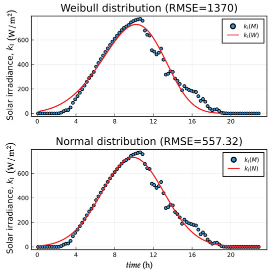
Figure 15 shows irradiance measured on 1 July 2018 fitted to the Weibull and the normal distributions.

Figure 15. Solar irradiance prediction using Weibull and normal distributions for July-01-2018. Root mean square errors (RMSE) shows that the normal distribution is better than Weibull distribution. For the Weibull distribution, $\left(k,\lambda ,\alpha ,\beta \right)=\left(5.25,2.7\times {10}^{-3},8.7\times {10}^{-4},4.7\times {10}^{-3}\right)$, and for the normal distribution $\left(\mu ,\sigma ,\alpha ,\beta \right)=\left(1.9\times {10}^{-4},5.4\times {10}^{-4},1.8\times {10}^{-3},-2\times {10}^{-3}\right)$.

A similar strategic approach can be applied for the prediction of schedule load for a particular day. A yearly parameter space can be generated for schedule load using past data.

However, the concept of using Weibull and normal distribution for the prediction of wind velocity for a particular day is out of the scope of this paper.

5.3. Effect of Shadows

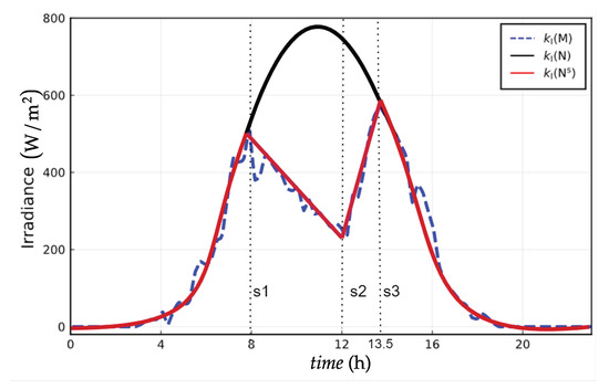
Figure 15 shows irradiance for a day with a clear sky. The effect of shadow cannot be modeled using Weibull and normal distribution. A more rigorous prediction algorithm can be developed to study the effect of shadowing throughout the day.

Figure 16 shows solar irradiance on 2 July 2018. The solar irradiance for the day consists of two shadow events, $s1-s2$ and $s2-s3$. For event $s1-s2$, $s1$ is starting time and $s2$ is the ending time. The starting and the ending time of the shadow event should be known prior to any particular day. In practice, an estimation engineer should predict $s1$ and $s2$ based on the cloud information on that particular day a few hours before the shadow event takes place. More importantly, for better prediction, the estimation engineer should update local information about the clouds.

Figure 16. Solar irradiance fitted to normal distribution. Two shadow events (clouds) are considered between $s1$ and $s2$, and $s2$ and $s3$. $k_{\mathrm{I}}\left(M\right)$ is the measured irradiance, $k_{\mathrm{I}}\left(N\right)$ is the irradiance fitted with normal distribution, and $k_{\mathrm{I}}\left(N^{\mathrm{s}}\right)$ is the irradiance with considering two shadow events.

For a total time of $24\mathrm{h}$ in a day, solar irradiance for initial $8\mathrm{h}$ and from time $s3$ to $23\mathrm{h}$ can be fitted with Weibull or normal distribution choosing parameters from Figure 14 for 2 July 2018; this prediction is the solar irradiance on a clear sky for that particular day. From time $s1=8\mathrm{h}$ to $s2=12\mathrm{h}$ and from time $s2=12\mathrm{h}$ to $s3=13.5\mathrm{h}$, the solar irradiance is fitted with a straight line. The prediction can be updated with higher order polynomials with the updated information by the estimation engineer.

5.4. Generating Future Scenarios

For the stochastic analysis, we generate scenarios using Monte Carlo methods and $95\%$ confidence intervals. Scenarios are generated for a day head prediction from the state-space model or Weibull distribution using past measurement data.

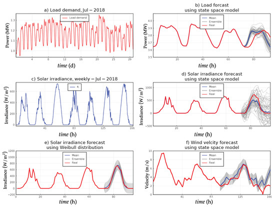
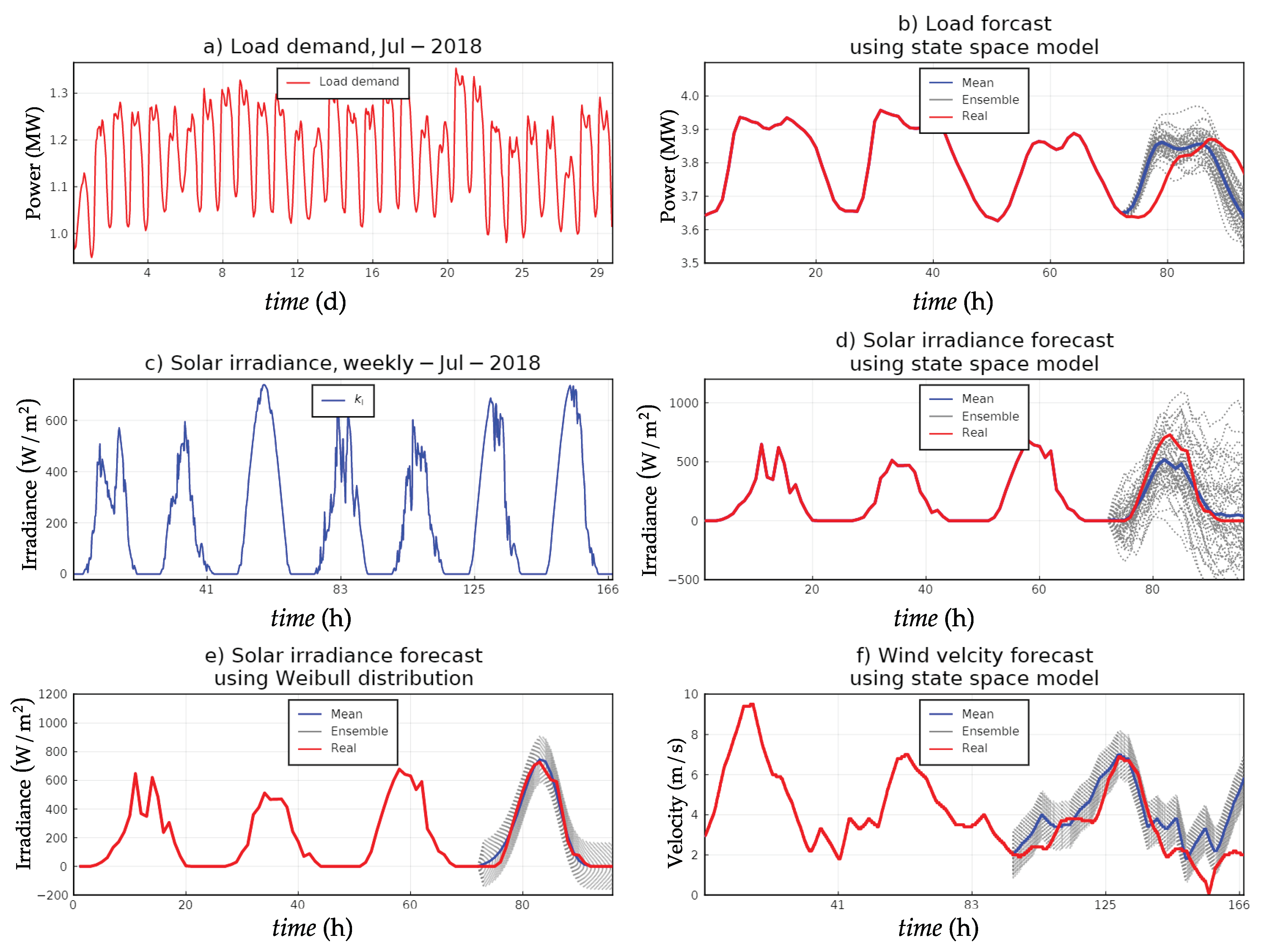
Figure 17a shows a monthly load demand. The load demands on the weekdays are higher as compared to the weekend. Figure 17b shows forecasted load for a day ahead using past weekly data using the state-space model. 50 scenarios are generated using Monte Carlo simulation. Similarly, Figure 17d shows solar irradiance forecast using state-space model and the scenarios are generated based on Monte Carlo simulation. Figure 17e,f show scenarios generations using 95% confidence interval for solar irradiance and wind velocity.

Figure 17. Forecasts for consumer load, solar irradiance, and wind velocity.

Stochastic Analysis of Deterministic MPC

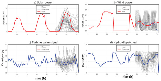
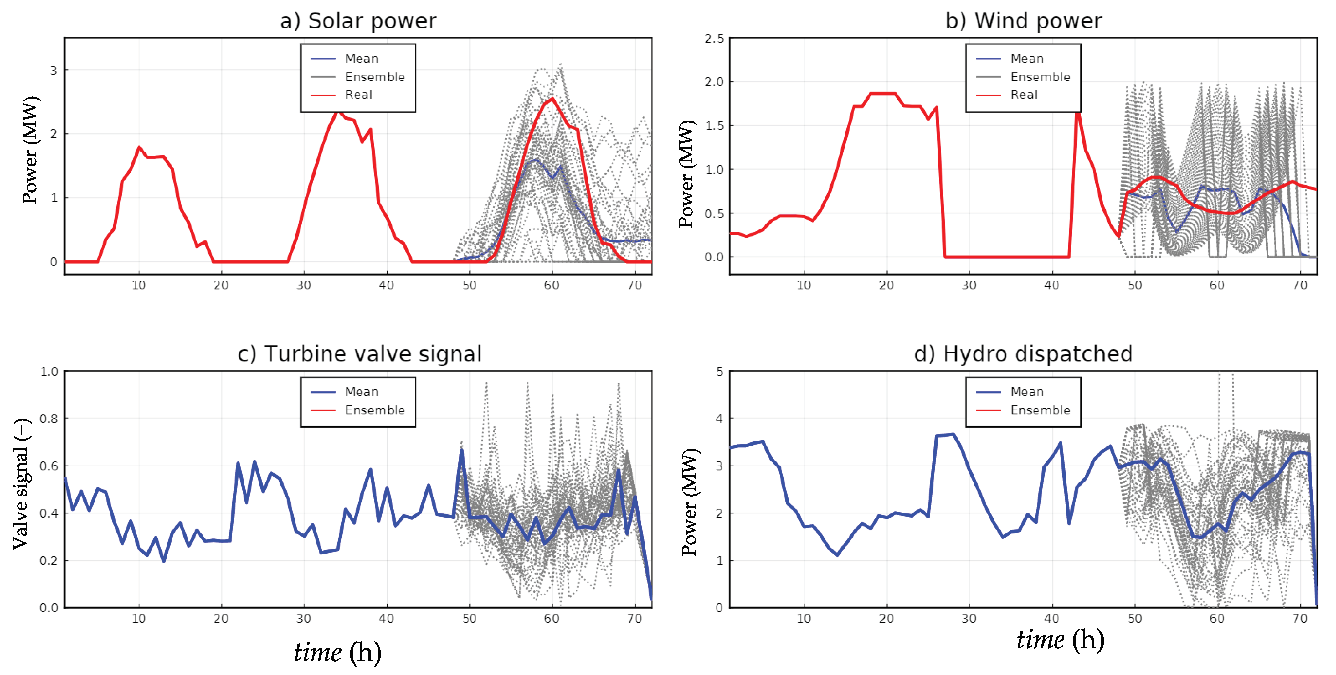
Figure 18a,b shows solar power and wind power based on solar irradiance and wind velocity as stochastic input to the microgrid. Figure 18c shows the turbine valve signal for the hydro-turbine.

Figure 18. Analysis of deterministic MPC with stochastic disturbances. For each of the scenarios, optimal control input solutions for $u_{\mathrm{v}}$ is found. The optimal control input of every scenarios is then plotted together.

6. Results and Discussion

From Figure 3 we saw that the grid frequency fluctuates with the injection of power into the grid. In addition, from Figure 4 with parameter sensitivity analysis we found that the grid frequency is the most sensitive state to the turbine valve signal rather than intermittent injection. Hence, the idea regarding the balancing load and generation should be primarily focused on increasing the rate of the turbine valve signal to cope up with the large variation of intermittent injection. This also supports the idea of flexible hydro power. Moreover, we also found that sensitivity in h and ${\dot{V}}_{\mathrm{s}}$ are periodic and oscillates over the solution. The sensitivity solution for ${\dot{V}}_{\mathrm{p}}$ due to the turbine valve signal $u_{\mathrm{v}}$ is exponentially decaying. The sensitivity solutions show the system oscillates. However, sensitivity in grid frequency $\omega$ due to $u_{\mathrm{v}}$ is exponentially rising, and crossing beyond the range of $\left(330\pm 5\%\right)\mathrm{rad}/\mathrm{s}$. This indicates that controller discretization time $\Delta t_{\mathrm{c}}$ should be chosen in such a way that grid frequency meets the constraints.

In a similar way, Figure 5 and Figure 6. show during power injection, the position of the turbine valve has an insignificant effect on the grid frequency fluctuation. The suitable discretization time for $6\mathrm{MW}$ reference load scheduling using solar power, wind power, and hydro power is found to be in the range $\left(1-10\right)\mathrm{s}$. Similarly, considering the inertia from hydro power plant as $J_{\mathrm{h}}=1\times {10}^3{\mathrm{kgm}}^2$ and wind power plant as $J_{\mathrm{w}}=0.1\times {10}^3{\mathrm{kgm}}^2$ we found that the maximum allowed controller discretization time is almost the same for both inertial and static power injection.

The grid frequency fluctuation increased as controller discretization time is higher as shown in Figure 8. The figure also shows that for a controller with a low $\Delta t_{\mathrm{c}}$ the response time of turbine valve signal increases. For models with and without process disturbance and measurement noise, Figure 12 shows that deviations in controlled signals are insignificant.

Figure 8. Grid frequency and turbine valve signal for different controller discretization time. The actual continuous solution of the turbine valve signal for specific discretization time is found using $time=\frac{k}{\Delta t_c}$ for $k\in [1,1000]$. Hence, readers should not compare results based on amplitude only.

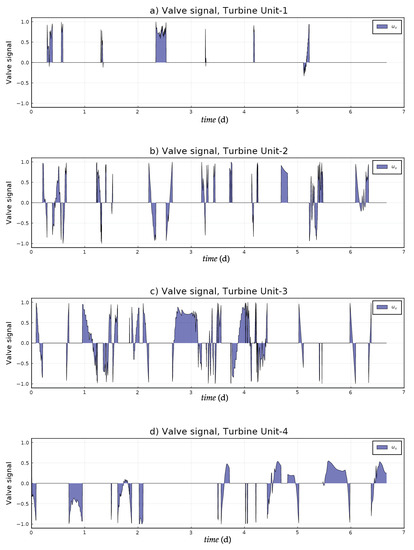
Figure 13 shows the hydro power plants operated in both motoring and generating mode. Turbine unit-1 is operated in generating mode, and throughout the day it is operated with a valve signal near unity. However, both turbine units 2 and 3 are operated in both generating and motoring mode, and the position of the valve signal is near unity. Turbine unit-3 is operated mostly in motoring mode with valve signal near unity. The valve signal $u_{\mathrm{v}}=0.5$ for unit-3 operating in generating mode. A rotating unit increases its efficiency based on loading. Hence, instead of considering a single unit, we tend to use four units of pump-turbine mostly to operate near full load i.e., near unity. Furthermore, units 2 and 3 are intermittently dispatching hydro power into the grid as both generating and motoring mode. Since we have considered $6\mathrm{MW}$ hydro power plant with four units each rated at $1.5\mathrm{MW}$, the intermittency in power productions from unit 2 and 3 can be removed by choosing units with different ratings. A particular choice for a rating of the unit depends on solar irradiance, wind velocity, and schedule load at a particular location. The choice is made mostly by analyzing the yearly hydro schedule dispatched into the grid for balancing load and generations. Since both solar and wind power productions are stochastic we tend to perform yearly scheduling based on the stochastic analysis.

The future prediction of solar power, wind power, and scheduled load are performed formulating a state-space model. Similarly, we can also perform the future prediction of solar and schedule load based on confined space for Weibull and normal distribution using relaxation parameters. The confined space from Weibull and normal distributions provides a continuously differentiable function for running a continuous-time model. Furthermore, scenario analysis for the predicted solar power, wind power, and schedule load is done in two ways, using Monte Carlo simulation and 95 % confidence interval.

Figure 14 shows yearly parameter space for solar irradiance prediction using both a Weibull and normal distribution. The average yearly parameter space is generated by analyzing past yearly parameter spaces. The account of shadowing throughout the day is not considered while modeling with the Weibull and normal distribution. The parameters are found in such a way that the effect of the shadow is averaged out using least-squares data fit for a particular day. This implies that the prediction is based on the average solar irradiance on a sunny day throughout the year. Figure 15 shows the solar irradiance prediction using both Weibull and normal distributions. Based on the RMSE errors, the normal distribution is better for solar irradiance prediction rather than the Weibull distribution. The relaxation parameter $\alpha$ for the Weibull distribution as in Figure 14 shows that sliding over the negative space is not possible; however possible for the normal distribution. Hence, the normal distribution is better for solar irradiance prediction. A more rigorous prediction algorithm can be developed to study the effect of shadowing in the parameter space of the Weibull or normal distribution. A simple idea would be to inject the information of shadow in between the confined space, like $[\alpha ,\beta ]=[\alpha ,s_1)\cup [s_1,s_2)\cup [s_2,\beta ]$ where $s_1$ and $s_2$ are starting and ending of the shadowing event, respectively.

The prediction of load demand as shown in Figure 17b using a state-space model is performed based on different seasonality in a year, a month, and a day or an hour. The hourly prediction can be improved based on a prediction from monthly to weekly to daily rather than the prediction from only the past few days. The result shows that scenarios are generated better with Monte Carlo methods than using the confidence intervals. However, scenarios generated from confidence intervals are computationally cheap is used for hydro scheduling analysis; this adheres to computationally cheap solutions for studying flexible hydro powers. Figure 18c,d show mean and ensemble turbine valve signal and hydro dispatched into the grid for different scenarios inputs from solar power, wind power, and schedule load. From Figure 17b–d, the range of deviations in scenarios for control input $u_{\mathrm{v}}$ and hydro dispatched $P_{\mathrm{h}}$ increases when $v_{\mathrm{w}}>7\mathrm{m}/\mathrm{s}$ because of shutdown of wind turbine where $P_{\mathrm{w}}=0.$ Figure 18 shows inputs and outputs result from the first 3 days in the month of July 2018. The first two days results are from deterministic MPC while the last day results are from the stochastic analysis of deterministic MPC.

7. Conclusions

This paper explores the possibility of using MPC to balance intermittent generations from solar and wind power using dispatchable hydro powers. We found that grid frequency can be controlled within a required range of limits using the best controller discretization time. The controller discretization time for running an optimal control problem inside MPC is found using maximum allowed discretization time to maintain the grid frequency. The maximum allowed discretization time is found analyzing injection of intermittent generation into the grid at a different sampling rate of solar power, wind power, and consumer load. The discretization time for the controller of a microgrid with a consumer load capacity of $6\mathrm{MW}$ with solar power, wind power, and hydro power in the range of $\left(2-4\right)\mathrm{MW}$ is found to be $10\mathrm{s}$. We also found that the position of the valve during static power injection into the grid has an insignificant effect on the grid frequency fluctuation and the choice of discretization time for the controller. We could not conclude about the relations between discretization time for controller and inertial power injection into the grid.

8. Future Work

Future work includes the study of a dynamical model of a microgrid with constraints on both voltage level and grid frequency. The effect of inertial injection from the wind power plant can be studied with dynamic equations of wind power plants. Wind turbines are shut down when the velocity of wind is beyond the operational limit of wind turbines. This will cause the wind turbines out of their rotational limit, and the inertial effect of the wind turbines into the grid is detached from the overall grid inertia. The effect of inertial injection into the grid can be studied with dynamic equations considering detaching of wind turbines when the wind velocity crosses the permitted limit.

References

- Charmasson, J.; Belsnes, M.; Andersen, O.; Eloranta, A.; Graabak, I.; Korpås, M.; Helland, I.; Sundt, H.; Wolfgang, O. Roadmap for Large-Scale Balancing and Energy Storage from Norwegian Hydropower: Opportunities, Challanges and Needs until 2050; Opportunities, Challenges and Needs Until; SINTEF Energi AS: Trondheim, Norway, 2018. [Google Scholar]
- Graabak, I.; Jaehnert, S.; Korpås, M.; Mo, B. Norway as a battery for the future european power system—impacts on the hydropower system. Energies 2017, 10, 2054. [Google Scholar] [CrossRef] [Scilit]
- Graabak, I.; Korpås, M.; Jaehnert, S.; Belsnes, M. Balancing future variable wind and solar power production in Central-West Europe with Norwegian hydropower. Energy 2019, 168, 870–882. [Google Scholar] [CrossRef] [Scilit]
- Graabak, I.; Korpås, M. Balancing of variable wind and solar production in Continental Europe with Nordic hydropower–A review of simulation studies. Energy Procedia 2016, 87, 91–99. [Google Scholar] [CrossRef] [Scilit]
- Steen, D.; Goop, J.; Göransson, L.; Nursbo, S.; Brolin, M. Challenges of integrating solar and wind into the electricity grid. Systems Perspectives on Renewable Power; Chalmers University of Technology: Gothenburg, Sweden, 2014; pp. 94–107. [Google Scholar]
- Ahmed, S.D.; Al-Ismail, F.S.; Shafiullah, M.; Al-Sulaiman, F.A.; El-Amin, I.M. Grid integration challenges of wind energy: A review. IEEE Access 2020, 8, 10857–10878. [Google Scholar] [CrossRef] [Scilit]
- Zhou, W. Modeling, Control and Optimization of a Hydropower Plant; University College of Southeast Norway: Notodden, Norway, 2017. [Google Scholar]
- Liu, X.; Zhang, Y.; Lee, K.Y. Coordinated distributed MPC for load frequency control of power system with wind farms. IEEE Trans. Ind. Electron. 2016, 64, 5140–5150. [Google Scholar] [CrossRef] [Scilit]
- Liu, X.; Zhang, Y.; Lee, K.Y. Robust distributed MPC for load frequency control of uncertain power systems. Control. Eng. Pract. 2016, 56, 136–147. [Google Scholar] [CrossRef] [Scilit]
- Munoz-Hernandez, G.A.; Jones, D.I. Modelling and Controlling Hydropower Plants; Springer Science & Business Media: Berlin/Heidelberg, Germany, 2012. [Google Scholar]
- Flórez, J.Z.; Martinez, J.J.; Besançon, G.; Faille, D. Explicit coordination for MPC-based distributed control with application to Hydro-Power Valleys. In Proceedings of the 2011 50th IEEE Conference on Decision and Control and European Control Conference, Orlando, FL, USA, 12–15 December 2011; pp. 830–835. [Google Scholar]
- Magdy, G.; Shabib, G.; Elbaset, A.A.; Mitani, Y. Frequency stabilization of renewable power systems based on mpc with application to the egyptian grid. IFAC-PapersOnLine 2018, 51, 280–285. [Google Scholar] [CrossRef] [Scilit]
- Avramiotis-Falireas, I.; Troupakis, A.; Abbaspourtorbati, F.; Zima, M. An MPC strategy for automatic generation control with consideration of deterministic power imbalances. In Proceedings of the 2013 IREP Symposium Bulk Power System Dynamics and Control-IX Optimization, Security and Control of the Emerging Power Grid, Rethymnon, Crete, Greece, 25–30 August 2013; pp. 1–8. [Google Scholar]
- Bhagdev, D.; Mandal, R.; Chatterjee, K. Study and application of MPC for AGC of two area interconnected thermal-hydro-wind system. In Proceedings of the 2019 Innovations in Power and Advanced Computing Technologies (i-PACT), Vellore, India, 22–23 March 2019; Volume 1, pp. 1–6. [Google Scholar]
- Reigstad, T.I.; Uhlen, K. Optimized Control of Variable Speed Hydropower for Provision of Fast Frequency Reserves. Electr. Power Syst. Res. 2020, 189, 106668. [Google Scholar] [CrossRef] [Scilit]
- Welcome to OpenModelica-OpenModelica. OpenModelica. Available online: https://www.openmodelica.org/ (accessed on 12 May 2020).
- Modelica Association. The Modelica Association-Modelica Association. Available online: https://www.modelica.org/ (accessed on 12 May 2020).
- Pandey, M.; Lie, B. The Role of Hydropower Simulation in Smart Energy Systems. In Proceedings of the 2020 IEEE 7th International Conference on Energy Smart Systems (ESS), Kyiv, Ukraine, 12–14 May 2020; pp. 392–397. [Google Scholar]
- University of South-Eastern Norway. OpenHPL-Home. Available online: https://openhpl.simulati.no (accessed on 12 May 2020).
- Rensselaer Polytechnic Institute, ALSETLab. OpenIPSL’s documentation!-OpenIPSL 1.0.0 documentation. Available online: https://openipsl.org (accessed on 12 May 2020).
- Pearson, R. PhotoVoltaics. Available online: https://raulrpearson.github.io/PhotoVoltaics/ (accessed on 12 May 2020).
- Kral, C. WindPowerPlants|Dr. Christian Kral. Available online: http://www.christiankral.net/en/modelica/windpowerplants (accessed on 12 May 2020).
- JuliaLang.org contributors. The Julia Programming Language. Available online: https://julialang.org/ (accessed on 12 May 2020).
- Dunning, I.; Huchette, J.; Lubin, M. JuMP: A Modeling Language for Mathematical Optimization. SIAM Rev. 2017, 59, 295–320. [Google Scholar] [CrossRef] [Scilit]
- Revels, J.; Lubin, M.; Papamarkou, T. Forward-Mode Automatic Differentiation in Julia. arXiv 2016, arXiv:1607.07892 [cs.MS]. [Google Scholar]
- Open Source Modelica Consortium. OMJulia–OpenModelica Julia Scripting. Available online: https://https://www.openmodelica.org/doc/OpenModelicaUsersGuide/latest/omjulia.html (accessed on 12 May 2020).
- Saavedra, R.; Bodin, G.; Souto, M. StateSpaceModels.jl: A Julia Package for Time-Series Analysis in a State-Space Framework. arXiv 2019, arXiv:1908.01757. [Google Scholar]
Publisher’s Note: MDPI stays neutral with regard to jurisdictional claims in published maps and institutional affiliations. |
© 2021 by the authors. Licensee MDPI, Basel, Switzerland. This article is an open access article distributed under the terms and conditions of the Creative Commons Attribution (CC BY) license (http://creativecommons.org/licenses/by/4.0/).