Restoration of Missing Pressures in a Gas Well Using Recurrent Neural Networks with Long Short-Term Memory Cells

Abstract

This study proposes a data-driven method based on recurrent neural networks (RNNs) with long short-term memory (LSTM) cells for restoring missing pressure data from a gas production well. Pressure data recorded by gauges installed at the bottom hole and wellhead of a production well often contain abnormal or missing values as a result of gauge malfunctions, noise, outliers, and operational instability. RNNs employing LSTM cells to prevent long-term memory loss have been widely used to predict time series data. In this study, an RNN with the LSTM method was used to restore abnormal or missing wellhead and bottom-hole pressures in three intervals within a production sequence of more than eight years in duration. The pressure restoration was performed using various input features for RNNs with LSTM models based on the characteristics of the available data. It was carried out through three sequential processes and the results were acceptable with a mean absolute percentage error no more than 5.18%. The reliability of the proposed method was verified through a comparison with the results of a physical model.

1. Introduction

Production rates and flowing pressures in oil/gas production wells are essential information for planning field development and reservoir management to maximize recovery. Multiphase flow meters can enable production rates to be measured in real time [1]; however, in reality, owing to the high cost of flow meters, the common practice is to apply a back-allocation methodology based on the field total production measured through the high-pressure separator that connects all the production wells [2]. This back-allocation method is commonly carried out based on the periodic measurements of the test separator that measures the production rate of each well.

The tubing head pressure (THP) and bottom-hole pressure (BHP) are measured in real time using gauges installed at the wellhead and bottom-hole sites, respectively. However, some pressure data are missing or exhibit abnormal peaks, errors, or noise due to the intermittent malfunctioning of the gauges during long-term operation [3]. In addition, abnormal data can be acquired during periodic maintenance work at the production wells or with the replacement of relevant equipment due to on-site safety issues. To use the measured field data in decision-making for reservoir management, the dataset should be preprocessed through data cleaning, conditioning, and filtering [4]. Data quality control can be performed using advanced techniques such as reservoir simulations or well modeling. However, sufficient expertise and analysis is required for these methods, which also require a large amount of time and effort.

To restore missing or contaminated data, machine learning methods can be utilized. Machine learning methods infer the relationship between the input and output data of a system, rather than analyzing the inherent physical principles of the system theoretically or numerically [5]. Recently, machine learning techniques have been widely applied in the exploration and production industry. Previous studies that incorporated machine learning methods have focused on a decline curve analysis and estimated the ultimate recovery prediction in shale gas reservoirs [6,7,8], automatic detection of events during drilling campaigns [9,10], drilling location optimization [11,12,13,14], and inverse modeling based on the production history [15,16].

Machine learning techniques have also been utilized for fluid flow modeling in production wells. An artificial neural network (ANN) technique was applied to analyze the pressure drops in vertical wells, and the performance of the ANN-based model was comparable to the results of the conventional method using existing empirical correlations with the actual pressure drop measurements [17]. Several attempts have been made to improve the accuracy of pressure predictions; some have modified the structure of the ANN model, while others have varied the optimization algorithms [18,19]. Recently, a deep neural network (DNN) model was proposed for BHP prediction in multiphase production wells [20]. Even though the neural network structure in the model is relatively simple with three input features (THP, flow rate, and well schematics) and just two hidden layers, the model showed a good prediction performance under various flow conditions.

Recurrent neural networks (RNNs) are a type of DNN technique that are specialized for analyzing time series data [21]. However, they have a limitation in that the training efficiency becomes poor with more hidden layers or a longer time series. To overcome this problem, long short-term memory (LSTM) cells have been introduced to RNNs [21,22], and their applicability has been validated by several studies. The RNN method with LSTM cells was applied in production forecasts for shale gas reservoirs [23] and estimations of the production capacity by learning time series data for the BHP and bottom-hole temperature [24]. Recently, the restoration of missing THP data in a gas well was performed using the RNN method with LSTM cells [25], where the THP, BHP, and gas flow rate data were used for input features. The reliability of the result was validated by a comparison with the result from the physics-based model.

In this study, an RNN with an LSTM technique is applied to restore missing parts of the THP and BHP time series in production data for a gas field collected over more than eight years. The restoration processes are based on the previous study [25] and further improved to consider complicated circumstances. Various features are considered for the data-driven model based on the available data characteristics in the entire period, and a concept of equivalent gas production is introduced to include the effect of the late-time water production. The results are validated by a comparison with the conventional model-based results.

2. Materials and Methods

2.1. Target Well Data

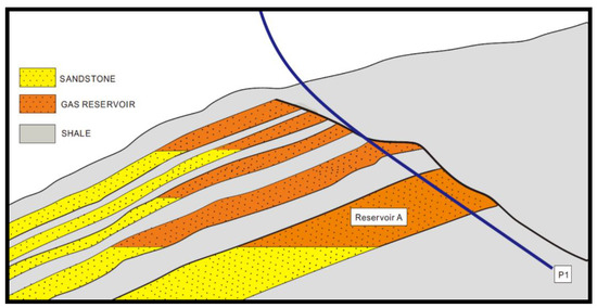
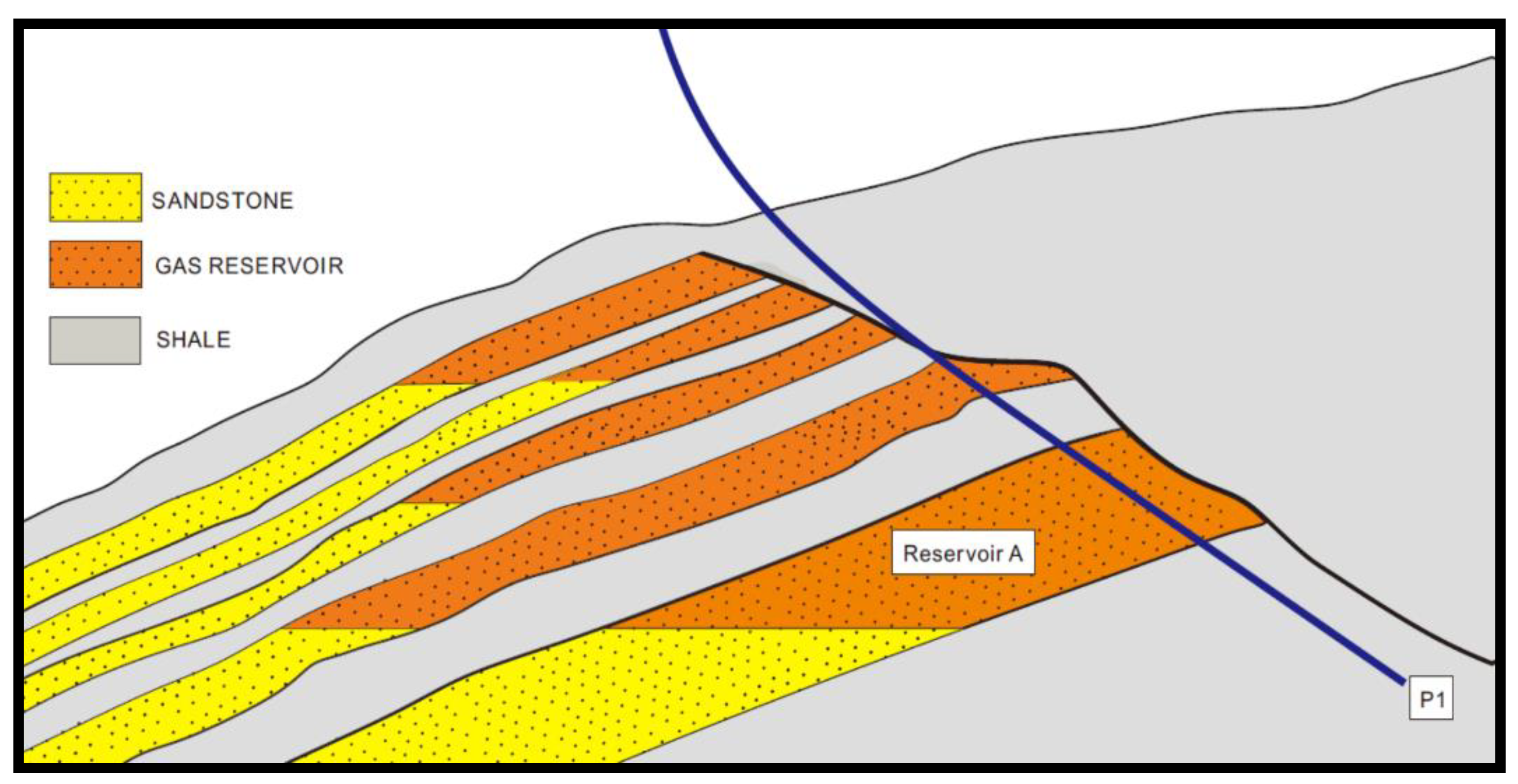
Figure 1 shows an offshore gas field with a target well, P1, in this study. The reservoir information such as the location of the field, the reservoir depth, and reservoir properties cannot be revealed for commercial reasons. It has been producing gas and condensate from the lowest formation (Reservoir A) for more than eight years. The existence of an aquifer was confirmed through the modular formation dynamics test data acquired from an exploration well, which may cause water issues in the formation. In fact, there was no formation water production in the early stages of operation; however, lately, the well has been producing formation water with decreased gas production. When a gas well begins to flow after being shut-in for various reasons, liquid loading at the bottom of the tubing is likely to occur in a lowered reservoir pressure. Therefore, the production performance of the gas well should be closely monitored through the BHP and THP trends along with the flow rate information. In addition, during a long-term shut-in period for regular maintenance, water intrusion to the near-wellbore formation may occur, resulting in productivity loss or no gas production upon the subsequent re-opening of the well. This necessitates additional time-consuming and expensive solutions, such as the injection of methanol or hydrocarbon gas, to restore the well productivity.

Figure 1. Schematic diagram of the gas reservoir with a target well (modified from Korea National Oil Corporation (KNOC) [26]).

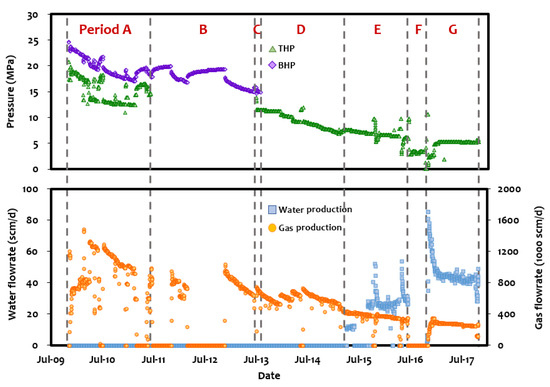
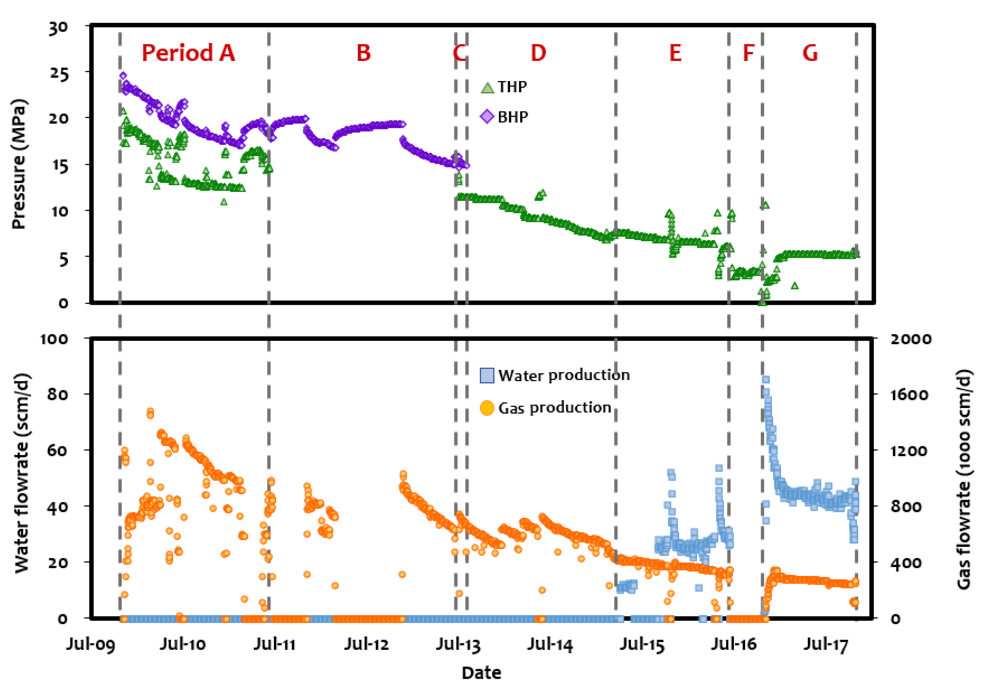
Figure 2 shows the production profile of the gas and water flow rates, BHP, and THP in the target well over approximately eight years. The target well has been operated by adjusting the choke value in accordance with field-scale operational issues and management plans. The whole production interval is divided into seven periods (Periods A to G) based on the data acquisition status and production performance, as shown in Figure 2. The daily gas and water flow rates were back-allocated based on the separator measurement, while the flow pressures were recorded by gauges at midnight each day. It should be noted that the well started water production from Period E.

Figure 2. Production profile of the target well (scm: standard cubic meters).

Table 1 summarizes the acquired dataset for each period in Figure 2. The condensate–gas ratio (CGR) was nearly constant at $1.35\times {10}^{-4}$ scm oil/scm gas over the entire period (scm stands for cubic meters at the standard condition, where the standard condition refers to 15.56 °C and 101.3 kPa). Period A has datasets for the BHP, THP, and the gas flow rate; the THP was maintained above 12.4 MPa as the minimal flow condition, and the gas flow rate decreased accordingly. The well operation was complex, with frequent changes in the choke size. Period B comprises two sets of the long-term shut-in and flowing sequences; only the datasets for BHP and gas flow rate are available owing to a malfunction of the wellhead gauge.

Table 1. Summary of data acquisition.

Period	Days	Data Acquisition	Remarks
A	581	Qg 1, Qcon 2, BHP, THP
B	751	Qg, Qcon, BHP	simple operation (2 BUs and DDs) no THP data
C	31	Qg, Qcon, BHP, THP
D	612	Qg, Qcon, THP	no BHP data
E	439	Qg, Qcon, Qwater 3, THP	commencement of water production no BHP data
F	142	Qg, Qcon, Qwater, THP	shut-in no BHP data, abnormal THP data
G	360	Qg, Qcon, Qwater, THP	liquid loading gas productivity recovered

¹ Daily gas production, ² daily condensate production, ³ daily water production.

Because the gauge at the wellhead was repaired before Period C, datasets for the BHP, THP, and gas flow rate were available for one month in Period C. Then, the bottom-hole gauge malfunctioned; thus, there is no BHP data available for Periods D to G. In Period E, the production of formation water commenced, which caused the gas productivity to decrease and the pressure drop through the tubing to increase gradually; however, it was not feasible to analyze these phenomena properly owing to the absence of BHP data.

Period F was a shut-in period for regular maintenance work, and only THP data were available. However, the pressure data exhibited erroneous behavior in which the pressure values were lower than those in the previous flowing period. During the shut-in of Period F, a mixture of three phases, i.e., gas, condensate, and water, was segregated by gravity through the tubing. Then, the water in the bottom-hole part of the tubing was expected to intrude into the reservoir and hinder gas from flowing into the tubing in the subsequent period. This phenomenon was confirmed by the subsequent flowing period (Period G). The water production in Period G started with an extremely high value in comparison with the production level in Period E and decreased rapidly. The gas flow rate exhibited the reverse behavior: the gas production was recovered from the very low rate in the early part of Period G, and then followed the trend of global decline observed in Period E. Therefore, the decreased productivity of gas in the wellbore region due to water intrusion seems to be recovered after the early part of Period G. The THP also increased from low values at the beginning of Period G due to the excessive water production and recovered a similar declining trend as that observed in Period E.

2.2. RNN

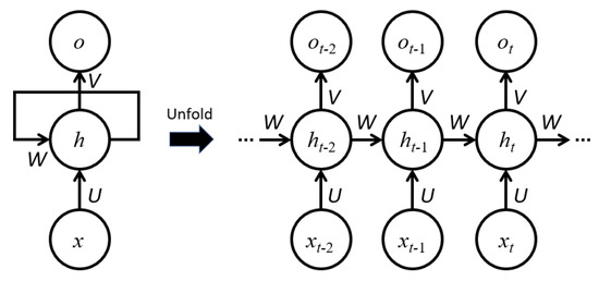
RNN models have been widely used for time series data analyses such as stock price prediction, voice recognition, and automatic translation [21]. While information flows in one direction from the input node to the output node through hidden nodes in a conventional neural network, information can flow recursively though hidden nodes with time in an RNN system. Figure 3 shows the basic structure of the RNN system, where $x$, $h$, and $o$ represent the input layer, hidden layer, and output layer, respectively; $U$ and $V$ are the weights of the connections between the input and hidden layers and between the hidden and output layers, respectively; $W$ represents the weight of the connection between the hidden layers at the current time and the next time as the time series input data were injected continuously.

Figure 3. Structure of the recurrent neural network (RNN).

The right side of Figure 3 shows the circulation structure, explaining its recurrent scheme for sequential time series data; the left side of Figure 3 shows the unfolding of the recurrent structure of the hidden layer. The principle of RNNs is as follows: when the value of $x_{t-1}$ at time t-1 is injected, the hidden layer value, $h_{t-1}$, is determined by combining with the hidden layer value of $h_{t-2}$ transferred from the previous time (t-2). This hidden layer value is passed to the output layer and is also transferred recurrently to the hidden layer at the next time (t). Therefore, the RNN is designed such that past data in the time series affect the future by passing information from the previous time to the next time through the hidden layer. Equations (1) and (2) summarize the process.

$$h_t=f\left(U{x}_t+W{h}_{t-1}+b\right)$$

(1)

$$o_t=g\left(V{h}_t+c\right)$$

(2)

where $x_t$, $h_t$, and $o_t$ are the values of the input, hidden, and output layers, respectively; $U$, $W$, and $V$ represent weights between adjacent layers; $f$ and $g$ represent activation functions at the hidden and output layers, respectively; b and c indicate biases, which are constant.

2.3. LSTM

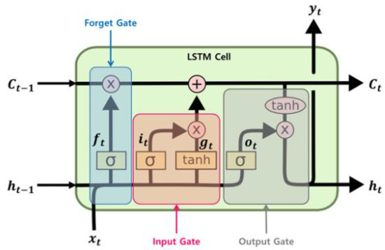
The RNN method specializes in forecasting future performance by training the model with past time series data. However, when the length of the time series in the training data increased, the information for the early times had a lesser influence on forecasting than the information for the later times, which is known as the gradient vanishing problem in DNNs. To overcome this problem of disappearing long-term memory dependency, the LSTM cell technique has been proposed [22]. Figure 4 shows the structure of the LSTM cell, which can be used as a replacement for the nodes in the hidden layers of the RNN shown in Figure 3. The LSTM cell has a short-term state, $h_t$, and a long-term state, $C_t$, delivered to the next time point. The long-term memory is preserved by $C_t$, thus allowing the problem of disappearing long-term memory dependency to be solved.

Figure 4. Long short-term memory (LSTM) cell structure [27].

There are three gates in the LSTM internal structure, i.e., the forget, input, and output gates, as shown in Figure 4. The role of the forget gate is to delete unnecessary information from the long-term memory. Then, the necessary information is stored in long-term memory through the input gate. The output gate determines the short-term memory to be transferred to the next time point. The LSTM process is described by Equations (3)–(8).

$$f_t=\sigma \left(U_f{x}_t+W_f{h}_{t-1}+b_f\right)$$

(3)

$$i_t=\sigma \left(U_i{x}_t+W_i{h}_{t-1}+b_i\right)$$

(4)

$$o_t=\sigma \left(U_o{x}_t+W_o{h}_{t-1}+b_o\right)$$

(5)

$$g_t=\sigma \left(U_g{x}_t+W_g{h}_{t-1}+b_g\right)$$

(6)

$$C_t=f_t\otimes C_{t-1}+i_t\otimes g_t$$

(7)

$$h_t=o_t\otimes tanh\left(C_t\right)$$

(8)

where $f_t$, $i_t$, and $o_t$ represent the values of the forget gate, input gate, and output gate, respectively; $g_t$ analyzes the current information and delivers it to the long-term state; $U_f$, $U_i$, $U_o$, and $U_g$ are the weights of the gates in connection with the input value ($x_t$); $W_f$, $W_i$, $W_o$, and $W_g$ represent the weights in connection with $h_{t-1}$, which is the short-term state at the previous time (t-1); $b_f$, $b_i$, $b_o$, and $b_g$ are constants representing the biases at the gates; $\sigma$ represents the sigmoid function used as the activation function; $\otimes$ denotes elementwise multiplication.

2.4. Verification with the Physical Model

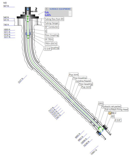
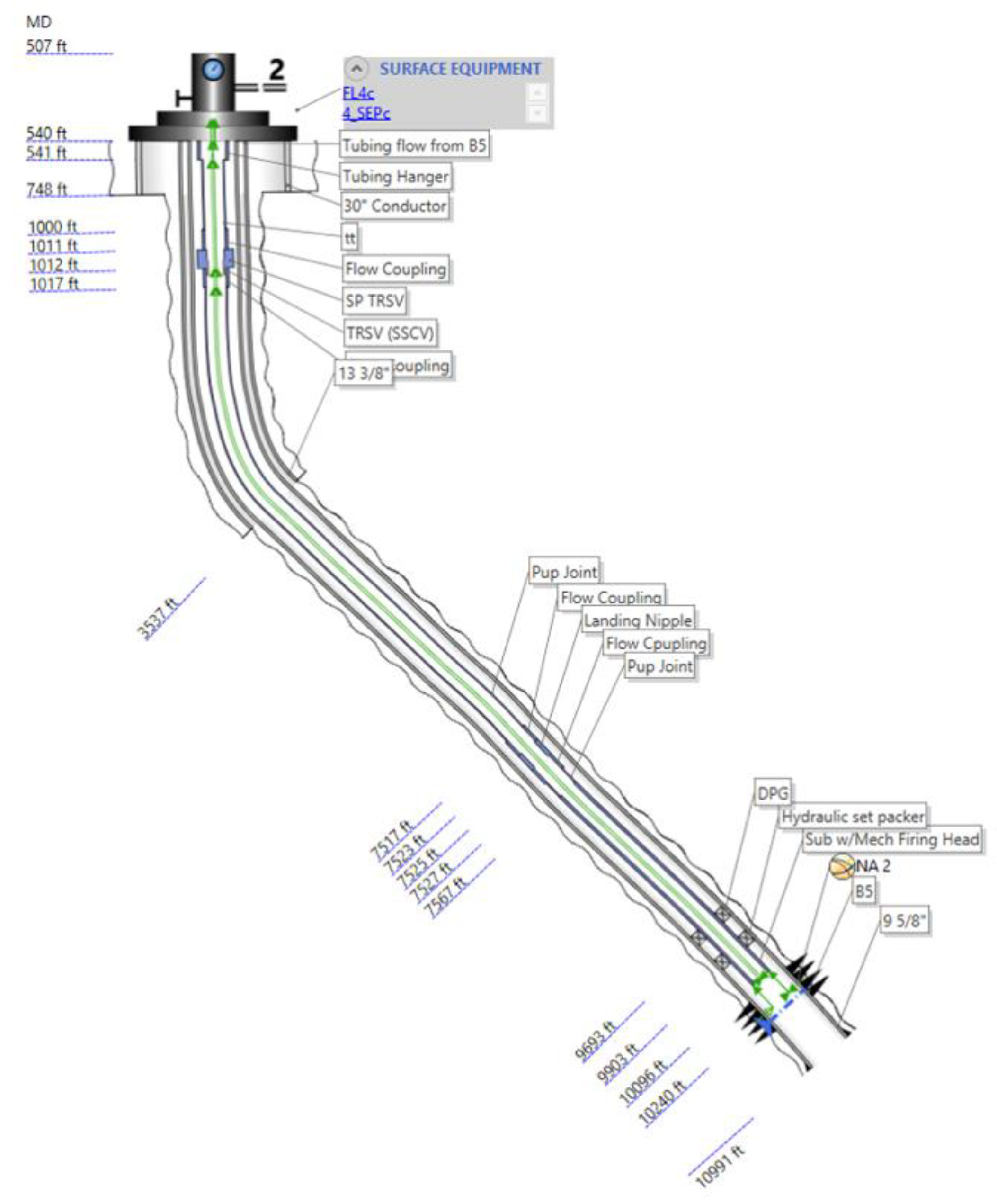
The pressure data predicted using the RNN model with LSTM cells (hereinafter referred to as RNN-LSTM) in this study were verified using PIPESIM software, which is a steady-state multiphase flow simulator for production wells [28]. PIPESIM can be used to construct the structure of the production well and investigate the relationship among the production rate, THP, and BHP by solving the physics-based governing equation. The pressure predictions obtained with the RNN-LSTM model were compared with the results obtained using PIPESIM. Figure 5 shows a schematic of the target well used in the PIPESIM model with the Begg and Brill correlation [29].

Figure 5. Target well schematic for the PIPESIM model.

3. Results and Discussion

3.1. Processes for Restoring the Missing Pressures

Because the reservoir pressure decreased throughout the production period in Figure 2, it is important to estimate the future productivity of the well. To understand the future performance and estimate the reserves, it is necessary to restore the missing or erroneous BHP and THP data. In this study, data restoration was performed using the RNN-LSTM method through the following three processes:

• Process 1: THP prediction in Period B,
• Process 2: THP prediction in Period F,
• Process 3: BHP prediction in Periods D, E, F, and G.

Process 1 has been performed by a previous study [25] using the RNN-LSTM methodology, where an RNN model was constructed to predict the THP for Period B. After THP, BHP, and gas production data from Period A were used to train the RNN-LSTM model, the THP for Period B was estimated. The results are summarized in the following section.

Process 2 predicts the THP for the buildup in Period F. Because there are no BHP data for Periods D to G, only the THP and gas production data were used for training the RNN-LSTM model. In this case, the restored THP data for Period B obtained in Process 1 are used as input data. In Process 3, data restored from Processes 1 and 2 were used to train the RNN-LSTM model to predict the BHP data for Periods D to G.

The prediction processes for the THP of Period B (Process 1) and BHP of Periods D to G (Process 3) seem to be similar, but there are some differences. To predict the THP of Period B, the BHP and THP data of Period A were learned by the RNN-LSTM model. Period B is composed of two sets of the long-term shut-in and flowing sequences, and except for the last flowing period, the BHP pressures in Period B are within the range of BHP values obtained in Period A. The THP seems to have the same situation. Therefore, the RNN-LSTM model trained using the data from Period A can be expected to have a good predictive performance for the pressure in Period B.

On the other hand, we consider the case where the RNN-LSTM is trained using the pressure data from Periods A to C to predict the BHP of Periods D to G (Process 3). Periods D to G consist of lower THP values than those in Periods A and B. In other words, the RNN-LSTM model trained using the data from Periods A to C needs to predict BHP values beyond the range of the data used for the training. Thus, it is very possible that the predictive performance will deteriorate. Process 2 has a similar situation, in that the THP prediction in Period F uses production data obtained for a very long time before Period F. Thus, long-term decreasing pressure data should be used as the input feature, which may also degrade the performance of the RNN-LSTM model. To compensate for these degradations in Processes 2 and 3, the RNN-LSTM models require different input variables from those used in Process 1. Thus, Process 2 introduces the pressure difference between two adjacent values in THP data, and Process 3 introduces the pressure difference between the THP and BHP values of the same time. In this way, the values of the pressure difference in the prediction periods are expected to be within the range of those in the training data, which can circumvent the aforementioned degradation problems. In addition, Processes 2 and 3 introduce the cumulative gas production as an input feature to partially consider the effect of the long-term decrease in reservoir pressure due to gas production.

3.2. Setup of the RNN-LSTM Model

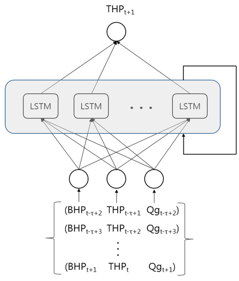
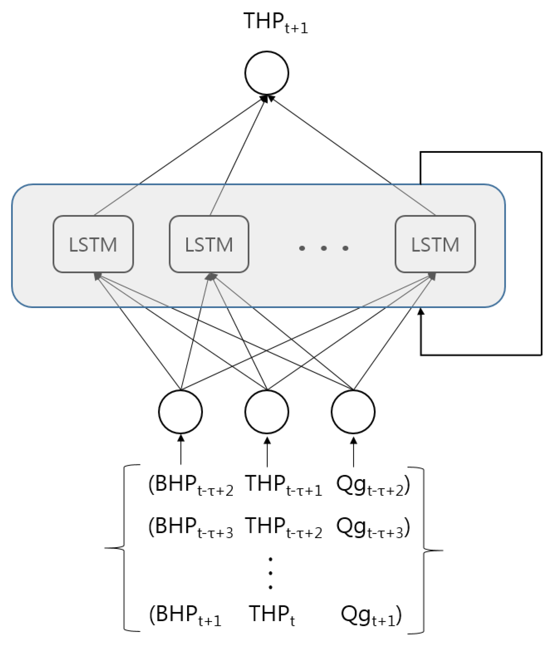
Figure 6 shows an example of the RNN-LSTM models constructed in this study. The system predicts the output variable at the (t + 1) th time step using an input sequence with a length of τ backward from the tth time step. The output variable at the (t + 1) th time step may be directly affected by the input variable at the same time step. Therefore, any input variables other than the target variable, if available, at the (t + 1) th time step can also be used as input features. For example, consider that an RNN-LSTM model predicts the THP at the (t + 1) th time step using a sequence with a length of τ composed of THP, BHP, and Qg data. Then, it can be conjectured that the THP at the (t + 1) th time step will be affected by the BHP and gas rate at the same time step, and thus the input data can be constructed in the form of {(THP_t-τ+1, BHP_t-τ+2, Qg_t-τ+2), (THP_t-τ+2, BHP_t-τ+3, Qg_t-τ+3), …, (THP_t, BHP_t+1, Qg_{t +1})} to predict THP_t+1.

Figure 6. Example of the RNN-LSTM models in this study.

Table 2 lists the hyperparameters applied in Processes 1 to 3. Different types of available data and validation schemes for each process allow the hyperparameters to be customized, as presented in Table 2. Process 1 has three input features, i.e., THP, BHP, and Qg, and one output variable, while Process 2 has four input features, i.e., THP, the pressure difference between adjacent THPs, Qg, and the cumulative gas production. Process 3 has different input features from Process 1 because the pressures are beyond the range of the training data from Periods A to C. Therefore, the input features in Process 3 are composed of THP, Qg, the cumulative gas production, and the difference between THP and BHP. Moreover, rather than BHP, the output variable was also set to the pressure difference between THP and BHP.

Table 2. Hyperparameters of the RNN-LSTM methods for the three processes.

Hyper-Parameter	Process 1	Process 2	Process 3
Prediction purpose	THP in Period B	THP in Period F	BHP in Periods D, E, F, and G
Dataset	Daily data	Weekly data	Weekly data
Input features	THP, BHP, Qg	THP, △P (= THPt − THPt-1), Qg, Cumulative gas	THP, △P (= BHP − THP), Qg, Cumulative gas
Output target	THP	△P (= THPt+1 − THPt)	△P (= BHP − THP)
Length of input sequence (τ)	300	180	100
Input node	3	4	4
Hidden nodes (LSTM cells)	100
Output nodes	1
Optimization algorithm	Adam
Loss function	MAE
Epoch	300

All of the available data were normalized using Equation (9). Thus, all of the data have values between 0 and 1.

$$x_{norm}=\frac{x-x_{min}}{x_{max}-x_{min}}$$

(9)

where $x$ is the original value, and $x_{norm}$ represents the normalized value of $x$; $x_{max}$ and $x_{min}$ indicate the maximum and minimum values, respectively.

As loss functions, which are a measure of optimization, the mean absolute error (MAE) and mean absolute percentage error (MAPE) shown in Equations (10) and (11) are used. After a sufficient number of epochs is applied for training, the optimized model that can estimate the missing variables with the lowest error based on the validation data during the training process is selected.

$$\mathrm{MAE}=\frac{1}{n}{\displaystyle \sum }_{i=1}^n|O_i{}^{true}-O_i{}^{pred}|$$

(10)

$$\mathrm{MAPE}=\frac{100}{n}{\displaystyle \sum }_{i=1}^n\left|\frac{O_i{}^{true}-O_i{}^{pred}}{O_i{}^{true}}\right|$$

(11)

where $O_i{}^{true}$ and $O_i{}^{pred}$ represent the true and predicted values from the model, respectively, and n is the number of training data. One hidden layer with 100 LSTM cells was employed, and Adam was used as an optimization algorithm. Python with Tensorflow-Keras [30] was used to implement the RNN-LSTM method.

3.3. Process 1: THP Prediction during Period B

As mentioned in the previous section, Process 1 was carried out in the previous study [25], and the main results are summarized as follows. The input data are composed of a set of THP, BHP, and Qg from Period A using Equation (12), and the output is the THP at the $\left(t+1\right)$th time step given in Equation (13). The number of time steps in the input data sequence is $\tau$: BHP and Qg use data from the ($t-\tau +1)$th to ($t+1)$th time steps, while THP uses data from the ($t-\tau$)th to $t$th time steps. Note that the BHP and Qg at the ($t+1$)th time step are used to predict the THP value at the ($t+1$)th time step, which results in a more accurate and reliable model.

$$\mathrm{Input}=\left\{\left({\mathrm{THP}}_{t-\tau +i},{\mathrm{BHP}}_{t-\tau +i+1},{\mathrm{Qg}}_{t-\tau +i+1}\right)\right|1\le i\le \tau \}$$

(12)

$$\mathrm{Output}={\mathrm{THP}}_{t+1}$$

(13)

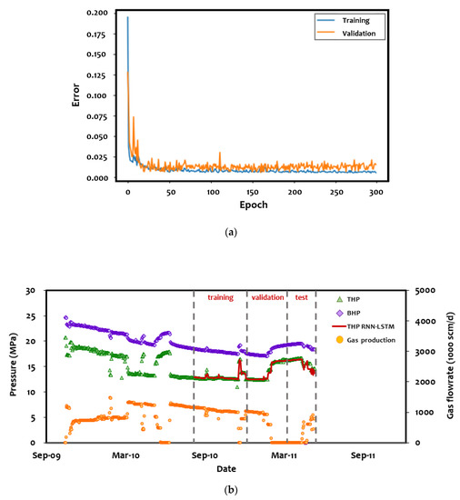
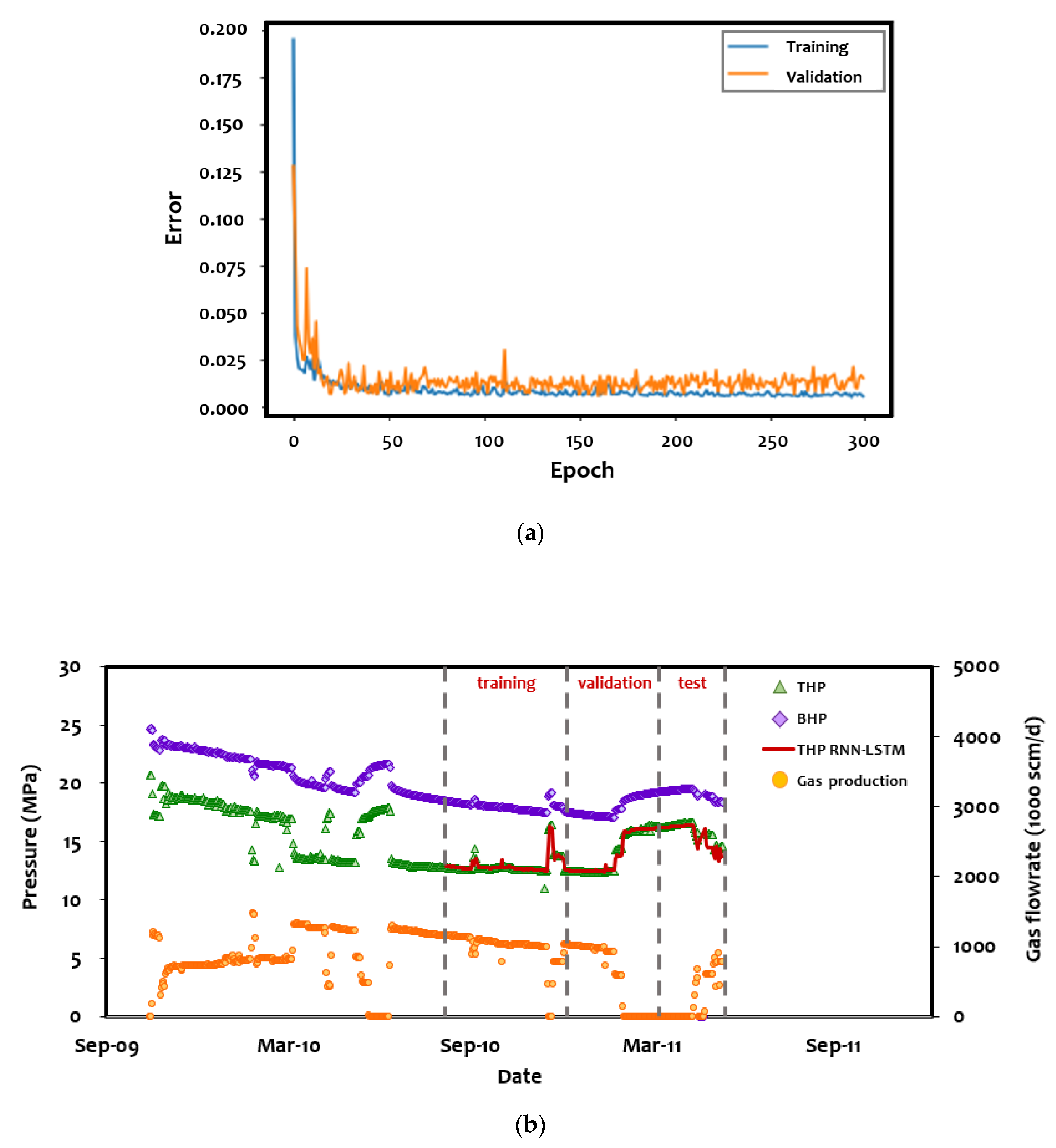
The number of production data points in Period A is 575, which is used to generate 275 datasets with an input sequence length (τ) of 300. The datasets were split such that 125 were used for training, 100 were used for validation, and 50 were used as the test dataset. Figure 7 shows the results of the RNN-LSTM training: Figure 7a shows the loss function versus the epoch, and Figure 7b shows a comparison of the trained results and field pressure data. It can be confirmed that the training was successfully accomplished without overfitting, and the trained RNN model can effectively predict the measured THP behavior in Period A. The MAE values of the training, validation, and test data were estimated as 0.00787, 0.0059, and 0.01586, respectively.

Figure 7. Training results of the RNN-LSTM for Process 1: (a) Loss function versus epoch, and (b) comparison of the tubing head pressure (THP) model results and field data (modified from Ki et al. [25]).

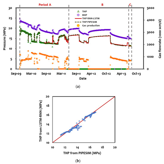
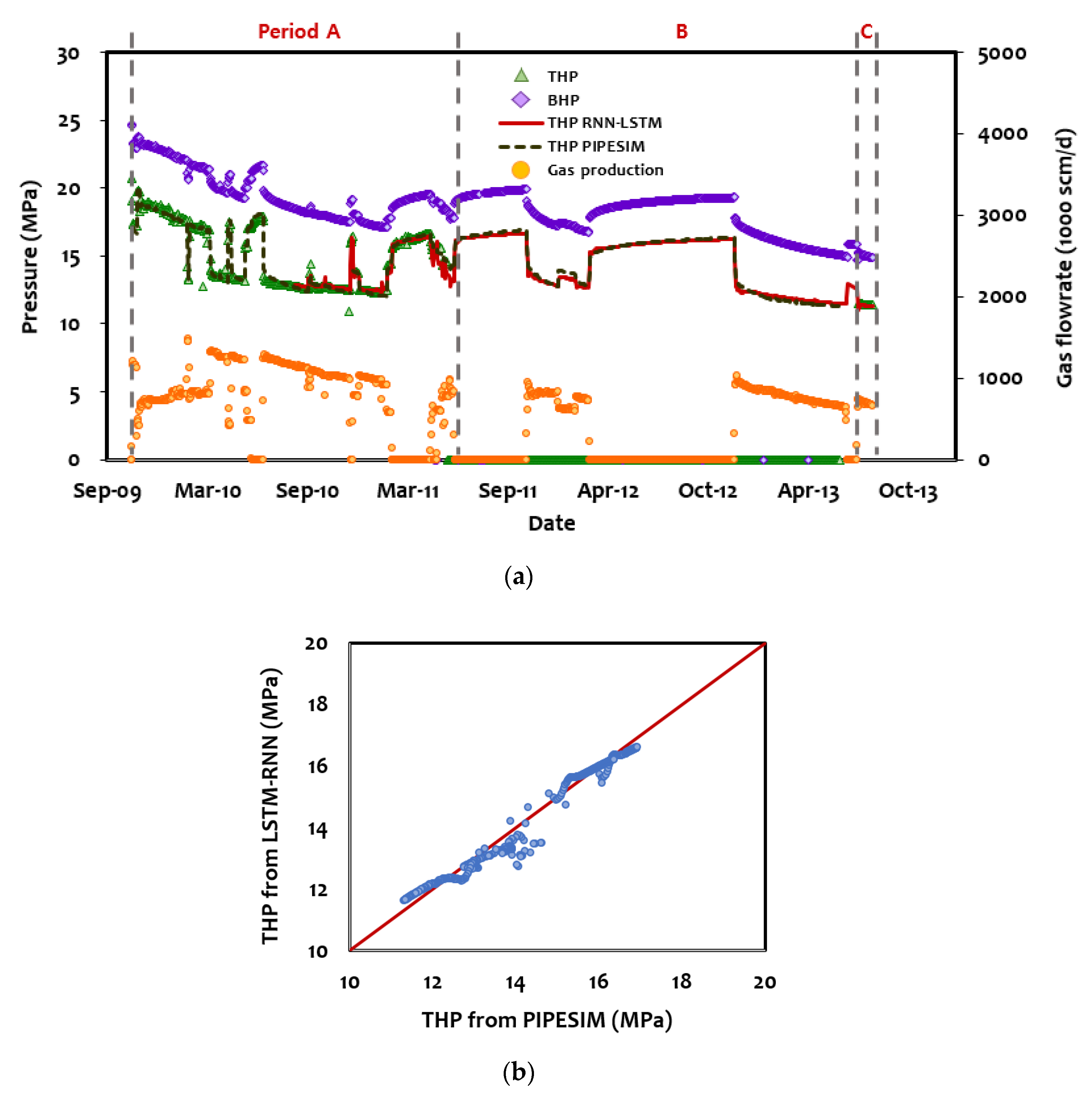
The trained RNN model was used to predict the THP in Periods B and C, as shown in Figure 8. These predictions were also compared with the estimation obtained using PIPESIM software. The differences in the THP during Period B obtained with the RNN model and PIPESIM software are compared in Figure 8b; the MAPE is only 1.53% with a standard deviation of 1.37%. In addition, the difference between the predicted and measured THP in Period C is negligible, thereby verifying that the developed RNN-LSTM model is a highly reliable predictive model. Therefore, it can be concluded that the missing THP data were successfully restored.

Figure 8. Comparison of THP predictions in Period B: (a) THP prediction profile, and (b) comparison between the results of the RNN-LSTM and PIPESIM models (modified from Ki et al. [25]).

3.4. Process 2: THP Prediction during Period F

Period F in Figure 2 is the only long-term buildup interval in more than four years of production operation after Period C, except for the very short shut-ins in Periods D and E. The THP measurements were not performed properly owing to the malfunctioning of the gauge during the entirety of Period F; however, the THP values were measured correctly in the subsequent Period G. In Process 2, an RNN-LSTM model was constructed to predict the THP values in Period F by employing the THP data restored in Process 1; the THPs in Periods A to E were used as the training, validation, and test datasets for Process 2.

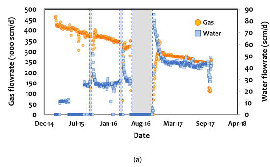
It should be carefully considered that the formation water production commenced during Period E. Water production affects the pressure drop through the well system, and thus the effect of water production should be reflected in some of the input features of the RNN-LSTM model. One simple method to accomplish this is to introduce the equivalent gas rate concept, which describes the pressure drop due to the water production in addition to the gas flow rate. In other words, the equivalent gas flow rate has the same pressure drop as that caused by the multiphase flow of gas and water in the tubing. Figure 9 shows the preprocess for establishing the equivalent gas rate. Figure 9a shows the water and gas production profiles after water breakthrough; there are three buildup periods, as indicated by the shaded areas. It is also notable that there are some missing values in the water production record around the 15 July, which is attributed to missed recordings in the operation field.

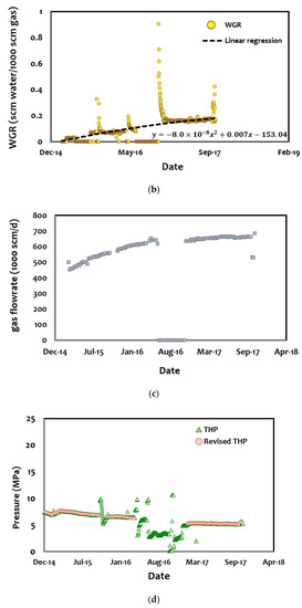
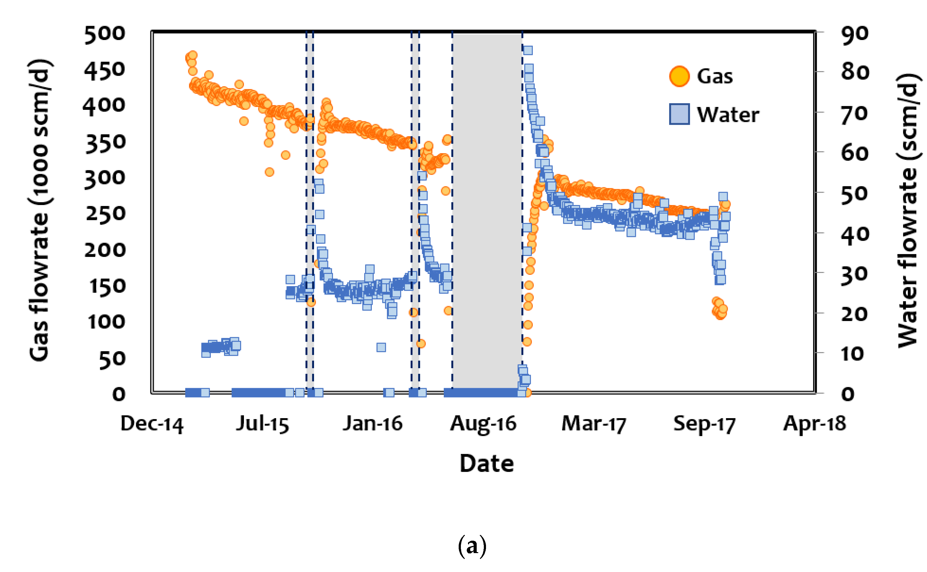
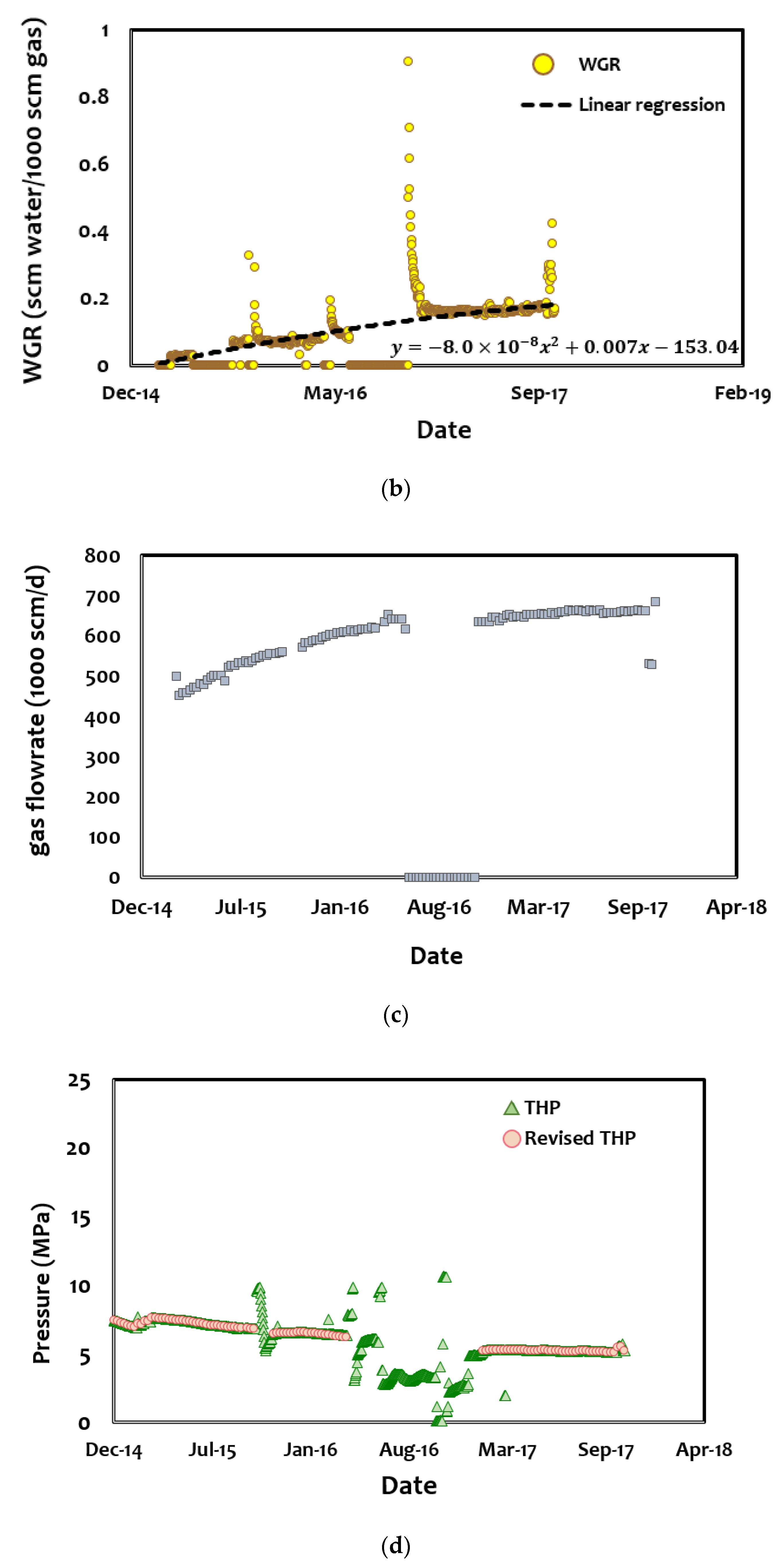
Figure 9. Data preprocessing during the water production period: (a) Water and gas rate profiles, (b) water–gas ratio profile, (c) equivalent gas rate, and (d) THP preprocessing.

When the well was reopened after each buildup, water production started with a peak rate followed by a rapid decline, while the gas rate exhibited the opposite behavior. As explained in the previous section, this phenomenon is attributed to water invasion into the reservoir from the wellbore after a shut-in. The water–gas ratio (WGR) was used to model the water production trend, as shown in Figure 9b, in which a second-order polynomial fitting was adopted. If the trend of rapid decline in the water production after buildup is ignored, the fitting is sufficient to model the overall water production trend during the flowing periods.

To calculate the equivalent gas flow rate, a sensitivity analysis of the pressure drop was conducted using PIPESIM with controllable parameters: gas flow rates of 100, 200, 400, 550, and 700$\times$10³ scm/d; WGRs of 0, 0.05, 0.1, 0.15, and 0.22 scm water/1000 scm gas; THPs of 4.5, 6.0, and 7.5 MPa, which cover the actual range of the observed production. A proxy model based on the sensitivity data was generated to estimate the gas flow rate based on various pressure drop, WGR, and THP values. Then, the model was used to determine the equivalent gas flow rate under the condition of WGR = 0, which reproduces the observed pressure drop. Figure 9c shows the resulting equivalent gas flow rate.

Figure 9d shows the original THP profile and its preprocessed profile during the water production period. Outliers in the gas rate and THP data, such as high fluctuations during shut-ins and re-openings of the well, were excluded from the entire dataset for simplicity and consistency with the dataset before the water breakthrough. The two early shut-ins in Figure 9a were removed from the preprocessed data because the intervals were too short to be considered, and those intervals were replaced with interpolated data using the flow data in the vicinity of the shut-ins.

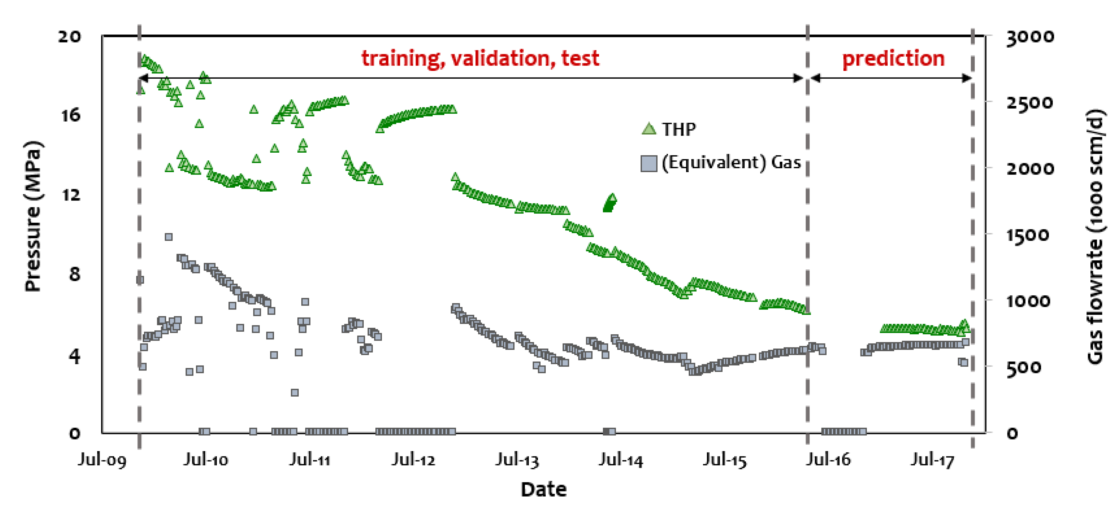
Figure 10 shows the datasets used for the model training and prediction in Process 2. The dataset for the model training includes the training, validation, and testing data. After the RNN-LSTM model is trained, the THP prediction is performed for the prediction interval. There are four input features: THP, the difference between the THP values at adjacent time steps, the equivalent gas rate, and the cumulative gas production in Equation (14). The output target is the difference between the THP at the $t$th and ($t+1$)th time steps in Equation (15). It should be noted that the Qg and cumulative gas data at the ($t+1$)th time step were also included in the input data to improve the training efficiency and accuracy.

$$\mathrm{Input}: {\{\mathrm{THP}}_{t-\tau +i},\Delta \mathrm{P}(={\mathrm{THP}}_{t-\tau +i}-{\mathrm{THP}}_{t-\tau +i-1}),{\mathrm{Qg}}_{t-\tau +i+1},{\mathrm{Cumulative}\mathrm{gas}}_{t-\tau +i+1}|1\le i\le \tau \}$$

(14)

$$\mathrm{Output}:\Delta \mathrm{P}(={\mathrm{THP}}_{t+1}-{\mathrm{THP}}_t)$$

(15)

Figure 10. Revised dataset in Process 2.

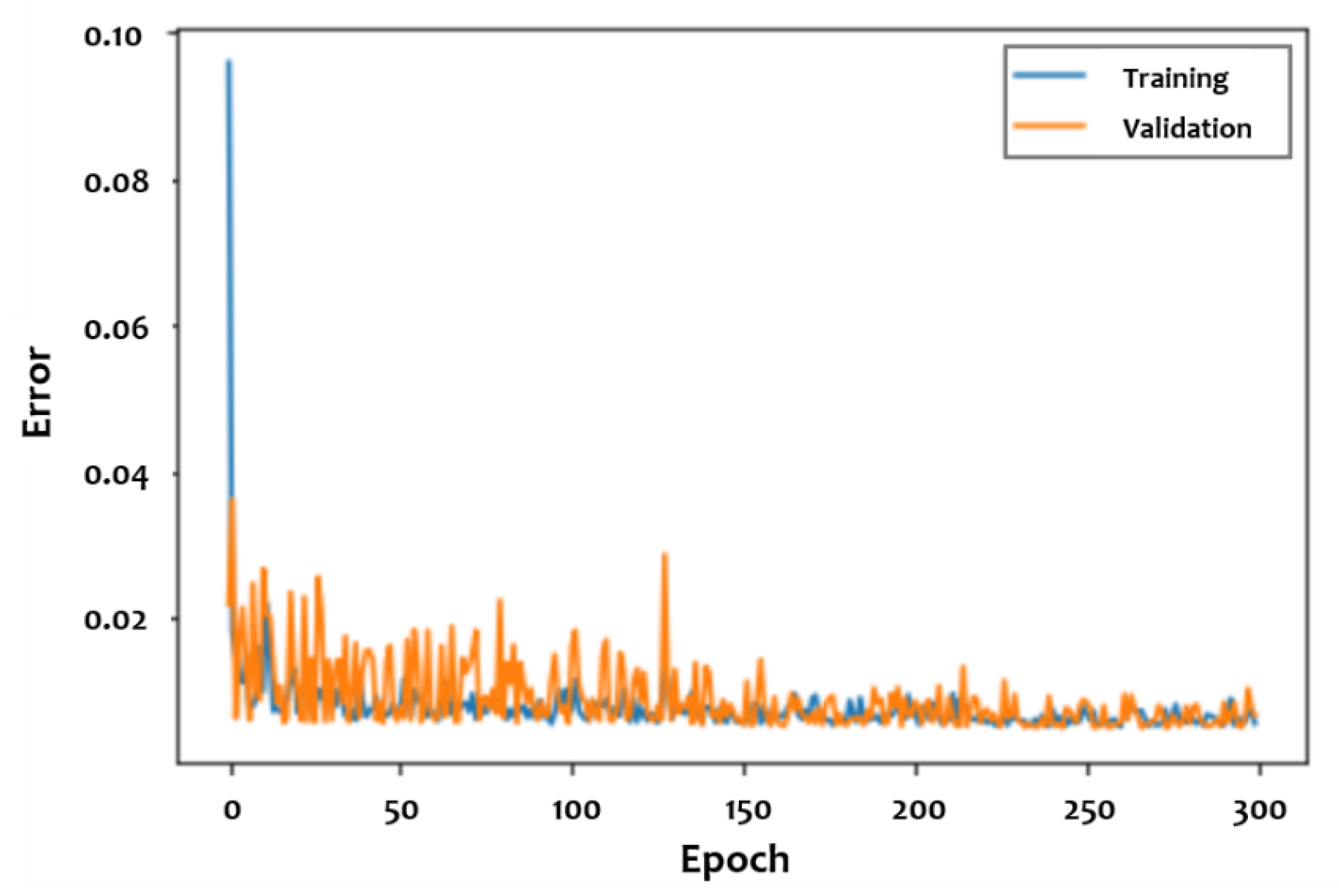
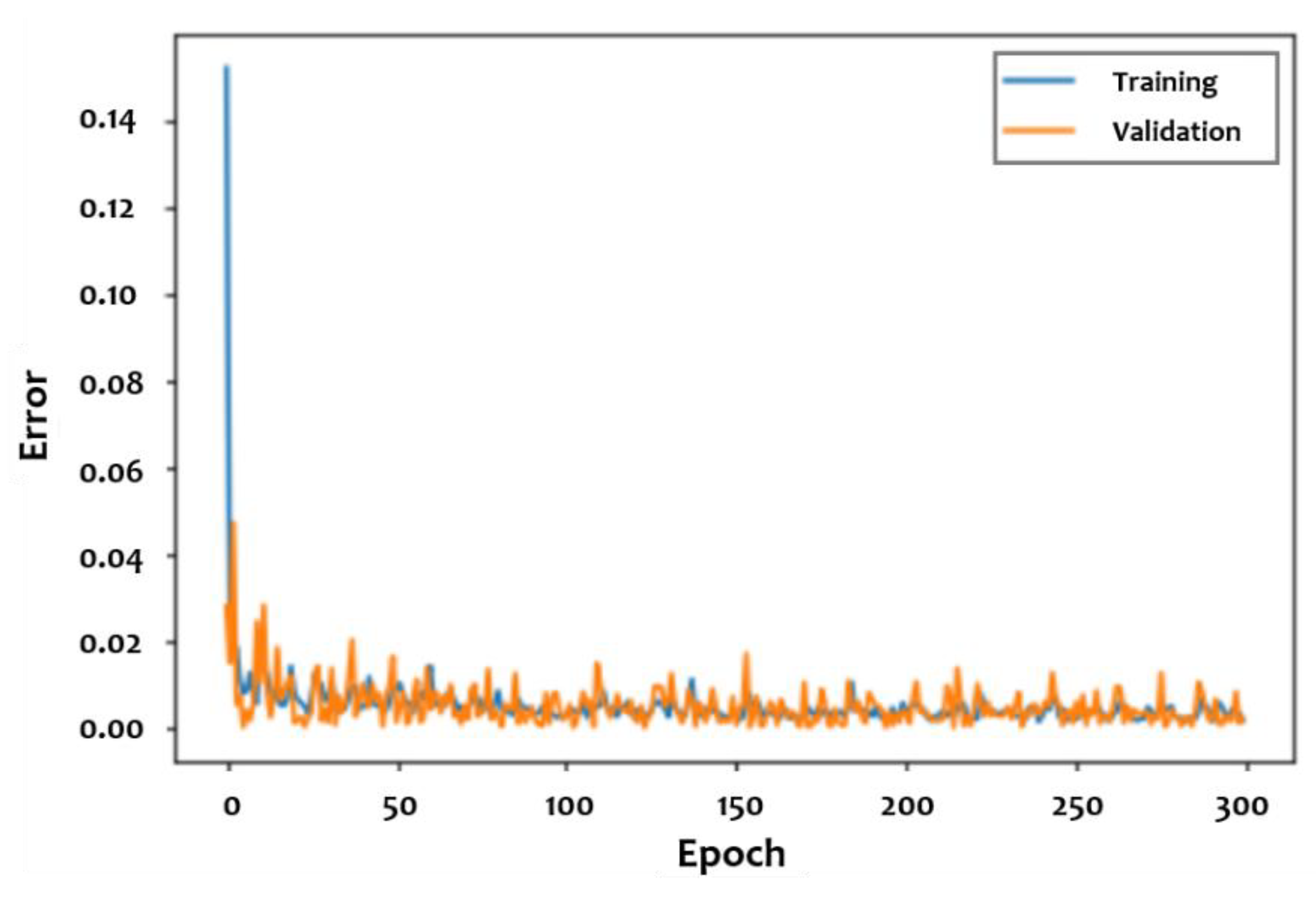
The datasets were resampled with weekly data for training simplicity, and split into training, validation, and test datasets at ratios of 80%, 10%, and 10%, respectively. The datasets were normalized according to Equation (9). The length of the input sequence is 180, which seems sufficiently long to reflect the effect of previous long-term shut-ins on the later pressure and flow rate behaviors. The hyperparameters for the model structure and its training are listed in Table 2. Figure 11 shows the training and validation errors with respect to the epochs. The training results show a fairly good match, as the MAE values are 0.00504, 0.00484, and 0.00799 for the normalized training, validation, and test data, respectively, as summarized in Table 3.

Figure 11. Error functions for the RNN-LSTM training in Process 2.

Table 3. Error functions for Process 2.

Dataset	MAE (Unitless)
Training data	0.00504
Validation data	0.00484
Test data	0.00799

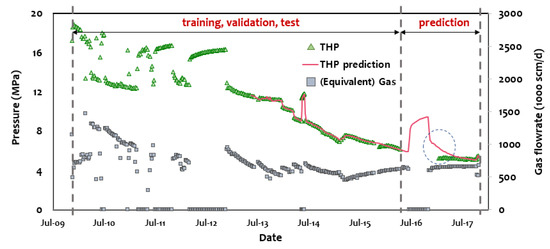
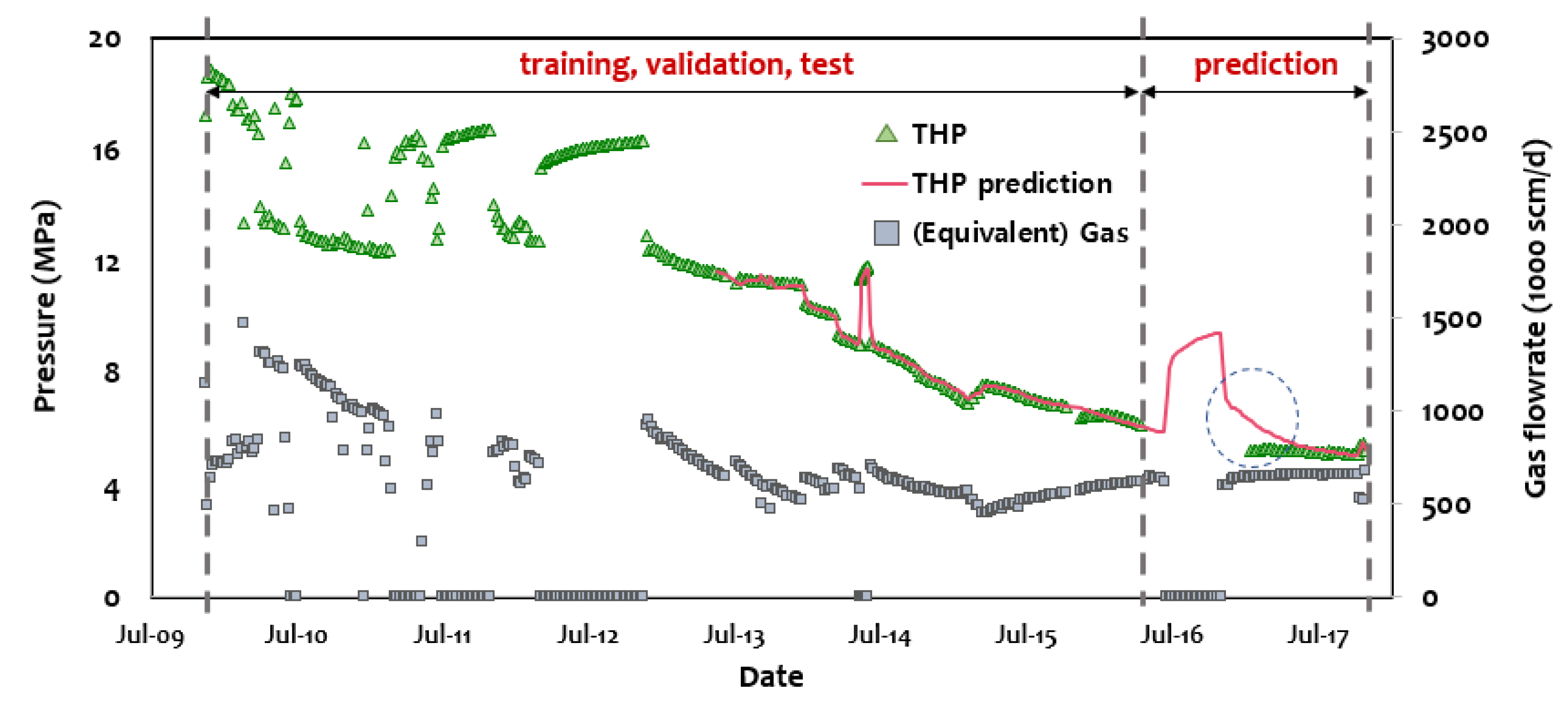
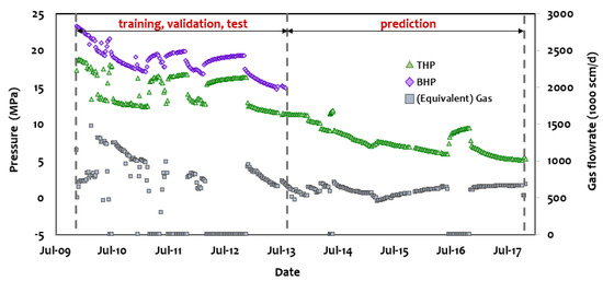
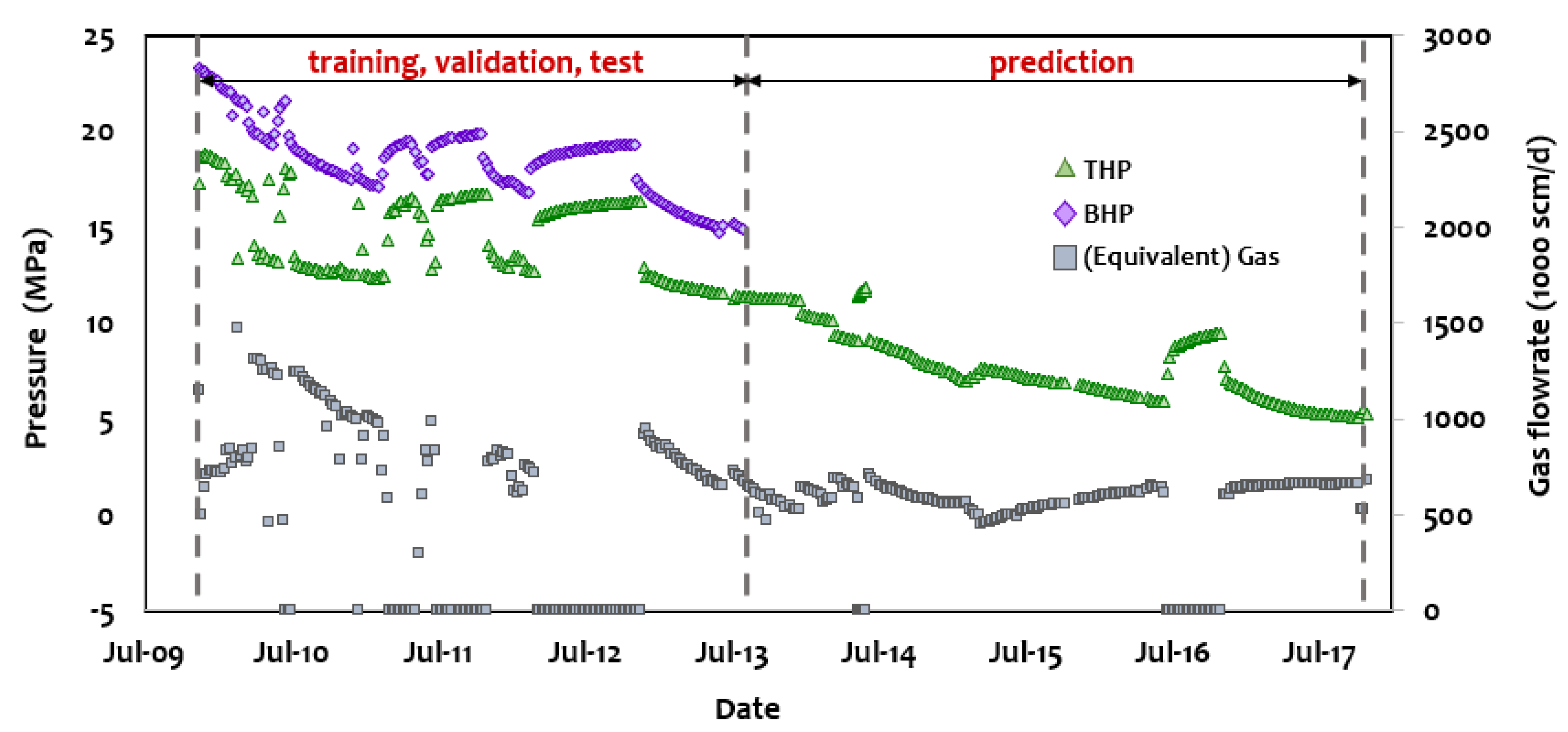
Figure 12 shows a comparison between the predicted THP values and the measured data. It is clear that the RNN-LSTM model has been fairly well trained in terms of the matches in the training, validation, and test datasets. The trained model generated THPs for the prediction interval, which included long shut-in and subsequent production periods. The shapes of the pressure buildups appear very similar to those of the shut-ins in the early part of the training data. There are, however, some large deviations at early flowing times after the long shut-in period (see the dotted circle in Figure 12). This seems to be attributable to the unstable behavior of the multiphase flow after the shut-in. As mentioned above, a shut-in can cause gravity segregation of the multiphase mixture in the wellbore, which can result in productivity loss with water intrusion into the reservoir. Therefore, the measured data in the dotted circle are regarded as less reliable than that in the rest of Period G in Figure 2. The data for the later part of Period G are preferable for use when evaluating the predicted results because this data appears to represent an operation condition in which the productivity has been recovered through long-term and stable production. The similarity between the measured and predicted THPs in the later part of Period G validates the applicability of the procedure in Process 2.

Figure 12. THP prediction results for Process 2.

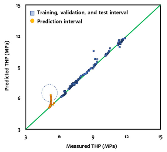
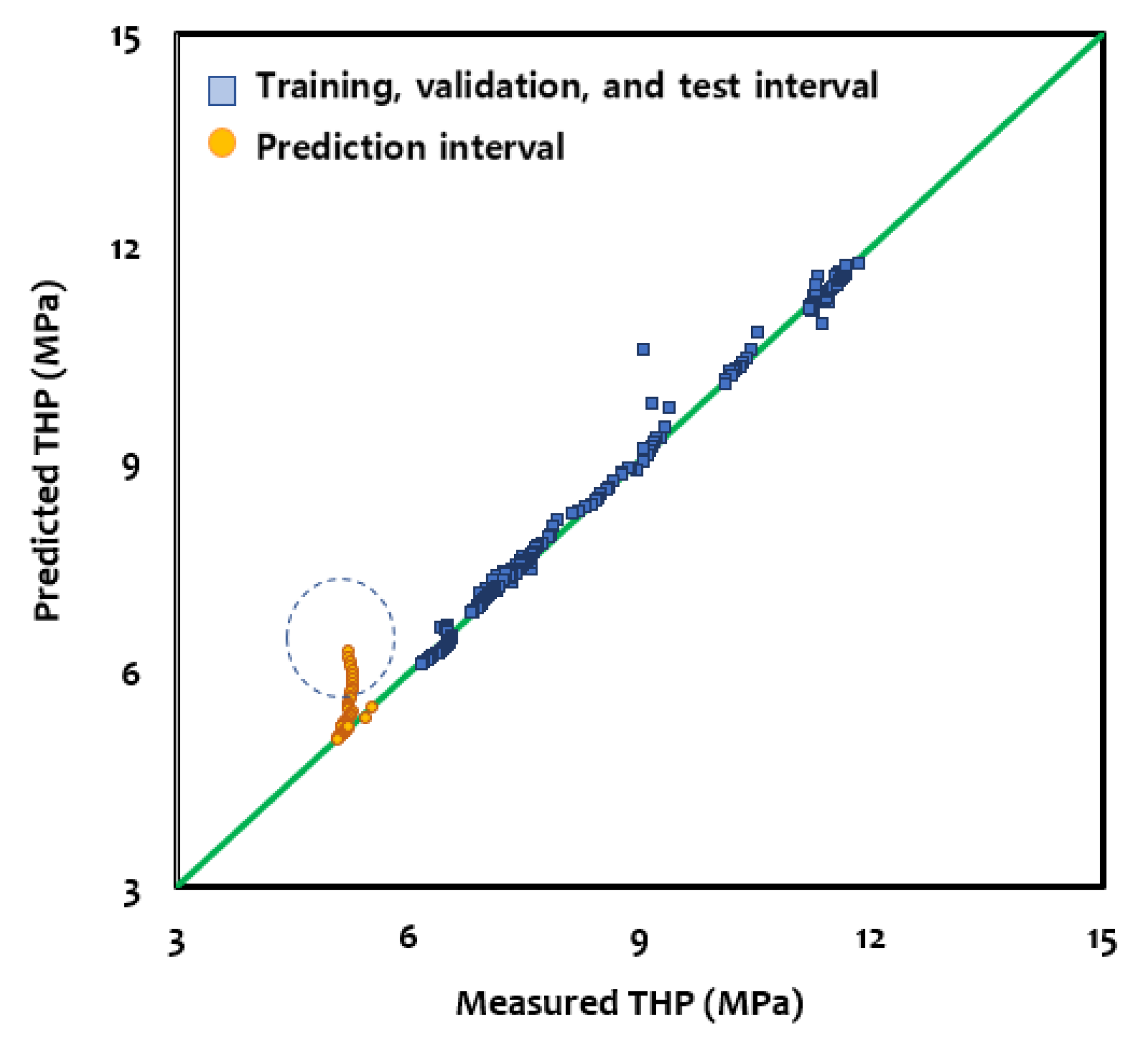
Figure 13 shows a comparison of the predicted and measured THPs. The matches of the training, validation, and test datasets are very good, with an MAE of 0.09 MPa and an MAPE of 1.04%, as summarized in Table 4. This means that the predicted THP is accurate within an error of 1.04%. The MAE for the prediction interval is 0.27 MPa, which corresponds to an MAPE of 5.18%. The dotted circle in Figure 13 corresponds to the dotted circle in Figure 12. When the data in the dotted circle are excluded, the MAE is reduced to 0.05 MPa and the MAPE is 0.96%. In other words, the prediction is very accurate in the later part of the production period (Period G in Figure 2). It is also notable that the concept of the equivalent gas flow rate is shown to be an efficient way to handle multiphase flow data, especially in the case of water production in the middle or later part of the operation period.

Figure 13. Comparison of predicted and measured THP values.

Table 4. Prediction errors in Process 2.

	MAE (MPa)	MAPE (%)
Training, testing, validation interval	0.09	1.04
Prediction interval	0.27	5.18
Prediction interval without the data in the dotted circle	0.05	0.96

3.5. Process 3: BHP Prediction during Periods D to G

In this process, the BHPs in Periods D to G in Figure 2 are predicted based on the results of Processes 1 and 2. Reliable BHP predictions are helpful to inform the decision-making process for future operations utilizing traditional analysis techniques such as reservoir simulations, material balance calculations, and rate transient analyses. In particular, Period F is the last shut-in data in the given dataset, and thus the shut-in information is directly related to the average reservoir pressure, which is essential for forecasting the future performance of the reservoir.

The input data are composed of four features: the THP, the difference between the THP and BHP at the same time step, the equivalent gas rate, and the cumulative gas production in Equation (16); the output target is the difference between the THP and BHP at the ($t+1$)th time step given in Equation (17). It should be noted that the THP, Qg, and cumulative gas data at the ($t+1$)th time step are also included in the input data to improve the training efficiency.

$$\mathrm{Input}:{\{\mathrm{THP}}_{t-\tau +i+1},\Delta \mathrm{P}(={\mathrm{BHP}}_{t-\tau +i}-{\mathrm{THP}}_{t-\tau +i}),{\mathrm{Qg}}_{t-\tau +i+1},{\mathrm{Cumulative}\mathrm{gas}}_{t-\tau +i+1}|1\le i\le \tau \}$$

(16)

$$\mathrm{Output}:\Delta \mathrm{P}(={\mathrm{BHP}}_{t+1}-{\mathrm{THP}}_{t+1})$$

(17)

To ensure the RNN-LSTM model runs efficiently, the data were resampled with an interval of 7 days while preserving the characteristics of the production profile. Figure 14 shows the revised data. The datasets are split into two parts: one for training the RNN-LSTM model and the other for predicting the missing BHP data, as shown in Figure 14. The dataset for the model training includes training, validation, and testing data. After the RNN-LSTM model was trained, the BHP prediction was performed for the prediction interval.

Figure 14. Revised dataset in Process 3.

The datasets were split into training, validation, and test datasets with ratios of 80%, 10%, and 10%, respectively; the length of one input sequence is 100. The hyperparameters for the RNN-LSTM training are listed in Table 2. Figure 15 shows the training and validation errors with respect to the epoch. The MAEs of the final model are 0.00206, 0.00011, and 0.00052 for the normalized training, validation, and test data, respectively (Table 5). The fact that the validation error is much smaller than the training error indicates that the optimized model ensures the minimum validation error among the trained models. The error trends in Figure 15 indicate that the RNN-LSTM model was trained with high stability, although there are many scattered points in the training data as shown in Figure 14.

Figure 15. Error functions of the RNN-LSTM for Process 3.

Table 5. Error functions for Process 3.

Dataset	MAE
Training data	0.00206
Validation data	0.00011
Test data	0.00052

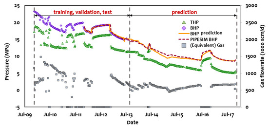
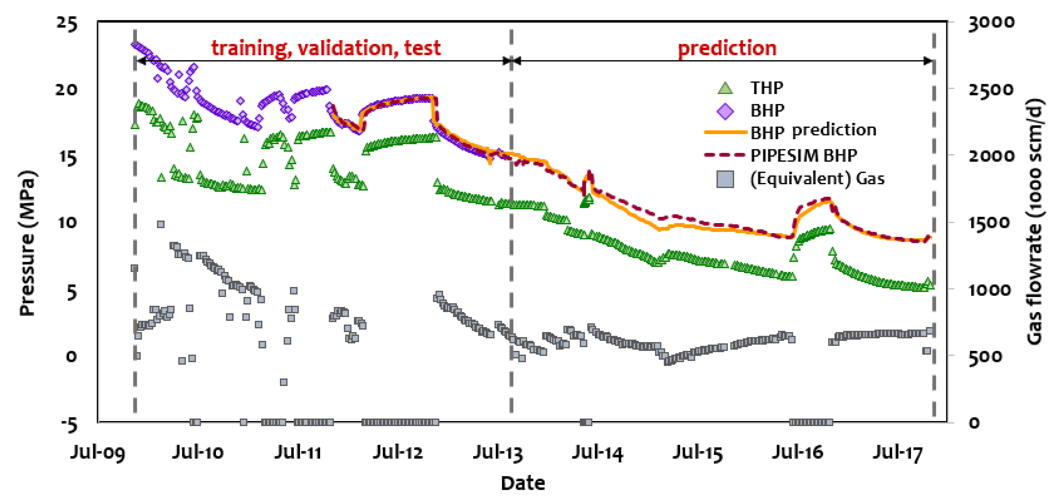
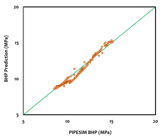
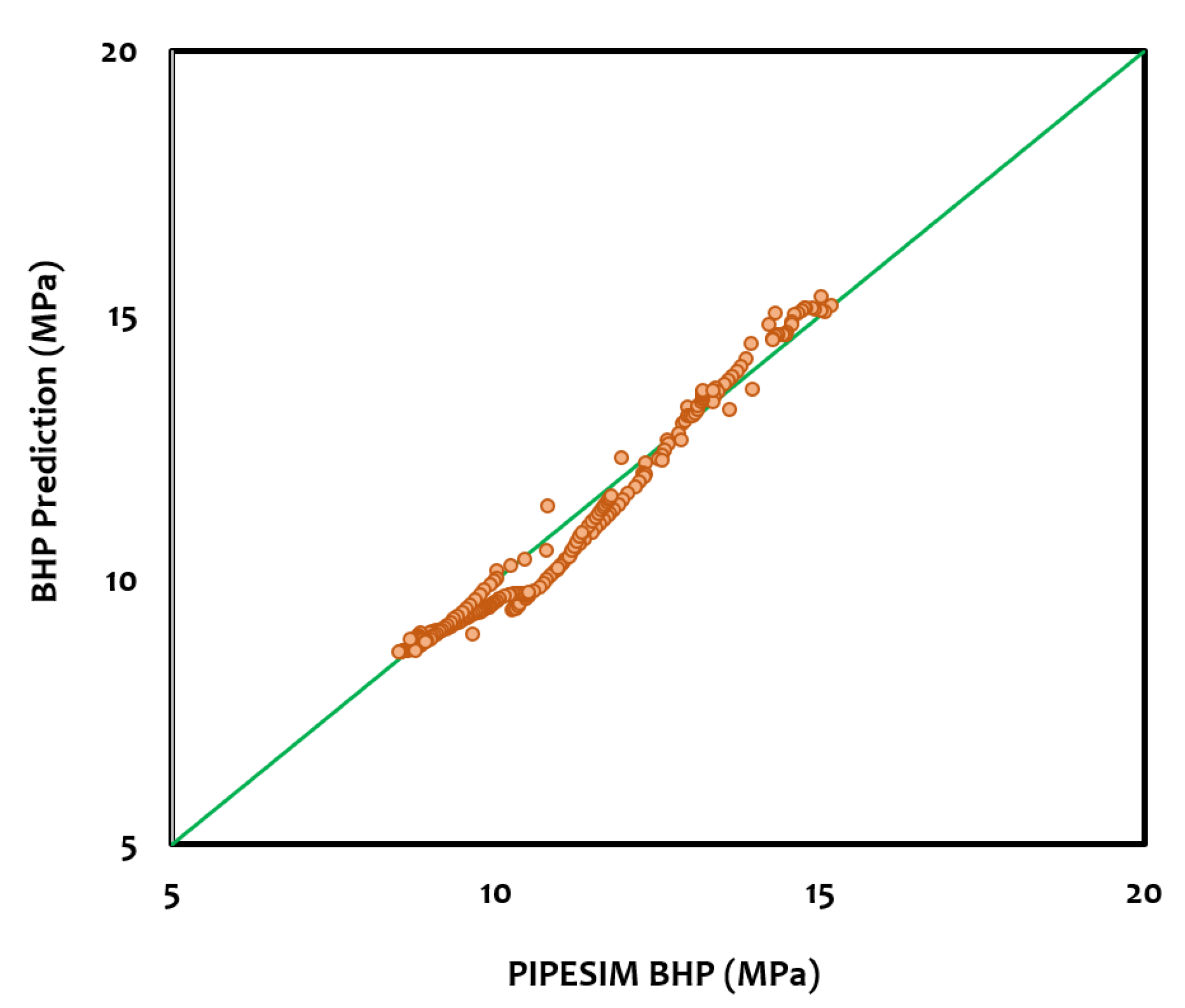
Figure 16 shows the predicted BHPs compared with the results calculated using PIPESIM. The comparison shows similarity in the trends of the results between the RNN-LSTM model and PIPESIM, although there are larger deviations between July 2014 and July 2015 and small deviations in the buildup period around July 2016. The difference between the BHPs obtained with the RNN-LSTM model and those obtained with PIPESIM in the prediction interval are compared in Figure 17, and Table 6 summarizes the corresponding absolute and relative errors. The MAE is 0.31 MPa with a maximum error of 0.84 MPa, which corresponds to an MAPE of 2.77% and a maximum relative error of 8.11%. Considering that the prediction interval is quite long, the RNN-LSTM model performs well in predicting the missing part of the BHP data.

Figure 16. Bottom-hole pressure (BHP) prediction results for Process 3.

Figure 17. Comparison of the predicted and calculated BHP values.

Table 6. Prediction errors for Process 3.

	Absolute Error (MPa)	Absolute Percentage Error (%)
Mean	0.31	2.77
Standard deviation	0.23	2.17
Max	0.84	8.11

4. Conclusions

THP and BHP data are among the essential information collected from oil and gas fields to optimize the production operation. However, pressure data may frequently be missing in some part of the measurement interval as a result of gauge malfunctions or failures in data management. In this study, three processes were performed using RNN-LSTM models to restore the missing parts of a gas production data series collected over more than eight years. The effect of water production in the latter half of the production period was circumvented by introducing the concept of the equivalent gas rate. The entire dataset was successfully constructed with restoration of the missing data based on the analysis of operational characteristics and the application of artificial intelligence techniques. The prediction results were acceptable with MAPE values of 1.53%, 5.18%, and 2.77% for Processes 1, 2, and 3, respectively. When the disturbance in the pressure response owing to the liquid loading was excluded, the MAPE for Process 2 reduced to 0.96%. Thus, the methodology developed in this study can be applied as a data-driven approach to predict missing pressure data with a reasonable error.

References

- Hansen, L.; Pedersen, S.; Durdevic, P. Multi-phase flow metering in offshore oil and gas transportation pipelines: Trends and perspectives. Sensors 2019, 19, 2184. [Google Scholar] [CrossRef] [Scilit] [PubMed]
- Kanshio, S. A review of hydrocarbon allocation methods in the upstream oil and gas industry. J. Pet. Sci. Eng. 2020, 184, 1–13. [Google Scholar] [CrossRef] [Scilit]
- Carvajal, G.; Maucec, M.; Cullick, S. Intelligent Digital Oil and Gas Fields; Gulf Professional Publishing: Oxford, UK, 2018; pp. 75–100. [Google Scholar]
- Gelman, A.; Hill, J. Data Analysis using Regression and Multilevel/Hierarchical Models; Cambridge University Press: Cambridge, UK, 2006; pp. 529–544. [Google Scholar]
- Shalev-Shwartz, S.; Ben-David, S. Understanding Machine Learning from Theory to Algorithms; Cambridge University Press: Cambridge, UK, 2014; pp. 19–24. [Google Scholar]
- Kotezhekov, V.; Margarit, A.; Pustovskih, A.; Sitnikov, A. Development of automatic system for decline analysis. In Proceedings of the SPE Russian Petroleum Technology Conference, Moscow, Russia, 16–18 October 2017. SPE 187755. [Google Scholar]
- Vyas, A.; Datta-Gupta, A.; Mishra, S. Modeling Early Time Rate Decline in Unconventional Reservoirs Using Machine Learning Techniques. In Proceedings of the Abu Dhabi International Petroleum Exhibition & Conference, Abu Dhabi, UAE, 13–16 November 2017. SPE 188231. [Google Scholar]
- Bowie, B. Machine Learning Applied to Optimize Duvernay Well Performance. In Proceedings of the SPE Canada Unconventional Resources Conference, Calgary, Alberta, 13–14 March 2018. SPE 189823. [Google Scholar]
- Jacobs, T. Automated drilling technologies showing promise. J. Pet. Technol. 2015, 67, 50–55. [Google Scholar] [CrossRef] [Scilit]
- Unrau, S.; Torrione, P.; Hibbard, M.; Smith, R.; Olesen, L.; Watson, J. Machine Learning Algorithms Applied to Detection of Well Control Events. In Proceedings of the SPE Kingdom of Saudi Arabia Annual Technical Symposium and Exhibition, Dammam, Saudi Arabia, 24–27 April 2017. SPE 188104. [Google Scholar]
- Guyaguler, B.; Horne, R.; Rogers, L. Optimization of well placement in a Gulf of Mexico waterflooding project. SPE Reserv. Eval. Eng. 2002, 5, 229–236. [Google Scholar] [CrossRef] [Scilit]
- Min, B.; Park, C.; Kang, J.; Park, H.; Jang, I. Optimal well placement based on artificial neural network incorporating the productivity potential. Energy Sources Part A 2011, 33, 1726–1738. [Google Scholar] [CrossRef] [Scilit]
- Sayyafzadeh, M. Reducing the computation time of well placement optimisation problems using self-adaptive metamodeling. J. Pet. Sci. Eng. 2017, 151, 143–158. [Google Scholar] [CrossRef] [Scilit]
- Jang, I.; Oh, S.; Kim, Y.; Park, C.; Kang, H. Well-placement optimisation using sequential artificial neural networks. Energy Explor. Exploit. 2018, 36, 433–449. [Google Scholar] [CrossRef] [Scilit]
- Ahn, S.; Park, C.; Kim, J.; Kang, J. Data-driven inverse modeling with a pre-trained neural network at heterogeneous channel reservoirs. J. Pet. Sci. Eng. 2018, 170, 785–796. [Google Scholar] [CrossRef] [Scilit]
- Lee, K.; Lim, J.; Ahn, S.; Kim, J. Feature extraction using a deep learning algorithm for uncertainty quantification of channelized reservoirs. J. Pet. Sci. Eng. 2018, 171, 1007–1022. [Google Scholar] [CrossRef] [Scilit]
- Osman, E.; Ayoub, M.; Aggour, M. An Artificial Neural Network Model for Predicting Bottomhole Flowing Pressure in Vertical Multiphase Flow. Proceeding of the SPE Middle East Oil and Gas Show and Conference, Manama, Bahrain, 12–15 March 2005. SPE 93632. [Google Scholar]
- Jahanandish, I.; Salimifard, B.; Jalalifar, H. Predicting bottomhole pressure in vertical multiphase flowing wells using artificial neural networks. J. Pet. Sci. Eng. 2011, 75, 336–342. [Google Scholar] [CrossRef] [Scilit]
- Ehrahimi, A.; Khamehchi, E. A robust model for computing pressure drop in vertical multiphase flow. J. Nat. Gas Sci. Eng. 2015, 26, 1306–1316. [Google Scholar] [CrossRef] [Scilit]
- Spesivtsev, P.; Kharlashkin, A.; Sinkov, K. Study of the transient terrain-induced and severe slugging problems by use of the drift-flux model. SPE J. 2017, 22, 1570–1584. [Google Scholar] [CrossRef] [Scilit]
- Yu, Y.; Si, X.; Hu, C.; Zhang, J. A review of recurrent neural networks: LSTM cells and network architectures. Neural Comput. 2019, 31, 1235–1270. [Google Scholar] [CrossRef] [Scilit] [PubMed]
- Hochreiter, S.; Schmidhuber, J. Long short-term memory. Neural Comput. 1997, 9, 1725–1780. [Google Scholar] [CrossRef] [Scilit] [PubMed]
- Sagheer, A.; Kotb, M. Time series forecasting of petroleum production using deep LSTM recurrent networks. Neurocomputing. 2019, 323, 203–213. [Google Scholar] [CrossRef] [Scilit]
- Tian, C.; Horne, R. Applying machine learning techniques to interpret flow rate, pressure and temperature data from permanent downhole gauges. SPE Reserv. Eval. Eng. 2019, 22, 386–401. [Google Scholar] [CrossRef] [Scilit]
- Ki, S.; Seo, J.; Kwon, O.; Jang, I. Prediction of missing tubing head pressure using recurrent neural network. J. Korean Soc. Min. Energ. Resour. Eng. 2019, 56, 416–426. [Google Scholar] [CrossRef] [Scilit]
- KNOC. Reserves Estimation Report; Korea National Oil Corporation: JUNG-GU, Korea, unpublished.
- RNN, LSTM & GRU. Available online: http://dprogrammer.org/rnn-lstm-gru (accessed on 13 July 2020).
- Schlumberger. PIPESIM Fundamentals Training and Exercise Guide; Schlumberger: Houston, TX, USA, 2017. [Google Scholar]
- Beggs, H. Production Optimization Using Nodal Analysis; OGCI Publications: Tulsa, OK, USA, 1991; p. 88. [Google Scholar]
- Tensorflow. Available online: https://www.tensorflow.org (accessed on 13 July 2020).
© 2020 by the authors. Licensee MDPI, Basel, Switzerland. This article is an open access article distributed under the terms and conditions of the Creative Commons Attribution (CC BY) license (http://creativecommons.org/licenses/by/4.0/).