Dependence of Extreme Values, VaR, and Contagion During the COVID-19 Period: Analysis Using the Copula-GARCH Approach

Abstract

The present study investigates extreme co-movements and financial contagion across a broad set of global financial markets, including ten developed and emerging stock market indices, commodities (gold and oil), and cryptocurrencies (Bitcoin), over the period from January 2007 to May 2023. In the context of the increasing interconnectedness of global financial markets, it is imperative to comprehend the propagation of systemic shocks across asset classes for the purpose of effective risk management. In order to achieve this objective, a Copula-GARCH framework is employed, in which the Student’s t-copula is selected for its superior ability to capture nonlinear dependence and tail co-movements. The analysis compares dependence structures during the pre-crisis and the COVID-19 crisis periods. The present study diverges from the majority of previous research in its utilisation of a combined approach, integrating Copula-GARCH modelling with wavelet analysis. This novel method is employed to collectively examine tail dependence and multi-scale contagion dynamics, thereby facilitating a more comprehensive evaluation of financial interconnectedness during periods of market stress. The empirical evidence indicates significant and largely symmetric tail dependence across the majority of market pairs. This finding suggests the presence of stronger co-movements during periods of extreme market conditions, a phenomenon that was particularly evident throughout the course of the global pandemic. The robustness of these findings is further confirmed by wavelet analysis, which provides a multi-scale perspective on shock transmission across markets. The results demonstrate that financial contagion intensified during the pandemic, with important implications for international portfolio diversification and risk management. Furthermore, the role of gold as a potential safe-haven asset during periods of severe financial stress is highlighted, providing valuable insights for investors and policymakers.

1. Introduction

The progressive integration of global financial markets, driven by the removal of regulatory barriers and technological advancements, has fundamentally altered the landscape of international investment. As is evident from the extant literature (see Zivot & Andrews, 1992), the interconnectedness of financial markets offers significant opportunities for portfolio optimisation and risk diversification. However, it simultaneously introduces complex challenges in modelling the joint distribution of risk factors. It is an established fact that traditional financial risk management has long been dominated by multivariate statistical models assuming a joint normal distribution. This reliance on the correlation coefficient as a primary measure of dependence is predicated on the assumption that associations between random variables can be fully described by normal marginal distributions (Nelsen, 2006).

However, empirical evidence from financial time series has consistently revealed the presence of “heavy tails,” asymmetry, and kurtosis, which challenge the validity of the normality assumption. It has been demonstrated by seminal studies by researchers such as Dacorogna and Pictet (1997), as well as Danielsson and de Vries (2000), that the normal distribution is inadequate for capturing “tail dependence”, the tendency of markets to crash simultaneously during extreme events. This limitation assumes particular significance during systemic shocks, where the underestimation of joint extreme risks can result in catastrophic portfolio losses (Zayati et al., 2016). Consequently, a controversial yet essential debate has emerged in the research field regarding the most effective multivariate distributions for capturing the complex co-movements that signify financial contagion.

In order to address these methodological shortcomings, the present study invokes Sklar’s theorem (Sklar, 1959) in order to employ copula functions. The primary advantage of the copula approach is its flexibility, which allows for the separate modelling of marginal distributions and the underlying dependence structure. In contrast to linear correlation, copulas are resistant to data transformations and can capture not only the degree but also the specific structure of tail dependence (Cherubini et al., 2004). Patton’s (2006) seminal work constituted a significant extension of copula theory by introducing dynamic conditional copulas, thereby enabling parameters to vary over time. This evolution has proven instrumental in analysing how market dependencies fluctuate during periods of high volatility (Fantazzini, 2008; Rodriguez, 2007). Recent literature has further validated the Copula-GARCH framework as a superior tool for studying nonlinear and asymmetric correlations across diverse financial markets (Yao & Li, 2023; Kumar et al., 2021).

The primary objective of this research endeavour is to undertake a comprehensive investigation into the intensity of financial contagion and extreme co-movements across pre- and post-pandemic periods, encompassing the timeframes preceding and following the advent of the Coronavirus pandemic. The present paper makes two contributions to the extant literature. Firstly, it provides a comprehensive analysis using a uniquely broad sample that includes ten developed and emerging market indexes (China, USA, Japan, France, UK, Germany, Russia, Ukraine, Indonesia, and Brazil), alongside commodities (gold and oil) and cryptocurrencies (Bitcoin), covering the period from 2007 to 2023. Secondly, the robustness of the findings is enhanced by the integration of a sophisticated wavelet methodology, which provides a multi-scale perspective on shock propagation. The principal conclusions of the present study highlight a significant increase in tail dependence during the pandemic and underscore the evolving role of non-traditional assets in global risk management.

The remainder of this paper is organized as follows. Section 2 introduces the theoretical framework of copulas. Section 3 details the data and the empirical Copula-GARCH methodology. Section 4 presents the econometric results and discussion. Section 5 provides a robustness analysis using the wavelet method, and Section 6 concludes the study.

2. Literature Review

2.1. Theoretical Foundations and Channels of Financial Contagion

The definition of financial contagion remains a subject of considerable academic debate. As Eichengreen et al. (1996) have observed, the phenomenon of contagion can be conceptualised as a situation in which the occurrence of a crisis in one country significantly increases the probability of a crisis occurring in another. This concept is further refined by Forbes and Rigobon (2002), who distinguish between “interdependence”—representing stable, long-term linkages—and “contagion,” which involves a significant shift in cross-market correlations following a shock.

Theoretically, these transmissions occur through several well-documented channels. Masson (1998) proposes a classification system which distinguishes between three categories of economic impact: “monsoonal effects” (common external shocks), “spillovers” resulting from fundamental linkages, and “pure contagion” driven by investor behaviour. This phenomenon has been linked to the “wake-up call” effect (Goldstein, 1998) or liquidity shocks, which force institutional investors to liquidate positions across multiple markets simultaneously (Calvo & Reinhart, 1996; Corsetti et al., 1999). Recent studies on the era of the pandemic, including Umar et al. (2022), suggest that these channels have become even more interconnected due to the digitalisation of financial markets, thereby accelerating the speed of shock propagation.

2.2. Financial Contagion and Extreme Market Shocks

The phenomenon of financial contagion has been extensively documented, particularly during periods of systemic crises. It is evident from the seminal studies undertaken by King and Wadhwani (1990) and Calvo and Reinhart (1996) that correlations between markets tend to increase significantly during periods of market downturns in comparison with stable periods. The ongoing global pandemic of the novel virus known as SARS-CoV-2 has offered a unique opportunity to observe these dynamics. Research by Akhtaruzzaman et al. (2021) and Just and Echaust (2020) demonstrated that the health crisis triggered an unprecedented level of international spillover, where shocks in developed markets rapidly propagated to emerging economies, often through nonlinear channels that traditional correlation measures fail to capture. A fundamental difference between the impact of the current pandemic and the Global Financial Crisis of 2008 is the former’s exogenous and non-financial nature. The global health crisis was characterised by a lack of conventional financial triggers, resulting in a simultaneous systemic shock that placed unprecedented stress on safe-haven assets. The distinctive nature of the crisis indicates that contagion was predominantly driven by psychological uncertainty and global lockdowns rather than initial financial imbalances. This necessitates the development of models capable of capturing such rapid and nonlinear shifts in market sentiment.

2.3. The Role of Alternative Assets: Bitcoin, Gold, and Oil

A substantial proportion of recent literature focuses on the safe-haven properties of alternative assets. It is an established fact that gold has historically been regarded as a means of protection against inflation and market downturns (Baur & Lucey, 2010). However, the advent of Bitcoin has resulted in the introduction of a new dimension to the diversification of investment portfolios. In the academic discourse, proponents of Bitcoin have posited that it functions as a form of “digital gold” (Dyhrberg, 2016), thereby offering a safeguard against extreme events. However, studies by Conlon and McGee (2020) in the early stages of the pandemic suggest that Bitcoin’s volatility may limit its hedging effectiveness. In a similar fashion, the relationship between crude oil and stock markets remains intricate. Whilst oil frequently functions as a source of contagion due to its effect on global production costs, its role as a diversifier exhibits significant variation across diverse time scales and market conditions (Broadstock et al., 2014). Moreover, the repercussions of this contagion are especially evident in emerging economies, such as those incorporated in the present study (e.g., Ukraine, Indonesia, and Brazil). It is evident that such markets frequently encounter diminished liquidity and augmented sensitivity to capital flight during periods of global “risk-off” episodes. It is imperative to comprehend the propagation of extreme shocks from developed financial hubs to emerging frontiers, as the fragility of these emerging markets’ financial infrastructures can result in more violent and persistent contagion effects than those observed in more mature markets.

Recent studies have further advanced the analysis of financial contagion by adopting dynamic and multi-scale dependence frameworks. For instance, Zhao and Park (2024) employed a dynamic Copula-EVT-CoVaR approach to investigate bidirectional risk spillovers between the Chinese stock market and other Asian markets. In a similar vein, Wang et al. (2024) proposed a VMD-Vine Copula-CoVaR framework to examine multi-scale dependence and contagion across international financial markets. Recent evidence also highlights the growing importance of contagion channels involving alternative assets. Ibrahim et al. (2024) documented significant volatility contagion among cryptocurrencies, gold, and stock markets before and during the pandemic of Coronavirus Disease 2019 (COVID-19). In addition, recent methodological developments based on flexible copula structures have enhanced the measurement of tail dependence and financial contagion (Saekow et al., 2025). These contributions serve to confirm the increasing relevance of dynamic and nonlinear approaches for the purpose of capturing evolving contagion mechanisms across global financial markets.

2.4. Methodological Advances: Copula-GARCH and Wavelet Analysis

In order to address the limitations of linear correlation, econometric literature has shifted towards the adoption of more flexible frameworks. The Copula-GARCH approach has become the gold standard for modelling asymmetric and tail dependence. Patton (2006) and Jondeau and Rockinger (2006) demonstrated that copulas facilitate the separation of marginal distributions from the dependence structure, rendering them particularly well-suited for the capture of “black swan” events in financial returns. Moreover, the integration of wavelet methodology, as evidenced in the research of Ranta (2013) and Aguiar-Conraria and Soares (2014), enables researchers to decompose financial signals into distinct frequencies. This multi-scale approach is imperative in order to differentiate between short-term fluctuations and long-term fundamental shifts in market integration, thereby furnishing a more granular perspective on the manner in which contagion evolves. Recent applications of these combined methodologies, as evidenced by the work of Alqaralleh and Canepa (2021) and Ben Saïda (2023), have yielded novel insights into the “new normal” of global financial integration. The findings of the study suggest that the pandemic fundamentally altered the risk–return landscape, necessitating more adaptive risk management strategies. The present study contributes to the extant literature by providing a comprehensive analysis of thirteen diverse assets, thereby ensuring that the findings on contagion are robust across both the time and frequency domains.

2.5. Research Gap and Study Contribution

Despite the growing literature on financial contagion and market interconnectedness, several important gaps remain. First, most existing studies focus on a limited set of financial markets or a single asset class, thereby providing only a partial view of international transmission mechanisms. Second, although China has become one of the most influential financial and economic actors worldwide, empirical evidence regarding its dependence structure on a broad range of international financial assets remains relatively limited. Third, previous studies generally rely either on copula-based approaches or wavelet techniques, whereas the combined use of these complementary methodologies remains scarce. Finally, limited attention has been devoted to comparing dependence structures before and during the COVID-19 crisis across multiple asset classes within a unified analytical framework.

To address these gaps, this study investigates the dependence structure between the Chinese stock market and twelve major international financial assets representing stock markets, commodities, exchange rates, and cryptocurrencies. The analysis combines GARCH filtering, copula-based dependence modeling, wavelet coherence analysis, and Value-at-Risk assessment to provide a comprehensive evaluation of financial interconnectedness and contagion dynamics during normal and crisis periods.

3. Materials and Methods

3.1. Data Description

This paper focuses on how the performance of the Chinese market relates to other markets both before and after the COVID-19 crisis, using copula functions and a GARCH-type conditional heteroscedasticity model. Our dataset consists of daily frequency series of stock market indices in US dollars, ranging from 2 January 2007 to 29 May 2023. These indices have been extracted from the MSCIBARRA database provided by Morgan Stanley Capital International BARRA. First, we tested them in their natural logarithm form. Our study included 10 financial markets (USA, Japan, France, Great Britain, Germany, Russia, Ukraine, China, Indonesia, Brazil), as well as the cryptocurrency market (Bitcoin) and two commodity markets (gold and oil).

The selection of the 13 assets in our sample was motivated by their representativeness of global financial interdependence. The ten equity markets (USA, Japan, France, UK, Germany, Russia, Ukraine, China, Indonesia, Brazil) provide a balanced coverage of both developed and emerging economies, thereby allowing us to capture heterogeneous contagion dynamics across different levels of market maturity and liquidity. Gold and oil were included due to their dual role as traditional safe havens and systemic risk transmitters, respectively, which is particularly relevant during global crises. Finally, Bitcoin was selected as the most representative cryptocurrency, given its dominant market capitalization and its increasing role in portfolio diversification debates. This diversified set of assets ensures that our findings are robust and generalizable across equities, commodities, and digital assets, offering a comprehensive framework to analyze contagion channels during systemic shocks.

3.2. Econometric Framework

The estimation proceeds in two stages, following the Canonical Maximum Likelihood (CML) approach proposed by Cherubini et al. (2004). In the first stage, the marginal distributions of each return series are estimated non-parametrically using their Empirical Cumulative Distribution Functions (ECDF), rescaled by n/(n + 1) to ensure the well-definiteness of the log-likelihood function. The standardized residuals obtained from the GARCH(1,1) models are then transformed into uniform variates via this empirical probability integral transform (PIT). In the second stage, the copula parameter θ is estimated by maximizing the copula log-likelihood function given the uniform marginals obtained in the first stage, as described in Equation (14). This two-step semi-parametric approach is implemented in R (version 4.3) using the copula package (Hofert et al., 2020). The CML estimator is consistent, asymptotically normal, and fully efficient under independence (Cherubini et al., 2004). The selection of the optimal copula family is based on the AIC, BIC, and the Cramér–von Mises goodness-of-fit statistic following Genest et al. (2009).

3.2.1. Dependence Modeling: The Copula Approach

Definition: a copula of dimension J is a multivariate distribution function $\mathrm{C}$ that is defined on the hypercube ${[0;1]}^{\mathrm{J}}$ with uniform margins on $[0,1]$.

Theorem: Sklar (1959)’s Theorem:

If F is an n-dimensional distribution function with marginals ${\mathrm{F}}_1,\dots ,{\mathrm{F}}_{\mathrm{J}}$, then there is a J-copula C that satisfies the following equation for every $\mathrm{x}$ in ${\mathrm{R}}_{\mathrm{J}}$

$$\mathrm{F}\left({\mathrm{x}}_1,\dots ,{\mathrm{x}}_{\mathrm{J}}\right)=\mathrm{C}\left({\mathrm{F}}_1\left({\mathrm{x}}_1\right),\dots ,{\mathrm{F}}_{\mathrm{J}}\left({\mathrm{x}}_{\mathrm{J}}\right)\right)$$

(1)

If the marginals ${\mathrm{F}}_1,\dots ,{\mathrm{F}}_{\mathrm{J}}$ are continuous, the copula $\mathrm{C}$ is unique.

The theorem proves the existence of a copula, which serves to describe the multivariate distribution function using its marginals. This copula fully embodies the interdependence of the variables in question. A copula, by definition, is a distribution function with uniform marginal laws, making its probabilistic expression simple and direct:

$$\mathrm{C}\left({\mathrm{u}}_1,\dots ,{\mathrm{u}}_{\mathrm{J}}\right)=\mathrm{P}\left({\mathrm{U}}_1<{\mathrm{u}}_1,\dots , {\mathrm{U}}_{\mathrm{J}}<{\mathrm{u}}_{\mathrm{J}}\right)$$

(2)

Copula functions offer an effective approach to creating distributions that represent correlated multivariate data. To address the challenge of measuring interdependence, a multivariate joint distribution can be constructed by defining the marginal univariate distributions and selecting a copula to analyze the correlation structure between the variables. This process can yield both bivariate and multivariate distributions. Moreover, copulas can be utilized to describe dependence in the distribution’s tails. The upper and lower tail dependence coefficients are two measures of tail dependence in copulas that are especially valuable in evaluating the tendency of markets to experience simultaneous crashes or successes.

Let $\mathrm{X},\mathrm{Y}$ are random variables with marginal distribution functions F and G.

The lower tail dependence coefficient ${\mathsf{\lambda }}_{\mathrm{L}}$ is defined as:

$${\mathsf{\lambda }}_{\mathrm{L}}=\underset{\mathrm{t}\to 0_{+}}{\lim }\mathrm{P}\mathrm{r}\left(\mathrm{Y}\le {\mathrm{G}}^{-1}(\mathrm{t})\left|\mathrm{X}\le {\mathrm{F}}^{-1}(\mathrm{t})\right.\right)$$

(3)

This quantifies the probability of observing a lower Y, given that X itself is lower. Similarly, the upper tail dependence coefficient ${\mathsf{\lambda }}_{\mathrm{U}}$ can be defined as follows:

$${\mathsf{\lambda }}_{\mathrm{U}}=\underset{\mathrm{t}\to 1_{-}}{\lim }\mathrm{P}\mathrm{r}\left(\mathrm{Y}>{\mathrm{G}}^{-1}(\mathrm{t})\left|\mathrm{X}>{\mathrm{F}}^{-1}(\mathrm{t})\right.\right)$$

(4)

There exists symmetric tail dependence between two variables when the lower tail dependence coefficient is equal to the upper tail dependence coefficient; otherwise, it is asymmetric. The tail dependence coefficient provides a means to rank copulas. We say that copula ${\mathrm{C}}_1$ is more concordant than copula ${\mathrm{C}}_2$ if the ${\mathsf{\lambda }}_{\mathrm{U}}$ of ${\mathrm{C}}_1$ is greater than the ${\mathsf{\lambda }}_{\mathrm{U}}$ of ${\mathrm{C}}_2$.

3.2.2. Marginal Distributions: The GARCH Model

We investigate the interdependence between the returns of the Chinese stock market and each of the returns of the other markets in our sample by combining the copula functions, described above, with a conditional heteroscedasticity model of the GARCH type. This modeling approach is advantageous as it allows for the separate modeling of the margins (basic GARCH model) and the association structure of different variables (copula models).

In this article, we adopt the standard GARCH model developed by Bollerslev (1986), which is arguably the most commonly used model in financial time series analysis and has inspired several more sophisticated extensions. It not only successfully characterizes some stylized facts of financial returns, such as volatility clustering and time-varying volatility, but also addresses the dependence of time series, as indicated in Grégoire et al. (2008).

For a time series ${\mathrm{y}}_{\mathrm{t}}$, the GARCH (1,1) model can be expressed as:

$$\begin{array}{c}{\mathrm{y}}_{\mathrm{t}}=\mathrm{c}+{\displaystyle \sum _{\mathrm{i}=1}^{\mathrm{p}}}{\mathrm{y}}_{\mathrm{t}-\mathrm{i}}+{\mathsf{\sigma }}_{\mathrm{t}}{\mathrm{z}}_{\mathrm{t}}\\ {\mathsf{\sigma }}_{\mathrm{t}}^2=\mathrm{w}+\mathsf{\alpha }{\mathsf{\epsilon }}_{\mathrm{t}-1}^2+\mathsf{\beta }{\mathsf{\sigma }}_{\mathrm{t}-1}^2\end{array}$$

(5)

where the innovation term can be decomposed as ${\mathsf{\epsilon }}_{\mathrm{t}}={\mathsf{\sigma }}_{\mathrm{t}}{\mathrm{z}}_{\mathrm{t}}$, where ${\mathsf{\sigma }}_{\mathrm{t}}$ denotes the conditional standard deviation and ${\mathrm{z}}_{\mathrm{t}}$ is an independently and identically distributed (i.i.d.) standardized innovation with zero mean and unit variance, following the assumed error distribution (Normal, Student’s t, or GED). The conditional variance of the return series at time $t$ depends on both past innovations and past conditional variances. The conditional variance process is positive and stationary if the following conditions are met:

$$\mathrm{w}>0,\hspace{1em}\mathsf{\alpha }>0,\hspace{1em}\mathsf{\beta }>0\hspace{1em}\mathrm{a}\mathrm{n}\mathrm{d}\hspace{1em}\mathsf{\alpha }+\mathsf{\beta }<1$$

(6)

The traditional GARCH model assumes that innovations follow a normal distribution. However, experts have observed that many financial time series exhibit non-normal behavior with a tendency towards fat tails (Mandelbrot, 1963; Fama, 1965). To better account for this characteristic, Bollerslev (1987) recommends incorporating the conditional Student’s t distribution. Other distributions proposed in the literature include the Skewed-t-Student distribution (B. E. Hansen, 1994), the Generalized Error Distribution (GED) (Nelson, 1991), and the Skewed–Generalized Error Distribution (Skewed-GED) (Theodossiou, 2000). In this paper, we consider various distributions for the error term ${\mathsf{\epsilon }}_{\mathrm{t}}$.

Although alternative GARCH specifications, such as EGARCH (Nelson, 1991) or GJR-GARCH (Glosten et al., 1993), are capable of capturing asymmetric volatility effects, we retain the GARCH(1,1) specification for three main reasons. First, P. R. Hansen and Lunde (2005) demonstrate, through an extensive comparison of 330 ARCH-type models, that the GARCH(1,1) is remarkably difficult to outperform in terms of out-of-sample volatility forecasting across a wide range of asset classes. Second, within the Copula-GARCH framework, the role of the marginal models is primarily to filter serial correlation and heteroscedasticity from the return series so as to produce approximately i.i.d. standardized residuals for copula estimation; in this context, parsimony is a key criterion, and the GARCH(1,1) fulfills this filtering role effectively. Third, this choice is empirically supported by our information criteria results (AIC and SIC) reported in Tables 3, 5 and 6, which confirm the adequacy of this specification across all thirteen assets and both sub-periods.

3.2.3. Different Copula Models for the Conditional Dependence Structure

The copula models we consider here enable us to investigate both the symmetric and asymmetric structure of extreme dependence between variables.

These models can be classified into three families: elliptical copulas (including normal and Student), Archimedean copulas (such as Gumbel, Frank, and Clayton), and quadratic copulas specifically (Plackett).

• For any $u$, $v$ in [0,1], the two-variable normal copula is defined by:

  $$C\left(u, v\right)={\int }_{-\infty }^{{\varnothing }^{-1}(u)}{\int }_{-\infty }^{{\varnothing }^{-1}(v)}{\displaystyle \frac{1}{2\pi \sqrt{1-{\theta }^2}}}{exp}^{\left(-{\displaystyle \frac{s^2-2\theta st+t^2}{2(1-{\theta }^2)}}\right)}dsdt$$

  (7)

  where $\mathbf{\varnothing }$ represents the standard univariate normal distribution function standard and $\theta$ is the linear correlation coefficient limited to the interval $\left[-1,1\right]$.
• The bivariate Student’s t is defined as:

  $$C_{\theta ,\gamma }(u,v)=t_{\theta ,\gamma } ({t_{\gamma }}^{-1}(u),{t_{\gamma }}^{-1}(v))$$

  (8)

  where $t_{\theta ,\gamma }$ denotes the cumulative distribution function of the bivariate Student’s t distribution with correlation parameter $\theta$ and degrees of freedom $\gamma$, while $t_{\gamma }^{-1}(\cdot )$ denotes the inverse cumulative distribution function of the univariate Student’s t distribution.

Unlike the Gaussian copula, the Student’s t-copula is capable of capturing symmetric upper and lower tail dependence and is therefore particularly suitable for modelling extreme co-movements in financial markets.

• The Gumbel copula (Gumbel, 1960) is an asymmetric copula with a higher concentration of probability in the right tail. It is given by:

  $$C\left(u, v\right)=exp\left\{-{\left[{\left(-lnu\right)}^{\theta }+{\left(-lnv\right)}^{\theta }\right]}^{1/\theta }\right\}, \theta \in \left[1,+\infty )\right[$$

  (9)
• The Frank copula (Frank, 1979) is defined as:

  $$C\left(u, v\right)=-{\displaystyle \frac{1}{\theta }}\mathrm{l}\mathrm{n}\left(1+{\displaystyle \frac{\left(e^{-\theta u}-1\right)\left(e^{-\theta v}-1\right)}{e^{-\theta }-1}}\right), \theta \in \left[-\infty ,+\infty )\right[$$

  (10)
• The Clayton copula, introduced by Clayton in 1965, is expressed as follows:

  $$C\left(u, v\right)={\left(u^{-\theta }+v^{-\theta }-1\right)}^{-1/\theta }, \theta \in \left[0,+\infty )\right[$$

  (11)

For the Clayton copula to be well defined, the parameter $\theta$ must satisfy the regularity conditions ensuring that $u^{-\theta }+v^{-\theta }-1>0$ for all ($u$,$v$) ∈ ${\left(0, 1\right)}^2$.

• The Plackett copula, introduced by Plackett in 1965, is expressed as follows:

  $$C\left(u, v\right)={\displaystyle \frac{1+\left(\theta -1\right)\left(u+v\right)-\left[{\left\{1+\left(\theta -1\right)\left(u+v\right)\right\}}^2-4uv\theta {\left(\theta -1\right)}^{\frac{1}{2}}\right]}{2\left(\theta -1\right)}}, \theta \in \left[0,+\infty )\right[$$

  (12)

The parameter $\theta$ governs the dependence structure in the Plackett copula. When $\theta =1$, the copula reduces to the independence copula, implying that the two variables are statistically independent. Values of $\theta >1$ indicate positive dependence, whereas values of $\theta <1$ indicate negative dependence. This interpretation is consistent with the findings reported by Risca et al. (2025), who emphasize the usefulness of the Plackett copula for modelling both positive and negative dependence structures while preserving symmetry.

Among copulas used in financial literature, elliptical copulas are the most commonly employed due to their ease of implementation. This family includes the normal and t-student copulas, which are found on a multivariate Gaussian or t-student distribution with an elliptical shape. The Gaussian copula is symmetrical and lacks tail dependence, while the t-student copula can capture extreme dependence between variables. For the normal, t-student, and Frank copulas, $\theta =0$ or $\theta \to 0$ results in independence, whereas $\theta >0$ and $\theta <0$ result in positive and negative dependence, correspondingly.

Archimedean copulas, like the Gumbel and Clayton copulas, differ from elliptical copulas in that they do not originate from multivariate distribution functions and are effective in capturing the asymmetry between lower and upper tail dependences. The Clayton copula displays more dependence in the negative tail compared with the positive tail, whereas the Gumbel copula exhibits greater dependence in the upper tail than in the lower tail. When $\theta \to 0$ for the Clayton copula, it results in independence, while $\theta \to \infty$ leads to perfect positive dependence. For the Gumbel copula, $\theta =1$ indicates independence, while $\theta \to \infty$ implies perfect positive dependence.

Except for the Frank copula, which can fully capture dependence for margins with low tail dependence, Archimedean copulas are all asymmetric. The Plackett copula family, like the Frank copula, is symmetric and can handle all possible positive and negative dependencies. Independence is indicated by $\theta =1$, while positive and negative dependencies are indicated by $\theta >1$ and $\theta <1$, respectively.

Although dynamic copula models, such as those proposed by Patton (2006), allow for time-varying dependence parameters, we opt for static copulas for three main reasons. First, our framework already incorporates time variation by estimating separate copulas over two distinct sub-periods—a calm period and a crisis period—defined on the basis of an endogenously identified structural break. This regime-based approach effectively captures the shift in dependence structure induced by the COVID-19 shock without imposing a parametric law on the transition process. Second, Liu et al. (2017) show that time-varying copula models may fail to detect significant changes in the stochastic properties of market returns when the copula family itself switches across regimes—a feature that our goodness-of-fit tests confirm for several asset pairs in our sample. Third, the static copula framework offers greater parsimony and interpretability, which is particularly valuable in a large cross-sectional setting involving thirteen assets.

3.2.4. Estimation of Copula Parameters

We estimate the copula parameters using a two-step semi-parametric estimation method known as the Canonical Maximum Likelihood (CML) method (Cherubini et al., 2004).

In the first step, we estimate the non-parametric marginals $F_x$ and $G_y$ using their empirical cumulative distribution functions (ECDF), denoted as ${\widehat{F}}_x$ and ${\widehat{G}}_y$ defined as follows:

$${\widehat{F}}_x\left(x\right)={\displaystyle \frac{1}{n}}{\displaystyle \sum _{i=1}^n}1\left\{X_i<x\right\} \mathrm{e}\mathrm{t} {\widehat{G}}_y\left(y\right)={\displaystyle \frac{1}{n}}{\displaystyle \sum _{i=1}^n}1\left\{Y_i<y\right\}$$

(13)

In the implementation, ${\widehat{F}}_x$ and ${\widehat{G}}_y$ are rescaled by $n/(n+1)$ to ensure that the first-order condition of the log-likelihood function for the joint distribution is well-defined for all (n). The maximization of the log-likelihood function in Equation (14) is performed using the copula package in R (Hofert et al., 2020), which automatically enforces the natural parameter constraints by construction: ρ ∈ (−1, 1) for the Gaussian and Student-t copulas, θ ≥ 1 for the Gumbel copula, and ν > 2 for the degrees-of-freedom parameter of the Student-t copula, ensuring that all estimated parameters correspond to valid copula specifications.

The initial parameter values for the optimization are automatically computed by the copula package using moment-based estimates derived from the empirical Kendall’s τ, converted into the copula parameter space via standard analytical relationships (e.g., ρ = sin(πτ/2) for elliptical copulas, θ = 1/(1 − τ) for the Gumbel copula), ensuring convergence to a global rather than local optimum.

We tend then to transform the observations into uniform random variables using the ECDF of each marginal distribution, and estimate the unknown copula parameter $\theta$ as follows:

$${\widehat{\theta }}_{CML}=\arg \underset{\theta }{\max }{\displaystyle \sum _{i=1}^n}\mathrm{l}\mathrm{n}\left[\mathrm{C}\left({\widehat{F}}_x\left(x_i\right), {\widehat{G}}_y\left(y\right);\theta \right)\right]$$

(14)

Under suitable regularity conditions, the CML estimator ${\widehat{\theta }}_{CML}$ is consistent, asymptotically normal, and fully efficient under independence.

The selection of the optimal copula family is based on the Akaike Information Criterion (AIC), the Bayesian Information Criterion (BIC), and the Cramer–von Mises (CvM) goodness-of-fit test.

3.2.5. Robustness Check: Wavelet Analysis

To ensure that our findings on financial contagion are robust across different time horizons, we also employ the Maximum Overlap Discrete Wavelet Transform (MODWT). This multi-scale approach allows us to decompose the dependence structure into various frequency scales, distinguishing between short-term noise and long-term fundamental shifts. A more detailed exposition of the wavelet methodology and its application will be provided in Section 5, dedicated to robustness analysis.

4. Empirical Investigation Results

4.1. Descriptive Data and Stochastic Properties

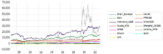
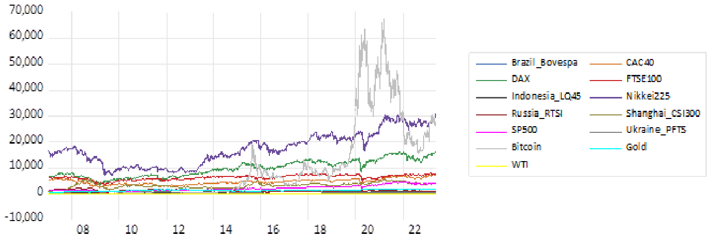
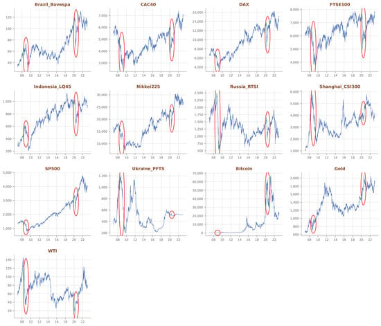
The variation in index series and returns over the study period is presented in Figure 1, Figure 2 and Figure 3, respectively. We observe that daily returns are volatile throughout the entire analysis period, particularly at the onset of various crises, especially during the subprime crisis, the crises caused by the COVID-19 pandemic in China, and finally, the Ukraine-Russia crisis. Moreover, it highlights the presence of volatility clustering in each return series. Furthermore, from the descriptive statistics provided in Table 1 and the distributional characteristics of the return series, we observe that all the averages were positive, except for Russia, which shows an average of −1%. The oil market recorded the lowest average of (0.052%), followed by the Ukrainian market with an average return of (0.056%). In contrast, Bitcoin posted the highest return average of (22.19%), followed by the Chinese market with the value of (3.1%).

Figure 1. Graphic of the evolution of index performance over time.

Figure 2. Multiple graphs of index performance trends.

Figure 3. Graph of return trends.

Table 1. Descriptive Statistics and Stochastic Properties of Return Series.

	R_BRAZIL	R_CHIN	R_GER	R_FR	R_INDO	R_JAP	R_RUSSIA	R_UK	R_UKR	R_USA	R_WTI	R_GOLD	R_BTC
Mean	0.026305	0.031030	0.021346	0.006288	0.029536	0.014550	−0.010236	0.005696	0.008863	0.027632	0.005257	0.025919	0.221899
Median	0.063403	0.072339	0.075890	0.045341	0.072849	0.060848	0.087870	0.052255	0.000000	0.069304	0.004953	0.033794	0.117720
Maximum	13.67861	8.930877	10.79747	10.59456	13.90798	13.23458	23.20443	24.43164	10.95720	72.25412	8.588967	147.4180	147.4190
Minimum	−15.99303	−9.695168	−13.59486	−13.09835	−12.62842	−12.11103	−48.29211	−11.51243	−15.18317	−12.76521	−132.4217	−9.810481	−84.88287
Std. Dev.	1.735553	1.670138	1.385755	1.409285	1.534716	1.466183	2.278153	1.180625	1.522245	1.285850	3.579076	1.111051	5.367616
Skewness	−0.421652	−0.553413	−0.197389	−0.258207	−0.358747	−0.436098	−2.478415	−0.418771	0.936722	−0.511086	−10.04911	−0.260515	4.182580
Kurtosis	12.36134	7.024679	10.81090	10.90082	11.43802	10.69048	61.27601	7.73222	33.55052	14.99374	493.4131	8.854971	173.7915
Jarque-Bera	15,460.52	3049.043	10,704.04	10,970.68	12,550.13	10,483.23	598,616.2	16,698.09	163,947.7	25,360.90	42,159.005	6046.628	5,116,948
Probability	0.000000	0.000000	0.000000	0.000000	0.000000	0.000000	0.000000	0.000000	0.000000	0.000000	0.000000	0.000000	0.000000
Observations	4200	4200	4200	4200	4200	4200	4200	4200	4200	4200	4200	4200	4200
Q(12)	38.688 ***	43.979 ***	9.878	32.392 ***	39.213 ***	15.76	17.124	47.489 ***	306.1 ***	120.4 ***	380.01 ***	24.405 **	322.77 ***
Q2(12)	1182.4 ***	1708.9 ***	1724 ***	1995 ***	2060 ***	3804 ***	370.43 ***	2743.2 ***	379.35	4997.9 ***	481.22 ***	562.31 ***	1077.2 ***

Notes: This table presents key statistics on daily returns over the period from 2 January 2007, to 29 May 2023. Q(12) et Q²(12) represent the Ljung–Box statistics for 12th-order serial correlation of returns and squared returns, respectively. **, and *** denote rejection of the null hypothesis of normality or absence of autocorrelation at the 5%, and 1% significance levels, respectively.

Our statistical results, as illustrated in the table, indicate that the historical volatility, measured by the standard deviation, places Bitcoin as the riskiest asset at 5.365%, followed by oil at 3.579%. In contrast, gold shows the lowest volatility at 1.11%. Additionally, we observe that all return series exhibit a negative skewness, except for the Ukrainian market index and Bitcoin. This suggests that both the Ukrainian market index and Bitcoin have experienced more negative shocks than positive ones during our observation period, indicating that they are asymmetrical markets in terms of their return distribution.

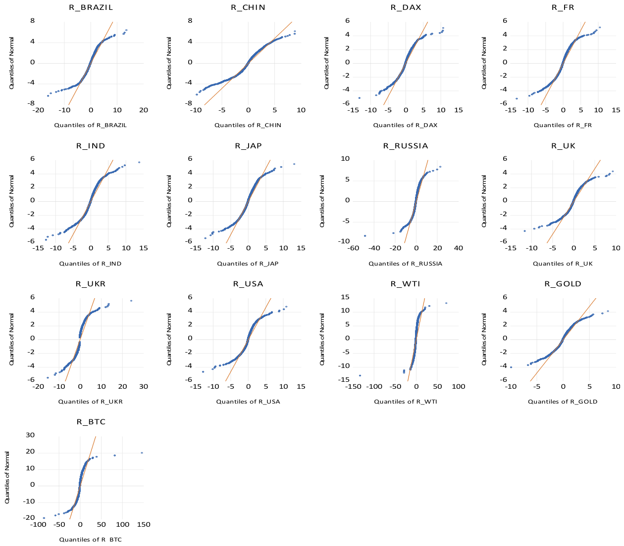
Most importantly, all markets exhibit a kurtosis greater than 3, indicating a high likelihood of large shocks, which suggests fat-tailed distributions and the presence of dependence on extreme values. To account for the existence of these fat-tails, we assume that the innovations follow a Student’s t-distribution. In fact, the Jacque-Bera test allows us to reject the hypothesis of normal distributions for the series under study, as do the QQ-plots of returns compared with the normal distribution (Figure 4).

Figure 4. QQ plots of returns compared with the normal distribution.

In addition, the Ljung–Box Q-statistics of order 12 for both raw returns and squared returns indicate the presence of significant autocorrelation, particularly for the squared returns across all series. This confirms the rejection of the null hypothesis of no autocorrelation in the squared return series. This statistical result suggests the presence of ARCH effects in our return series.

To assess the stationarity of the return series, we employed the Augmented Dickey–Fuller (ADF) test. The results, shown in Table 2, indicate that all return series are integrated of order 0 (I(0)), confirming their stationarity at the level.

Table 2. ADF Test and ARCH-LM Test for Heteroskedasticity.

	ADF Test in Levels	ARCH-LM(20)
Bitcoin	−25.100 ***,b	86.035 ***
Brazil	−68.726 ***,a	203.56 ***
Chine	−63.186 ***,a	99.025 ***
France	−66.704 ***,a	199.58 ***
Germany	−64.985 ***,a	182.53 ***
Indonesia	−60.595 ***,a	154,09 ***
Japan	−67.006 ***,a	123.54 ***
Oil	−27.742 ***,a	78.206 ***
Gold	−64.516 ***,a	77.303 ***
Russia	−63.137 ***,a	104.78 ***
UK	−66.837 ***,a	47.581 ***
Ukraine	−51.402 ***,a	111.07 ***
USA	−73.733 ***,a	175.23 ***

Notes: ADF denotes the Augmented Dickey–Fuller test. ^a: denotes Model 1 (without constant or trend); ^b: denotes Model 2 (with constant only). ARCH-LM is the Lagrange Multiplier test for autoregressive conditional heteroskedasticity. *** indicates rejection of the null hypothesis at the 1% significance level.

Furthermore, the results of the Lagrange multiplier test for ARCH heteroskedasticity, also presented in Table 2, confirm the presence of ARCH effects in the return data, thereby supporting our decision to adopt the GARCH approach.

4.2. GARCH Model Estimation Results

Before employing copula functions to measure the degree of interdependence among the variables, it is essential to select the most appropriate specifications for modeling conditional heteroscedasticity, as the kurtosis results in Table 1 suggest that a normal distribution is not suitable. To address this, univariate GARCH models with various error term distributions ${\mathsf{\epsilon }}_{\mathbf{t}}$ are applied to the return data and compared using standard information criteria such as the Akaike Information Criterion (AIC), the Schwarz Information Criterion (SIC), and the Log-Likelihood statistics.

According to Bollerslev (1986), models that best account for issues of conditional heteroscedasticity and autocorrelation for a time series $r_t$ are defined as the GARCH(1,1) model, specified as follows:

$$\begin{array}{c}\begin{array}{c}{r}_t=c+\varphi r_{t-1}+{\epsilon }_t\\ \mathrm{w}\mathrm{i}\mathrm{t}\mathrm{h} {\epsilon }_t={\sigma }_t{z}_t\end{array}\\ \mathrm{a}\mathrm{n}\mathrm{d} {\sigma }_t^2={\alpha }_0+{\alpha }_1{\epsilon }_{t-1}^2+{\beta }_1{\sigma }_{t-1}^2\end{array}$$

(15)

where $r_{t-1}$ denotes the first lag of returns and $\varphi$ is the autoregressive coefficient, and $z_t$ is $iid(\mathrm{0,1})$.

The results presented in Table 3 indicate that GARCH(1,1) models with an asymmetric Student’s t distribution are suitable for all return series, except for those of China, Germany, and Singapore, which follow a GARCH(1,1) model with generalized error distribution (GED).

Table 3. Estimation of Univariate GARCH Models Over the Entire Period.

	Mean Equation		Variance Equation			Dist. (DOF)	Information Criteria
	C	$\mathsf{\varphi }$	${\mathsf{\alpha }}_0$	${\mathsf{\alpha }}_1$	${\mathsf{\beta }}_1$		Dist.	AIC	SIC
Bitcoin	0.161 ***	−0.039 ***	0.423 ***	0.114 ***	0.830 ***	2.519 ***	t-stud	5.224	5.233
	(0.0332)	(0.0144)	(0.1095)	(0.0234)	(0.0114)	(0.1377)
Brazil	0.066 ***	−0.027 *	0.065 ***	0.073 ***	0.899 ***	9.132	t-stud	3.621	3.630
	(0.0203)	(0.0216)	(0.0134)	(0.0087)	(0.0115)	(1.0014)
Chine	0.052 ***	0.0045	0.012 ***	0.063 ***	0.933 ***	1.248 ***	GED	3.503	3.512
	(0.0166)	(0.0146)	(0.0041)	(0.0069)	(0.0065)	(0.0347)
France	0.074 ***	−0.029 **	0.028 ***	0.125 ***	0.868 ***	5.573 ***	t-stud	3.122	3.131
	(0.0144)	(0.0164)	(0.0062)	(0.0130)	(0.0123)	(0.4983)
Germany	0.086 ***	−0.031 **	0.032 ***	0.104 ***	0.880 ***	1.253 ***	GED	3.122	3.131
	(0.0139)	(0.0151)	(0.0068)	(0.0118)	(0.0129)	(0.0358)
Indonisia	0.069 ***	−0.014	0.045 ***	0.110 ***	0.871 ***	5.763 ***	t-stud	3.278	3.287
	(0.0161)	(0.0159)	(0.0088)	(0.0117)	(0.0121)	(0.5082)
Japan	0.074 ***	−0.030 *	0.033 ***	0.102 ***	0.884 ***	6.768 ***	t-stud	3.261	3.270
	(0.0163)	(0.0163)	(0.0076)	(0.0104)	(0.0113)	(0.7341)
Oil	0.082 ***	−0.022	0.114 ***	0.116 ***	0.868 ***	6.386 ***	t-stud	4.326	4.335
	(0.0266)	(0.0159)	(0.0216)	(0.0113)	(0.0110)	(0.5148)
Or	0.043 ***	−0.030 **	0.005 ***	0.032 ***	0.964 ***	4.060 ***	t-stud	2.774	2.783
	(0.0124)	(0.0146)	(0.0022)	(0.0049)	(0.0049)	(0.2972)
Russia	0.079 ***	0.045 ***	0.045 ***	0.078 ***	0.910 ***	5.794 ***	t-stud	3.860	3.869
	(0.0226)	(0.0157)	(0.0099)	(0.0083)	(0.0087)	(0.4107)
UK	0.048 ***	−0.020	0.026 ***	0.130 ***	0.854 ***	6.058 ***	t-stud	2.718	2.727
	(0.0120)	(0.0164)	(0.0051)	(0.0135)	(0.0135)	(0.6094)
Ukraine	−0.036 ***	0.117 ***	0.001 ***	0.053 ***	0.919 ***	-	Norm	2.949	2.956
	(0.0065)	(0.0174)	(6.42 × 10−5)	(0.0018)	(0.0018)
USA	0.090 ***	−0.061 ***	0.015 ***	0.147 ***	0.855 ***	5.231	t-stud	2.694	2.703
	(0.0105)	(0.0166)	(0.0034)	(0.0145)	(0.0123)	(0.4572)

Notes: This table summarizes the results of the GARCH estimation. The values in parentheses represent the standard errors of the parameters. Dist. denotes the selected error distribution. DOF stands for Degrees of Freedom of the following distribution. *, **, *** indicate significance levels of 10%, 5%, and 1%, respectively.

It is also noteworthy that for all series, the parameter β is around 0.9 and highly significant, except for the gold market. This result indicates that conditional volatility depends on past volatility and exhibits a high degree of persistence over time. Moreover, the total persistence degree, α + β < 1, implies that our GARCH models are all valid. However, since it is very close to 1, this suggests that the markets are quite volatile.

More specifically, another objective of this study is to investigate whether the coronavirus crisis caused a surge in correlations across markets, highlighting the contagion effect.

To identify a potential structural break associated with the COVID-19 outbreak, we employed the Breakpoint Unit Root Test (ADF-type) available in EViews 12. This procedure belongs to the family of endogenous structural break unit root tests developed in the tradition of Perron (1989) and Zivot and Andrews (1992). It searches over potential break dates and identifies the breakpoint associated with the most significant Augmented Dickey–Fuller statistic. The test indicated a significant structural break on 20 March 2020, for the Chinese market index. To validate this result, we additionally applied the Chow Breakpoint Test at the identified date.

This date is economically meaningful: it coincides with the period when global governments began implementing large-scale containment measures following the WHO pandemic declaration on 11 March 2020, triggering an abrupt and simultaneous repricing of risk across global financial markets. The end of the crisis sub-period is set at 29 May 2023, which corresponds to the end of our dataset and aligns with the progressive lifting of pandemic-era restrictions and the stabilization of financial conditions. This crisis window (20 March 2020–29 May 2023) is consistent with the time frames used in recent contagion studies (e.g., Akhtaruzzaman et al., 2021; Umar et al., 2022), which confirm that the pandemic’s financial effects extended well beyond the initial shock phase. The pre-crisis (calm) period spans from 2 January 2007 to 19 March 2020, capturing multiple economic cycles, including the Global Financial Crisis of 2008, thus providing a rich comparative baseline.

The results are shown in Table 4.

Table 4. Breakpoint tests on the Chinese markets.

Chow Breakpoint Test	Unit Root Test for Breakpoint
Break Date: 20 March 2020
F-statistic = 15.71696 (0.0042)	t-statistic = −49.1002
Wald statistic = 20.1552 (0.054)	p-value = 0.000

Notes: The Breakpoint Unit Root Test (ADF-type) is reported solely to identify the endogenous structural break date. In this study, it is not used as a conventional unit root test to assess the stationarity of the return series, which has already been examined using the standard ADF test reported in Table 2. (.) The values in parentheses are the critical probabilities.

After obtaining this significant finding, we need to find the marginal distribution that best describes each market around the coronavirus crisis. The results of this analysis are shown in Table 5 and Table 6. We note that in the calm period, the results are quite similar to what we observed for the whole period, in the case of gold, where the most appropriate is the normal distribution. For the crisis period, we find that most markets follow the Student’s t-distribution, while China, Germany, and Japan follow the generalized error distribution (GED).

Table 5. Estimation of Univariate GARCH Models During the Calm Period.

	Mean Equation		Variance Equation			Dist. (DOF)	Information Criteria
	C	$\mathsf{\varphi }$	${\mathsf{\alpha }}_0$	${\mathsf{\alpha }}_1$	${\mathsf{\beta }}_1$		Dist.	AIC	SIC
Bitcoin	0.151 ***	−0.069 ***	0.209 *	0.324 **	0.866 ***	2.410 ***	t-stud	5.062	5.078
	(0.0405)	(0.0195)	(0.1092)	(0.1274)	(0.0140)	(0.1418)
Brazil	0.059 **	−0.0124	0.043 **	0.042 ***	0.933 ***	9.099 ***	t-stud	3.383	3.399
	(0.0270)	(0.0230)	(0.0179)	(0.0106)	(0.0176)	(1.1493)
Chine	−0.027	0.025	0.029 ***	0.070 ***	0.909 ***	1.230 ***	GED	3.109	3.125
	(0.0210)	(0.0207)	(0.0090)	(0.0118)	(0.0134)	(0.0401)
France	0.075 ***	−0.026	0.042 ***	0.137 ***	0.137 ***	5.933 ***	t-stud	2.733	2.749
	(0.0176)	(0.0223)	(0.0117)	(0.0214)	(0.0214)	(0.6309)
Germany	0.080 ***	−0.002	0.025 ***	0.079 ***	0.900 ***	1.302 ***	GED	2.834	2.850
	(0.0185)	(0.0212)	(0.0080)	(0.0136)	(0.0159)	(0.0418)
Indonisia	0.054 ***	0.043 **	0.025 ***	0.125 ***	0.848 ***	5.644 ***	t-stud	2.439	2.456
	(0.0159)	(0.0221)	(0.007)	(0.0199)	(0.0210)	(0.5570)
Japan	0.063 ***	0.012	0.026 ***	0.078 ***	0.904 ***	1.331 ***	GED	3.011	3.027
	(0.0216)	(0.0220)	(0.0088)	(0.0129)	(0.0149)	(0.0415)
Oil	0.022	−0.045 **	0.03 **	0.073 ***	0.925 ***	6.398 ***	t-stud	4.015	4.031
	(0.0322)	(0.0219)	(0.0141)	(0.0118)	(0.0118)	(0.5638)
Or	−0.039 **	−0.175 ***	0.970 ***	0.265 ***	0.323 ***	-	Norm	3.502	3.515
	(0.0195)	(0.0363)	(0.0412)	(0.0245)	(0.0270)
Russia	0.072 ***	0.061 ***	0.027 ***	0.063 ***	0.929 ***	6.522 ***	t-stud	3.796	3.807
	(0.0252)	(0.0174)	(0.0082)	(0.0080)	(0.0085)	(0.5526)
UK	0.042 ***	−0.013	0.042 ***	0.139 ***	0.808 ***	7.033 ***	t-stud	2.331	2.347
	(0.0148)	(0.0235)	(0.0105)	(0.0227)	(0.0280)	(0.9171)
Ukraine	0.024 **	0.200 ***	0.009 ***	0.122 ***	0.817 ***	2.764 ***	t-stud	2.930	2.941
	(0.0121)	(0.0160)	(0.0031)	(0.0291)	(0.0115)	(0.1554)
USA	0.085 ***	−0.046 **	0.021 ***	0.172 ***	0.814 ***	4.782 ***	t-stud	2.156	2.172
	(0.0124)	(0.0233)	(0.0054)	(0.0241)	(0.0224)	(0.4490)

Notes: This table summarizes the GARCH estimation results. The values in parentheses represent the standard errors of the parameters. Dist. denotes the selected error distribution. DOF stands for Degrees of Freedom of the following distribution. *, **, *** indicate significance levels of 10%, 5%, and 1%, respectively.

Table 6. Estimation of Univariate GARCH Models During the Crisis Period from 20 March 2020 à 29 May 2023.

	Mean Equation		Variance Equation			Dist. (DOF)	Information Criteria
	C	$\mathsf{\varphi }$	${\mathsf{\alpha }}_0$	${\mathsf{\alpha }}_1$	${\mathsf{\beta }}_1$		Dist.	AIC	SIC
Bitcoin	−0.056	−0.060 **	0.463 **	0.079 **	0.886 ***	0.987 ***	GED	5.143	5.178
	(0.0748)	(0.0274)	(0.1194)	(0.0269)	(0.0402)	(0.0639)
Brazil	0.0533	−0.070 *	0.104 **	0.086 ***	0.867 ***	9.824 ***	t-stud	4.075	4.153
	(0.0441)	(0.0371)	(0.0406)	(0.0204)	(0.0291)	(0.0291)
Chine	0.010	−0.027	0.069 **	0.068 ***	0.8866 ***	6.715 ***	t-stud	3.385	3.449
	(0.0375)	(0.0376)	(0.0337)	(0.0222)	(0.0375)	(1.5044)
France	0.117 ***	−0.064 *	0.056 **	0.118 ***	0.851 ***	4.604 ***	t-stud	3.100	3.113
	(0.0327)	(0.0351)	(0.0222))	(0.0327)	(0.0345)	(0.8064)
Germany	0.088 ***	−0.097 ***	0.069 ***	0.122 ***	0.837 ***	1.120 ***	GED	3.181	3.216
	(0.0287)	(0.0317)	(0.026)	(0.0362)	(0.0398)	(0.0733
Indonisia	0.019	−0.111 ***	0.080 ***	0.146 ***	0.810 ***	6.044 ***	t-stud	3.139	3.173
	(0.0315)	(0.0382)	(0.0289)	(0.0349)	(0.0399)	(1.2443)
Japan	0.076 **	−0.026	0.097 **	0.106 ***	0.834 ***	1.488 ***	GED	3.161	3.226
	(0.0386)	(0.0362)	(0.0491)	(0.0314)	(0.0539)	(0.1169)
Oil	0.243 ***	0.024	0.417 ***	0.115 ***	0.817 ***	6.456	t-stud	5.004	5.069
	(0.0788)	(0.0371)	(0.1352)	(0.0326)	(0.0388)	(1.299)
Or	0.011	−0.066	0.140 **	0.021 **	0.835 ***	-	Norm	3.151	3.216
	(0.0338)	(0.0412)	(0.0637)	(0.0107)	(0.0706)
Russia	0.117 **	−0.013	0.143 ***	0.127 ***	0.852 ***	4.153 ***	GED	4.112	4.147
	(0.0518)	(0.0357)	(0.0529)	(0.0286)	(0.0278)	(0.5715)
UK	0.070 ***	−0.090**	0.046 **	0.152 ***	0.826 ***	4.035 ***	t-stud	2.803	2.838
	(0.0259)	(0.0359)	(0.0191)	(0.0414)	(0.0383)	(0.6694)
Ukraine	−3.5 × 10−28	−1. × 10−6 ***	1.1 × 10−8 ***	0.004 ***	0.576 ***	0.040 ***	GED	−62.55	−62.52
	(4.2 × 10−9)	(1.1 × 10−7)	(3.01 × 10−9)	(0.0011)	(0.0132)	(0.0001)
USA	0.109 ***	−0.059	0.036**	0.136 ***	0.844 ***	8.437 ***	t-stud	3.178	3.213
	(0.0336)	(0.0382)	(0.0147)	(0.0327)	(0.0324)	(2.1201)

Notes: This table summarizes the GARCH estimation results. The values in parentheses represent the standard errors of the parameters. Dist. denotes the selected error distribution. DOF stands for Degrees of Freedom of the following distribution. *, **, *** indicate significance at the 10%, 5%, and 1% levels, respectively.

Prior to estimating the copula parameters, we verify the adequacy of the GARCH(1,1) specifications by applying diagnostic tests on the standardized residuals. Specifically, we report the Ljung–Box statistics Q(12) for serial correlation in the standardized residuals, as well as the ARCH-LM(5) test for remaining conditional heteroscedasticity. The results, presented in Table 7, indicate that for all assets and sub-periods, the null hypotheses of no autocorrelation and no remaining ARCH effects cannot be rejected at the 5% significance level, confirming the overall adequacy of the GARCH(1,1) filter.

Table 7. Residual Diagnostic Tests on Standardized GARCH(1,1) Residuals.

	Full Period		Calm Period (Jan 2012–Mar 2020)		Crisis Period (Mar 2020–Apr 2021)
Asset	Q(12)	ARCH-LM(5)	Q(12)	ARCH-LM(5)	Q(12)	ARCH-LM(5)
China	17.251	4.132	18.230	4.038	13.492	5.489
France	11.918	3.350	12.904	4.673	15.037	3.716
Germany	10.973	1.625	16.531	2.672	13.388	2.205
USA	13.695	1.011	15.124	0.149	9.697	10.691
UK	17.418	5.442	16.064	4.911	12.046	2.024
Ukraine	14.782	2.187	15.224	1.726	10.736	4.408
Japan	12.336	3.772	8.750	1.868	8.964	1.352
Brazil	9.838	2.421	7.112	6.846	12.146	5.733
Indonesia	11.566	8.902	18.152	3.970	10.682	4.585
Russia	12.235	3.044	16.087	2.782	7.785	2.842
Bitcoin	18.723	2.518	14.475	2.405	4.939	2.675
Gold	15.896	2.023	17.078	4.136	11.404	4.515
Oil	14.221	2.341	16.545	2.643	9.260	2.344

Notes: Values reported as Statistics tests. Q(12) and Q²(12) are Ljung–Box statistics for serial correlation in standardized residuals. ARCH-LM(5) is the Lagrange Multiplier test for remaining ARCH effects.

Given the availability of GARCH model estimates, we now turn to the estimation of copula functions for each pair linking the Chinese market’s return with those of other markets. To do this, we take the vector of standardized residuals ${(x_{1t},x_{2t},\dots ,x_{nt})}_{t=1}^T$ from the GARCH models estimated above and transform it into a vector of uniform variables ${(u_{1t},u_{2t},\dots ,u_{nt})}_{t=1}^T$ using Empirical Cumulative Distribution Functions (EDCF).

Table 7 below summarizes the correlation coefficients for dependence based on Kendall’s tau and Spearman’s rho statistics between the returns of the Chinese market and those of other markets during three periods (calm period, crisis period, and overall period). For the overall period, both Kendall’s tau and Spearman’s rho statistics indicate a positive relationship for all pairs considered, except for the China–USA, China–Germany, and China–Gold pairs. These findings are generally supported by those from the normal period, albeit with higher values. However, during the crisis period, the coefficients show greater magnitude for most pairs, with some sign changes compared with the calm period. Notably, the correlation coefficients between China–Bitcoin and China–France have turned negative, while the dependence between China and Germany has become positive. Overall, co-movement is significantly higher during the crisis period.

The statistical values of the Spearman and Kendall correlation coefficients demonstrate that the degree of dependence between markets has been increasing due to the COVID-19 pandemic. This negatively impacts portfolio diversification opportunities, which are becoming increasingly limited. International financial markets tend to fluctuate during both volatile and calm periods. As shown in Table 8.

Table 8. Estimation of Spearman’s Correlation Coefficient and Kendall’s Tau between the Chinese Market’s Returns and Other Markets.

	Entire Period		Normal Period		Crisis Period
	Spearman	Kendall	Spearman	Kendall	Spearman	Kendall
China/Bitcoin	0.0026	0.0015	0.0095	0.0063	−0.0351	−0.0233
China/Brazil	0.0186	0.0124	0.0189	0.0128	0.0186	0.0117
China/France	0.0004	0.0004	0.0044	0.0032	−0.0183	−0.0138
China/Germany	−0.0154	−0.0102	−0.0196	−0.0132	0.0064	0.0044
China/Indonesia	0.0442	0.0298	0.0431	0.0292	0.0402	0.0261
China/Japan	0.0164	0.0111	0.0022	0.0014	0.0825	0.0561
China/Oil	0.0068	0.0046	0.0004	0.0003	0.0373	0.0249
China/Gold	−0.0079	−0.0053	−0.0060	−0.0041	−0.0167	−0.0113
China/Russia	0.0396	0.0268	0.0479	0.0324	0.0058	0.0037
China/UK	0.0167	0.0117	0.0112	0.0080	0.0428	0.0294
China/Ukraine	0.0487	0.0332	0.0556	0.0381	0.0338	0.0129
China/USA	−0.0097	−0.0063	−0.0001	−7.9 × 10−5	−0.0525	−0.0362

4.3. Estimation of Copula Parameters

Table 9 and Table 11 report the estimated parameters for the six copulas defined in Section 3.2.3 over the three periods: calm, crisis, and total. However, to identify the best-fitting copula for the data, we apply the goodness-of-fit test following the methodology of Genest et al. (2009), which is based on comparing the distance between the estimated and empirical copulas:

$${\mathbb{C}}_n=\sqrt{n}\left({\mathbb{C}}_n-{\mathbb{C}}_{\theta n}\right)$$

(16)

The test statistics are based on the Cramer–von Mises distance, defined as:

$$S_n=\int {\mathbb{C}}_n{\left(u\right)}^{2}d{C}_n(u)$$

(17)

Table 9. Estimation of Copula Parameters for the Entire Period.

	Normal	t-Student		Frank	Plackett	Gumbel	Clayton
Parameter	$\mathit{\rho }$	$\mathit{\theta }$	$\mathit{\gamma }$	θ	Θ	θ	Θ
China/Bitcoin	0.015 ***	0.0131 ***	7.44 ***	1.0429 ***	0.1749 ***	1.1154 ***	0.0164 ***
	(0.0004)	(0.0009)	(2.0368)	(0.0165)	(0.0247)	(0.0083)	(0.0087)
China/Brazil	0.0361 ***	0.0211 ***	14.57 ***	0.028	0.998 ***	1.0219 ***	0.0293 ***
	(0.0043)	(0.0088)	(2.0458)	(0.107)	(0.057)	(0.0284)	(0.0084)
China/France	0.0361 ***	−0.0453 ***	8.16 ***	1.085 ***	0.162 ***	1.027 ***	0.0717 ***
	(0.0049)	(0.0012)	(1.4120)	(0.015)	(0.022)	(0.5025)	(0.0229)
China/Germany	−0.02 ***	−0.0195 ***	13.12 ***	−1.101 ***	0.138 ***	1.012 ***	0.0429 ***
	(0.0058)	(0.0006)	(1.0458)	(0.014)	(0.0297)	(0.0935)	(0.0099)
China/Indonesia	0.0244 ***	−0.0009 ***	9.50 ***	−1.01 ***	−0.006 ***	1.0084 ***	0.0379 ***
	(0.0058)	(0.0008)	(1.4580)	(0.0123)	(0.0191)	(0.0101)	(0.0086)
China/Japan	−0.0244 ***	−0.0311 ***	5.82 ***	−1.165 ***	0.279 ***	1.0219 ***	0.0718 ***
	(0.0018)	(0.0008)	(1.0754)	(0.0126)	(0.0148)	(0.1025)	(0.0102)
China/Oil	0.0197 ***	−0.0016 ***	11.34 ***	−1.25 ***	−0.0047 ***	1.120 ***	0.0128 ***
	(0.0018)	(0.0009)	(1.0254)	(0.0093)	(0.0012)	(0.8699)	(0.0054)
China/Gold	0.125 ***	−0.0548 ***	24.15 ***	−1.015 ***	−0.223 ***	1.225 ***	0.0498 ***
	(0.0034)	(0.0042)	(2.0684)	(0.1223)	(0.0025)	(0.0254)	(0.0022)
China/Russia	0.0164 ***	0.0143 ***	8.14 ***	1.141 ***	0.1914 ***	1.0015 ***	0.01789 ***
	(0.0004)	(0.0010)	(2.2284)	(0.018)	(0.027)	(0.0091)	(0.0095)
China/UK	0.0525 ***	0.0557 ***	3.41 ***	−0.036 ***	0.893 ***	1.0061 ***	0.0228 ***
	(0.0071)	(0.0048)	(1.1102)	(0.0123)	(0.0521)	(0.0589)	(0.0012)
China/Ukraine	0.0084 ***	0.0107 ***	5.124 ***	−0.0871 **	−0.0147 ***	0.8975 ***	0.0047 ***
	(0.0003)	(0.0045)	(1.1154)	(0.0045)	(0.0078)	(0.0105)	(0.0004)
China/USA	0.0191 ***	0.0215 ***	12.22 ***	1.008 ***	0.153 ***	1.0100 ***	0.0133 ***
	(0.0015)	(0.0011)	(2.0151)	(0.0114)	(0.023)	(0.0877)	(0.0049)

Notes: The values in parentheses represent the standard deviations of the parameters. **, *** Indicate the significance level at 5% and 1%, respectively.

The copula that best fits the sample is the one that minimizes this distance. Table 10 provides the values of this distance measure and shows that the t-Student copula is the most suitable for modeling the conditional dependence structure of the markets in our sample over the entire period, except for gold and Bitcoin, which follow a Gumbel copula—an asymmetrical copula skewed to the right.

Table 10. Distance Measure Between Each Parametric Copula and the Empirical Copula, along with the Goodness-of-Fit Test for the Entire Period.

	Normal	t-Student	Frank	Plackett	Gumbel	Clayton
China/Bitcoin	0.012 (0.216)	0.006 (0.156)	0.022 (0.105)	0.018 (0.209)	0.0019 (0.458)	0.020 (0.113)
China/Brazil	0.034 (0.211)	0.033 (0.218)	0.034 (0.211)	0.035 0.208)	0.037 (0.198)	0.039 (0.155)
China/France	0.030 (0.305)	0.025 (0.389)	0.028 (0.325)	0.029 (0.311)	0.030 (0.305)	0.026 (0.366)
China/Germany	0.025 (0.211)	0.021 (0.287)	0.024 (0.220)	0.023 (0.254)	0.024 (0.220)	0.027 (0.191)
China/Indonesia	0.022 (0.189))	0.020 (0.258)	0.022 (0.189)	0.025 (0.165)	0.033 (0.103)	0.023 (0.181)
China/Japan	0.043 (0.194)	0.036 (0.271)	0.042 (0.211)	0.040 (0.229)	0.045 (0.188)	0.037 (0.258)
China/Oil	0.044 (0.138)	0.039 (0.154)	0.051 (0.108)	0.040 (0.150)	0.049 (0.122)	0.041 (0.145)
China/Gold	0.011 (0.197)	0.013 (0.192)	0.010 (0.202)	0.022 (0.176)	0.008 (0.208)	0.015 (0.184)
China/Russia	0.023 (0.436)	0.022 (0.441)	0.023 (0.436)	0.024 (0.429)	0.026 (0.409)	0.030 (0.386)
China/UK	0.045 (0.219)	0.022 (0.489)	0.044 (0.233)	0.051 (0.195)	0.067 (0.143)	0.071 (0.110)
China/Ukraine	0.075 (0.115)	0.0015 (0.334)	0.044 (0.104)	0.052 (0.119)	0.047 (0.1078)	0.0094 (0.2105)
China/USA	0.028 (0.355)	0.024 (0.413)	0.027 (0.376)	0.028 (0.355)	0.030 (0.294)	0.033 (0.246)

Notes: The values in parentheses represent the p-values of the goodness-of-fit test, based on the multiplier approach described by Kojadinovic and Yan (2011). A higher p-value indicates that the distance between the empirical and theoretical copula is the smallest, and thus the corresponding copula is the best fit.

These Student copulas also provide evidence of significant and symmetric tail dependence for all the pairs considered. This finding has been confirmed by several analysts, who demonstrated that the Student copula is more effective in capturing extreme dependencies compared with a Gaussian copula. However, only the indices of the gold and Bitcoin markets exhibit asymmetrical behavior, with a concentration on the extreme right tail, throughout the sample period.

A second analysis will be essential during the crisis period to determine whether the coronavirus pandemic has impacted the stochastic properties of certain markets. The results of this analysis are presented in the following Table 11 and Table 12.

Table 11. Estimation of Copula Parameters During the Crisis Period.

	Normal	t-Student		Frank	Plackett	Gumbel	Clayton
Parameter	$\mathit{\rho }$	$\mathit{\theta }$	$\mathit{\gamma }$	θ	Θ	θ	Θ
China/Bitcoin	0.113 ***	0.142 ***	11.25 ***	1.334 ***	0.254 ***	1.215 ***	0.146 ***
	(0.0034)	(0.0119)	(2.0145)	(0.0442)	(0.0154)	(0.0154)	(0.0108)
China/Brazil	0.124 ***	0.111 ***	9.79 ***	0.987 ***	0.546 ***	1.309 ***	0.491 ***
	(0.0443)	(0.0188)	(2.6658)	(0.147)	(0.154)	(0.1174)	(0.0145)
China/France	0.121 ***	−0.954 ***	12.56 ***	1.102 ***	0.445 ***	1.354 ***	0.413 ***
	(0.0159)	(0.0954)	(2.548)	(0.945)	(0.0991)	(0.1254)	(0.0664)
China/Germany	−0.154 ***	−0.0195 ***	13.12 ***	−1.101 ***	0.138 ***	1.012 ***	0.0429 ***
	(0.0058)	(0.0006)	(1.0458)	(0.014)	(0.0297)	(0.0935)	(0.0099)
China/Indonesia	0.354 ***	−0.0154 ***	22.35 ***	−1.245 ***	−0.095 ***	1.1245 ***	0.735 ***
	(0.0118)	(0.0044)	(3.258)	(0.0772)	(0.0054)	(0.0975)	(0.0032)
China/Japan	−0.124 ***	−0.544 ***	13.28 ***	−1.443 ***	0.664 ***	1.452 ***	0.245 ***
	(0.0010)	(0.0098)	(4.0459)	(0.0185)	(0.0228)	(0.1154)	(0.0854)
China/Oil	0.114 ***	−0.1205 ***	22.56 ***	−1.345 ***	−0.178 ***	1.338 ***	0.645 ***
	(0.0745)	(0.0105)	(5.4681)	(0.0112)	(0.0442)	(0.0786)	(0.0122)
China/Gold	0.207 ***	−0.145 ***	13.585 ***	−1.235 ***	−0.875 ***	1.334 ***	0.1245 ***
	(0.0077)	(0.0108)	(1.985)	(0.0548)	(0.0012)	(0.0457)	(0.0452)
China/Russia	0.384 ***	0.433 ***	16.58 ***	1.335 ***	0.1914 ***	1.215 ***	0.154 ***
	(0.0081)	(0.0054)	(4.587)	(0.2255)	(0.0087)	(0.0087)	(0.0122)
China/UK	0.112 ***	0.215 ***	7.458 ***	−0.454 ***	0.775 ***	1.210 ***	0.145 ***
	(0.0045)	(0.0124)	(2.312)	(0.0814)	(0.0354)	(0.0147)	(0.0109)
China/Ukraine	0.207 ***	−0.145 ***	13.585 ***	−1.235 ***	−0.875 ***	1.334 ***	0.1245 ***
	(0.0077)	(0.0108)	(1.985)	(0.0548)	(0.0012)	(0.0457)	(0.0452)
China/USA	0.137 ***	0.188 ***	21.57 ***	1.345 ***	0.478 ***	1.227 ***	0.389 ***
	(0.0015)	(0.0011)	(6.789)	(0.0449)	(0.0097)	(0.0149)	(0.0010)

Notes: The values in parentheses represent the standard deviations of the parameters. *** indicate significance levels of 1%, respectively.

Table 12. Measurement of the Distance Between Each Parametric Copula and the Empirical Copula, along with the Goodness-of-Fit Test for the Crisis Period.

	Normal	t-Student	Franck	Plackett	Gumbel	Clayton
China/Bitcoin	0.015048	0.023826	0.027588	0.022572	0.007524	0.02508
	(0.270864)	(0.198132)	(0.13167)	(0.262086)	(0.571824)	(0.141702)
China/Brazil	0.042636	0.040398	0.042636	0.04389	0.041382	0.048906
	(0.264594)	(0.448292)	(0.264594)	(0.260832)	(0.273372)	(0.19437)
China/France	0.03762	0.03762	0.035112	0.036366	0.03135	0.032604
	(0.38247)	(0.38247)	(0.40755)	(0.389994)	(0.487806)	(0.458964)
China/Germany	0.03135	0.010096	0.030096	0.028842	0.026334	0.033858
	(0.264594)	(0.37588)	(0.27588)	(0.318516)	(0.359898)	(0.239514)
China/Indonesia	0.027588	0.021382	0.027588	0.03135	0.02108	0.028842
	(0.237006)	(0.429162)	(0.237006)	(0.20691)	(0.433532)	(0.226974)
China/Japan	0.053922	0.03643	0.052668	0.05016	0.025144	0.046398
	(0.243276)	(0.435752)	(0.264594)	(0.287166)	(0.439834)	(0.323532)
China/Oil	0.055176	0.041446	0.063954	0.05016	0.048906	0.051414
	(0.173052)	(0.252988)	(0.135432)	(0.1881)	(0.193116)	(0.18183)
China/Gold	0.013794	0.020032	0.01254	0.027588	0.011302	0.01881
	(0.247038)	(0.260832)	(0.253308)	(0.220704)	(0.280768)	(0.230736)
China/Russia	0.028842	0.022604	0.028842	0.030096	0.027588	0.03762
	(0.546744)	(0.572886)	(0.546744)	(0.537966)	(0.553014)	(0.484044)
China/UK	0.05643	0.024018	0.055176	0.063954	0.027588	0.089034
	(0.274626)	(0.679322)	(0.292182)	(0.24453)	(0.613206)	(0.13794)
China/USA	0.035112	0.03762	0.033858	0.035112	0.030096	0.041382
	(0.44517)	(0.368676)	(0.471504)	(0.44517)	(0.517902)	(0.308484)

Notes: The values in parentheses represent the p-values from the goodness-of-fit test based on the multiplier approach described by Kojadinovic and Yan (2011). A higher p-value indicates that the distance between the empirical and theoretical copulas is smaller, suggesting that the corresponding copula is the best estimate.

Based on the results from the goodness-of-fit test performed during the crisis, there appears to be asymmetry in the USA, gold, France, Japan, Indonesia, and Bitcoin markets. The Gumbel copula is particularly useful to capture the dependence between these markets and the Chinese market, while illustrating an asymmetric feature of dependence, with extreme values concentrated mainly in the right tail. These findings demonstrate that the COVID-19 crisis has impacted stochastic properties in selected markets, similar to Liu et al. (2017). Liu et al. (2017) argue that copulas with time-varying parameters failed to capture potentially significant changes in the stochastic properties of the market’s returns. Copulas with time-varying parameters do not account for a potential time-varying dependence parameter with significant shifts within the copula family.

Indeed, asymmetric dependence for the returns of the aforementioned markets has been reported in previous studies. Rodriguez (2007) identified tail dependence in five East Asian countries during the Mexican and Asian crises. Similar findings were reported by Chen et al. (2014) for the Chinese market and by Ye et al. (2012) for four emerging Asian markets during the subprime crisis.

4.4. Measures of Dependence and Risk

The dependence measures to be studied will include the parameters of the appropriate copula, Kendall’s tau, Spearman’s rho, and the lower- and upper-tail dependence coefficients, to comprehensively understand the dependence structure of each pair of indices. We also estimate the value at risk for every pair of indexes so as to simulate and forecast the maximum risk. Such measures are summarized in Table 13 below.

Table 13. Dependence measures based on the t-Student Copula.

Couple	Copula Dependence Parameter	Degree of Freedom	Kendall’ Tau	Spearman’s Rho	Lower Tail Dependence	Upper Tail Dependence	VaR (95%)
China/Japan	−0.0311	5.82	−0.0198	−0.0296	0.0823	0.0823	1.958
China/France	−0.0453	8.16	−0.0288	−0.0432	0.0856	0.0856	1.805
China/Germany	0.0195	13.12	0.0124	0.0186	0.0798	0.0798	2.093
China/UK	0.0557	3.41	0.0354	0.0531	0.0644	0.0644	1.945
China/Oil	0.0964	21.1414	0.0189	0.0661	0.1393	0.1393	2.5922
China/Gold	−0.0889	N/A	−0.3155	−0.4476	0	0.1562	1.9436
China/Bitcoin	−0.0651	N/A	−0.3094	−0.4410	0	0.1482	1.9255
China/USA	−0.0215	12.22	−0.0136	−0.0205	0.0711	0.0711	2.131
China/Indonesia	0.1125	8.25	0.0244	0.0236	0.0758	0.0705	1.581
China/Russia	0.0143	8.14	0.0091	0.0136	0.0725	0.0725	2.021
China/Brazil	0.0009	9.50	−0.0005	0.0008	0.0757	0.0757	2.009

Note: The degrees-of-freedom parameter is only applicable to the Student’s t-copula. For pairs modeled by the Gumbel copula (China/Bitcoin and China/Gold), the corresponding entries are reported as “N/A”.

Results suggest that in the case of all index pairs, the dependency coefficient is positive but relatively low, and only for China/Bitcoin, China/France, China/Gold, and China/USA can it be seen as being negative and relatively weak. Such a low, positive value of dependency from results indicates an extremely low level of dependency. This would, in turn, imply that returns are moving in the same direction while China/Bitcoin, China/France, China/Gold, and China/USA move in opposite directions.

Kendall’s tau is significantly positive for most index pairs, except for the following pairs where it is negative: (China/Bitcoin), (China/France), (China/USA), and (China/Gold). This indicates that the probability of concordance is significantly higher (or lower, respectively) than the probability of discordance. Similarly, Spearman’s rho is also significantly positive (or negative, respectively), reflecting a clear rank correlation. The values of Kendall’s tau and Spearman’s rho for all index pairs are consistent with each other. Finally, the positive lower and upper tail dependence coefficients for all index pairs indicate the presence of extreme tail dependence. However, it is necessary to note that Tail dependence coefficients depend on the selected copula family. For the Student’s t-copula, lower- and upper-tail dependence coefficients are theoretically identical due to the symmetry of the copula. In contrast, the Gumbel copula exhibits only upper-tail dependence. For the Student’s t-copula, lower- and upper-tail dependence coefficients are identical and given by

$${\lambda }_L={\lambda }_U=2t_{\gamma +1}\left(-\sqrt{{\displaystyle \frac{\left(\gamma +1)(1-\theta \right)}{1+\theta }}}\right),$$

reflecting the symmetric tail dependence property of the copula. In contrast, for the Gumbel copula,

$${\lambda }_L=0,{\lambda }_U=2-2^{1/\theta },$$

implying upper-tail dependence only.

The estimation of value-at-risk (VaR) at the 95% significance level is conducted as follows: Each day, t, the model parameters are re-estimated, and the VaR is recalculated based on the last 500 available observations. This is done by adding the return of day t and dropping the return of day t-500 (rolling estimation). By comparing the out-of-sample VaR estimates with the corresponding realized returns, we can determine how many times a portfolio’s loss for a given pair exceeds the estimated VaR. The average VaR values for the different index pairs and quantiles are presented in Table 13 below.

Upon examining the results, it can be concluded that the VaR estimation method using the Copula-GARCH(1,1) model with either a t-Student or Gumbel distribution provides statistically acceptable results (neither overestimating nor underestimating risk) for the 95% quantile. The China/Oil pair shows the highest value-at-risk, followed by the China/USA portfolio. However, the China/Indonesia pair exhibits the lowest level of risk in terms of VaR.

VaR Backtesting

To formally assess the accuracy of our VaR estimates, we implement three complementary backtesting procedures over the full out-of-sample period (N = 1873 observations), following a rolling window of 500 observations.

First, the Kupiec (1995) unconditional coverage test examines whether the observed violation rate—defined as the proportion of days on which the realized portfolio loss exceeds the estimated VaR—is statistically consistent with the nominal level of 5%. The likelihood ratio statistic LR_uc is distributed as χ²(1) under the null hypothesis of correct coverage. Second, the Christoffersen (1998) conditional coverage test jointly examines unconditional coverage and the independence of violations over time, with the test statistic LR_cc distributed as χ²(2). Third, the Dynamic Quantile (DQ) test of Engle and Manganelli (2004) regresses the centered hit sequence on four of its own lags and the current VaR estimate, testing whether the VaR model captures all predictable variation in the violation process.

The results, presented in Table 14, indicate that the Kupiec test does not reject the null hypothesis of correct unconditional coverage for any of the ten portfolio pairs (all p-values > 0.05), confirming that the model produces an appropriate number of violations on average. The Christoffersen test further validates the independence of violations for nine out of ten pairs, except for the China/France pair (p = 0.003), which exhibits mild clustering of violations during the crisis period. Regarding the DQ test, several pairs display residual dependence in the hit sequence, a result that is consistent with the well-documented limitation of static copula frameworks in capturing time-varying dependence dynamics (Patton, 2006). Notwithstanding this limitation, the overall backtesting evidence supports the statistical adequacy of the Copula-GARCH(1,1) model for portfolio risk measurement at the 95% confidence level.

Table 14. VaR Backtesting Results—Kupiec, Christoffersen, and Dynamic Quantile Tests (α = 95%).

	Observed Violations			Kupiec (1995)		Christoffersen (1998)		Dynamic Quantile
Pair	N	Violations	Rate (%)	LR Stat	p-Value	LR Stat	p-Value	DQ Stat	p-Value	Interpretation
China/Japan	1873	86	4.59%	0.675	0.411	0.284	0.594	20.955	0.002	Conditional fail
China/France	1873	88	4.70%	0.366	0.545	8.972	0.003	34.104	0.000	Invalid
China/Germany	1873	95	5.07%	0.020	0.886	0.007	0.932	38.484	0.000	Conditional fail
China/UK	1873	88	4.70%	0.366	0.545	1.840	0.175	26.984	0.000	Conditional fail
China/Oil	1873	76	4.06%	3.732	0.053	0.271	0.603	17.983	0.006	Conditional fail
China/Gold	1873	91	4.86%	0.080	0.778	0.095	0.758	10.712	0.098	Valid
China/Bitcoin	1873	97	5.18%	0.125	0.724	0.778	0.378	6.53	0.367	Valid
China/USA	1873	91	4.86%	0.080	0.778	0.564	0.453	27.124	0.000	Conditional fail
China/Indonesia	1873	83	4.43%	1.323	0.250	0.506	0.477	7.66	0.264	Valid
China/Brazil	1873	97	5.18%	0.125	0.724	1.047	0.306	27.786	0.000	Conditional fail
China/Ukraine	1873	93	5.02%	0.165	0.451	1.604	0.189	25.451	0.000	Conditional fail
China/Russia	1873	90	4.63%	0.341	0.625	0.812	0.339	27.214	0.000	Conditional fail

Notes: N = number of out-of-sample observations. Violations = number of times the realized portfolio loss exceeds the estimated VaR at 95%. Kupiec (1995) LR statistic tests unconditional coverage (H0: actual violation rate = 5%). Christoffersen (1998) LR statistic tests conditional coverage and independence of violations. Dynamic Quantile (DQ) test follows Engle and Manganelli (2004) with 4 lags. Green p-values indicate non-rejection of H0 at 5% (valid VaR model); red indicates rejection. VaR estimated using a rolling window of 500 observations with the Copula-GARCH(1,1) model.

5. Robustness Analysis Using the Wavelet Method

To conduct the robustness analysis, we employed the wavelet approach developed by Grinsted et al. (2004), which aims to detect co-movements between time series across different investment horizons. The main advantage of wavelet analysis compared with standard econometric time series modeling methods is its ability to capture slow and persistent co-movements, providing a more nuanced understanding of the interdependence between two time series in both the time and frequency domains.

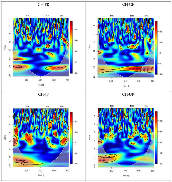
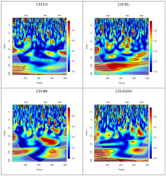
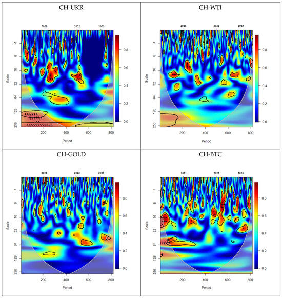
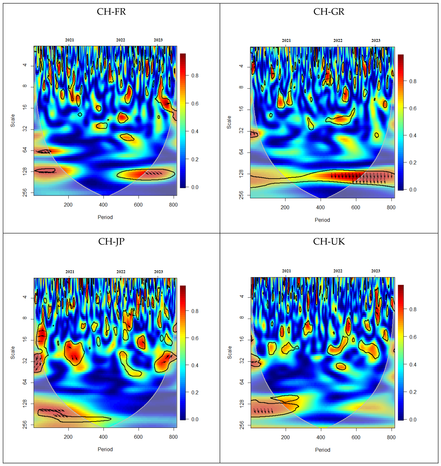
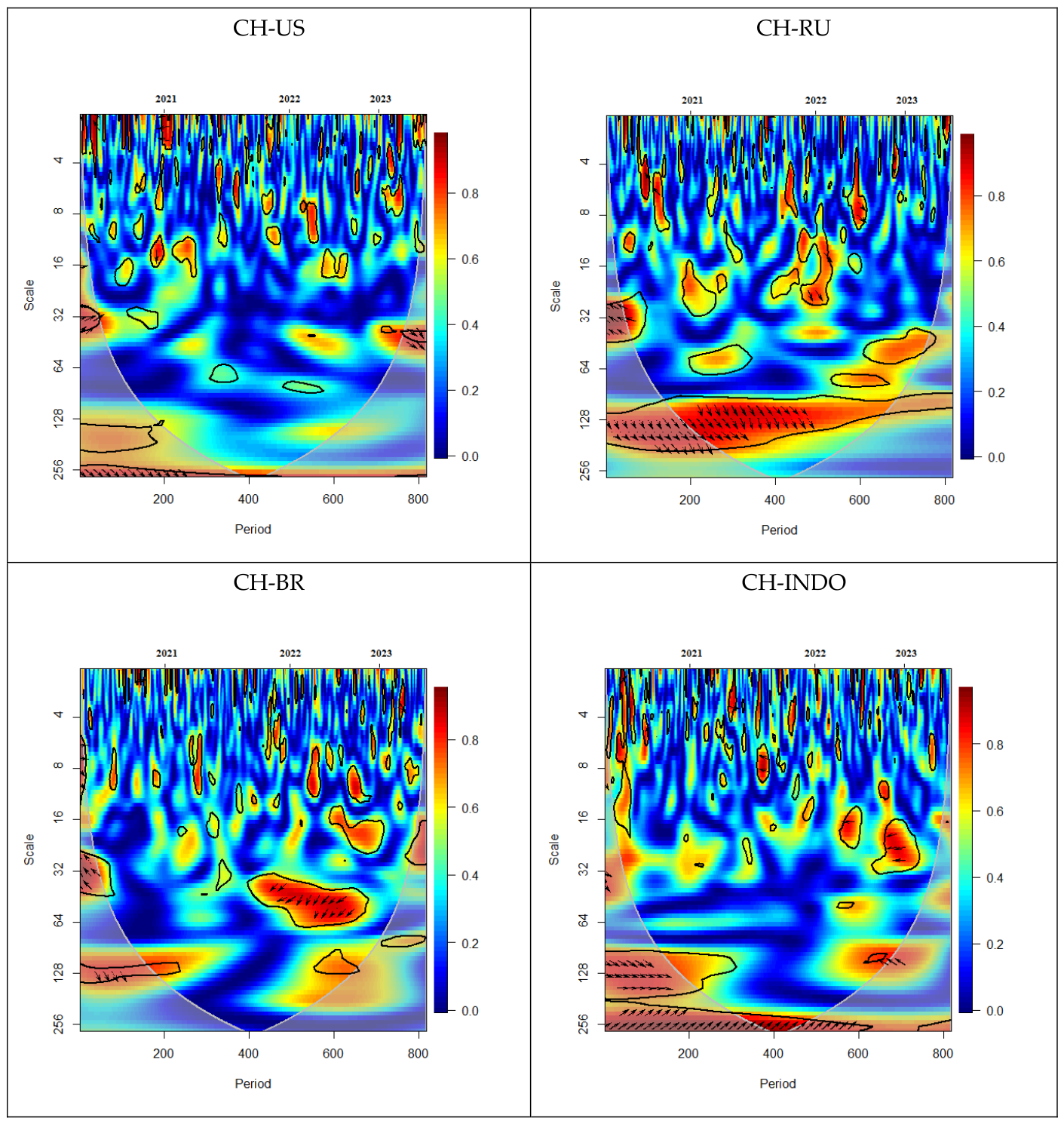
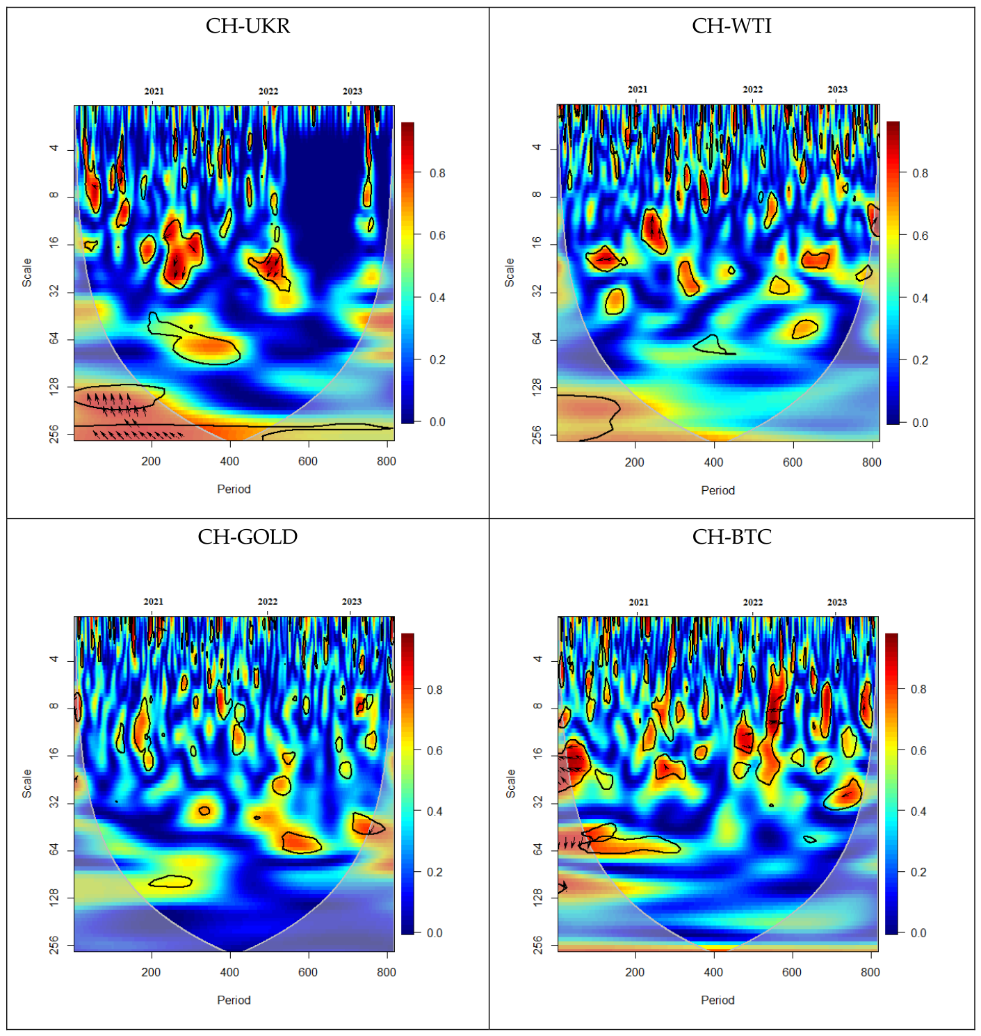
In the estimated wavelet coherence diagrams, the black contour indicates the 5% significance level; the warmer red color represents areas of strong co-movement, while the cooler blue color indicates areas of weak co-movement. The arrows illustrate the direction of interdependence and causal relationships. If the arrows point to the right, this suggests that the two series are positively correlated. Conversely, when the arrows point to the left, it indicates that the two variables are negatively correlated. Arrows pointing upward to the right and downward to the left (↗↙) suggest that the first variable causes the second, whereas arrows pointing downward to the right and upward to the left (↘↖) indicate that the second variable causes the first. Also, in all wavelet coherence figures, the horizontal axis reports the observation number within the sample period, while the vertical axis indicates the frequency scale.

Overall, (see Figure 5) we observe some substantial co-movements upon first visual examination between each pair and many small clusters, suggesting strong dependence in the beginning, middle, and end of the sampling period with entire ranges: specifically, medium to long horizons of 16 over 1024 frequencies.

Figure 5. Wavelet coherence between the Chinese stock market and: CH-FR (France), CH-GR (Germany), CH-JP (Japan), CH-UK (United Kingdom), CH-US (USA), CH-RU (Russia), CH-BR (Brazil), CH-INDO (Indonesia), CH-UKR (Ukraine), CH-WTI (crude oil), CH-GOLD (gold), CH-BTC (Bitcoin). Warmer colors (red) indicate stronger co-movement, while cooler colors (blue) indicate weaker co-movement; the black contour marks the 5% significance level; arrows indicate the direction and phase (lead/lag) relationship as described in the text.

From the very beginning of the COVID-19 crisis until the conclusion of the sample period, we can see a couple of small areas of strong positive and negative co-movement between the Chinese market and other developed and emerging markets where the causality relationship is bidirectional. However, during the period of 2007 until late 2010, we see strong negative co-movement between the Chinese market and crude oil over a 256-period horizon, and the Chinese market is dominant. Conversely, for the period 2012–2013, we see negative co-movement at the 100-frequency level. By 2015, we found two small areas of positive linkage over 64- and 256-period horizons where WTI was leading. Also, another large area of strong positive co-movement was confirmed between the years 2018 and early 2020, across 64- to 256-period levels where WTI was leading the Chinese market.

On the other hand, the China–Gold and China–Bitcoin pairs exhibit similar results; we observe some small areas of high negative co-movement over the medium and long term (ranging from 16 to 256), where gold and Bitcoin influence the Chinese market. Additionally, around 2008, the Chinese market and Bitcoin were positively correlated over an 800-period horizon, with Bitcoin leading the trend.

Despite the significant degree of co-movement detected since the onset of the COVID-19 crisis, our analysis of the wavelet coherence figures throughout the entire sampling period does not allow us to clearly assess the co-movement between each pair since the pandemic, particularly in the short term. Therefore, to facilitate a more in-depth analysis, we will focus our examination on the co-movement between the Chinese market and various remaining financial markets since the COVID-19 crisis.

The wavelet coherence graphs indicate a number of small red dots showing a strong co-movement after the beginning of the COVID-19 pandemic, especially between China and most stock markets in the short run. Let us now look deeper at these co-movements. We see that the stock markets of France and Germany, and the UK are positively correlated with the stock market of China, in both the short- and medium-run (from 0 to frequencies of 64). In the long run, we see that France was strongly correlated with China during Q2 of 2020 (at frequencies of 64 and 128) and again in 2022 (at a frequency of 128). The stock markets of Germany and the UK have a significant positive connection, with Germany since 2022, particularly at a frequency of 128. The UK has demonstrated a positive connection since 2020, at similar frequencies. The arrows’ direction (mostly down and to the left) suggests that the European stock markets seem to lead the Chinese stock market.

With regard to the relationship between the Chinese market and the Japanese, Russian, and Brazilian markets, we find strong negative co-movement in the second quarter of 2020 at the 16 and 32 frequency levels for Japan, and at the 32 level for the Russian and Brazilian stocks. For long-term (i.e., around the 128 horizon) co-movement, we see data that indicates a strong positive relationship for 2020. The direction of the arrows indicates that these markets influence the Chinese market. We have also seen a positive co-movement in the short term (i.e., 16 and 32 horizons) during the first quarters of 2021–2023, with 2022, in the Russian stocks. Brazil also shows a negative relationship in 2022 at an approximate 32 frequency level.

The Ukrainian and Indonesian markets also have a negative co-movement with the Chinese market over a 16-month horizon in quarter one of 2021 and 2022 for the Ukrainian market and the second half of 2022. Additionally, the Ukrainian market has a negative long-term relationship at the frequency levels of 128 to 256, but the Indonesian market has a positive relationship with the Chinese market. The arrows’ directions depict bidirectional causality among these markets. Concerning the co-movement between the Chinese and American markets, we expect to see small regions of high co-movement upheld by stocks. We identify a negative correlation in the short run (2020). Subsequently, in the beginning and the end of the sampling period, there is a positive correlation at the 32 frequency gross aggregate frequency.

Regarding commodities, we detect a strong negative link between crude oil and the Chinese market in the 16–32 frequency range at the end of 2020, whereas during the short term (8–16 frequencies), we notice a positive connection around 2021. Conversely, the Chinese market and gold exhibit a weak co-movement from the beginning of the COVID-19 crisis until the end of the period, characterized primarily by blue regions, despite the presence of a small number of red regions indicating co-movement in comparison to other markets. Bitcoin also displays certain areas of strong co-movement with the Chinese market. Negative connectivity is observed in the medium term (16–64 frequencies), where bidirectional causality exists between the two markets. However, in the short run (4–16 frequency level), we identify a significant positive connection emerging around 2022, suggesting that the Chinese market leads Bitcoin returns.

Overall, the time frequency analysis, using the wavelet coherence approach throughout the sampling period, which integrates most global crises, confirms a strong co-movement between the Chinese market and both the developed and emerging markets, as well as commodity and cryptocurrency markets (Bitcoin). Based on the portfolio management theory, the positive connectivity indicates the presence of contagion between the Chinese market and the remaining assets across the various categories, especially during unstable periods such as the Subprime crisis and the COVID-19 crisis. On the contrary, the negative or weak correlation (indicated by blue) suggests that diversification opportunities are available for investors to reduce risks. Moreover, we find that gold serves as a safe-haven asset against risks associated with the Chinese market, as evidenced by its low degree of co-movement across different investment horizons.

6. Conclusions

This study investigated the dynamics of extreme co-movement and financial contagion across a diverse set of thirteen global assets, including developed and emerging stock markets, commodities, and cryptocurrencies, with a particular focus on the period surrounding the COVID-19 pandemic. By employing a robust Copula-GARCH framework, complemented by a wavelet coherence analysis for robustness, we aimed to capture the complex, nonlinear dependence structures that characterize financial markets during systemic shocks.

Our empirical results reveal several key findings. First, the application of copula theory, particularly the Student’s t-copula, demonstrated its effectiveness in evaluating and measuring the dependence structures, confirming the presence of significant and symmetric tail dependence across most asset pairs. This indicates that the tendency for markets to crash together is a pervasive feature, not limited to specific regions. Second, our analysis of correlation coefficient rankings highlighted a generally positive relationship for most market pairs with the Chinese market during the overall and crisis periods, with notable exceptions like China/Japan, China/France, China/Gold, and China/Bitcoin. Crucially, co-movement was significantly higher during the crisis period, providing strong evidence of financial contagion. Third, the highly significant dependency parameter (θ) estimates for various copula functions further supported the hypothesis of significant dependence between markets. Fourth, our wavelet analysis corroborated these findings across different time-frequency domains, highlighting that contagion effects manifest at both short-term (investor sentiment) and long-term (fundamental) horizons. Finally, the combination of McNeil’s approach with the Copula-GARCH method demonstrated strong predictive performance in quantifying portfolio risk, particularly in estimating Value at Risk (VaR) effectively during calm periods and providing acceptable and more accurate estimates during significant market disruptions compared with traditional methods.

These findings carry significant practical and theoretical implications for portfolio managers and regulators. The intensification of contagion during crises suggests that the benefits of international diversification are severely eroded when they are needed most. Investors must therefore look beyond traditional asset allocation and consider dynamic hedging strategies and alternative safe-haven assets. For policymakers, our findings highlight the need for coordinated international responses to mitigate the rapid propagation of shocks across a deeply interconnected global financial system.

This study is subject to certain limitations. Our analysis is based on a specific set of assets and does not encompass all global markets or asset classes. Furthermore, while the Copula-GARCH model is powerful, it relies on specific distributional assumptions for the marginals. Future research could extend this work in several promising directions. An analysis incorporating a wider range of assets, including other cryptocurrencies and real estate, could provide a more holistic view of contagion. Employing dynamic or regime-switching copula models could offer deeper insights into the time-varying nature of dependence. Finally, investigating the specific transmission channels of contagion (e.g., through trade, investor sentiment, or policy responses) would be a valuable next step in understanding the mechanics of global financial instability.

References

- Aguiar-Conraria, L., & Soares, M. J. (2014). The continuous wavelet transform: Moving beyond uni- and bivariate analysis. Journal of Economic Surveys, 28(2), 344–375. [Google Scholar] [CrossRef] [Scilit]
- Akhtaruzzaman, M., Boubaker, S., & Sensoy, A. (2021). Financial contagion during COVID–19 crisis. Finance Research Letters, 38, 101604. [Google Scholar] [CrossRef] [Scilit] [PubMed]
- Alqaralleh, H., & Canepa, A. (2021). Evidence of stock market contagion during the COVID-19 pandemic: A wavelet-copula-garch approach. Journal of Risk and Financial Management, 14(7), 329. [Google Scholar] [CrossRef] [Scilit]
- Baur, D. G., & Lucey, B. M. (2010). Is gold a hedge or a safe haven? An analysis of stocks, bonds and gold. Financial Review, 45(2), 217–229. [Google Scholar] [CrossRef] [Scilit]
- Ben Saïda, A. (2023). The linkage between Bitcoin and foreign exchanges in developed and emerging markets. Financial Innovation, 9(1), 38. [Google Scholar] [CrossRef] [Scilit] [PubMed]
- Bollerslev, T. (1986). Generalized autoregressive conditional heteroskedasticity. Journal of Econometrics, 31(3), 307–327. [Google Scholar] [CrossRef] [Scilit]
- Bollerslev, T. (1987). A conditionally heteroskedastic time series model for speculative prices and rates of return. Review of Economics and Statistics, 69(3), 542–547. [Google Scholar] [CrossRef] [Scilit]
- Broadstock, D. C., Wang, R., & Zhang, D. (2014). Direct and indirect oil shocks and their impacts upon energy related stocks. Economic Systems, 38(3), 451–467. [Google Scholar] [CrossRef] [Scilit]
- Calvo, S., & Reinhart, C. (1996). Capital flows to latin America: Is there evidence of contagion effects? (MPRA Paper No. 7124). University Library of Munich. Available online: https://mpra.ub.uni-muenchen.de/7124/ (accessed on 28 June 2026).
- Chen, W., Wei, Y., Zhang, B., & Yu, J. (2014). Quantitative measurement of the contagion effect between US and Chinese stock market during the financial crisis. Physica A: Statistical Mechanics and Its Applications, 410, 550–560. [Google Scholar] [CrossRef] [Scilit]
- Cherubini, U., Luciano, E., & Vecchiato, W. (2004). Copula methods in finance. John Wiley & Sons. [Google Scholar] [CrossRef] [Scilit]
- Christoffersen, P. F. (1998). Evaluating interval forecasts. International Economic Review, 39(4), 841–862. [Google Scholar] [CrossRef] [Scilit]
- Conlon, T., & McGee, R. (2020). Safe haven or risky hazard? Bitcoin during the COVID-19 bear market. Finance Research Letters, 35, 101607. [Google Scholar] [CrossRef] [Scilit] [PubMed]
- Corsetti, G., Pesenti, P., & Roubini, N. (1999). What caused the Asian currency and financial crisis? Journal of the Japanese and International Economies/Japan and the World Economy, 11(3), 305–373. [Google Scholar] [CrossRef] [Scilit]
- Dacorogna, M. M., & Pictet, O. V. (1997). Heavy tails in high-frequency financial data. Working paper. Available online: https://papers.ssrn.com/sol3/papers.cfm?abstract_id=939 (accessed on 28 June 2026).
- Danielsson, J., & de Vries, C. G. (2000). Value-at-Risk and Extreme Returns. Annales d’Économie et de Statistique, 60, 239–270. [Google Scholar] [CrossRef] [Scilit]
- Dyhrberg, A. H. (2016). Bitcoin, gold and the dollar—A GARCH volatility analysis. Finance Research Letters, 16, 85–92. [Google Scholar] [CrossRef] [Scilit]
- Eichengreen, B., Rose, A. K., & Wyplosz, C. (1996). Contagious currency crises. NBER Working Paper No. 5681. NBER. [Google Scholar] [CrossRef] [Scilit]
- Engle, R. F., & Manganelli, S. (2004). CAViaR: Conditional autoregressive value at risk by regression quantiles. Journal of Business and Economic Statistics, 22(4), 367–381. [Google Scholar] [CrossRef] [Scilit]
- Fama, E. F. (1965). The behavior of stock market prices. Journal of Business, 38(1), 34–105. [Google Scholar] [CrossRef] [Scilit]
- Fantazzini, D. (2008). Dynamic copula modelling for value at risk. Frontiers in Finance and Economics, 5(2), 72–108. [Google Scholar]
- Forbes, K. J., & Rigobon, R. (2002). No contagion, only interdependence: Measuring stock market co-movements. Journal of Finance, 57(5), 2223–2261. [Google Scholar] [CrossRef] [Scilit]
- Frank, M. J. (1979). On the simultaneous associativity of F(x,y) and x+y−F(x,y). Aequationes Mathematicae, 19, 194–226. [Google Scholar] [CrossRef] [Scilit]
- Genest, C., Rémillard, B., & Beaudoin, D. (2009). Goodness-of-fit tests for copulas: A review and a power study. Insurance: Mathematics and Economics, 44(2), 199–213. [Google Scholar] [CrossRef] [Scilit]
- Glosten, L. R., Jagannathan, R., & Runkle, D. E. (1993). On the relation between the expected value and the volatility of the nominal excess return on stocks. Journal of Finance, 48(5), 1779–1801. [Google Scholar] [CrossRef]
- Goldstein, M. (1998). The Asian financial crisis: Causes, cures, and systemic implications. Institute for International Economics. [Google Scholar]
- Grégoire, V., Genest, C., & Gendron, M. (2008). Using copulas to model price dependence in energy markets. Energy Risk, 5(5), 58–64. [Google Scholar]
- Grinsted, A., Moore, J. C., & Jevrejeva, S. (2004). Application of the cross wavelet transform and wavelet coherence to geophysical time series. Nonlinear Processes in Geophysics, 11(5/6), 561–566. [Google Scholar] [CrossRef] [Scilit]
- Gumbel, E. J. (1960). Distributions des valeurs extrêmes en plusieurs dimensions. Publications de l’Institut de Statistique de l’Université de Paris, 9, 171–173. [Google Scholar]
- Hansen, B. E. (1994). Autoregressive conditional density estimation. International Economic Review, 35(3), 705–730. [Google Scholar] [CrossRef] [Scilit]
- Hansen, P. R., & Lunde, A. (2005). A forecast comparison of volatility models: Does anything beat a GARCH(1,1)? Journal of Applied Econometrics, 20(7), 873–889. [Google Scholar] [CrossRef] [Scilit]
- Hofert, M., Kojadinovic, I., Mächler, M., & Yan, J. (2020). Elements of copula modeling with R. Springer. [Google Scholar] [CrossRef] [Scilit]
- Ibrahim, B. A., Elamer, A. A., & Alasker, T. H. (2024). Volatility contagion between cryptocurrencies, gold and stock markets pre-and-during COVID-19: Evidence using DCC-GARCH and cascade-correlation network. Financial Innovation, 10, 104. [Google Scholar] [CrossRef] [Scilit]
- Jondeau, E., & Rockinger, M. (2006). The Copula-GARCH model of conditional dependencies: An international stock market application. Journal of International Money and Finance, 25(5), 827–853. [Google Scholar] [CrossRef] [Scilit]
- Just, M., & Echaust, K. (2020). Stock market returns, volatility, correlation and liquidity during the COVID-19 crisis: Evidence from the Markov switching approach. Finance Research Letters, 37, 101775. [Google Scholar] [CrossRef] [Scilit] [PubMed]
- King, M. A., & Wadhwani, S. (1990). Transmission of volatility between stock markets. Review of Financial Studies, 3(1), 5–33. [Google Scholar] [CrossRef] [Scilit]
- Kojadinovic, I., & Yan, J. (2011). A goodness-of-fit test for multivariate multiparameter copulas based on multiplier central limit theorems. Statistics and Computing, 21(1), 17–30. [Google Scholar] [CrossRef] [Scilit]
- Kumar, S., Tiwari, A. K., Raheem, I. D., & Hille, E. (2021). Time-varying dependence structure between oil and agricultural commodity markets: A dependence-switching CoVaR copula approach. Resources Policy, 72, 102049. [Google Scholar] [CrossRef] [Scilit]
- Kupiec, P. H. (1995). Techniques for verifying the accuracy of risk measurement models. Journal of Derivatives, 3(2), 73–84. [Google Scholar] [CrossRef] [Scilit]
- Liu, B. Y., Ji, Q., & Fan, Y. (2017). A new time-varying optimal copula model identifying the dependence across markets. Quantitative Finance, 17(3), 437–453. [Google Scholar] [CrossRef] [Scilit]
- Mandelbrot, B. (1963). The variation of certain speculative prices. Journal of Business, 36(4), 394–419. [Google Scholar] [CrossRef] [Scilit]
- Masson, P. (1998). Contagion: Monsoonal effects, spillovers, and jumps between multiple equilibria. IMF Working Paper No. 98/142. International Monetary Fund. [Google Scholar]
- Nelsen, R. B. (2006). An introduction to copulas (2nd ed.). Springer. [Google Scholar] [CrossRef] [Scilit]
- Nelson, D. B. (1991). Conditional heteroskedasticity in asset returns: A new approach. Econometrica, 59(2), 347–370. [Google Scholar] [CrossRef] [Scilit]
- Patton, A. J. (2006). Modelling asymmetric exchange rate dependence. International Economic Review, 47(2), 527–556. [Google Scholar] [CrossRef] [Scilit]
- Perron, P. (1989). The great crash, the oil price shock, and the unit root hypothesis. Econometrica, 57(6), 1361–1401. [Google Scholar] [CrossRef] [Scilit]
- Ranta, M. (2013). Contagion among major world markets: A wavelet approach. International Journal of Managerial Finance, 9(2), 133–149. [Google Scholar] [CrossRef] [Scilit]
- Risca, G., Galimberti, S., Rebora, P., Cattoni, A., Valsecchi, M. G., & Capitoli, G. (2025). Archimedean copulas: A useful approach in biomedical data—A review with an application in pediatrics. Stats, 8(3), 69. [Google Scholar] [CrossRef] [Scilit]
- Rodriguez, J. C. (2007). Measuring financial contagion: A copula approach. Journal of Empirical Finance, 14(3), 401–423. [Google Scholar] [CrossRef] [Scilit]
- Saekow, S., Chiawkhun, P., Yamaka, W., Nakharutai, N., & Phetpradap, P. (2025). Global market shocks and tail risk spillovers: Evidence from a copula-based contagion framework. Journal of Risk and Financial Management, 18(9), 498. [Google Scholar] [CrossRef] [Scilit]
- Sklar, A. (1959). Fonctions de répartition à n dimensions et leurs marges. Publications de l’Institut de Statistique de l’Université de Paris, 8, 229–231. [Google Scholar]
- Theodossiou, P. (2000). Skewed generalized error distribution of financial assets and option pricing. Working paper. School of Business, Rutgers University. Available online: https://ssrn.com/abstract=219679 (accessed on 28 June 2026).
- Umar, Z., Gubareva, M., Naeem, M. A., & Akhter, A. (2022). The impact of the COVID-19 pandemic on the interconnectedness of financial markets. International Review of Economics & Finance, 77, 212–223. [Google Scholar]
- Wang, J., Yan, X., Cao, Y., & Wang, X. (2024). Multi-scale dependence and risk contagion among international financial markets based on VMD-Vine Copula-CoVaR. Applied Economics, 57(6), 658–677. [Google Scholar] [CrossRef] [Scilit]
- Yao, C.-Z., & Li, M.-J. (2023). GARCH-MIDAS-GAS-copula model for CoVaR and risk spillover in stock markets. The North American Journal of Economics and Finance, 66, 101910. [Google Scholar] [CrossRef] [Scilit]
- Ye, W., Liu, X., & Miao, B. (2012). Measuring the subprime crisis contagion: Evidence of change point analysis of copula functions. European Journal of Operational Research, 222(1), 96–103. [Google Scholar] [CrossRef] [Scilit]
- Zayati, M., Sallami, A., & Bellalah, M. (2016). Bénéfices de la diversification internationale des portefeuilles. Une Modélisation DCC-MVGARCH. Revue de l’OFCE, 146(2), 89–123. [Google Scholar] [CrossRef] [Scilit]
- Zhao, M., & Park, H. (2024). Bidirectional risk spillovers between Chinese and Asian stock markets: A dynamic Copula-EVT-CoVaR approach. Journal of Risk and Financial Management, 17(3), 110. [Google Scholar] [CrossRef] [Scilit]
- Zivot, E., & Andrews, D. W. K. (1992). Further Evidence on the great crash, the oil-price shock, and the unit-root hypothesis. Journal of Business and Economic Statistics, 10(3), 251–270. [Google Scholar] [CrossRef] [Scilit]
Disclaimer/Publisher’s Note: The statements, opinions and data contained in all publications are solely those of the individual author(s) and contributor(s) and not of MDPI and/or the editor(s). MDPI and/or the editor(s) disclaim responsibility for any injury to people or property resulting from any ideas, methods, instructions or products referred to in the content. |
© 2026 by the authors. Licensee MDPI, Basel, Switzerland. This article is an open access article distributed under the terms and conditions of the Creative Commons Attribution (CC BY) license.