


Abstract
Strategic valuation in financially constrained SMEs requires the joint consideration of expected value, operational performance, working-capital exposure, and liquidity risk under uncertainty. This study develops a simulation-based strategy valuation framework for an Ecuadorian manufacturing SME by integrating commercial, operational, logistics, working-capital, and financing variables within a dynamic operational-financial model. Monte Carlo simulation propagates uncertainty over a 36-month horizon under multiple environmental regimes and generates distributions of net present value (NPV), free cash flow (FCF), return on invested capital (ROIC), EBITDA margin, cash conversion cycle (CCC), and cash-stress indicators. The current analysis shows substantial heterogeneity across strategic configurations in both value creation and liquidity exposure, with working-capital conditions materially influencing the conversion of operating improvements into cash and economic value. The results also indicate that expected financial performance alone is insufficient for strategy evaluation when liquidity constraints and downside exposure are considered. The revised framework therefore complements primary financial metrics with scenario, distributional, and multicriteria robustness analyses rather than treating a single composite ranking as conclusive. The study contributes to decision-oriented corporate valuation by integrating operational and financial risk aggregation with strategic choice in an SME setting and provides a reproducible framework for examining how working-capital and financing constraints shape firm value under uncertainty.
1. Introduction
Small- and medium-sized enterprises (SMEs) play a central role in global economic activity, representing around 90% of businesses and accounting for more than half of global employment (World Bank, 2025). In developing and emerging economies, SMEs also contribute substantially to economic diversification, productivity, and job creation, but their development is constrained by persistent difficulties in accessing the financing required to sustain operations and support growth (World Bank, 2025). These vulnerabilities become particularly visible during periods of disruption, when firms may simultaneously face demand contraction, supply-chain instability, cost volatility, and liquidity constraints (Kraus et al., 2020). Under such conditions, strategic decision-making cannot rely exclusively on static budgets or deterministic projections, because point estimates conceal both the dispersion of possible outcomes and the likelihood of adverse financial trajectories.
This problem is particularly relevant in Ecuador, where micro-, small-, and medium-sized enterprises face financing constraints and working-capital challenges that affect their financial performance (Briones et al., 2024). Recent firm-level evidence from Ecuador indicates that access-to-finance programs for MSMEs can positively affect financing, employment, short-term assets, and sales, underscoring the importance of liquidity and working-capital conditions for business continuity and growth (Bruhn et al., 2025). In manufacturing SMEs, these financial constraints interact with operational decisions concerning batch production, inventory levels, procurement, supplier lead times, capacity utilization, and commercial credit. Uncertainty therefore arises not from financial variables alone, but from the combined effects of commercial, operational, logistics, and financing decisions. Complementary evidence links data-driven organizational culture and innovation capabilities with sustainability performance in organizations adopting emerging technologies (Chaudhuri et al., 2024).
From a decision-oriented risk-management perspective, these interactions are important because strategic decisions should be assessed by considering return and risk jointly rather than sequentially. Recent work in corporate risk management emphasizes that individual risks should be quantified and aggregated within corporate planning so that their combined effects can be translated into value-relevant outcomes, including cash-flow distributions, financing constraints, and insolvency-related measures (Gleißner, 2026; Blatter et al., 2025). Monte Carlo risk aggregation is particularly useful in this context because it connects uncertain business drivers with the distribution of future financial outcomes and thereby supports simulation-based corporate valuation and value-oriented decision-making.
The literature on supply-chain disruption and operational resilience similarly shows that shocks can propagate across production and distribution systems, affecting both short-term performance and longer-term recovery capacity (Ivanov, 2020; Queiroz et al., 2022; Rapaccini et al., 2020). For manufacturing firms, strategic alternatives should therefore be evaluated not only according to expected profitability but also according to their capacity to preserve cash generation, liquidity, and operational continuity under adverse conditions. Financial indicators such as net present value (NPV), free cash flow (FCF), return on invested capital (ROIC), and EBITDA margin should consequently be considered alongside liquidity-sensitive indicators, particularly the cash conversion cycle (CCC) and measures of cash stress (Gleißner, 2026; Kiymaz et al., 2024; Morales et al., 2026). This approach is consistent with research emphasizing that investment appraisal and performance measurement should remain aligned with value-creation criteria while incorporating working-capital and financing implications (Marchioni & Magni, 2018; Magni & Marchioni, 2020).
Working-capital management is especially relevant because it provides a direct link between operating decisions and financial sustainability. The CCC captures the time required to convert investments in inventories and receivables into cash, net of supplier financing. A prolonged cash cycle can increase the amount of capital immobilized in operations and intensify dependence on external financing even when accounting margins remain positive. Comparative evidence from developed and emerging economies confirms that working-capital management, and particularly the CCC, is significantly associated with firm performance (Kiymaz et al., 2024). Recent evidence further highlights the role of working-capital optimization in the financial sustainability of manufacturing companies (Morales et al., 2026). More broadly, investment decisions in SMEs require the joint consideration of financial and non-financial factors when evaluating strategic alternatives (García-Vidal et al., 2024). These findings support the treatment of working capital as an explicit component of strategic valuation rather than as a secondary accounting consequence.
Under these conditions, stochastic simulation and scenario analysis provide a suitable basis for evaluating strategic decisions under uncertainty. Monte Carlo simulation replaces single-point forecasts with distributions of possible outcomes, allowing the analyst to estimate expected value, downside exposure, tail behavior, and the probability of financially adverse states. In simulation-based valuation, this is particularly relevant because risk aggregation allows uncertain opportunities and threats to be incorporated directly into projected cash flows and other value-relevant financial measures (Gleißner, 2026). Scenario analysis complements this distributional perspective by examining how strategy performance changes when environmental conditions vary, for example through demand shocks, input-cost increases, supply disruptions, or tighter financing conditions. This logic is consistent with the broader recommendation that quantitative models should make assumptions and uncertainty explicit and should be subjected to sensitivity analysis rather than being treated as precise forecasts (Saltelli et al., 2020).
Simulation outputs, however, do not automatically determine a strategic decision. Alternative configurations may differ across value creation, operating performance, liquidity exposure, and downside risk. A strategy that increases expected NPV may simultaneously increase cash-flow vulnerability, whereas tighter liquidity protection may require sacrificing part of the expected return. Decision-oriented valuation therefore requires both distributional assessment and an explicit examination of the return–risk combinations generated by feasible strategic alternatives. Multicriteria methods can assist in synthesizing heterogeneous indicators, but rankings based on composite scores may depend on normalization rules, weighting schemes, and the set of alternatives considered (Kelemen et al., 2024; Treviño Cantú, 2024). Accordingly, composite measures should complement, rather than replace, the examination of primary financial metrics and efficient value–risk combinations.
Despite these advances, the integration of these analytical elements remains comparatively limited in applied SME valuation. Previous studies have separately addressed SME resilience, supply-chain disruption, working-capital management, financial valuation, and simulation-based risk analysis. However, less attention has been devoted to frameworks that jointly aggregate operational and financial uncertainty, propagate these risks through a dynamic financial model, and compare feasible strategic configurations according to both value creation and liquidity exposure. This gap is particularly relevant for manufacturing SMEs in emerging economies, where strategic decisions frequently involve interdependent adjustments in growth, operational efficiency, working capital, and financing capacity, while the resources available for absorbing adverse outcomes are comparatively constrained.
In response to this gap, this study develops a stochastic, scenario-based framework for simulation-based strategy valuation in an Ecuadorian manufacturing SME. The framework integrates commercial, operational, logistics, working-capital, and financing variables within a monthly operational-financial engine and uses Monte Carlo simulation to propagate uncertainty over a 36-month planning horizon. Strategic configurations are evaluated under multiple environmental regimes using value-creation, profitability, working-capital, and liquidity-risk measures, including NPV, FCF, ROIC, EBITDA margin, CCC, and cash-stress indicators. Rather than treating a single composite ranking as conclusive, the revised framework examines the value–risk structure of feasible alternatives and evaluates the sensitivity of strategic conclusions to modelling assumptions, scenario probabilities, distributional specifications, normalization procedures, and decision weights. In doing so, the study contributes to decision-oriented corporate valuation by providing a reproducible approach for integrating risk aggregation, liquidity constraints, and strategic choice in financially constrained manufacturing SMEs.
2. Theoretical Background
2.1. Scenario-Based Modelling, Risk Aggregation, and Strategic Decision-Making Under Uncertainty
Organizations operating in volatile environments face uncertainty that affects commercial, operational, and financial variables simultaneously. Demand and price fluctuations influence revenue generation; input, energy, and logistics shocks alter cost structures; and credit restrictions or delayed collections directly affect liquidity. Under these conditions, deterministic strategy evaluation is limited because it reduces uncertainty to average trajectories that may not materialize in practice. Scenario planning has therefore been widely used to support strategic decision-making by encouraging managers to consider alternative environmental conditions rather than relying on a single forecast (Cordova-Pozo & Rouwette, 2023). Importantly, scenario planning is not primarily intended to predict the future, but to challenge assumptions, explore plausible states of the environment, and assess whether strategic decisions remain acceptable when underlying conditions change (Meyerowitz et al., 2018; Miller et al., 2023).
Scenario analysis and stochastic risk modelling perform complementary functions. Scenarios represent coherent environmental regimes or combinations of shocks, whereas stochastic simulation captures variation within those regimes and generates distributions of possible outcomes. From a strategic perspective, this distinction shifts attention from maximizing performance under a single expected case toward understanding how value, cash generation, and financial risk vary across alternative states. This is particularly relevant when adverse developments occur jointly, such as demand contraction, input-cost increases, supply disruption, delayed collections, and tighter financing conditions.
Risk aggregation extends this logic by explicitly connecting uncertain business drivers to corporate planning and financial outcomes. Rather than examining risks independently, aggregation considers their combined effects on cash flows, earnings, liquidity, financing requirements, and ultimately firm value. Monte Carlo simulation provides a natural mechanism for this purpose because repeated sampling generates a distribution of possible future financial states instead of a single deterministic projection. Recent decision-oriented risk-management research emphasizes that such aggregation is necessary when combinations of risks, rather than isolated events, determine the firm’s overall risk-bearing capacity and financially adverse outcomes (Gleißner, 2026; Blatter et al., 2025).
From this perspective, simulation-based strategy evaluation is closely related to simulation-based corporate valuation. Uncertainty is propagated through an integrated planning model to determine not only expected outcomes but also their dispersion, downside tails, and probabilities of critical financial states. This allows decision-makers to compare strategic configurations according to their return–risk profiles rather than solely according to expected profitability. For manufacturing SMEs, where operational shocks and financing constraints are often tightly interconnected, such an approach provides a more informative basis for strategic evaluation than deterministic budgeting or isolated sensitivity tests.
2.2. Value Creation, Cash-Flow Metrics, and Working Capital Under Uncertainty
Strategic evaluation under uncertainty requires performance measures that are consistent with both value creation and financial viability. Net present value (NPV) remains a central criterion because it expresses discounted value creation over a defined horizon, while free cash flow (FCF) captures the cash generated after operating and reinvestment requirements and therefore reflects the firm’s capacity to absorb shocks, service financial obligations, and support future activity (A. Nguyen & Nguyen, 2018). Financing decisions also influence financial performance. Evidence from Vietnamese listed companies indicates that capital structure is significantly associated with firm performance, reinforcing the importance of considering financing conditions alongside operating profitability when evaluating strategic alternatives (H. T. Nguyen & Nguyen, 2020). Monte Carlo simulation has long been applied in capital budgeting and investment appraisal because it replaces single-point NPV estimates with distributions of possible values, allowing decision-makers to assess not only expected value but also the likelihood and magnitude of adverse outcomes (Hertz, 1964; Savvides, 1994; Magni & Marchioni, 2020).
Distributional information is particularly relevant when firms face asymmetric downside consequences. Measures such as the median, lower percentiles, dispersion, and the probability of crossing financially critical thresholds provide information that the expected NPV alone cannot convey. This principle is consistent with simulation-based valuation approaches in which quantified risks are incorporated into corporate planning and propagated through future cash flows to obtain distributions of financial outcomes rather than deterministic point estimates (Gleißner, 2026).
However, positive expected value does not necessarily imply adequate liquidity. In manufacturing SMEs, operating performance must ultimately be converted into cash, and working-capital decisions can materially affect that conversion. The cash conversion cycle (CCC) summarizes the net time for which resources remain committed to inventories and receivables after accounting for supplier financing. A prolonged CCC increases the amount of capital tied up in operations and may intensify dependence on short-term financing even when accounting profitability remains positive. Recent evidence confirms that working-capital management is significantly associated with firm performance and financial sustainability, particularly in financially constrained and emerging-market settings (Hussain et al., 2021; Gallegos Mardones et al., 2024; Kiymaz et al., 2024; Johan et al., 2024).
This relationship is especially relevant for manufacturing firms, whose operating cycles frequently involve substantial inventories, supplier financing, and receivables. Recent evidence from Ecuadorian manufacturing companies identifies working capital as an important determinant of financial sustainability and business continuity (Morales et al., 2026). Evidence from European and U.S. manufacturers further indicates that working-capital management and the cash conversion cycle are closely related to financial constraints, with stronger effects among financially constrained firms (Mansilla-Fernández & Milgram-Baleix, 2023).
The interaction between working capital and liquidity becomes more consequential under adverse conditions. When demand weakens, input costs rise, collections are delayed, or credit availability contracts, firms with greater working-capital requirements may experience cash pressure even when operating margins remain positive (Mavropulo et al., 2021). Strategic valuation should therefore complement NPV, ROIC, and EBITDA margin with liquidity-sensitive measures such as CCC, minimum cash positions, debt-service capacity, and the probability of cash stress. Cash-flow-based indicators can reveal financial deterioration that aggregate profitability measures may not capture, particularly when firms operate close to financing constraints or face abrupt changes in their operating environment (Lambretón Torres, 2023).
Accordingly, working capital should not be treated merely as an accounting consequence of operating activity. Within a simulation-based valuation framework, it acts as a transmission mechanism through which commercial and operational decisions affect cash generation, financing needs, liquidity exposure, and firm value. This connection is particularly important when strategic alternatives produce different combinations of profitability and liquidity rather than uniformly improving both dimensions.
2.3. Multicriteria Decision Analysis and Robustness in Strategy Valuation
Strategic alternatives frequently differ across several dimensions that cannot be reduced to a single financial indicator. A configuration may generate greater expected NPV while increasing liquidity exposure; another may reduce cash-stress risk at the cost of lower expected value; and others may be inefficient because another feasible configuration performs at least as well across all relevant dimensions. The decision problem is therefore inherently multicriteria, involving value creation, cash generation, profitability, working-capital efficiency, and financial risk.
This distinction is important because multicriteria analysis should not begin by assuming that all alternatives must be reduced immediately to a single ranking. A more informative first step is to identify the value–risk structure of the feasible decision space and determine whether alternatives are dominated or belong to an efficient set. In this context, Pareto-efficient configurations represent alternatives for which improvement in one relevant objective cannot be achieved without deterioration in another. Such an approach makes genuine strategic trade-offs observable rather than embedding them in the prior construction of alternatives or in an imposed weighting scheme.
Composite indicators can subsequently support managerial interpretation by synthesizing heterogeneous dimensions into a common decision-support measure. Their usefulness, however, depends on methodological choices. Normalization changes the scale on which criteria enter the composite measure, while weighting determines the relative importance assigned to each dimension. Consequently, the resulting ordering may depend on the normalization procedure, the range of alternatives considered, thresholds, and the selected weight vector. Methodological research has shown that even apparently minor changes in min–max specifications can materially alter composite rankings (Kelemen et al., 2024). Composite scores should therefore be interpreted as conditional decision aids rather than as uniquely determined representations of strategic superiority.
Equal weights can provide a transparent reference specification when no defensible preference structure is available, but they do not imply that all decision-makers assign identical importance to value, profitability, working capital, and liquidity risk. Likewise, equal probabilities across scenarios provide an equiprobable reference case rather than evidence that environmental regimes are equally likely. A robust valuation framework should therefore evaluate how strategic conclusions change under alternative indicator weights, scenario probabilities, normalization procedures, and stochastic assumptions.
Accordingly, strategy valuation under uncertainty can be organized into four complementary analytical layers. First, scenario analysis represents materially different environmental regimes. Second, stochastic risk aggregation generates distributions of financial outcomes within and across those regimes. Third, primary value and liquidity metrics are used to identify dominated alternatives, efficient configurations, and potential value–risk trade-offs. Fourth, multicriteria synthesis supports managerial comparison while systematic sensitivity analysis evaluates whether the resulting conclusions remain stable under alternative modelling and preference assumptions.
This layered approach is particularly suitable for financially constrained manufacturing SMEs because it preserves the distinction between economic performance, financial risk, and managerial preferences. Rather than allowing a composite score to determine the conclusion mechanically, it keeps NPV, cash flow, working-capital efficiency, and liquidity exposure visible while using multicriteria analysis as a secondary decision-support layer. In this way, strategic valuation becomes less dependent on a single model specification and more informative about the conditions under which a particular configuration remains financially attractive.
3. Materials and Methods
3.1. Research Design and Simulation Logic
This study adopts a computational modelling design based on stochastic scenario simulation and simulation-based strategy valuation. The objective is not to estimate causal effects from observational data or to predict a single most likely future trajectory, but to evaluate the financial implications of predefined managerial strategy packages when commercial, operational, logistics, working-capital, and financing conditions vary under uncertainty.
The model is structured as a monthly simulation over a 36-month horizon. Each strategy represents a predefined combination of controllable managerial targets, whereas each scenario represents an alternative environmental regime affecting selected exogenous or mixed variables. Monte Carlo simulation introduces stochastic variation within these regimes, allowing the model to generate distributions of financial outcomes rather than deterministic point estimates.
The analytical framework comprises three complementary layers. First, scenario analysis represents alternative environmental conditions, including base, adverse, severe, and favorable regimes. Second, Monte Carlo simulation propagates uncertainty through the operational-financial model and produces distributions of value, profitability, working-capital, and liquidity outcomes. Third, the resulting primary metrics are compared directly and complemented by a multicriteria synthesis used as a secondary decision-support measure rather than as an independent criterion of strategic optimality.
The simulation evaluates seven predefined strategies (E0–E6) across eight scenarios (S0–S7), producing 56 strategy–scenario combinations. Each combination is simulated over monthly periods using Monte Carlo replications. The main experiment therefore generates 2,016,000 monthly simulated observations.
A preliminary run of replications was used exclusively for code verification, dataset-integrity checks, and debugging. No substantive result reported in the study is derived from this verification run.
The framework therefore evaluates the conditional financial consequences of the specified strategy packages under alternative uncertainty regimes. It does not constitute an optimization algorithm and does not claim that the evaluated strategies exhaust the feasible managerial decision space.
3.2. Case Setting, Confidentiality and Parameter Calibration
The unit of analysis is an Ecuadorian manufacturing SME located in the province of Santo Domingo de los Tsáchilas. The firm operates with batch production and sources agro-industrial inputs, serving direct-consumption markets and wholesale or retail channels through order-based distribution. The case was selected because it represents a type of productive SME in which operational, commercial, and financial decisions are strongly interdependent: demand variation affects capacity utilization; input and logistics shocks affect production costs; and working-capital policies influence cash availability and financing needs.
Given that the case involves potentially sensitive information, including sales, costs, financing structure, credit policies, and liquidity parameters, the study applies explicit confidentiality and anonymization criteria. The firm’s name, exact location, suppliers, customers, and any directly identifiable information are omitted. Parameters are reported preferably as ranges, relative changes, or indexed values rather than as raw unit-level data. The model preserves the functional relationships among demand, costs, working capital, debt, and cash flow while preventing disclosure of commercially sensitive information.
Parameter calibration followed a mixed triangulation strategy. Internal historical records covering the 36-month period from 2023 to 2025 were reviewed when available, including sales, costs, margins, collection and payment periods, inventories, and financing-related information. These records were used to establish reference values, observable variability, and plausible operating bounds. For variables with limited historical traceability or requiring forward-looking assumptions, expert judgment was elicited from senior managers and personnel responsible for finance, operations, and logistics.
Managerial estimates were validated through triangulation rather than adopted individually. Proposed values and Min–Base–Max ranges were compared with available historical records, cross-checked across the relevant functional areas, and reviewed for consistency with actual operating rules, contractual conditions, and feasible managerial practices. Where discrepancies arose between historical observations and managerial assessments, the team discussed and reconciled the corresponding assumptions before including them in the final parameter set. Structured interviews were additionally used to verify business rules related to inventory policies, commercial credit, CAPEX/OPEX decisions, supplier lead times, and financing conditions.
This calibration procedure was designed to establish case-consistent parameter values and uncertainty ranges for strategy comparison under uncertainty. It should not be interpreted as independent predictive validation or as a basis for statistical generalization. Historical information and managerial elicitation were used to represent the operating mechanisms and feasible conditions of the case firm, while model credibility was subsequently assessed through the computational verification and internal plausibility checks described in Section 3.12. Accordingly, the study seeks analytical transferability and methodological replication rather than out-of-sample forecasting accuracy.
3.3. Model Architecture and System Boundaries
The system boundary is defined as the firm’s economic-financial cycle from revenue generation to free cash flow realization. The model incorporates sales, production-related costs, operating expenses, EBITDA, working capital, cash, debt and performance outputs. The simulation operates at the aggregate firm level and does not disaggregate by product, SKU, customer or plant. Figure 1 illustrates the model architecture and the relationships among its input, process, and output layers.
Figure 1.
Model architecture.
The architecture follows an input–process–output logic. Input variables include exogenous drivers, controllable strategic targets, mixed variables, and constraints. The process layer applies stochastic sampling, scenario overrides, strategy targets, and execution frictions. The output layer generates monthly operational-financial states and performance metrics, including net present value, free cash flow, return on invested capital, EBITDA margin, cash conversion cycle, and cash-stress probability. The model was first specified through a static input-variable dictionary.
Table 1 summarizes the variables used to parameterize the simulation, including their analytical dimensions, code, definitions, units of measurement, classifications, and feasible Min–Base–Max ranges. These ranges represent plausible values for the case firm and are used either as decision bounds or as distributional parameters in the stochastic regime. The dictionary also ensures consistency between case calibration, scenario overrides, strategy targets, and the financial simulation engine. Variables are classified as exogenous, controllable, mixed, or constraints according to whether they are primarily determined by the environment, managerial decisions, both external and internal conditions, or contractual/financial restrictions.
Table 1.
Input variables of the model.
3.4. Output Variables and Performance Metrics
The model evaluates each strategy using financial, operational and liquidity-risk indicators. Table 2 summarizes the output variables used to assess performance.
Table 2.
Output variables and performance indicators.
The simulation outputs were organized into a set of performance indicators that capture value creation, cash generation, liquidity risk, debt-service capacity, operational profitability and working-capital efficiency. Table 2 presents the output variables used to evaluate each strategy–scenario combination. These indicators were selected because they allow the model to compare strategies not only in terms of expected financial performance, but also in terms of downside exposure and liquidity resilience.
The simulation outputs capture complementary dimensions of strategy valuation: NPV and cumulative FCF represent value creation and cash generation; ROIC and EBITDA margin characterize operating-financial performance; CCC represents working-capital efficiency; DSCR reflects debt-service capacity; and the cash-stress indicators capture liquidity vulnerability, with P_STRESS_F measuring within-horizon stress frequency and P_STRESS_T representing terminal cash-stress probability.
Liquidity stress is evaluated through two complementary indicators. The primary measure, within-horizon cash-stress frequency (P_STRESS_F), captures the average proportion of simulated months in which the cash balance falls below the minimum operating cash buffer. This measure reflects the persistence of liquidity pressure over the 36-month horizon and is used in the primary strategy comparison and multicriteria score. A second measure, terminal cash-stress probability (P_STRESS_T), captures the proportion of Monte Carlo replications in which the final-period cash balance remains below the minimum operating buffer. The terminal measure is retained as a complementary diagnostic but is not used in the multicriteria score. Distinguishing these measures prevents temporary or recurrent liquidity shortages from being conflated with the firm’s financial condition at the end of the simulation horizon.
3.5. Strategy Design
The study evaluates seven predefined managerial strategy packages, labelled E0–E6. These packages represent alternative combinations of commercial, financial, operational, and logistics targets considered plausible for the case firm. E0 represents the baseline operating configuration, whereas E1–E6 emphasize different managerial priorities, including cash discipline, operational efficiency, commercial growth, integrated operating and working-capital improvement, logistics resilience, and more aggressive growth.
The firm’s director and managers responsible for finance, operations, and logistics developed the strategy packages jointly. Each package is represented as a vector of controllable targets, including pricing, discounts, product mix, collection and payment periods, inventory, productivity, scrap, fixed OPEX, capacity utilization, and safety stock.
Importantly, the seven packages are treated as predefined counterfactual management configurations rather than solutions generated by an optimization procedure. The simulation therefore estimates the conditional financial consequences of implementing each specified configuration under uncertainty; it does not establish that the highest-performing package is globally optimal among all feasible combinations of managerial decisions. Strategy labels describe their intended managerial orientation and should not be interpreted as prior evidence of performance or robustness. Table 3 presents the target values associated with each strategic alternative.
Table 3.
Strategic alternatives evaluated.
The commercial targets included in the strategy packages should be interpreted as conditional managerial settings rather than as frictionless market outcomes. Although the partial adjustment mechanism captures implementation delays, the model does not estimate an endogenous customer-response function linking price increases, discount reductions, or tighter credit terms directly to demand contraction or customer churn. Demand remains subject to the stochastic and scenario-specific processes described in Section 3.6 and Section 3.7. Consequently, strategies combining higher prices, lower discounts, and shorter collection periods should be interpreted as conditional counterfactual configurations whose realized attractiveness depends on whether the corresponding commercial conditions can be sustained without materially weakening customer demand.
3.6. Scenario Design and Environmental Overrides
The fulfillment of strategic targets depends on environmental conditions that affect exogenous variables and financial or operational constraints. For this reason, the model incorporates eight scenarios (S0–S7), each representing a predefined configuration of shocks affecting demand, input costs, energy costs, logistics, supplier reliability, working-capital conditions, interest rates, credit-line availability and commercial parameters.
For variables affected exclusively by environmental conditions, the scenario specification modifies the corresponding stochastic baseline realization. For variables simultaneously influenced by managerial strategy and environmental conditions, scenario effects apply to the realized strategy-conditioned value rather than treated as mutually exclusive replacements. This precedence rule ensures that environmental shocks remain active within each strategy–scenario combination and prevents subsequent strategy assignments from overwriting scenario effects. Thus, the final value entering the operational-financial engine represents the joint effect of the managerial configuration, implementation frictions, stochastic variation, and the applicable environmental regime.
In addition to parameter-level scenario transformations, scenarios representing simultaneous adverse conditions activate the joint-stress dependence structure described in Section 3.7. In particular, the combined-stress regime links the stochastic realizations of the principal commercial, operating, working-capital, logistics, and financing drivers through a common latent stress component. Thus, the scenario represents not only more adverse marginal parameter values but also a greater tendency for adverse realizations to occur concurrently.
S0 represents the base scenario, while S1–S7 represent adverse, severe, or favorable deviations from the base values. Each scenario operates through temporary overrides of selected model parameters, allowing the simulation to evaluate whether each strategy remains viable when the external environment changes. In the base experiment, scenarios are assigned equal probabilities; therefore, each scenario receives a weight of 0.125. The equiprobable specification is used as a transparent reference case and does not imply that the eight environmental regimes are equally likely in practice. Table 4 presents the scenario catalog and the corresponding parameter overrides.
Table 4.
Scenario catalog.
Sensitivity of the aggregated conclusions to alternative scenario weights is examined separately rather than interpreting equal weighting as an empirical probability model. Scenario-specific overrides were applied only during the exposure period defined in the scenario catalog, rather than throughout the entire 36-month simulation horizon. For scenarios with variable duration, the exposure period was sampled within the corresponding predefined interval. Once the exposure period ended, the affected parameters returned to their baseline stochastic specification. Percentage-based overrides were implemented as relative changes, while additive adjustments were reserved for parameters explicitly defined in absolute units or percentage points.
3.7. Stochastic Regime and Monte Carlo Implementation
The stochastic regime distinguishes among continuous uncertain variables, discrete event occurrences, and managerial decision variables. Triangular distributions are used as the baseline specification for continuous variables when available information provides a plausible lower bound, a central or most likely value, and an upper bound, but is insufficient to support reliable estimation of a richer empirical distribution. Their use should therefore be interpreted as a transparent bounded approximation based on historical information and managerial elicitation rather than as a claim that the underlying economic variables are intrinsically triangular.
Bernoulli processes are used for demand- and input-cost-shock occurrence because these variables represent binary monthly events: a shock either occurs or does not occur in a given period. Shock occurrence and shock magnitude are modelled separately, allowing their probability and severity to influence the simulation through distinct mechanisms.
To represent dependence among adverse drivers during joint-stress regimes, the revised stochastic specification incorporates a parsimonious common latent stress factor. Rather than assuming that all stochastic drivers evolve independently, selected exogenous variables are represented as a combination of a common systemic component and a variable-specific idiosyncratic component. For driver j in period t, the standardized innovation is represented as
where denotes the common stress innovation, is the driver-specific innovation, and determines the strength of dependence with the common adverse state.
The dependence structure is activated in scenarios explicitly defined as joint-stress regimes. Its purpose is not to estimate an empirical covariance model from the limited case history, but to prevent simultaneous adverse conditions from being represented as statistically independent realizations when the scenario definition assumes that they occur jointly. The resulting dependent innovations are mapped to the calibrated marginal distributions and feasible bounds of the corresponding drivers, preserving their individual Min–Base–Max specifications while modifying their joint behavior.
The common stress component is oriented so that adverse realizations simultaneously tend to reduce demand and supplier reliability while increasing input and logistics costs, collection periods, and financing pressure. Variable-specific components remain in the model so that joint stress does not imply perfect co-movement among all drivers.
Managerial strategy targets are treated deterministically because they represent decision settings rather than environmental uncertainty. Similarly, contractual thresholds are deterministic because they represent externally specified restrictions. Deterministic targets do not imply instantaneous implementation: variables subject to execution frictions converge toward their targets through the partial adjustment mechanism described in Section 3.8.
To assess dependence on the baseline distributional assumption, the robustness analysis additionally evaluates an alternative bounded distributional specification for the principal continuous stochastic drivers while preserving comparable central values and feasible ranges. Table 5 summarizes the base stochastic regime and update frequency of the input variables.
Table 5.
Base stochastic regime and update frequency of input variables.
3.8. Partial Adjustment and Execution Frictions
Strategic targets are not assumed to be implemented instantaneously or perfectly. To capture execution frictions, the model applies a partial adjustment mechanism. For each variable subject to implementation frictions, the realized value in period and scenario closes only a fraction of the gap between the previous realized value and the strategic target:
where is the realized value, is the strategic target, and is the scenario-specific adjustment speed. Lower values of indicate stronger implementation frictions, slower convergence, and higher adjustment costs. When necessary, operational bounds are imposed to ensure that variables remain within plausible ranges.
This mechanism is relevant because it avoids the unrealistic assumption that strategic policies are fully implemented in the first period (H. T. Nguyen et al., 2024). It also allows the model to represent differences in execution feasibility across scenarios.
The same partial adjustment logic is applied consistently across strategies; therefore, strategy comparisons do not assume instantaneous attainment of target values. The adjustment mechanism modifies the speed at which a target affects the simulated financial state but does not by itself establish that the corresponding managerial improvement can be achieved without implementation effort.
The scenario-specific adjustment-speed parameter determines the fraction of the remaining gap between the previous realized value and the strategic target that is closed in each month. Values closer to 1 indicate faster implementation and weaker execution frictions, whereas lower values indicate slower convergence and stronger implementation constraints. The exact values used for scenarios S0–S7 are reported in Table 4 and correspond directly to the parameters implemented in the simulation code.
3.9. Monthly Simulation Sequence
For each Monte Carlo replication, strategy, and scenario, the model follows the same monthly calculation sequence:
- Strategy targets: Controllable variables are assigned the target values associated with the selected strategy in Table 3.
- Execution frictions: For variables subject to gradual implementation, realized managerial settings move toward their strategy-specific targets through the partial adjustment mechanism described in Section 3.8.
- Scenario propagation and realized-state construction: Scenario-specific transformations are applied to the corresponding exogenous, mixed, or constrained variables after the strategy-specific managerial state has been determined. For purely exogenous variables, the scenario modifies the stochastic realization generated in Step 1. For variables jointly influenced by managerial decisions and environmental conditions, the scenario transformation is applied to the realized strategy-adjusted value rather than replacing it or being subsequently overwritten by the strategy target. The resulting scenario-conditioned values constitute the final monthly state entering the revenue, operating-cost, working-capital, logistics, and financing equations. Once a temporary scenario condition ceases to apply, the affected variable returns to its applicable baseline or strategy-adjusted stochastic regime.
- Sales and operating-cost calculation: The simulated commercial and operational state is used to determine monthly sales, production-related costs, logistics costs, fixed operating expenses, and EBITDA.
- Working-capital calculation: Accounts receivable, inventory, accounts payable, net working capital, and the corresponding monthly change in net working capital are updated using the realized commercial and operating conditions.
- Depreciation and financing-cost calculation: Monthly depreciation is determined from the depreciable asset base and the applicable depreciation schedule. Interest expense is calculated from the outstanding interest-bearing debt and the corresponding monthly financing rate. These values are used to determine earnings before taxes.
- Tax, capital-expenditure, and free-cash-flow calculation: Earnings before taxes are calculated by deducting depreciation and interest expense from EBITDA. Corporate income tax is applied to positive EBT using the applicable tax rate. Required maintenance CAPEX is determined from the calibrated baseline maintenance and replacement requirements. Monthly free cash flow is then calculated after taxes, changes in net working capital, and capital expenditure.
- Financing and debt-service update: Financing requirements are determined from the resulting cash-flow position and the applicable credit conditions. Cash flow available for debt service is calculated after taxes, changes in net working capital, and required maintenance CAPEX. Debt service comprises interest and scheduled principal repayments, and the resulting CFADS is used to calculate the monthly DSCR.
- Cash and liquidity-state update: Cash balances are updated using free cash flow, financing draws, and debt-service payments. The resulting cash position is then evaluated relative to the minimum operating cash buffer and the applicable liquidity constraints.
- Performance metrics and state transition: Monthly and cumulative indicators are updated, including NPV, cumulative FCF, ROIC, EBITDA margin, CCC, DSCR, and cash-stress measures. The resulting financial state at month t becomes the initial state for month t + 1.
This sequence is applied identically across all strategy–scenario–replication combinations. Differences in simulated performance therefore arise from the interaction among strategic targets, stochastic variation, environmental conditions, execution frictions, working-capital requirements, and financing conditions rather than from differences in the computational procedure.
The ordering also makes the model’s transmission mechanism explicit. Environmental conditions and strategic targets first affect commercial and operating variables, which determine revenue, operating costs, and working-capital requirements. Depreciation and financing costs subsequently determine earnings before taxes and the corresponding tax obligation. Changes in working capital and required capital expenditure then affect free cash flow, while financing requirements, CFADS, and debt service determine debt-service capacity and cash availability. The resulting monthly cash and financial state determines liquidity exposure and is carried forward to the subsequent period, preserving the dynamic interdependence of operating and financial decisions over the 36-month horizon.
3.10. Operational-Financial Engine
The operational-financial engine integrates the model components sequentially rather than calculating performance indicators independently. In each month, simulated commercial and operating conditions determine revenue and operating costs, from which EBITDA is obtained. Depreciation and interest expense are then determined from the depreciable asset base and outstanding interest-bearing debt, respectively. Earnings before taxes are calculated by deducting these components from EBITDA, and corporate income tax is subsequently applied to positive EBT. Sales, purchases, and the realized DSO, DIO, and DPO conditions determine accounts receivable, inventory, and accounts payable.
Maintenance CAPEX is treated separately from depreciation because the two variables perform different functions in the financial engine. Depreciation is a non-cash accounting charge that reduces taxable income, whereas maintenance CAPEX represents the cash investment required to preserve the existing productive capacity of the firm. Accordingly, depreciation affects taxes through EBT but is not deducted directly from CFADS, while maintenance CAPEX is deducted as an actual cash outflow before debt-service capacity is evaluated.
Depreciation enters the financial engine only through its effect on EBT and cash taxes because it is a non-cash expense. Corporate income tax is applied to positive EBT after deducting depreciation and interest expense from EBITDA. Monthly FCF is then calculated after cash taxes, changes in net working capital, and required maintenance CAPEX, before financing cash flows. NPV is obtained by discounting this monthly FCF sequence over the 36-month horizon using the equivalent effective monthly rate derived from the annual valuation discount rate. This valuation rate is conceptually distinct from the financing rate used to calculate interest expense.
Free cash flow subsequently affects the cash position and financing requirements. Debt-service capacity and liquidity conditions are evaluated from the resulting cash-flow and financing state. NPV is obtained by discounting the monthly FCF sequence, whereas ROIC, EBITDA margin, CCC, and DSCR are derived from the same underlying monthly states. Consequently, the valuation and risk indicators are internally connected through a common operational-financial trajectory rather than being generated as independent outputs.
Table 6 summarizes the accounting and financial relationships used by the engine. The same equations and accounting conventions are applied to every strategy–scenario–replication combination.
Table 6.
Core equations of the operational-financial engine.
3.11. Scenario Aggregation and Multicriteria Ranking
After simulation, results are analyzed first through their primary financial and liquidity indicators. For each strategy–scenario combination, Monte Carlo replications are summarized using measures of central tendency, dispersion, and downside exposure. Scenario-level results are subsequently aggregated at the strategy level.
Aggregation is performed in two stages. First, performance metrics are summarized across Monte Carlo replications for each strategy–scenario combination. Second, scenario-level results are aggregated using scenario weights. In the reference specification, each of the eight scenarios receives an equal weight of 0.125:
where is the aggregated value of metric for strategy , is the value of metric for strategy under scenario , and is the weight assigned to scenario , with . Equal scenario weighting is used as an equiprobable reference specification and does not imply that the environmental regimes are equally likely in practice.
A composite multicriteria score is retained as a secondary synthesis tool to facilitate comparison across heterogeneous performance dimensions. NPV, FCF, ROIC, and EBITDA margin are treated as benefit criteria, for which higher values are preferred. These metrics are normalized using
CCC and within-horizon cash-stress frequency (P_STRESS_F) are treated as cost criteria, for which lower values are preferred, and are normalized as
The global multicriteria score for strategy is then calculated as
where is the weight assigned to metric , , and denotes the corresponding normalized benefit or cost criterion. The reference specification assigns equal weights to the selected metrics. The resulting score is bounded between 0 and 1, with higher values indicating stronger performance under the specified normalization and weighting structure.
Min–max normalization and equal metric weights are used because they provide a transparent and readily interpretable reference specification; they are not assumed to represent uniquely correct methodological choices or universal managerial preferences. Because composite rankings may depend on normalization and weighting decisions, the robustness analysis examines whether the relative ordering of strategies changes under an alternative normalization procedure and alternative admissible weighting structures.
Accordingly, CCC and within-horizon cash-stress frequency (P_STRESS_F) are treated as cost criteria, for which lower values are preferred. P_STRESS_F is used in the multicriteria score because it captures recurrent liquidity pressure throughout the simulation horizon rather than only the financial state observed at the final month. Terminal cash-stress probability (P_STRESS_T) is retained as a complementary diagnostic and does not enter the composite score.
3.12. Verification, Plausibility Checks, and Reproducibility
The simulation model was implemented in R version 4.4.3 and executed using RStudio version 2026.09.0+174. The workflow includes parameter input, stochastic sampling, scenario modification, strategy implementation, monthly operational-financial state updating, performance aggregation, and multicriteria synthesis.
Computational verification was conducted through a preliminary run of 30 replications used exclusively to identify coding errors, inspect variable ranges, verify scenario transformations, test accounting relationships, and check dataset integrity. This verification run was not used to generate the substantive results reported in the study.
Model credibility was further assessed through internal plausibility checks. These included verifying that higher DSO and DIO increased working-capital requirements under otherwise comparable conditions, that longer cash-conversion cycles increased liquidity pressure, that adverse cost and financing conditions propagated consistently through FCF and cash balances, and that NPV responded coherently to the resulting changes in operating and financing performance. These checks evaluate internal consistency and face plausibility rather than independent predictive validity.
Reproducibility is supported by stable variable codes and a structured workflow linking parameter inputs, scenarios, strategy targets, monthly state equations, and output indicators. A supplementary parameter dictionary documents variable classification, calibration basis, stochastic treatment, update frequency, and scenario modification rules. This documentation allows the model structure to be inspected and rerun without disclosing commercially sensitive firm-level information.
Scenario propagation was additionally verified through deterministic tracing and paired simulation checks. For selected replications, identical underlying stochastic draws were used across S0 and the corresponding adverse scenarios so that differences in financial outcomes could be attributed to scenario transformations rather than Monte Carlo sampling variation. Intermediate monthly states were inspected to confirm that scenario-conditioned demand, price, input-cost, logistics, working-capital, interest-rate, and credit-capacity values entered the corresponding revenue, cost, cash-flow, and financing equations.
Particular attention was given to variables jointly affected by managerial strategies and environmental scenarios. Automated consistency checks verified that scenario transformations were applied to the realized strategy-conditioned values and remained active throughout the intended periods, rather than being overwritten by subsequent strategy assignments. Combined-stress scenarios were also checked to confirm that all specified component shocks were simultaneously represented in the monthly financial state. These tests were used as computational verification and plausibility checks rather than as independent predictive validation.
Additional computational verification examined the consistency between scenario-specific operating drivers and their resulting financial outcomes. For the combined-stress scenario, the net present value was reconciled with the discounted contributions of operating performance, taxes, working-capital changes, and capital expenditures. A further decomposition of operating performance into revenues and cost components was used to investigate counterintuitive scenario responses. These checks confirmed the internal accounting consistency of the simulated financial results.
The joint-stress dependence mechanism was verified separately from the scenario-override logic. Simulated intermediate states were inspected to confirm that the common stress innovation generated the intended directional co-movement among selected drivers while preserving variable-specific stochastic variation. Pairwise dependence diagnostics were calculated from the simulated driver realizations under the base and combined-stress regimes to verify that the base specification retained its reference dependence structure whereas the combined-stress scenario exhibited stronger adverse co-movement. The resulting financial distributions were also checked to determine whether joint stress propagated into downside NPV, cash-flow, DSCR, and liquidity-risk measures rather than affecting only individual input variables.
3.13. Methodological Scope and Limitations
The framework should be interpreted as a conditional strategy-valuation and decision-support model rather than as a predictive forecasting model. Its purpose is to estimate the financial consequences of predefined managerial configurations under explicit uncertainty assumptions, not to identify a globally optimal strategy or predict the firm’s realized future trajectory.
The results remain conditional on the case calibration, scenario definitions, stochastic distributions, strategy packages, and financial relationships represented in the model. The strategies do not exhaust the full feasible decision space, and some packages combine several simultaneously favorable managerial targets. Their relative performance should therefore be interpreted as the valuation of specified counterfactual configurations rather than as evidence that the simulation independently discovered the superior managerial policy.
Equal scenario probabilities and equal indicator weights are used as reference specifications rather than empirical estimates of environmental likelihood or managerial preferences. Sensitivity analyses are therefore used to determine whether the main conclusions depend materially on alternative scenario weights, distributional assumptions, normalization procedures, or multicriteria weights.
Fourth, dependence among adverse drivers is represented through a parsimonious common latent stress factor in the joint-stress scenarios. This specification improves on conditional independence by allowing commercial, operating, working-capital, logistics, and financing pressures to co-occur, but it does not constitute an empirically estimated full multivariate dependence model. The dependence parameters remain scenario-design assumptions calibrated for stress-testing purposes rather than estimates derived from a long firm-level time series. Future applications with richer historical data could estimate dynamic correlation structures, copulas, Bayesian networks, or regime-dependent covariance models and compare their implications for downside-tail behavior and liquidity risk.
Finally, the model is calibrated to a single manufacturing SME and operates at the aggregate firm level. It therefore supports analytical transferability and methodological replication rather than statistical generalization to the wider SME population.
4. Results
4.1. Comparative Evaluation of Strategic Alternatives Under Equiprobable Scenarios
Under the reference specification, each of the eight environmental scenarios receives an equal weight of 0.125. The resulting values therefore represent the arithmetic mean of each strategy’s performance across S0–S7. As described in Section 3.11, this equiprobable specification is used as a transparent reference case and should not be interpreted as an estimate that the eight regimes are equally likely to occur.
Table 7 reports the aggregated value-creation, cash-generation, profitability, working-capital, liquidity-stress, and multicriteria indicators for the seven predefined strategy packages. Three configurations—E4, E2, and E6—generate positive aggregated NPV and FCF. The remaining configurations, including the baseline E0, generate negative NPV and FCF under the reference scenario weighting.
Table 7.
Strategy performance under the equiprobable scenario specification.
Among the predefined configurations evaluated, E4 reports the highest aggregated NPV (USD 195,108.884) and cumulative FCF (USD 258,046.506), together with the highest ROIC (12.12%) and EBITDA margin (8.19%). It also records the shortest CCC (4.56 days) and the lowest within-horizon cash-stress frequency (0.602). Although this stress frequency is lower than for the other evaluated configurations, it indicates that liquidity pressure remains material within the simulated horizon.
E2 also generates positive NPV (USD 92,441.757) and FCF (USD 144,234.797), with ROIC of 11.02% and an EBITDA margin of 7.47%. Its CCC is longer than that of E4 at 15.59 days, while its within-horizon cash-stress frequency reaches 0.933. E6 likewise generates positive NPV (USD 19,249.133) and FCF (USD 59,323.073), but its cash-stress frequency is 0.988 and its CCC is 19.02 days. Thus, positive expected value does not imply low within-horizon liquidity exposure within the model.
The baseline configuration E0 generates negative NPV (USD −485,123.352) and FCF (USD −506,829.644) and has a CCC of 65.70 days. E1, E3, and E5 also generate negative aggregated NPV and FCF. These results indicate substantial differences among the seven predefined policy packages in the simulated conversion of operating performance into value and liquidity.
E4 also obtains a reference multicriteria Score of 1.000. This value should be interpreted cautiously. Because E4 has the most favorable observed value for every criterion entering the reference score, min–max normalization assigns it the maximum normalized value for each component. The score therefore summarizes the same cross-metric pattern reported in the primary indicators rather than providing independent evidence of superiority.
4.2. NPV Performance Across Scenarios
Table 8 examines whether the aggregated NPV pattern in Table 7 is concentrated in particular environmental regimes or persists across S0–S7. The comparison focuses on the three configurations with positive aggregated NPV—E4, E2, and E6—and the baseline configuration E0.
Table 8.
Average NPV by scenario: positive-NPV strategies versus baseline.
The values in brackets represent 95% Monte Carlo confidence intervals for the estimated mean NPV based on 1000 simulation replications for each strategy–scenario combination. These intervals quantify Monte Carlo uncertainty in the estimated simulation mean under the specified model and scenario; they should not be interpreted as empirical confidence intervals for the firm’s realized future NPV.
E4 and E2 have positive mean NPV in each of the eight environmental regimes, and their 95% Monte Carlo confidence intervals remain above zero throughout. E0 remains negative in every scenario, with all corresponding confidence intervals below zero. E6 also exhibits positive mean NPV and confidence intervals entirely above zero across all eight scenarios. Nevertheless, its mean NPV is substantially lower than that of E4 and E2, particularly under the combined-stress scenario S5. These confidence intervals indicate that the simulated mean NPV of E6 remains positive under the specified model, but they do not eliminate the possibility of negative outcomes in individual Monte Carlo replications, as examined in Section 4.3.
E4 records mean NPV values ranging from USD 188,385.734 in S5 to USD 199,564.341 in S6. E2 ranges from USD 85,776.953 in S5 to USD 97,061.810 in S6. E6 ranges from USD 10,444.363 in S5 to USD 22,915.314 in S7, confirming that its positive mean NPV remains comparatively close to the zero-value threshold. In contrast, E0 remains consistently negative, with mean NPV ranging from USD −491,107.514 in S5 to USD −481,080.652 in S6. For all four strategies, the combined-stress scenario S5 produces a lower mean NPV than the base scenario S0, consistent with the adverse conditions represented by this regime.
4.3. Distributional Analysis of NPV Under Base and Combined-Stress Scenarios
Table 9 extends the analysis by reporting the distribution of NPV under two contrasting regimes: S0, the base scenario, and S5, the combined-stress scenario. The table includes the 5th percentile (P05), median (P50), 95th percentile (P95), standard deviation, and number of replications. This distributional view is important because Monte Carlo simulation should not be interpreted only through mean values; the percentiles provide additional information about downside exposure and the spread of plausible simulated outcomes.
Table 9.
Distribution of simulated NPV under S0 and S5.
For E4, the lower tail remains well above zero in both regimes, although the NPV distribution shifts downward under combined stress. P05 decreases from USD 141,947.161 in S0 to USD 133,162.401 in S5, while the median decreases from USD 195,684.939 to USD 187,860.333. The standard deviation increases from USD 33,134.913 to USD 34,812.717. Thus, E4 maintains a positive NPV distribution across the reported percentiles, despite the deterioration observed under the combined-stress scenario.
For E2, the fifth percentile of NPV decreases from USD 40,759.236 in S0 to USD 29,805.874 in S5, while the median declines from USD 94,857.925 to USD 85,827.609. The standard deviation increases from USD 32,239.778 to USD 34,475.626. Although the lower tail remains positive in both scenarios, the combined-stress regime reduces the expected economic performance and increases the dispersion of simulated outcomes. These results indicate that E2 retains a positive downside threshold at the fifth percentile, although its distributional resilience is weaker than that of E4.
For E6, the fifth percentile of NPV decreases from USD −38,463.515 in S0 to USD −49,127.078 in S5, while the median declines from USD 20,767.543 to USD 10,413.481. The 95th percentile also decreases, from USD 76,214.163 to USD 67,778.804, and the standard deviation increases from USD 34,580.984 to USD 35,350.240. Unlike E4 and E2, E6 exhibits a negative fifth percentile in both regimes, indicating that adverse individual simulation outcomes remain possible despite its positive mean NPV and positive confidence intervals for that mean. The combined-stress scenario further weakens its downside profile.
E0 remains negative throughout both distributions. Its P05, median, and P95 are below zero in S0 and S5, indicating that even the upper simulated tail reported here does not cross the zero-NPV threshold for the baseline configuration.
An additional diagnostic analysis was conducted for E1, which exhibited a modest increase in mean NPV under the combined-stress scenario, from USD −413,823.811 in S0 to USD −407,545.232 in S5. The financial decomposition attributed this difference of approximately USD 6279 primarily to an increase in the discounted EBITDA contribution of approximately USD 11,978, partially offset by unfavorable changes in working capital, capital expenditures, and taxes. The operating decomposition indicated that the EBITDA improvement originated from higher simulated revenues that exceeded the associated increases in operating costs. This result reflects the interaction between the specified pricing, discount, elasticity, and demand relationships. Nevertheless, E1 remained economically unattractive in both scenarios, and the improvement should not be interpreted as evidence of superior strategic resilience or as an empirically validated commercial response.
Scenario comparisons are interpreted from the joint behavior of the simulated distribution rather than from a single percentile in isolation. Although the combined-stress regime imposes more adverse commercial, operating, working-capital, logistics, and financing conditions, nonlinear interactions within the operational-financial engine may prevent every individual quantile from moving monotonically for every strategy. Small differences in a particular percentile can also arise from Monte Carlo variation. Accordingly, the assessment of downside exposure considers the lower-tail percentile together with the median, dispersion, and the overall shift in the simulated NPV distribution.
4.4. Robustness and Sensitivity of the Strategy Comparison
Sensitivity analyses examined whether the comparative strategy ordering depended materially on the reference assumptions concerning scenario weights, stochastic distributional form, normalization, and multicriteria weights. Table 10 summarizes the resulting positions of E4, E2, and E6 and the Spearman rank correlation of the complete seven-strategy ordering relative to the reference specification.
Table 10.
Sensitivity analysis of strategy rankings under alternative methodological specifications.
The sensitivity analysis assessed the stability of the multicriteria strategy ranking under four alternative methodological specifications: increased weighting of the combined-stress scenario S5, z-score normalization, alternative criterion weights, and a Beta-PERT uncertainty distribution with shape parameter γ = 4. As reported in Table 10, all seven strategies retained their respective positions, with E4 remaining first, followed by E2 and E6. This stability of the leading strategies should not be interpreted as invariance of the underlying financial outcomes. Under the corrected Beta-PERT specification, E4’s aggregated mean NPV decreased from USD 195,108.884 to USD 164,315.058, E2’s from USD 92,441.757 to USD 61,952.675, and E6’s from USD 19,249.133 to USD −10,043.120. In particular, E6 shifted from a positive to a negative aggregated mean NPV, demonstrating that ranking stability does not necessarily imply economic viability. These findings support the comparative stability of E4 within the evaluated strategy set while emphasizing that financial valuations remain conditional on the assumptions adopted.
5. Discussion
5.1. Main Findings: Value Creation, Liquidity Exposure, and Simulation-Based Strategy Valuation
The results demonstrate substantial differences in the financial consequences of the seven predefined managerial configurations when operational and financial uncertainty are propagated through the simulation model. Under the equiprobable scenario specification, E4, the integrated operating–working-capital strategy, generates the highest NPV and FCF among the evaluated configurations, together with the highest ROIC and EBITDA margin and the lowest CCC and within-horizon cash-stress frequency. E2 and E6 also generate positive expected NPV and FCF, whereas E0, E1, E3, and E5 remain negative under the reference aggregation. These findings should be interpreted as conditional valuations of the specified strategy packages rather than as evidence that the simulation has identified a globally optimal managerial strategy.
This distinction is important for simulation-based valuation. The primary contribution of the analysis is not the identification of a single winning alternative, but the propagation of commercial, operating, working-capital, and financing assumptions into distributions of financial outcomes. In this respect, the framework is consistent with decision-oriented approaches to risk management in which individual opportunities and threats are aggregated through corporate planning and Monte Carlo simulation to evaluate their combined implications for cash flows, financing capacity, and firm value (Gleißner, 2026; Blatter et al., 2025). Recent work in the Journal of Risk and Financial Management similarly emphasizes that risk aggregation converts point estimates into distributions that can support valuation and risk-bearing-capacity decisions rather than treating uncertainty as an adjustment applied only after the financial plan has been constructed.
A particularly relevant pattern is the connection between working-capital conditions and simulated value creation. E4 combines a substantially shorter CCC with higher NPV and FCF, whereas configurations characterized by longer operating cash cycles generally exhibit weaker cash generation and greater liquidity pressure. The model therefore illustrates the transmission mechanism through which operating and commercial decisions influence financial value: receivable, inventory, and payable conditions affect net working capital; changes in working capital affect FCF; and FCF subsequently influences cash availability, financing needs, and discounted value. This interpretation is consistent with comparative evidence associating working-capital management with firm performance across developed and emerging economies (Kiymaz et al., 2024) and with recent evidence from Ecuadorian manufacturing firms linking working-capital conditions to financial sustainability and business continuity (Morales et al., 2026).
The comparison of E2 and E6 is also informative because both generate positive expected NPV while exhibiting very high within-horizon cash-stress frequencies. This pattern does not by itself establish a universal value–liquidity trade-off, since E4 performs more favorably on both dimensions within the evaluated set. Rather, it shows that positive expected value and liquidity security are analytically distinct properties. A strategy can generate positive mean economic value while spending a substantial proportion of the simulated horizon below the minimum operating cash buffer. Expected NPV should therefore not be interpreted as sufficient evidence of financial resilience, particularly for SMEs whose capacity to absorb recurrent or prolonged funding shortfalls is limited.
The distributional results reinforce this distinction. E4 and E2 retain positive lower-tail NPV values in both the reference and combined-stress regimes, whereas E6 operates considerably closer to the zero-NPV threshold and displays greater downside vulnerability. The relevant insight is therefore not simply that mean performance differs across strategies, but that the margin separating expected value creation from adverse simulated outcomes also differs. This is particularly relevant for simulation-based valuation because the distribution of financial outcomes contains information that cannot be recovered from a deterministic NPV estimate alone. Similar risk-aggregation research has emphasized that combinations of corporate risks can generate substantial tail exposure even when expected cash-flow measures remain acceptable.
The negative results for E0, E1, E3, and E5 further illustrate that isolated managerial objectives do not necessarily translate into financial value within the simulated system. In particular, the performance of E5 suggests that reinforcing inventory or logistics buffers can impose substantial working-capital requirements when the associated operating benefits are insufficient to compensate for the capital tied up in the operating cycle. This interpretation is consistent with the broader working-capital literature showing that both insufficient and excessive working-capital investment can adversely affect firm performance (Aktas et al., 2015; Kiymaz et al., 2024). However, because each strategy is a predefined package of simultaneous managerial targets, these results should not be interpreted as causal estimates of the effect of any individual lever.
The multicriteria score provides a concise synthesis of the underlying dimensions but adds limited independent information when one configuration occupies the favorable extreme of all included criteria. In the reference analysis, E4 receives a score of 1.000 because min–max normalization assigns the maximum normalized value to the most favorable observed value of each criterion. Consequently, this score summarizes the pattern already visible in NPV, FCF, ROIC, EBITDA margin, CCC, and within-horizon cash-stress frequency; it should not be interpreted as additional evidence of strategic superiority. More generally, composite scores remain conditional on the normalization method, indicator weights, scenario aggregation, and the set of alternatives being compared (Kelemen et al., 2024). Primary financial and liquidity indicators therefore remain the principal basis for interpretation.
5.2. Managerial Implications for Risk-Aware Strategy Valuation
The findings have several implications for managerial decision-making in financially constrained manufacturing SMEs. First, strategic alternatives should not be assessed solely according to expected profitability or growth. A configuration that produces positive NPV may still expose the firm to substantial liquidity risk, as illustrated by E2 and E6. Strategy evaluation should therefore combine value-creation measures with explicit indicators of working-capital requirements, cash availability, debt-service capacity, and within-horizon liquidity exposure.
Second, working capital should be treated as an active strategic mechanism rather than as a residual accounting outcome. Commercial credit conditions, inventory policies, supplier terms, and operating efficiency jointly determine how rapidly operating performance is converted into cash. Managers should therefore monitor CCC together with NPV, FCF, and cash-stress frequency rather than evaluating these measures independently. This implication is particularly relevant in manufacturing settings, where receivables and inventories can absorb significant financial resources. Recent evidence from Ecuadorian manufacturing firms similarly identifies working capital as an important component of financial sustainability and continuity.
The comparison between configurations also highlights the importance of liquidity constraints when evaluating growth- or efficiency-oriented decisions. Positive expected value does not ensure that the firm can finance the path required to realize that value. Managers considering strategies similar to E2 or E6 may therefore complement expected-return targets with explicit risk controls, such as maximum acceptable CCC levels, minimum cash buffers, debt-service thresholds, or maximum acceptable within-horizon cash-stress frequencies. These controls can provide trigger points for revising customer-credit terms, inventory policies, investment timing, supplier arrangements, or financing requirements before liquidity deterioration becomes critical.
Third, the results support evaluating combinations of managerial levers rather than isolated interventions. E4 combines operating, commercial, and working-capital adjustments, whereas several other configurations emphasize narrower managerial objectives. The framework therefore allows managers to examine how coordinated decisions propagate simultaneously through margins, working capital, FCF, financing requirements, and value. Importantly, this does not imply that the specific E4 package should be transferred mechanically to another firm. Its observed performance is conditional on the case calibration and the particular targets embedded in the configuration.
The commercial components of an integrated strategy also require explicit balancing. Shorter customer-credit periods and lower promotional discounts can improve working-capital conversion and margins, while higher prices can strengthen unit contribution. However, these benefits may be offset if customers respond by reducing order volumes, switching suppliers, or demanding alternative commercial terms. Managers should therefore evaluate pricing, discounts, collection targets, and customer-retention indicators jointly rather than optimizing each lever independently. In practice, a financially attractive configuration should be implemented only when commercial evidence indicates that the associated tightening of customer terms remains compatible with acceptable demand and retention levels.
More broadly, the simulation framework can be incorporated into periodic planning and risk-management processes as a form of pre-decision financial stress testing. Instead of relying on a single budget forecast, management teams can evaluate proposed strategy packages across alternative operating environments and examine the resulting distributions of NPV, cash flows, and liquidity conditions before implementation. In this context, the distinction between within-horizon cash-stress frequency and terminal cash-stress probability is managerially relevant: the former captures recurrent liquidity pressure during implementation, whereas the latter indicates whether the firm remains below the required cash buffer at the end of the planning horizon. These measures should therefore be interpreted as complementary rather than interchangeable dimensions of liquidity risk.
Accordingly, the practical value of the model lies less in producing a definitive ranking and more in making the financial consequences of strategic assumptions explicit. Managers can observe not only which predefined configuration generates greater expected value, but also what working-capital and liquidity conditions accompany that value, how frequently liquidity stress arises during implementation, and whether financial pressure persists at the end of the horizon.
5.3. Limitations and Future Research Directions
The findings should be interpreted within several methodological boundaries. First, the seven strategies are predefined managerial packages rather than alternatives generated through mathematical optimization or an exhaustive search of the feasible decision space. Some configurations combine several simultaneously favorable or unfavorable managerial targets. In particular, E4 incorporates operating, commercial, and working-capital improvements across multiple dimensions. Its superior simulated performance should therefore be interpreted as the conditional valuation of that specified combination rather than as evidence that the model independently discovered an optimal strategy. Future studies could extend the framework using factorial designs, response-surface methods, or multiobjective optimization to explore a broader decision space and identify efficient value–risk configurations.
Second, the reference analysis assigns equal weights to the eight environmental scenarios. This equiprobable specification provides a transparent basis for comparison but does not imply that the regimes have equal empirical probabilities. Scenario planning frequently represents plausible alternative futures rather than statistically estimated states, and assigning probabilities to such regimes is therefore inherently uncertain. Applications with sufficiently rich historical or elicited information could estimate scenario probabilities explicitly or update them over time, allowing expected financial outcomes to reflect a firm-specific assessment of environmental likelihood.
Third, the stochastic specification depends on calibrated ranges and distributional assumptions. Triangular distributions provide a transparent bounded approximation when lower, central, and upper estimates are available but empirical information is insufficient for reliable distribution fitting. Nevertheless, alternative distributional forms may alter tail behavior and therefore affect downside-risk estimates. Similarly, Bernoulli shock processes simplify the timing and persistence of discrete adverse events. Future extensions could incorporate empirically estimated distributions, richer temporal dependence, shock persistence, or regime-switching processes when longer and more detailed historical series are available.
Fourth, dependence among adverse drivers is represented through a parsimonious common latent stress factor in joint-stress scenarios. This specification improves on conditional independence by allowing commercial, operating, working-capital, logistics, and financing pressures to co-occur, but it does not constitute an empirically estimated full multivariate dependence model. The dependence parameters remain scenario-design assumptions calibrated for stress-testing purposes rather than estimates derived from a long firm-level time series. Consequently, the model may not capture nonlinear, asymmetric, or time-varying dependence patterns that arise during severe disturbances. Future applications with richer historical data could estimate dynamic correlation structures, copulas, Bayesian networks, regime-dependent covariance models, or other multivariate dependence structures and compare their implications for downside-tail behavior, liquidity risk, and value creation.
Fifth, model credibility relies on case calibration, accounting consistency, computational verification, and internal plausibility checks rather than independent predictive validation against a large external sample. The study is based on a single manufacturing SME and therefore seeks analytical transferability rather than statistical generalization. Replication across firms with different operating cycles, financing structures, asset intensities, and working-capital profiles would help determine which findings reflect the underlying decision-support architecture and which are specific to the focal case.
Sixth, the liquidity-risk assessment distinguishes between recurrent within-horizon stress and terminal financial condition. The primary indicator, within-horizon cash-stress frequency, captures the average proportion of simulated months in which cash falls below the minimum operating cash buffer, whereas a complementary terminal indicator identifies whether the firm remains below that buffer at the end of the simulation horizon. This distinction provides a more informative view of liquidity exposure than a terminal measure alone, but it does not capture all dimensions of stress severity. Two simulated paths may exhibit the same stress frequency while differing substantially in the magnitude of cash shortfalls, the duration of consecutive stress episodes, or the speed of liquidity recovery. Future applications could therefore complement stress frequency with measures such as maximum cash deficit, average shortfall conditional on stress, duration of consecutive liquidity-stress episodes, probability of at least one cash-buffer breach, or time to liquidity recovery.
Seventh, the model represents commercial responses through a simplified demand–price elasticity relationship rather than a fully endogenous mechanism linking pricing, discounts, product mix, customer-credit terms, retention, and churn. Although this specification captures the effects of price adjustments on simulated sales volumes, it does not explicitly model the volume response to discounts as a separate behavioral mechanism. Consequently, counterintuitive revenue and NPV responses under combined stress, such as the modest improvement observed for E1, should be interpreted as conditional outcomes of the calibrated simulation rather than as empirically established market responses. This limitation may also affect the estimated attractiveness of strategies combining margin improvements, shorter collection periods, and lower discounts. Future applications could incorporate jointly estimated price and promotional elasticities, credit-term sensitivity, customer-switching probabilities, and customer-segment heterogeneity using observed transaction-level data.
Finally, the multicriteria score remains conditional on the selected indicators, normalization procedure, scenario aggregation, and weighting scheme. Equal indicator weights and min–max normalization provide an interpretable reference specification but do not represent universal managerial preferences. The composite ranking should therefore remain subordinate to the primary financial and liquidity indicators, particularly when strategies differ substantially in risk appetite, working-capital requirements, or financing capacity. Although the robustness analysis evaluates alternative scenario weights, distributional assumptions, normalization procedures, and metric weights, future applications could further strengthen this component through preference elicitation, threshold-based decision rules, non-compensatory multicriteria methods, or explicit multiobjective formulations.
Taken together, these limitations define the scope of the contribution rather than invalidate it. The framework provides a transparent architecture for connecting operating decisions, risk aggregation, working-capital dynamics, financing constraints, liquidity exposure, and financial value under uncertainty. Its principal contribution is therefore not the identification of a universally optimal strategy, but a replicable approach to simulation-based strategy valuation in which modelling assumptions, downside exposure, implementation conditions, and liquidity consequences remain visible to decision-makers.
6. Conclusions
This study developed and applied a stochastic scenario-based framework for simulation-based strategy valuation in a manufacturing SME. By integrating Monte Carlo simulation, environmental scenarios, an operational-financial engine, and multicriteria synthesis, the framework evaluates predefined managerial configurations not only through expected financial performance, but also through downside exposure, working-capital efficiency, and liquidity risk. The analysis therefore extends deterministic strategy appraisal by explicitly propagating commercial, operational, logistics, working-capital, and financing uncertainty into financial outcomes over a 36-month horizon.
Among the seven predefined configurations evaluated under the equiprobable scenario specification, E4, the integrated operating–working-capital strategy, generated the highest NPV and FCF, the highest ROIC and EBITDA margin, the shortest CCC, and the lowest within-horizon cash-stress frequency. These results should be interpreted as the conditional valuation of the specified strategy package rather than as evidence that the model identified a globally optimal managerial policy. Nevertheless, the observed pattern highlights the importance of working capital as a transmission mechanism linking operating decisions with cash generation, financing requirements, liquidity exposure, and firm value.
The comparison of E2 and E6 provides a complementary insight. Both configurations generated positive expected NPV while exhibiting substantially higher within-horizon cash-stress frequencies than E4. Positive expected value and liquidity security should therefore be treated as distinct dimensions of strategy valuation. A configuration may create economic value on average while remaining exposed to recurrent liquidity pressure during the simulated horizon. For financially constrained SMEs, strategic evaluation should consequently consider NPV and profitability together with working-capital requirements, cash availability, debt-service capacity, and downside liquidity exposure. The complementary terminal cash-stress indicator can further help distinguish recurrent temporary pressure from liquidity stress that persists at the end of the planning horizon.
The results also show that isolated managerial objectives do not necessarily translate into financial value when their operating and financing consequences are considered jointly. The baseline configuration and several alternative packages generated negative NPV despite improvements in particular dimensions. This reinforces the usefulness of evaluating coordinated commercial, operational, logistics, working-capital, and financial decisions through an integrated model rather than assessing individual levers independently.
The multicriteria score provides a useful secondary synthesis of heterogeneous performance dimensions, but it should not replace the underlying financial and liquidity indicators. Its value depends on the normalization procedure, weighting structure, scenario aggregation, and alternatives included in the comparison. In the reference analysis, E4 receives the maximum score because it occupies the favorable extreme of every criterion included in the composite measure. Accordingly, substantive interpretation should remain anchored in NPV, FCF, ROIC, EBITDA margin, CCC, and within-horizon cash-stress frequency, with the composite score used only as a conditional decision-support summary.
Overall, the study contributes a replicable architecture for simulation-based strategy valuation under risk and uncertainty by linking operational decisions, risk aggregation, working-capital dynamics, financing constraints, liquidity exposure, and financial value within a common computational framework. Its contribution lies less in producing a universal ranking of managerial strategies than in making explicit how alternative decision packages translate into different value, cash-flow, and liquidity outcomes under uncertain conditions. Future applications can extend the framework through richer dependence structures among shocks, empirically informed scenario probabilities, endogenous commercial-response functions, alternative stochastic specifications, adaptive state-dependent policies, and broader multi-firm validation.
Author Contributions
Conceptualization, R.P.-C.; software, J.A.R.-F. and R.M.-V.; methodology, G.G.-V., R.X.M.-A. and R.P.-C.; validation, G.G.-V., J.A.R.-F. and R.X.M.-A.; formal analysis, A.S.-R. and R.P.-C.; investigation, G.G.-V., A.S.-R., R.P.-C., R.X.M.-A., J.A.R.-F. and R.M.-V.; data curation, R.P.-C., J.A.R.-F. and A.S.-R.; resources, R.M.-V.; writing—original draft preparation, R.P.-C.; writing—review and editing, A.S.-R.; visualization, R.X.M.-A., A.S.-R., and J.A.R.-F.; supervision, R.M.-V.; project administration, G.G.-V. All authors have read and agreed to the published version of the manuscript.
Funding
This research received no external funding.
Institutional Review Board Statement
Ethical review and approval were not required for this non-interventional organizational modelling study. The study used anonymized firm-level operational and financial information and professional input from managerial personnel for model calibration. No clinical procedures or experimental interventions involving human participants were conducted.
Informed Consent Statement
Not applicable.
Data Availability Statement
The data supporting the findings of this study comprise confidential company records, calibrated model parameters, and simulation-generated outputs. The underlying firm-level records and interview materials are not publicly available because they contain commercially sensitive information. The model specifications and aggregate simulation results are reported in the article. Additional de-identified simulation outputs and parameter documentation may be made available by the corresponding author upon reasonable request, subject to the confidentiality restrictions and authorization of the participating firm.
Acknowledgments
The authors thank the participating enterprise and its managerial personnel for providing contextual information and supporting the calibration of the simulation model. During the preparation of this manuscript, the authors used ChatGPT (OpenAI; GPT-5.6 for manuscript revision) to support language editing, manuscript restructuring, refinement of methodological descriptions, and improvement of the presentation of results and discussion. All methodological decisions, computational analyses, numerical results, interpretations, and final intellectual content were reviewed and approved by the authors. The authors have reviewed and edited the AI-assisted output and take full responsibility for the accuracy, integrity, and content of this publication.
Conflicts of Interest
The authors declare no conflicts of interest.
References
- Aktas, N., Croci, E., & Petmezas, D. (2015). Is working capital management value-enhancing? Evidence from firm performance and investments. Journal of Corporate Finance, 30, 98–113. [Google Scholar] [CrossRef] [Scilit]
- Blatter, A. B., Ernst, D., & Lang, S. M. (2025). Diversification in business valuation. Journal of Business Valuation and Economic Loss Analysis, 20(1), 1–28. [Google Scholar] [CrossRef] [Scilit]
- Briones, O. F., Camino-Mogro, S. M., & Navas, V. J. (2024). Working capital, cash flow and profitability of intensive MSMEs: Evidence from Ecuador. Journal of Entrepreneurship in Emerging Economies, 16(2), 396–417. [Google Scholar] [CrossRef] [Scilit]
- Bruhn, M., Diaz Kalan, F., Fraccaroli, N., & Ruiz Ortega, C. (2025). Access to finance for MSMEs in Ecuador: A firm-level impact evaluation (Policy Research Working Paper No. 11121). World Bank. Available online: https://thedocs.worldbank.org/en/doc/d4c080de83b3cdd116516fd3739dc3ee-0370012025/original/Access-to-Finance-for-MSMEs-in-Ecuador-WBWP-C-Ruiz.pdf (accessed on 20 May 2026).
- Chaudhuri, R., Chatterjee, S., Mariani, M. M., & Wamba, S. F. (2024). Assessing the influence of emerging technologies on organizational data driven culture and innovation capabilities: A sustainability performance perspective. Technological Forecasting and Social Change, 200, 123165. [Google Scholar] [CrossRef] [Scilit]
- Cordova-Pozo, K. L., & Rouwette, E. A. J. A. (2023). Types of scenario planning and their effectiveness: A review of reviews. Futures, 149, 103153. [Google Scholar] [CrossRef] [Scilit]
- Gallegos Mardones, J. A., Moraga-Flores, H. A., & Briones Soto, V. P. (2024). Effects of working capital management on small-sized businesses in competitive environments with economic policy uncertainty: A case study applied to Chilean companies. Sustainability, 16(21), 9289. [Google Scholar] [CrossRef] [Scilit]
- García-Vidal, G., Sánchez-Rodríguez, A., Pérez-Campdesuñer, R., & Martínez-Vivar, R. (2024). Investment decisions in the context of SMEs: A non-financial factor approach. International Journal of Applied Economics, Finance and Accounting, 18(2), 375–385. [Google Scholar] [CrossRef] [Scilit]
- Gleißner, W. (2026). The core ideas of enterprise risk management in the age of artificial intelligence (AI): 10 theses. Journal of Risk and Financial Management, 19(5), 338. [Google Scholar] [CrossRef] [Scilit]
- Hertz, D. B. (1964). Risk analysis in capital investment. Harvard Business Review, 42(1), 95–106. [Google Scholar]
- Hussain, S., Nguyen, V. C., Nguyen, Q. M., Nguyen, H. T., & Nguyen, T. T. (2021). Macroeconomic factors, working capital management, and firm performance—A static and dynamic panel analysis. Humanities and Social Sciences Communications, 8, 123. [Google Scholar] [CrossRef] [Scilit]
- Ivanov, D. (2020). Predicting the impacts of epidemic outbreaks on global supply chains: A simulation-based analysis on the coronavirus outbreak (COVID-19/SARS-CoV-2) case. Transportation Research Part E: Logistics and Transportation Review, 136, 101922. [Google Scholar] [CrossRef] [Scilit] [PubMed]
- Johan, S., Kayani, U. N., Naeem, M. A., & Karim, S. (2024). How effective is the cash conversion cycle in improving firm performance? Evidence from BRICS. Emerging Markets Review, 59, 101114. [Google Scholar] [CrossRef] [Scilit]
- Kelemen, A., Szabó, Z. K., Bozóki, S., Szádoczki, Z., & Hartvig, Á. D. (2024). A sensitivity analysis of composite indicators: Min/max thresholds. Environmental and Sustainability Indicators, 23, 100453. [Google Scholar] [CrossRef] [Scilit]
- Kiymaz, H., Haque, S., & Choudhury, A. A. (2024). Working capital management and firm performance: A comparative analysis of developed and emerging economies. Borsa Istanbul Review, 24(3), 634–642. [Google Scholar] [CrossRef] [Scilit]
- Kraus, S., Clauss, T., Breier, M., Gast, J., Zardini, A., & Tiberius, V. (2020). The economics of COVID-19: Initial empirical evidence on how family firms in five European countries cope with the corona crisis. International Journal of Entrepreneurial Behavior & Research, 26(5), 1067–1092. [Google Scholar] [CrossRef] [Scilit]
- Lambretón Torres, V. (2023). Predicción del fracaso empresarial utilizando métricas de flujo de efectivo. Revista Mexicana de Economía y Finanzas, 18(3), e729. [Google Scholar] [CrossRef] [Scilit]
- Magni, C. A., & Marchioni, A. (2020). Average rates of return, working capital, and NPV-consistency in project appraisal: A sensitivity analysis approach. International Journal of Production Economics, 229, 107769. [Google Scholar] [CrossRef] [Scilit]
- Mansilla-Fernández, J. M., & Milgram-Baleix, J. (2023). Working capital management, financial constraints and exports: Evidence from European and US manufacturers. Empirical Economics, 64, 1769–1810. [Google Scholar] [CrossRef] [Scilit] [PubMed]
- Marchioni, A., & Magni, C. A. (2018). Investment decisions and sensitivity analysis: NPV-consistency of rates of return. European Journal of Operational Research, 268(1), 361–372. [Google Scholar] [CrossRef] [Scilit]
- Mavropulo, O., Rapp, M. S., & Udoieva, I. A. (2021). Value-based management control systems and the dynamics of working capital: Empirical evidence. Management Accounting Research, 52, 100740. [Google Scholar] [CrossRef] [Scilit]
- Meyerowitz, D., Lew, C., & Svensson, G. (2018). Scenario-planning in strategic decision-making: Requirements, benefits and inhibitors. Foresight, 20(6), 602–621. [Google Scholar] [CrossRef] [Scilit]
- Miller, B. W., Eaton, M. J., Symstad, A. J., Schuurman, G. W., Rangwala, I., & Travis, W. R. (2023). Scenario-based decision analysis: Integrated scenario planning and structured decision making for resource management under climate change. Biological Conservation, 286, 110275. [Google Scholar] [CrossRef] [Scilit]
- Morales, K. E., Valencia-Nuñez, E. R., Paredes-León, J., & Armijos-Arcos, F. (2026). Optimization of working capital for financial sustainability in manufacturing companies: A statistical model. Journal of Risk and Financial Management, 19(1), 85. [Google Scholar] [CrossRef] [Scilit]
- Nguyen, A., & Nguyen, T. (2018). Free cash flow and corporate profitability in emerging economies: Empirical evidence from Vietnam. Economics Bulletin, 38(1), 211–220. [Google Scholar]
- Nguyen, H. T., Muniandy, B., & Henry, D. (2024). Adjustment speed of capital structure: A literature survey of empirical research. Australian Journal of Management, 49(3), 448–477. [Google Scholar] [CrossRef] [Scilit]
- Nguyen, H. T., & Nguyen, A. H. (2020). The impact of capital structure on firm performance: Evidence from Vietnam. The Journal of Asian Finance, Economics and Business, 7(4), 97–105. [Google Scholar] [CrossRef] [Scilit]
- Queiroz, M. M., Ivanov, D., Dolgui, A., & Wamba, S. F. (2022). Impacts of epidemic outbreaks on supply chains: Mapping a research agenda amid the COVID-19 pandemic through a structured literature review. Annals of Operations Research, 319, 1159–1196. [Google Scholar] [CrossRef] [Scilit] [PubMed]
- Rapaccini, M., Saccani, N., Kowalkowski, C., Paiola, M., & Adrodegari, F. (2020). Navigating disruptive crises through service-led growth: The impact of COVID-19 on Italian manufacturing firms. Industrial Marketing Management, 88, 225–237. [Google Scholar] [CrossRef] [Scilit]
- Saltelli, A., Bammer, G., Bruno, I., Charters, E., Di Fiore, M., Didier, E., Espeland, W. N., Kay, J., Lo Piano, S., Mayo, D., Pielke, R., Portaluri, T., Porter, T. M., Puy, A., Rafols, I., Ravetz, J. R., Reinert, E., Sarewitz, D., Stark, P. B., … Vineis, P. (2020). Five ways to ensure that models serve society: A manifesto. Nature, 582(7813), 482–484. [Google Scholar] [CrossRef] [Scilit] [PubMed]
- Savvides, S. C. (1994). Risk analysis in investment appraisal. Project Appraisal, 9(1), 3–18. [Google Scholar] [CrossRef] [Scilit]
- Treviño Cantú, J. A. (2024). Propuesta metodológica para un índice compuesto transversal no compensatorio con variables predeterminadas. Estudios Sociológicos, 42, e2380. [Google Scholar] [CrossRef] [Scilit]
- World Bank. (2025). Small and medium enterprises (SMEs) finance. Available online: https://www.worldbank.org/en/topic/smefinance (accessed on 20 May 2026).
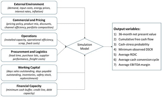
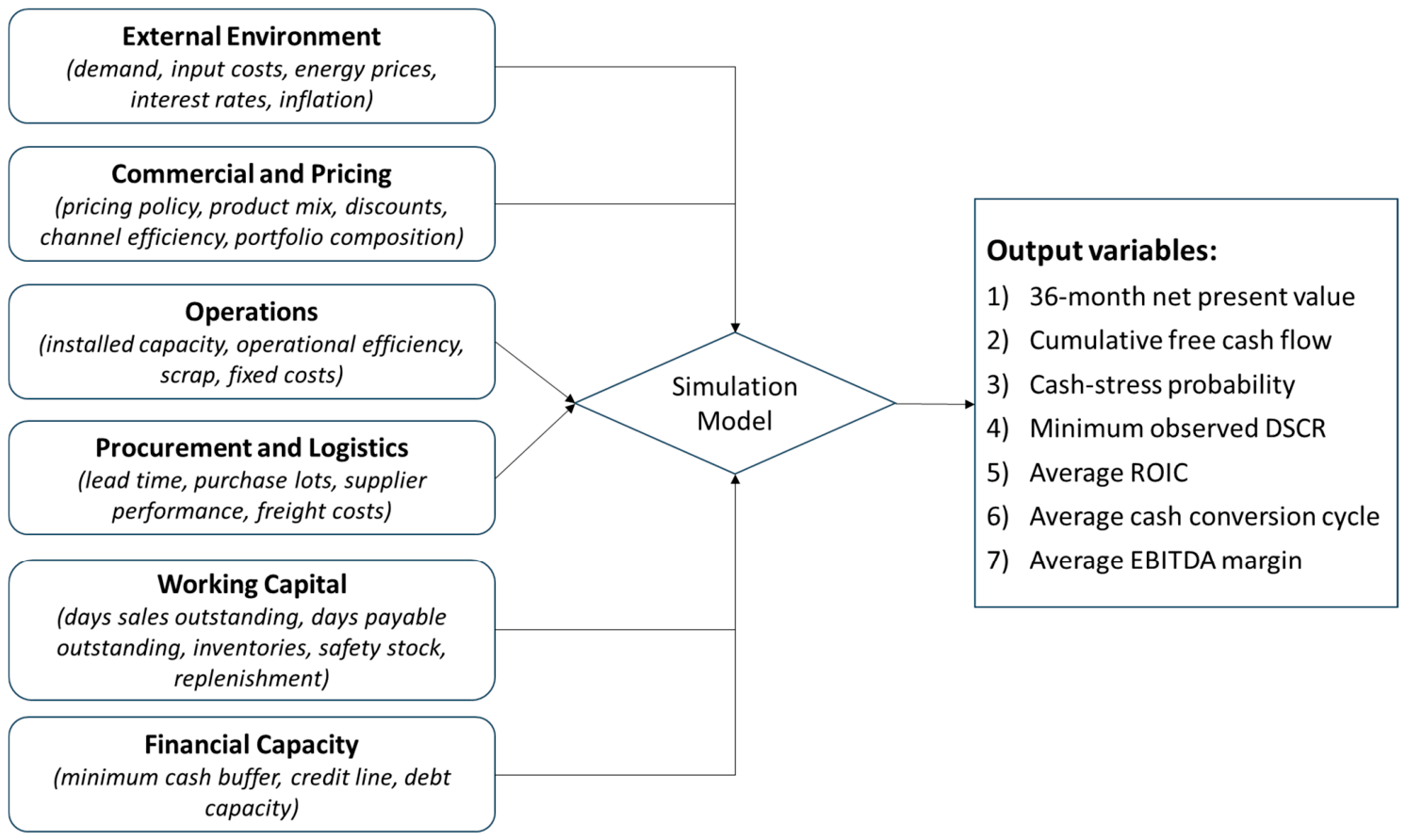

Disclaimer/Publisher’s Note: The statements, opinions and data contained in all publications are solely those of the individual author(s) and contributor(s) and not of MDPI and/or the editor(s). MDPI and/or the editor(s) disclaim responsibility for any injury to people or property resulting from any ideas, methods, instructions or products referred to in the content. |
© 2026 by the authors. Licensee MDPI, Basel, Switzerland. This article is an open access article distributed under the terms and conditions of the Creative Commons Attribution (CC BY) license.