


Abstract
The concentration of market capitalisation inside the S&P 500 rose sharply between 2016 and 2025, and it rose far faster than wealth concentration among American households. We establish this by treating index constituents as a population whose income is market capitalisation and applying the measurement apparatus of the income-distribution literature to annual cross-sections. Two construction choices do most of the work and are the paper’s first contribution: year-end membership is reconstructed from a dated historical constituent file rather than projected backwards from the current index, and prices and share counts are reconciled onto a common split basis. The two corrections do not work in the same direction. A roster projected backwards from today’s index produces a rising concentration trend whether or not concentration rose, while the split reconciliation raises the measured 2016 concentration rather than lowering it. A corrections waterfall quantifies each. Across 4443 firm–years, the share of index market capitalisation held by the five largest constituents rose from 13.4% to 30.0%, the Gini coefficient from 0.586 to 0.719, and the effective number of independent positions implied by the Herfindahl–Hirschman index fell from 112 to 43. The top-share trends survive imputation of every missing delisted firm at three plausible sizes, a balanced panel, and every specification of the inference we tried, including a bootstrap that resamples constituent firms rather than years at throughout. The Gini trend is significant under every imputation at , although, under the most adverse, its slope falls from 0.0133 to 0.0073 per year. The plug-in Gini understates inequality in fat-tailed samples, and the size of that correction depends on the distribution that is assumed to generate the data: it steepens the trend under a Pareto model, leaves it unchanged under a lognormal, and leaves it insignificant under a Pareto fitted at the Clauset–Shalizi–Newman exponent, so no corrected slope is quoted as the paper’s estimate. Over the same decade the top 1% share of US household net worth moved 0.65 percentage points, so firm concentration moved 24 to 30 times as far depending on the fixed-count basis used. An additive decomposition attributes 32% of the decade’s rise in the Theil index and 46% of the rise in the mean log deviation to the widening gap between digital and non-digital firms; the rest is dispersion within the two groups, so the movement is disproportionately but not wholly digital. Pareto tail indices are reported throughout as a diagnostic of tail shape rather than a headline result because the Hill and Clauset–Shalizi–Newman estimators of the same parameter disagree, a bootstrap goodness-of-fit test rejects the power law at the 5% level in seven of ten years, and the fitted trend does not survive a bootstrap that resamples firms rather than years. The second contribution is that negative finding, which bears on any study estimating tail indices from cross-sections of a few hundred firms.
1. Introduction
In 2016 the five largest constituents of the S&P 500 held 13.4% of the index’s market capitalisation. By 2025 the same five positions held 30.0%. Over that decade the top 1% of US households moved from 30.7% to 31.4% of the national net worth, a change of 0.65 points on the unrounded series. Corporate value concentrated roughly twenty-six times as fast as household wealth, and the effective number of equally weighted positions in the index, the reciprocal of its Herfindahl–Hirschman index, fell from 112 to 43. That reciprocal is a function of the index weights alone. It says nothing about the variances of the constituents or the correlations among them, so it measures how concentrated the weights became and not how much diversification was lost. Section 5.8 separates the two.
The distribution of firm size has been an object of study since Gibrat (1931), and the modern literature treats its upper tail as the signature of the growth process that generated it. What that literature rarely does is ask whether the distribution is moving, year by year, inside a fixed and economically meaningful population and how fast it moves relative to the distribution of household wealth that occupies so much more of the public argument. The question has become more pressing as a small number of technology firms have come to account for an unprecedented share of US equity market value, with consequences for portfolio risk that are immediate and measurable.
Three bodies of work bear on this. The first, from Gibrat (1931) through Axtell (2001), Gabaix (2009) and Luttmer (2007), characterises the firm size distribution as heavy-tailed and supplies the growth-and-selection mechanisms that generate such tails. It has not settled what the tail is: the debate between a Pareto or Zipf upper tail and a lognormal or mixed alternative is open, with Axtell (2001) finding an exponent that is indistinguishable from unity across the US firm census, Kondo et al. (2023) rejecting the Zipf value on establishment microdata, and Clauset et al. (2009) warning that samples of realistic size rarely discriminate between the candidates at all. That unsettled question is the starting point for this paper, and Section 5.5 reports a result that bears on it. The literature’s empirical work is also overwhelmingly cross-sectional: a distribution is fitted at a point in time and its exponent reported. The second, running from Rosen (1981) and Frank and Cook (1995) to D. Autor et al. (2020) and Grullon et al. (2019), documents rising concentration and superstar dynamics but measures them with product-market shares or aggregate markups rather than the distributional apparatus of the first body. The third, the income and wealth distribution literature of Piketty (2014), Saez and Zucman (2016) and Vermeulen (2018), has the measurement apparatus fully developed in Gini coefficients, top shares, decomposable entropy indices and tail indices with their inferential machinery but applies it to people.
No study we are aware of applies the third body of literature’s apparatus to the first’s object on an annual basis, which is what is required to ask how fast firm-size inequality moves and how that rate compares with the household benchmark. Doing so is not a matter of relabelling. It requires a panel in which membership is historical rather than projected, price and share bases are reconciled, and one company contributes one observation. It also requires inference that survives having ten annual observations rather than the hundreds a cross-sectional fit enjoys. Each of those requirements is a place where the measurement can fail silently, and the failures run in the direction of the finding.
The paper asks: to what extent did the distribution of market capitalization across S&P 500 constituents become more concentrated between 2016 and 2025, how does the rate of that change compare with the contemporaneous change in US household wealth concentration, and is the movement a market-wide shift in the firm size distribution or one concentrated in the digital sector? Four objectives follow. Construct an annual panel whose known failure modes are corrected and whose corrections are quantified. Measure concentration with estimators that do not require a distributional assumption, and establish which findings survive the survivorship, small-sample, and estimator-bias objections that ten annual observations invite. Decompose the change additively between the digital and non-digital groups rather than asserting a sectoral attribution. And report the portfolio-risk consequences, which follow directly from the same panel.
We treat index constituents as a population whose income is market capitalisation. Year-end membership for 2016–2025 comes from a dated historical constituent file; market capitalisations are built from year-end prices and share counts reconciled onto a common split basis; share classes are collapsed so that each company enters once. Concentration is measured by the Gini coefficient, fixed-count and proportional top shares, the Herfindahl–Hirschman index and its reciprocal, and the Theil index and mean log deviation, which decompose additively by group. Pareto tail indices are estimated by the Hill method and the Clauset et al. (2009) procedure. Trends are tested with Newey–West standard errors carrying the degrees-of-freedom correction and refer to ; the tail-index trend, whose significance turns out to depend on that choice, is additionally checked against a wild bootstrap and an exact permutation test on the year index.
Three contributions follow in the order that the evidence supports them.
First, and most securely, concentration rose on every measure that does not require a distributional assumption, and the rise is robust. The five-firm share went from 13.4% to 30.0%, the Gini from 0.586 to 0.719, and the effective number of positions from 112 to 43, each at on every specification of the inference we report. The top-share trends survive imputing every missing delisted firm at three plausible sizes and restricting to a balanced panel at in every case, with the slope steeper if anything under the most adverse imputation. The Gini trend is the more exposed of the two: under imputation at the sample minimum its slope falls from 0.0133 to 0.0073 per year and its p-value to 0.0016. Correcting the plug-in Gini for the fat-tailed small-sample bias of Fontanari et al. (2018) requires a model of the whole cross-section, and the correction is not sign-stable across the models that this paper entertains, so it is reported in tables in Section 5.3 and no corrected slope is carried into the claims. Against this, the top 1% share of US household net worth moved 0.65 percentage points.
Second, the movement is disproportionately but not wholly digital, and we report that as a decomposition rather than an assertion. The Shorrocks (1980, 1984) decomposition attributes 32% of the decade’s rise in the Theil index and 46% of the rise in the mean log deviation to the widening gap between the digital and non-digital groups; the remainder is dispersion within them. The digital group’s share of the value held in the estimated tail rose from 43% to 69%.
Third, and this is a negative result that we think is transportable, the Pareto tail index is not a reliable instrument at these sample sizes and we no longer rest any claim on it. Two standard estimators of the same parameter, computed on the same cross-sections, correlate at 0.39 and yield a marginal decline and no decline, respectively. A bootstrap goodness-of-fit test rejects the power law at the 5% level in seven of ten years and at the 10% level in eight. The fitted trend’s p-value moves from 0.025 to 0.255 across defensible choices of inference, and dropping a single year removes a third of the slope. A bootstrap that resamples constituent firms rather than years, which is the resampling unit the repeated appearance of the same companies in every annual tail calls for, widens the interval on every one of these trends to include zero. We report all of this and the accompanying corrections waterfall showing what each panel-construction decision is worth because the same traps await anyone repeating the exercise on another index.
Section 2 reviews the literature in terms of firm size distributions and their theoretical foundations, digital economics, superstar markets, and market concentration. Section 3 describes the data and the corrections. Section 4 sets out the estimators and the inference. Section 5 reports the findings, Section 6 discusses what they do and do not establish, Section 7 sets out the extensions that the design invites, and Section 8 concludes.
2. Literature Review
2.1. The Economics of Digital Goods
Shapiro and Varian (1998) set out the two properties that drive everything that follows. Digital information is non-rival, so one person’s use does not diminish another’s, and its marginal cost of reproduction is close to zero. Information is costly to produce and cheap to reproduce. A firm whose product is bits faces a cost structure in which the first unit carries the entire burden and every subsequent unit is nearly free.
Brynjolfsson and McAfee (2014) build on this to argue that digital progress has three characteristics: it is exponential, digital, and combinatorial. The exponential component is Moore (1965/1998), whose observation about transistor density has held for half a century and extends well beyond semiconductors to storage, bandwidth and sensing. The combinatorial component draws on Weitzman (1998), who models growth as the recombination of existing ideas, so the stock of possible innovations expands faster than the stock of components. Arthur (2009) makes the same argument from the history of technology, and Romer (1990) supplies the formal treatment of ideas as non-rival inputs that generate increasing returns.
Digital technologies are general purpose technologies in the sense of Bresnahan and Trajtenberg (1995): they diffuse across sectors, improve continuously, and require complementary innovation before their productivity effects appear. That last requirement explains the productivity paradox that Brynjolfsson (1993) identified. The underlying accounting problem is older: Solow (1957) found that capital deepening explained only about an eighth of the growth in US output per man-hour between 1909 and 1949, leaving the remainder to technical change and setting the terms for the debate that followed. Brynjolfsson et al. (2021) formalise the resolution as a J-curve in which intangible complements are accumulated before measured output responds. The mechanism matters here because it predicts that returns accrue to firms that have already built the organisational and intangible capital that digital technologies require, which is a concentrating force rather than a diffusing one.
Whether the resulting gains are large is contested. Brynjolfsson et al. (2003) estimate substantial consumer surplus from increased product variety online, and Jensen (2007) documents sharp welfare gains from information technology in a market with no prior price transparency. Against this, Cowen (2011) and Gordon (2016) argue that recent innovation has been narrower in its effects than the innovations of the late nineteenth and early twentieth centuries, and Bloom et al. (2020) show that research productivity has fallen sharply across many fields. We take no position on the aggregate growth question. What matters for this paper is distributional: whether the gains, however large, are concentrating.
2.2. Superstar Markets and Winner-Take-All Competition
Rosen (1981) explains why small differences in talent produce enormous differences in reward. When a seller’s output can be reproduced at low cost and consumers prefer the best available option, the best seller captures a share of the market out of all proportion to their margin of superiority. Rosen’s original examples were performers and surgeons. Digital goods generalise the structure because reproduction cost falls towards zero for any product that can be encoded as bits.
Frank and Cook (1995) extend the argument to competition in which rewards depend on relative rather than absolute performance. Among the mechanisms they enumerate are decision leverage, under which the value of marginally better judgement grows with the consequences riding on it, and network economies. A sergeant’s mistake costs a platoon, a general’s an army. Brynjolfsson and McAfee (2014) sharpen the network channel for digital goods specifically: network effects create demand-side economies of scale so that a product becomes more valuable to each user as more users adopt it. Where low marginal cost gives supply-side scale economies and network effects give demand-side ones, the two together make a market difficult for a second entrant to contest.
The empirical counterpart is a literature on top incomes. Kaplan and Rauh (2013) show that the rise in top earnings is broad-based across industries rather than confined to finance. They attribute this to scale: technology and organisational change have increased the assets under the control of any one decision maker. Levy and Murnane (2004) drew the boundary between what computers and people do well, placing expert thinking and complex communication on the human side. Acemoglu and Autor (2011) formalise it as a task framework in which routine work is displaced and abstract work complemented, Jaimovich and Siu (2020) link the resulting polarisation to jobless recoveries, and D. H. Autor (2019) traces how the occupational structure has reorganised around the surviving categories. Technology is not the only candidate explanation: D. H. Autor et al. (2013) attribute a substantial share of the decline in US manufacturing employment to import competition from China. Frey and Osborne (2017) and Acemoglu and Restrepo (2020) extend the displacement question to automation and robotics directly. Schumpeter (1942) supplies the older frame: creative destruction creates value for customers while eliminating incumbents, so winner-take-all markets are unstable as well as concentrated.
Most of this literature measures inequality among people, whether workers or top earners. The corresponding question for firms has been studied under different headings, and the two lines of work rarely meet.
2.3. Heavy Tails in the Firm Size Distribution
Firm sizes have been known to be heavy-tailed since Gibrat (1931) proposed that proportional random growth generates a lognormal distribution. Simon (1955) showed that a growth process with entry generates a power law instead, and Ijiri and Simon (1977) developed the application to business firms. Zipf (1949) gave the special case in which the tail exponent equals one, the point at which the largest member is roughly twice the second largest and the distribution has no finite mean.
Axtell (2001) established the modern benchmark, showing that US firm sizes follow Zipf’s law with a tail exponent that is statistically indistinguishable from unity across the full census of firms. Luttmer (2007) derives the result from a model of selection and growth, and Sutton (1997) reviews what Gibrat’s law does and does not explain. Kondo et al. (2023) qualify the benchmark: using establishment and firm microdata they find tails that are heavy but reject the Zipf value, a reminder that the exponent is an estimate rather than a constant of nature. A parallel literature on heterogeneous firms, following Melitz (2003), derives size dispersion from productivity differences and selection into export markets rather than from random growth alone. Gabaix (2009) surveys power laws across economic quantities, and Gabaix (2011) and di Giovanni and Levchenko (2012) show that, when the firm size distribution is sufficiently heavy-tailed, idiosyncratic shocks to individual firms do not wash out in aggregate. The tail index is therefore not only a description of inequality but a parameter governing macroeconomic volatility.
Estimating it is where the difficulties lie. Hill (1975) gives the standard estimator, which conditions on the largest k observations and trades bias against variance through that choice. Clauset et al. (2009) formalise the surrounding procedure: estimate the cutoff above which a power law holds, fit by maximum likelihood, and compare against alternatives by the likelihood-ratio test of Vuong (1989) rather than goodness of fit alone. Their central warning is that a heavy tail is often indistinguishable from a lognormal at realistic sample sizes, a point that Newman (2005) and Cirillo (2013) both emphasise and one this paper’s results confirm. Gabaix and Ibragimov (2011) give a rank-based correction for the regression approach. Fernholz (2002) develops the parallel apparatus for market capitalisation specifically, showing that the distribution of capital across a stock market has a stable rank structure that is amenable to the same tools. Ordoñez and Batac (2025) revisit the testing problem directly, comparing the available procedures for deciding whether a Zipf or Pareto law holds and finding that conclusions depend materially on which is used, a caution this paper’s own results bear out. Huang et al. (2024) track a Pareto exponent through a crisis rather than estimating it once, which is the closest methodological analogue to the exercise here and the same design in a different application; they too find that the exponent moves. Danielsson et al. (2001) propose a data-driven bootstrap rule for the tail fraction, an alternative to the fixed proportion used below that we return to in Section 6.3.
Which Mechanisms Generate a Heavy Tail, and Why It Matters Here
The tail exponent is not a free parameter: it is the fingerprint of a growth process, and the competing accounts make different predictions about what would move it. Gibrat’s law of proportionate effect, under which growth rates are independent of size, yields a lognormal in its pure form and only acquires a power-law tail when it is modified. Simon (1955) modifies it with entry: a constant inflow of small firms converts proportionate growth into a Pareto tail whose exponent is governed by the entry rate, so a fall in entry thickens the tail mechanically. Luttmer (2007) modifies it with selection: firms draw productivities, exit when they fall below a threshold, and the stationary size distribution inherits a Zipf tail from the balance between growth and the exit barrier, with the exponent tied to the gap between the growth rate of incumbents and the rate at which entrants displace them. Melitz (2003) supplies the trade-theoretic version in which selection into export markets rather than random growth generates the dispersion. Zheng and Hu (2025) embed the same selection logic in a macroeconomic model and show the size distribution responding to policy through entry and exit margins, while Chakrabarti and Tomar (2024) identify an organisational channel: the heavy tail of firm size is carried substantially by multi-plant firms, so what looks like a property of the size distribution is partly a property of firm boundaries. Di Guilmi and Fujiwara (2025) locate the mechanism in production networks instead, showing that the topology of the supply network shapes the firm size distribution it sustains.
These accounts are not nested, and this paper cannot separate them. What they share is the implication that the exponent is informative about entry, exit and selection, which is precisely why a decade-long movement in it would be interesting and establishing whether such a movement can be measured reliably at the sample sizes available is a prerequisite to interpreting one. Section 5.4 reports that it cannot, at least here, and the paper’s claims are set accordingly.
2.4. Rising Concentration and the Intangible Explanation
A large recent literature documents that US industries have grown more concentrated. Grullon et al. (2019) find increases in the majority of industries since the late 1990s, accompanied by higher profit margins. De Loecker et al. (2020) estimate that average markups rose from 1.21 to 1.61 times marginal cost between 1980 and 2016, with the increase driven by the upper tail of the firm distribution rather than a general shift. Bajgar et al. (2019) confirm the pattern in Europe as well as North America. Mertens and Mottironi (2025) sharpen the link between size and market power, estimating markups and markdowns along the size distribution and finding that the market-power gradient rises with size, so reallocation towards the largest firms is not distributionally neutral; Dobbelaere and Wiersma (2025) trace the same reallocation to competitive shocks, which is the selection channel of Section 2.3 observed in the data. Whether concentration takes the same form under different legal and ownership regimes is an institutional question in the sense of Acemoglu and Robinson (2012) and one that this paper does not answer; we note in Section 7 why the cross-sectional evidence we were able to assemble is not adequate to answer it.
The exercise closest to this one is Metelski and Sobieraj (2024), who apply Gini coefficients to S&P 500 constituents and evaluate concentration-driven portfolios. The quantity they measure is trading volume rather than market capitalisation, and their question is whether concentration can be traded rather than whether it is rising. The overlap is nonetheless the clearest evidence that the apparatus transfers to index constituents, and their portfolio framing anticipates the risk quantities reported in Section 5.8.
D. Autor et al. (2020) supply the mechanism that connects concentration to distribution. Industries have become winner-take-most, and, because the largest firms have lower labour shares, reallocation towards them lowers the aggregate labour share without any firm changing its own behaviour. Karabarbounis and Neiman (2014) document that decline across countries and industries, and Barkai (2020) shows that the capital share fell alongside it, with the residual accruing to profit. Philippon (2019) and Eeckhout (2021) read the same evidence as a failure of competition policy.
The competing explanation is intangible capital. Corrado et al. (2009) showed that intangible investment had grown to rival tangible investment in the United States, and Haskel and Westlake (2017) argue that intangibles have properties, scalability, sunkenness, spillovers and synergies that systematically favour large incumbents. Crouzet and Eberly (2019) decompose rising concentration into intangible-intensity and market-power components and find both present. The distinction matters for interpretation: concentration produced by scalable intangible assets is a different phenomenon from concentration produced by barriers to entry, even where the measured tail index is the same. Our estimates cannot separate the two, and we are explicit about that limit.
2.5. Measuring Inequality Across Different Populations
The measures used here are standard in the study of income and wealth. Cowell (2011) gives the treatment of the Gini coefficient and top shares and their sensitivity to different parts of the distribution. Hirschman (1964) records the origin of the concentration index that bears his and Herfindahl’s names, now the standard instrument of competition authorities.
Applied to households, these measures have produced a well-established set of facts. Piketty and Saez (2003) reconstructed US top income shares from tax records, Saez and Zucman (2016) extended the exercise to wealth by capitalising income flows, and Piketty (2014) placed the results in a long-run framework in which the return to capital exceeding the growth rate drives wealth concentration. Alstadsæter et al. (2019) show that these estimates understate the top share once offshore evasion is accounted for. The Distributional Financial Accounts introduced by Batty et al. (2019) put the household wealth distribution on a quarterly basis that is consistent with the national accounts and supply the household series used in this paper.
The stakes of that distribution are not confined to the accounts. Olshansky et al. (2012) document falling life expectancy among non-Hispanic white Americans without a high school education, Lusardi et al. (2011) find that close to half of US households could not raise $2000 within a month, and DeBacker et al. (2013) show from tax records that the rise in US income inequality since the late 1980s came from the persistent component of income rather than the transitory one. Brynjolfsson and McAfee (2014) treat these as the spread that accompanies the bounty, which is the reason that the firm-side measurement in this paper is worth setting beside the household-side one.
The gap this paper addresses is that the same apparatus is rarely turned on firms. The concentration literature reviewed above measures shares of sales or employment within industries, typically as four-firm or eight-firm ratios, and the heavy-tail literature estimates a tail exponent on a single cross-section or a pooled sample. Neither produces an annual series of distributional statistics for a defined population of firms that can be set beside the household series. Bessembinder (2018) comes closest in spirit, showing that the entire net wealth creation of the US stock market since 1926 is attributable to about 4% of listed firms, but the calculation is cumulative rather than a year-by-year distribution.
Doing that requires solving a measurement problem that the household literature does not face. Household panels are constructed to be representative; index membership is not a panel at all but a changing roster, and the firms that leave it are systematically the smaller and less successful ones. Any study of index concentration over time must reconstruct membership rather than assume it, which is where Section 3 begins.
3. Data
3.1. Two Inputs, and Why Both Are Needed
The panel requires two things: who belonged to the index in a given year and what each member was worth at the end of it. Membership and market value come from separate sources, and conflating them is the single most common way this measurement goes wrong.
Taking today’s index and projecting it backwards produces a sample of firms that survived. Because survival correlates with size and size is the quantity under study, such a sample guarantees a finding of rising concentration whether or not concentration rose. That asymmetry belongs to the membership reconstruction alone. The split reconciliation of Section 3.3 does not share it. Tables in Section 5.3 show that removing it raises measured 2016 concentration. Share counts carried back across a later reverse split overstate the firms that shrank by more than they understate the firms that grew, and tables in Section 5.3 trace the effect to a single constituent. The two corrections therefore, address distinct biases, and we no longer describe them as one. Table 1 lists every source used. The rest of this section explains what each contributes and where it fails.
Table 1.
Data sources. All series are public. The historical constituent file and the market data are the two inputs from which the panel is built; the remaining sources support the household comparison and the cross-country section.
Table 2.
Reconciling the price and share bases. Yahoo Finance reports a split-adjusted close but an unadjusted share count, so the product understates every year preceding a split by the cumulative split factor. Column 3 gives the uncorrected product, column 4 the corrected one, and column 5 an independently reported market capitalisation. Microsoft, which has not split since 2003, is unaffected and serves as a control. Values in USD billions. Source: authors’ calculations.
3.2. Index Membership
Year-end membership comes from a published historical-constituents file covering 2 January 1996 to the present, distributed under an MIT licence and compiled from index change announcements. Each record is a date and the full list of tickers in the index on that date. The roster for year t is the last snapshot on or before 31 December of year t. Over 1996–2025 this yields 14,143 roster–years and 1104 distinct tickers against a mean roster of 471 firms.
We first attempted to reconstruct membership from the change log on the Wikipedia article List of S&P 500 companies, walking additions and removals backwards from the current constituent list. That approach fails, and the reason is worth recording. The table is titled Selected changes: it is curated rather than complete, and it does not extend to the 1990s. A reconstruction built on it is wrong in the early years in a way that leaves no trace in the output.
Two guards enforce the distinction. The pipeline refuses to build a panel without a membership file rather than falling back on the current ticker list. It then counts how many firms in each roster have since left the index and halts if that count is zero since a roster containing only present-day survivors is not a historical roster.
3.3. Prices, Share Counts, and the Split Basis
Prices and share counts come from Yahoo Finance through the yfinance library. Market capitalisation is the year-end closing price multiplied by shares outstanding. Both need a mapping rule because neither series is observed on 31 December. The price is the last daily Close on or before 31 December of year t with auto_adjust=False so that the series is adjusted for splits but not dividends, which is the basis Equation (1) below assumes. The share count is the last get_shares_full observation falling within calendar year t; that series is irregular, reported at filing dates rather than on a schedule, so where a year contains no observation the nearest available count is carried forward, and where a year precedes the first observation it is carried backward. Carrying backward is the weaker operation and one of the two reasons the estimation window starts in 2016, as Section 3.5 explains.
The two series are not reported on the same basis, and multiplying them directly is an error. Yahoo reports a closing price adjusted for all subsequent stock splits, expressed in today’s share units, while get_shares_full reports the share count outstanding on that date. For any firm that split after year t, the product understates market capitalisation by the cumulative split factor. Apple’s 2016 value comes out four times too low, Amazon’s twenty times, and Nvidia’s forty.
The correction puts the share count on the price’s basis. Writing for the reported share count of firm i at year-end t and for the product of every split ratio recorded after that date,
where is the ratio of the sth split of firm i and its effective date. The adjustment touches 3087 of 10,111 firm–years.
The convention matters and is easy to get backwards, so we state it explicitly and work one case through. Yahoo’s Close is expressed in today’s share units: a price series for a firm that later split four for one has every pre-split price divided by four so that the series is continuous. get_shares_full, by contrast, reports the share count as it stood on the observation date in that date’s units. The two are therefore on different bases whenever a split falls between the observation date and the present, and the product is too small by exactly the cumulative split factor. The correction multiplies the historical share count up to today’s units rather than unadjusting the price, which is equivalent and avoids re-deriving a price series.
Take Apple at the end of 2016. Yahoo reports a closing price of $28.95, which is the $115.82 Apple actually traded at divided by the 4:1 split of 31 August 2020. It reports 5.332 billion shares outstanding, which is the count as of 2016 and is not divided by anything. The naive product is . Apple was not a $154 billion company in 2016. There is one split after 2016, of ratio 4, so and Equation (1) gives against an independently reported $609 billion: a deviation of 1.4%, which is the residual from using a year-end close rather than the exact date the benchmark uses. NVIDIA in 2016 carried a 4:1 split in 2021 and a 10:1 split in 2024, so and an apparent $1 billion becomes $58 billion. Microsoft has not split since 2003, so and both columns agree; it is the control that shows the correction does nothing where nothing is required.
Table 2 validates the result against ten market capitalizations that can be checked independently. The largest deviation is 1.4%. The benchmark column is market-capitalization history from macrotrends.net, cross-checked against the share count on each firm’s 10-K cover page for the corresponding fiscal year.
Two limitations of this validation should be stated. The ten firm–years are all large surviving firms, which is the population in which Yahoo’s split history is most complete, so the exercise establishes that the correction is applied correctly rather than that Yahoo’s split records are exhaustive.
That is the weaker of the two statements, and the population it omits is the one that matters most. Firms that later left the index are where Yahoo’s split and share-count histories are least reliable, and they are absent from the validation for the same reason they are absent from the early cross-sections: the source retains no usable series for them, so no benchmark capitalisation can be assembled to check against. Extending the validation to a random sample stratified by size and later exit would require a second vendor with delisted coverage, which we do not have. The consequence is stated here rather than left implicit: Table 2 establishes that the reconciliation is correct on firms the source covers well, and the coverage exercise of Section 5.3, rather than this table, is what assesses the effect of the firms it covers badly.
And the pipeline reads a live API whose outputs are not stable across time: Yahoo restates share counts and the auto_adjust default in yfinance changed at version 0.2.51, which determines whether Close is adjusted for dividends as well as splits and therefore whether Equation (1) reconciles the intended two objects. We pin the library version at yfinance [version], record the retrieval date of [retrieval date], and deposit the built panel so that the numbers reported here are reproducible even though a fresh download would not reproduce them exactly; see the data-availability statement.
This matters beyond bookkeeping. Firms that split are disproportionately the fast-growing digital firms, so the uncorrected panel understates precisely the early-period values of the firms the paper is about and manufactures a concentration trend out of an accounting mismatch.
3.4. One Firm, One Observation
Dual-class firms appear once per listed class. Alphabet enters twice in the 2025 cross-section as GOOGL and GOOG, and Yahoo reports a market capitalisation of roughly $3.8 trillion against each of them, which is the company-wide figure and not the value of either class. Left alone this counts one company twice and places the duplicate near the top of the distribution, which is the only region the tail index is estimated from.
Share classes are collapsed by company name rather than ticker because the base symbols of a dual-class pair need not resemble each other: RCI-A and RCI-B share a stem but GOOG and GOOGL do not, and a symbol-matching rule silently misses Alphabet, which is the largest case in the sample. The rule for combining the classes requires care because Yahoo’s behaviour is not uniform. For some dual-class firms get_shares_full returns a class-specific count, in which case the classes’ capitalisations must be summed; for others it returns the same company-wide count against both tickers, in which case summing double-counts the firm. We distinguish the two empirically: if the share counts reported for the classes agree to within a tolerance, the count is company-wide and the class capitalisations are averaged; if they differ materially, they are class-specific and are summed. The largest class is retained as the identifier and the treatment applied to each multi-class firm in each year is recorded in the deposited output, so the choice is auditable rather than asserted.
That tolerance was set at one percent in the build used for the submitted version, and it was too tight. In the 2016 cross-section, and in that year alone, Yahoo reports company-wide counts for Alphabet’s two classes that differ by 2.67 percent, so the rule classified them as class-specific and summed them. Alphabet then entered 2016 at $1080 billion, 5.82 percent of index value and ahead of Apple against an actual capitalization of about $539 billion. Every other multi-class firm–year in the window was treated correctly. The tables in this version are computed on the deposited panel in which multi-class counts are treated as company-wide throughout, and Alphabet enters 2016 at $540 billion.
The operation conserves the index total. In 2025 it merges three multi-class companies, reducing 491 listings to 488 firms.
3.5. Coverage and the Estimation Window
Yahoo does not retain price history for most delisted tickers. Of the 1128 tickers requested, 734 return a usable series and 394 return nothing. Every one of the 394 is a firm that has left the index; no current constituent is missing. This is a property of the source rather than the request, and it binds hard: a licensed panel such as CRSP or Compustat carries delisted returns and would remove it.
The consequence is visible in Figure 1. Coverage rises monotonically from 40% of the 1996 roster to 97% of the 2025 roster because, the further back one looks, the larger the share of that year’s index that has since been acquired or wound up.
Figure 1.
Shareof each year’s reconstructed roster with usable market capitalization data. The gradient is the survivorship constraint made visible: delisted firms lose their price history, and the early rosters are mostly firms that have since delisted. The shaded band is the estimation sample. Source: authors’ calculations.
Within the estimation window this gradient runs from 80.8% of the 2016 roster to 97.0% of the 2025 roster, and it is a survivorship problem in its own right, not merely a description of the source. Each annual cross-section is the true roster minus a set of systematically smaller firms, and that set shrinks sixfold over exactly the decade across which the trends are fitted, so the 2016 and 2025 statistics are computed on objects that differ in a way that co-moves with the finding. Reconstructing membership removes the backward-projection bias but not this one. Section 5.3 assesses it by imputing every missing firm–year at three plausible sizes and re-estimating on a balanced panel and reports what each exercise leaves standing. The short answer is that the concentration results survive all four scenarios and the tail-index trend does not, which is one of the reasons for the priority the revised paper gives them.
The estimation sample is the longest unbroken run of years clearing an 80% coverage floor, which gives 2016–2025. Requiring the run to be contiguous is deliberate. Taking every year that clears the floor admits isolated early years whose samples are not comparable to the modern ones, and splicing them into a trend inverts its sign.
The 80% figure is a convention and one that the results do not depend on. Results in Section 5.6 re-estimate at floors from 0.70 to 0.90: every floor from 0.70 to 0.80 selects the same contiguous run and therefore returns an identical slope and p-value because coverage jumps from 62% in 2015 to 82% in 2016 and there is no year in between for a floor to discriminate on. Only at 0.85 does the window shorten, to seven years, and at 0.90 it becomes too short to fit. The threshold is insensitive across its whole defensible range, which is what the choice requires in place of a justification from first principles.
A second and unrelated constraint points at the same start date. Yahoo’s share-count history begins in 2015: before that year no share count is observed and every value must be carried backwards from a later date, so pre-2016 market capitalisations combine a period price with a modern share count. Two independent limitations agreeing on the same window is a reason for confidence in it, not an apology for it.
The resulting panel holds 4443 firm–years and 554 distinct firms across ten years.
3.6. Plausibility Screen
Two firm–years in the built panel fail an absolute plausibility check. Paramount Global enters at a price of $101,200 in 2022 and $18,800 in 2023 against an actual price near $17: an error of three orders of magnitude. Combined with the firm’s reported share count, the 2022 figure implies a market capitalisation of $66 trillion, which would make one firm two thirds of the index and dominate every statistic computed from that cross-section.
The screen is deliberately narrow: a price ceiling of $10,000 per share, which no US common share except Berkshire Hathaway A approaches, and a second rule described below. Removing a firm flagged in any year from the window entirely would be too blunt, and Paramount is the only firm the screen flags. Paramount is a communication services firm and therefore in the digital group, whose tail is ten firms, so deleting it from all ten years is not a neutral act. The revised screen removes the offending firm–years rather than the firm. Re-fetching Paramount directly establishes that the corruption is in the source and not in our pipeline since Yahoo returns a price of $101,200 for 2022 and $18,800 for 2023 against an actual price near $17, and the price ceiling flags 2021 on the same grounds. The screen described below compares the flagged price against a reference closing price for the same date, taken from the firm’s own filings and the published historical quotations of the listing exchange. Those sources establish that the Yahoo figures are wrong, which is what the screen requires, but they do not supply the split-adjusted close paired with the matching share count that Equation (1) needs, and assembling that for three firm–years by hand would introduce a basis that is inconsistent with the other 4450. The three flagged firm–years are therefore excluded rather than repaired, and 2024 and 2025 are restored.
Tables in Section 5.6 report the full-sample estimates with and without the firm, including a 2021 row showing what restoring that year would do if its price were trustworthy. The largest effect on any annual tail index is 0.008 and on any Gini 0.0005, so the deletion was not driving the aggregate result, but the exercise belonged in the paper and was not there.
The second rule in the submitted screen was a ceiling of 15% on any single firm’s share of its index–year. That rule is defined on the quantity the paper is measuring, and a study arguing that concentration is rising should not carry a filter that begins deleting real observations if the argument continues to hold. It does not bind anywhere in the present sample since the largest single-firm share observed is well below it, but we have replaced it with an external test that does not reference the outcome: a firm–year is flagged if its implied market capitalisation disagrees by more than an order of magnitude with the value implied by the firm’s own reported share count and an independent closing price for the same date. On this sample the two rules flag the same two firm–years.
An earlier version of the screen also flagged prices far from a firm’s own median, which removed Nvidia, whose split-adjusted price moved by a factor of thirteen. A rule that deletes Nvidia from a study of technology concentration is worse than the problem it solves, and the relative test was dropped.
3.7. Household Benchmark
The household comparison uses the Federal Reserve’s Distributional Financial Accounts, series WFRBST01134, the share of total US household net worth held by the top 1% of households averaged to annual frequency.
4. Concepts and Methodology
4.1. Firms as a Population
We treat the constituents of a stock index as a population of individuals whose income is market capitalisation. Everything the inequality literature does to household income then applies without modification: Gini coefficients, top shares, and, above all, the Pareto tail index.
The move is not merely a metaphor. Firm size has been known to follow a heavy-tailed distribution since Gibrat (1931), and Axtell (2001) showed that US firm sizes follow Zipf’s law with a tail exponent that is indistinguishable from unity. What has not been done is to apply the machinery of income-distribution measurement to index constituents year by year and ask whether the resulting inequality is rising and where.
That question is testable, and Brynjolfsson and McAfee (2014) state it in a form that makes four specific predictions.
4.2. Four Claims
The Second Machine Age argues that digital goods are non-rival, cost almost nothing to reproduce, and are subject to network effects, so digital markets tend towards winner-take-all outcomes. The argument extends Rosen (1981) on superstar markets and Frank and Cook (1995) on winner-take-all competition. Four claims follow, and each maps onto a statistic the data can produce.
- C1
- Superstar markets follow a power law in the upper tail. Testable in absolute terms by the Clauset–Shalizi–Newman bootstrap goodness-of-fit statistic for the fitted power law itself, which asks whether a power law is an acceptable description of the tail, not merely whether it beats a rival.
- C2
- The economy is a mixture: lognormal through the body of the distribution, power law at the top. This is not testable by the power-law-versus-lognormal comparison above the cutoff. Both C1 and C2 imply a power-law tail above some threshold, so a comparison run only above the threshold cannot separate them, and an inability to discriminate is evidence for neither. The separable version fits a lognormal to the full cross-section, body included, and asks whether the upper tail requires a Pareto extension beyond what the fitted lognormal predicts. We report that test in Section 5.5 and record that the submitted version’s reading of the non-separation result as “the result C2 predicts” inverted the logic.
- C3
- Digitisation brings non-rivalry and network effects, so digital markets should show fatter tails than the rest. Testable by estimating the tail index separately for digital and non-digital firms.
- C4
- The bounty from digital technology accrues to a narrowing group, so concentration should have risen. Testable as a trend in the tail index and concentration measures.
C1 and C2 concern distributional shape. C3 and C4 concern direction, and both predict a falling tail index since a smaller index means a fatter tail.
4.3. Concentration Measures
Notation is fixed here and used throughout. In a given year the cross-section contains n firms, and is the market capitalisation of firm i for in no particular order. Writing the same n values in ascending order gives the order statistics
so that is the largest firm and the kth largest. The two are the same numbers: indexes firms; indexes positions in the sorted sequence. Statistics that depend on rank are written in , and statistics invariant to ordering are written in . Note that , so the denominators below may be read either way.
We report three standard measures. The Gini coefficient,
summarises dispersion across the whole distribution and requires the ascending ordering since each value is weighted by its rank i. The top q share,
sums the largest values, which sit at the top of the ordering, and is reported at .
The ceiling in Equation (4) is not innocuous over a decade in which n grows. With in 2016, ; from 2017 onward and . The top 1% column therefore compares a four-firm share in 2016 against a five-firm share thereafter, and on 2016 values the fifth-largest constituent is worth about two percentage points of the index, so part of the headline change is a ceiling-function artefact rather than a movement in the distribution. We therefore report fixed-count shares, the share held by the largest 5, 10 and 25 firms, alongside the proportional shares throughout and compute the headline change and the firm-versus-household ratio on the fixed-count basis. Results in Section 4.6 state how many firms enter the top 1% column in each year. The substantive conclusion is unchanged; the magnitude is 16.7 rather than 18.7 percentage points, and quoting the larger figure without noting the change of base would have been an overstatement.
The Herfindahl–Hirschman index,
weights the largest firms most heavily. It is a sum over all firms of squared shares, so it does not depend on the ordering and is written in the unordered .
H is not introduced here as the measure competition authorities use because that framing does not transfer. S&P 500 constituents do not compete with one another in a product market, so an antitrust reading of an index-level H has no referent; and in the units those authorities use, the values reported below are 89 points in 2016 and 234 in 2025, never exceeding 235 against a threshold of 1500, below which the US merger guidelines treat a market as unconcentrated, so the antitrust scale would make this paper’s finding look like no finding at all. What H does measure here, and measures well, is portfolio concentration. We therefore report its reciprocal,
the effective number of independent equally weighted positions the index is equivalent to. Within-industry concentration, which is the quantity the competition question actually requires, is measured directly by Grullon et al. (2019) and is not what an index-level H estimates.
Two further measures are added in this revision because the group attribution requires them. The Theil index and the mean log deviation,
belong to the generalised entropy family and decompose additively and exactly into within-group and between-group components (Shorrocks, 1980, 1984). Writing g for groups with population shares and income shares ,
This is the tool the paper’s framing implies. There is no additive relationship between an aggregate Hill index and two group Hill indices since they are three separate fits to three different tails at three different values of k, so showing that one group’s index falls and the other’s does not is consistent with the aggregate movement being digital but is not a decomposition of it. Equation (8) produces three numbers that sum to the total, and Section 5.6 reports the answer they give.
None of these requires a distributional assumption, which is why they carry the argument where the tail index cannot.
4.4. The Pareto Tail Index
A variable follows a Pareto tail if, above some threshold ,
The exponent is the object of interest. A smaller means a heavier tail and more of the total held by the largest members. At the distribution is Zipf, the case Axtell (2001) finds for US firms and Gabaix (2009) surveys across economic quantities.
We estimate with the Hill estimator (Hill, 1975), written here in the same ascending order statistics of Equation (2). Using the k largest observations, , each measured against the threshold immediately below them,
The estimator trades bias against variance through k: a small k uses only the extreme tail and is noisy; a large k reaches into the body and is biased. We set for the full cross-section, which gives tails of 39 to 48 firms, and report the Hill plot of against k so the reader can judge the stability of that choice directly.
The fixed proportion is a convention, not a derivation. Danielsson et al. (2001) give a double-bootstrap rule for selecting the fraction from the data, and the Clauset–Shalizi–Newman procedure of Section 4.5 selects a threshold by a different criterion again. Section 5.4 reports what happens when the paper’s two estimators are put side by side. They do not agree, and the apparent decade-long decline in the tail index is present under one and absent under the other. We therefore report throughout as a diagnostic of tail shape and rest no claim on its trend. The distribution-free concentration measures of Section 4.3 carry the paper.
Where an interval for is needed we use the exact small-sample distribution rather than the normal approximation. For a Pareto tail, ∼, so an exact interval is . At the that binds for the digital group this distribution is markedly right-skewed, so symmetric normal bands would be the wrong shape as well as the wrong width and are not used.
4.5. Which Distribution Fits
Claims C1 and C2 are about model choice, not a parameter, so we test them with the procedure of Clauset et al. (2009). The cutoff is chosen to minimise the Kolmogorov–Smirnov distance between the empirical and fitted distributions above the cutoff, is estimated by maximum likelihood on the resulting tail, and the fitted power law is compared against lognormal and exponential alternatives by the normalised likelihood-ratio test of Vuong (1989). A positive ratio favours the power law and a p-value below 0.05 makes the sign meaningful.
One convention needs stating because getting it wrong shifts every estimate by exactly one. The powerlaw implementation reports the exponent of the density, , whereas the Hill estimator targets the exponent of the survival function in Equation (9). The two differ by unity: . We report both on the survival convention. The estimators are verified against draws with known of 1.0, 1.5 and 2.5 before use.
4.6. Digital and Non-Digital
C3 requires a partition. A firm is classified as digital if its GICS sector is information technology or communication services or it is one of nine platform firms that GICS places elsewhere but whose economics are those of a digital market: Amazon, Tesla, Netflix, Booking, eBay, Airbnb, Uber, DoorDash and Shopify.
The classification is coarse, and deliberately so. It is fixed in advance, applies uniformly across years, and does not depend on the outcome. A finer partition estimated from the data would risk selecting on the variable being explained.
The nine hand-added firms are a judgment, so Table 3 reports the group contrast with them removed and the two largest of them, Amazon and Tesla, removed singly and together. The magnitude of the between-group share depends on those two. Amazon carries 6.1 percentage points of the Theil share and Tesla 4.6, roughly a third of the headline figure between them. On GICS sectors alone the between-group component falls from 31.9% to 22.5% of the rise in the Theil index and from 46.1% to 31.8% of the rise in the mean log deviation. The sign and the significance do not move. Under every variant the between-group component carries a substantial minority of the rise, and the trend in the tail-index gap is significant at . We read the reported partition as the one that best matches the economic claim and the pure-GICS partition as the conservative floor. The paper’s statement that the movement is disproportionately but not wholly digital holds on both.
Table 3.
The group contrast under alternatives to the reported classification. The first row is the partition of Section 4.6. The second removes the nine platform firms added by hand and keeps the GICS sectors alone, and the last three remove the two largest of the nine, singly and together. On the reported partition the between-group component carries 31.9% of the rise in the Theil index and 46.1% of the rise in the mean log deviation. Amazon is worth 6.1 percentage points of the Theil share and Tesla 4.6, so the magnitude depends on them. The sign and the significance do not. On GICS alone the between-group component still carries 22.5% of the Theil rise and 31.8% of the mean log deviation, and the trend in the tail-index gap is significant under every variant. Source: authors’ calculations.
Two features of the group estimate need care. The digital group holds 49 to 91 firms, so would give a tail of five. We floor the tail at . This does not make the two groups comparable at tail sizes of the same order, and the floor is not occasional. It binds in every year: never reaches 10 for the digital group, so throughout, while the non-digital group at to 382 uses to 38. Worse, the digital group’s tail fraction therefore falls monotonically from 0.19 in 2017 to 0.11 in 2025, a near-halving across exactly the window over which its tail index falls. Since the Hill estimator’s bias depends on how far k reaches into the body relative to n, the submitted specification had a design parameter drifting in lockstep with the effect it was measuring. Section 5.6 re-estimates the group series holding fixed and equal across groups and at several fixed values of k and reports what survives.
Sector labels come from the current constituent table, so firms that left the index before that table was written carry no label. Those 414 firm–years, 9.3% of the window, are excluded from the group contrast while remaining in the aggregate. The excluded firms are departures by construction, hence smaller and less successful, and they are concentrated in the early years for the same reason as the coverage gradient. Their absence compresses the measured dispersion of whichever group would have held them, which tilts the comparison towards the finding rather than against it; Section 5.3 reports the magnitude of the equivalent effect on the aggregate, and the group contrast should be read as carrying at least as much of it.
4.7. Trends
Each annual statistic is regressed on a centred year index,
with standard errors computed by the heteroskedasticity- and autocorrelation-consistent estimator of Newey and West (1987) at three lags for the aggregate series and two for the group series. Annual concentration measures are persistent, and treating their errors as independent would overstate precision.
Three features of the inference need stating.
First, the standard errors carry the degrees-of-freedom correction, and the resulting statistic refers to rather than a standard normal. Computed without the correction and against a normal reference, the resulting p-values are more permissive of the two choices on both counts. Tables in Section 5.4 report the full grid so the sensitivity is visible rather than asserted.
Second, with and a Bartlett kernel at a bandwidth of 30% of the sample, HAC asymptotics do not apply in the form usually invoked. This is the regime Kiefer and Vogelsang (2005) characterise, and they show the Bartlett kernel to be the most size-distorted of the common choices. Their own remedy is fixed-b asymptotics, under which the limiting distribution depends on the bandwidth ratio and the critical values are non-standard; we do not apply it and cite the paper for the diagnosis rather than the cure. We therefore report results across lag truncations of 0 to 3 and supplement the parametric tests with two procedures that do not rely on the asymptotics at all: a wild bootstrap with 20,000 replications and an exact permutation test on the year index, which, at , is cheap, although it requires the annual observations to be exchangeable under the null and so is not assumption-free. Where the three disagree, we report the disagreement rather than the most favourable of them.
Third, Equation (11) treats each annual statistic as measured without error, which is defensible for the Gini and the top shares and is not defensible for , whose standard error is printed in the same table and runs from 0.165 to 0.246 for the aggregate and 0.200 to 0.572 for the digital group. For the tail-index series we therefore also report a weighted least squares fit with weights and a firm-level bootstrap that resamples constituents within each year, re-estimates , and refits the trend, which handles the estimation error and the cross-sectional dependence together. Endpoint comparisons are reported with their standard errors rather than as bare numbers.
C3 is tested by regressing the annual gap on the year index. The submitted version also reported a paired t-test on the same nine differences and presented the two as answering different questions. They do not. The paired test is computed on the same nine numbers, which have a lag-one autocorrelation of 0.70 and a clear trend, so the independence assumption behind the t-statistic fails and its is not interpretable. Two tests on one series, one of them invalid, are not mutual corroboration. The paired test is withdrawn as evidence and replaced by a permutation test on the year labels; Results in Section 5.6 shows all three, so the withdrawal is auditable.
4.8. What the Design Guards Against
Four decisions exist to prevent an artefact from being read as a result, and each is stated here so that the results can be judged against them.
Membership is reconstructed rather than projected backwards, so historical cross-sections contain firms that have since delisted. The price and share bases are reconciled through Equation (1), so no firm–year is scaled by a stray split factor. Share classes are collapsed, so no company appears twice at the top of the tail. And the estimation window is a contiguous run rather than a set of qualifying years, so no trend is fitted across a gap in which nothing was measured.
Every one of the four was added after an earlier version of the analysis produced a result that the correction removed or reversed. We state plainly what that sentence implies: the specification was arrived at in the course of the analysis after seeing outcomes rather than pre-specified. We think the corrections are right on their merits and would defend each independently of what it does to the result, but the reader is entitled to know the order.
Tables in Section 5.3 report the headline statistics and the fitted trend under four builds: today’s roster projected backward, then the reconstructed membership without the split reconciliation, then without the dual-class collapse, and then the full specification. Reading down the slope column shows that the naive backward-projected roster produces a steeper and more significant tail-index trend than the corrected panel, so the corrections work against the headline rather than towards it. That is the most transportable result in the paper for anyone repeating the exercise on another index, and it had no table behind it. The table itself is reported with the other robustness exercises as Table 11 in Section 5.3.
5. Results
5.1. The Sample
The estimation panel covers 2016–2025: 4443 firm–years, 554 distinct firms, and between 391 and 488 constituents per year. The total market capitalisation of the sample rises from $18.0 trillion in 2016 to $61.3 trillion in 2025.
The panel reported here was rebuilt from the raw sources for this revision. The dual-class rule of Section 3.4 and the plausibility screen of Section 3.6 were stated and applied explicitly. Because Yahoo restates share counts over time, a panel rebuilt at a later date does not reproduce an earlier build exactly; a year-by-year reconciliation between the deposited panel and the build it replaces is included in the deposited output.
Table 4 reports the annual cross-sections.
Table 4.
Concentration and tail index of S&P 500 market capitalisation, 2016–2025. N is the number of constituents with usable market-cap data; total is the summed market capitalisation of that sample. is the effective number of independent positions implied by the Herfindahl–Hirschman index. The top 1% column is the top share of Equation (4), and the adjacent column reports how many firms that is (four in 2016 and five thereafter), so the column is not comparable across the two dates. The top 5 and top 10 columns are fixed-count shares and are comparable; they are the basis on which the paper’s headline figures are quoted. The Hill estimate uses the largest firms and is reported here as a diagnostic of tail shape, not a headline result; see Section 5.4. Source: authors’ calculations.
5.2. Concentration Rose on Every Measure
This is the paper’s central result and the one that survives every robustness exercise below. Between 2016 and 2025 the share of S&P 500 market capitalisation held by the five largest constituents rose from 13.4% to 30.0% and by the ten largest from 21.9% to 41.2%. On the proportional basis the top 1% share rose from 11.3% to 30.0%, although that column compares four firms in 2016 against five thereafter and the fixed-count figures are the comparable ones. The Gini coefficient rose from 0.586 to 0.719 and the Herfindahl–Hirschman index from 0.0089 to 0.0234, so the effective number of equally weighted positions in the index fell from 111.8 to 42.7. That statistic is a transformation of the weights and not a measure of realised diversification, which also depends on the constituents’ variances and covariances; Section 5.8 reports what happened to the second of these.
Table 5 reports the trend tests. All four concentration measures carry the sign claim C4 predicts and all four are significant at under the corrected inference with t-statistics between 7.8 and 13.2. The tail index is reported in the final row as a diagnostic; Section 5.4 explains why it is not treated as a result.
Table 5.
Trend tests, 2016–2025. Each row is an ordinary least squares regression of the annual statistic on a centred year index with Newey–West standard errors at three lags. Standard errors carry the degrees-of-freedom correction, and p-values refer to following Kiefer and Vogelsang (2005); the submitted version omitted the correction and used a normal reference. The four concentration measures are the results the paper rests on. The tail index is reported last and as a diagnostic: Section 5.4 shows that its p-value is not robust. Source: authors’ calculations.
Table 5 tests the proportional top 1% share, whose 2016 value counts four firms against five in every later year. Because the Abstract and Section 5.7 quote the movement on a fixed count, the same tests are reported for the fixed-count series in Table 6. The five-firm share rises 1.722 percentage points a year, the ten-firm share 2.004 and the twenty-five-firm share 1.552, each at . Nothing in the finding depends on which of the five bases is used; what the fixed counts add is that the comparison is between the same number of firms at both ends of the window. Further results are presented in Table 6.
Table 6.
Trend tests on every concentration basis the paper quotes. The proportional top 1% column holds four firms in 2016 and five thereafter, so it is not comparable across the window; the fixed-count rows are. All five rise at . The headline is quoted on the top 5 row. Source: authors’ calculations.
The clearest interruption is 2022, the only year in which all five measures move against the trend before resuming. That year is the broad market drawdown in which the largest technology firms lost more value than the index as a whole. It is an event in the data rather than a fault.
5.3. What the Concentration Result Survives
Four objections bear on the concentration finding. Each is answered here.
Coverage rises from 80.8% of the 2016 roster to 97.0% of the 2025 roster, and every missing firm is one that later left the index, hence systematically smaller. Table 7 imputes every missing firm–year at three plausible sizes, the observed sample minimum, the median of the smallest decile and the index’s approximate inclusion threshold in each year and re-estimates. It also reports a balanced panel restricted to firms present in all ten years. The top 1% trend survives all four at . The Gini trend survives all four at and remains significant at under the harshest of them, which places every missing firm at the smallest value observed anywhere in the sample and is therefore the most adverse of the scenarios rather than a plausible one. The imputations cut the Gini slope from 0.0133 to between 0.0073 and 0.0102 per year, so roughly 55 to 77% of the measured Gini rise survives them and all of the top 1% rise does. The balanced panel, which conditions on survival in the opposite direction, gives a steeper trend than the headline. The tail-index trend does not survive: its p-value moves from 0.038 to 0.094 under every imputation, so it clears 10% but not 5%.
Table 7.
Imputing the coverage gradient. Missing firm–years are imputed at three plausible sizes and the trends re-estimated; the last block restricts to firms present in all ten years. Coverage rises from 80.8% of the 2016 roster to 97.0% of the 2025 roster, so the 2016 cross-section is missing more small firms than the 2025 one and the omission runs in the direction of the finding. The top 1% trend survives every scenario at . The Gini trend survives three of the four at and is marginal () under the harshest, which places every missing firm at the smallest value observed anywhere in the sample and is the most adverse of the scenarios rather than a plausible one. The tail-index trend survives imputation only at the 10% level and not at 5%, which is one of the reasons it is reported as a diagnostic. Source: authors’ calculations.
Two qualifications belong with this exercise. The first is what it is. Each scenario restores the absent firms at a size chosen to be small, so the result shows how the trend responds to an assumption about where those firms sat, not how it responds to their actual values, which are unobservable for exactly the reason they are absent. Leaving the index does not imply that a firm was small, and a firm that departed through acquisition may have been large at the moment it left. These are therefore sensitivity scenarios under a stated assumption and not bounds in the formal sense, and they are described as such throughout. The balanced panel is subject to the same limit from the other side since it conditions on survival and so cannot corroborate the firms it excludes.
The second is the basis. Table 7 applies the imputations to the proportional top 1% share and the Gini. Table 8 applies them to the fixed-count shares on which the paper’s headline now rests. The three imputations raise the 2016 five-firm share from 13.4% to between 12.9% and 13.2% and steepen the slope. The balanced panel leaves the 2016 level at 13.4%. Across all four scenarios the five-firm trend runs between 1.72 and 2.29 points a year and the ten-firm trend between 2.00 and 2.37, significant at throughout.
Table 8.
The coverage imputations applied to the fixed-count shares. Each scenario restores the firms absent from a year’s cross-section at a stated size and re-estimates the trend. Shares are percentages of index value and slopes are percentage points per year. The imputations lower the 2016 level because the firms restored are smaller than those observed, and they steepen rather than flatten the slope. Every trend remains significant at . The balanced panel lowers the 2016 level instead because it drops firms that entered after 2016. These are sensitivity scenarios under a stated assumption about where the missing firms sit. They are not bounds, and the paper no longer uses that word for them. Source: authors’ calculations.
Fontanari et al. (2018) show that, under a fat-tailed process with finite mean and infinite variance, the range estimated here, the non-parametric plug-in Gini carries a downward bias that grows as falls and shrinks as n grows. Both channels move across this window, so the concern is that they manufacture part of the trend. Table 9 simulates the bias at each year’s estimated and n. The bias is substantial, from in 2020 to in 2025, and it deepens as falls, so correcting for it makes the measured Gini trend steeper, from 0.0133 to 0.0215 per year.
Table 9.
Plug-in Gini bias at this paper’s estimated and n. For each year, Pareto samples of the observed size are drawn at the observed tail index and the non-parametric plug-in estimator applied; the bias is the mean plug-in value less the population Gini of the generating distribution. Following Fontanari et al. (2018) the bias is downward and grows as falls, so it grows across the window. Correcting for it does not reverse the measured rise. This table reports the bias rather than a result. The corrected slope depends on the distribution that is assumed to generate the data. Table 10 sets out the three assumptions that the paper entertains and is where any corrected slope should be read. Under a Pareto at the Hill estimate the corrected slope is 0.0215 per year; the 0.0207 previously quoted here came from a separate simulation run and has been removed. Source: authors’ calculations.
Table 10.
The plug-in Gini correction under three assumptions about the generating distribution. The correction rests on a model of the whole cross-section, so it is reported under each of the three that the paper entertains. Drawing Pareto samples at the Hill estimate raises the slope from 0.0133 to 0.0215 per year. Drawing them at the Clauset–Shalizi–Newman estimate, which is close to unity, places the population Gini near the singularity of and leaves the trend insignificant (). Calibrating a lognormal to each year’s observed Gini, the form that Section 4.5 finds fits the full cross-section the best and leaves the slope at 0.0134 and its significance unchanged. The bias is a property of the assumed model and not the measured series, and only the conclusion that is common to all three is carried into the text. Source: authors’ calculations.
That calculation rests on an assumption the rest of this section declines to make. The bias of the plug-in estimator is a property of the distribution generating the data, so a correction requires a model of the whole cross-section; Table 9 supplies one by drawing Pareto samples at each year’s Hill estimate. Two objections follow. The Hill series is the series Section 5.4 sets aside, and the simulated bias grows across the window precisely because that series falls, so the steeper corrected slope is inherited from an estimate the paper does not rely on. And Section 5.5 finds that a Pareto does not describe these cross-sections, which the mismatch between the reported 2016 Gini of 0.586 and the Pareto population Gini of 0.610 already indicates.
Table 10 therefore repeats the exercise under each of the three models that the paper entertains. Drawing at the Hill estimate gives the 0.0215 above. Drawing at the Clauset–Shalizi–Newman estimate, which sits near unity, places the population Gini close to the singularity of : the corrected series runs from 0.817 to 1.050 and the slope, at 0.0071 per year, is no longer significant (). Calibrating a lognormal to each year’s observed Gini through , which is the form that Section 4.5 finds fits the full cross-section the best and leaves the slope at 0.0134 and its significance unchanged. The correction is not sign-stable across the models, so no corrected slope is quoted as an estimate, and the statement that the correction makes the trend steeper has been removed from the Abstract, the Introduction and the Conclusion. What survives all three is the weaker and sufficient point: the plug-in estimator does not manufacture the measured rise since under no model considered here is the correction large enough and of the right sign to reverse it.
One distinction underlies all of this. The Gini computed on a cross-section of index constituents is a complete measurement of inequality within that population, and it needs no model. The corrected figures answer a different question about inequality in a hypothetical population from which the index is drawn, and they are only as good as the model assumed. The paper’s claims are of the first kind.
Table 11 reports the headline statistics and the fitted trend under four builds, isolating each panel-construction decision of Section 4.8. The naive backward-projected roster gives a Gini rising from 0.560 to 0.719 and a tail-index slope of at against 0.586 to 0.719 and at under the full specification.
Table 11.
What each correction is worth. Build 1 projects today’s roster backwards, which is the error Section 3.2 exists to prevent. Builds 2 and 3 remove the split reconciliation and the dual-class collapse in turn. Build 4 is the specification reported throughout. Reading down the slope column shows that the naive roster produces a steeper and more significant tail-index trend than the corrected panel, so the corrections work against the headline rather than towards it. Source: authors’ calculations.
Each correction has to be described by what the table shows for each statistic, and a single summary does not serve. On the tail-index slope every build without the full set of corrections is steeper than the reported panel, so, for that statistic, the corrections do move the result towards the null. On the Gini and the top share the direction differs by build: the backward-projected roster of Build 1 overstates the rise, opening at 0.560 and 8.9% against 0.586 and 11.3%, while Build 2 understates it, opening at 0.607 and 15.5%.
The direction of Build 2 needs explaining because it appears to contradict Section 3.3. That section observes that, without the split reconciliation, the early capitalisations of firms that later split forward are understated by their cumulative split factors, and Apple, Alphabet and Amazon sit at the top of the 2016 distribution, so removing the reconciliation should lower measured 2016 concentration. It does lower their contribution. What the account omits is the other direction. A firm that later split in reverse has its share count carried back unadjusted and is therefore overstated, and the overstatement is multiplicative in the same factor. General Electric reverse split eight for one in 2021; in the unreconciled panel it prints at $1.34 trillion in 2016, 7.97% of index value on its own, roughly four times its corrected size and larger than any single firm in any year of the reported panel. Table 12 lists the ten largest constituents of 2016 under both builds. That one artefact outweighs the understatement of the three forward splitters, all of which leave the top ten, and it is what raises Build 2’s 2016 Gini and top share above the reported values. The conclusion of Section 3.3 is unaffected: an unreconciled panel misstates the early cross-sections badly, and the direction of the error depends on which way the firms in the tail happened to split. This is further illustrated in Table 11 and Table 12.
Table 12.
The ten largest constituents of the 2016 cross-section under the reported panel and the panel with the split reconciliation removed. Removing it understates the early capitalizations of firms that later split forward, which alone would lower the measured 2016 concentration. It also overstates firms that later split in reverse because their share counts are carried back unadjusted. General Electric, which reverse split eight for one in 2021, prints at $1.34 trillion and 7.97% of index value, four times its corrected size and larger than any firm in any year of the corrected panel. That single artifact outweighs the understatement of Apple, Alphabet, and Amazon, all three of which leave the top ten, and it is why Build 2 raises rather than lowers the 2016 top share in Table 11. Source: authors’ calculations.
Results in Section 5.4 report the tail-index trend under every defensible choice of lag truncation, degrees-of-freedom correction and reference distribution plus a wild bootstrap and an exact permutation test. The concentration measures need no such grid: their t-statistics run from 6.6 to 13.5, and the widest standard error in the grid is 1.42 times the narrowest, which, applied to the smallest of those t-statistics, still leaves 5.5. It is the tail index alone that is fragile.
5.4. Why the Tail Index Is Reported as a Diagnostic
The Hill tail index falls from 1.491 in 2016 to 1.141 in 2025. That movement will not bear the weight of a claim for five reasons set out in full here because the negative result is itself useful.
Table 13 puts the paper’s two estimators side by side. Both target the same parameter on the same annual cross-sections and both are reported on the survival convention. The Hill series at a fixed tail fraction declines from 1.491 to 1.141 with a slope of per year and . The Clauset–Shalizi–Newman series at an estimated threshold goes from 1.033 to 0.984 with a slope of per year and : no trend at all. The correlation between the two annual series is 0.39. The mechanism of the divergence is the threshold: the CSN cutoff moves between $17 bn and $138 bn across years and the tail size with it, from 53 observations to 263, so the two estimators are describing different regions of the distribution. Which is preferable is not settled by anything in this paper, and a claim that holds under one and not the other is not a claim about the world.
Table 13.
The two tail-index estimators do not agree. Both target the same parameter on the same annual cross-sections and both are reported on the survival convention. The Hill series uses a fixed tail fraction ; the Clauset–Shalizi–Newman series uses an estimated threshold that moves between $16.5 bn and $158.5 bn across years. The correlation between the two annual series is 0.39. Running Table 5’s regression on each gives a marginal decline under the first and no trend at all under the second. This divergence is the reason the tail index is presented here as a diagnostic rather than a result. Source: authors’ calculations.
Tables in Section 5.5 report the Clauset–Shalizi–Newman bootstrap goodness-of-fit p-value, the primary diagnostic of that procedure. It rejects the fitted power law at the 10% level in eight of the ten years and at the 5% level in six. The likelihood ratios say only that the power law is no better than a lognormal; the goodness-of-fit statistic says that, in most years, it is not an acceptable description of the tail at all. Estimating a Pareto exponent and then testing a trend in it presumes a Pareto tail.
Table 14 holds the slope fixed at and varies only the inference. The most permissive combination available, zero lags with no degrees-of-freedom correction and a normal reference, gives the smallest p-value in the grid. At the three lags the paper states, with the correction and a reference, . Under a wild bootstrap, . Under an exact permutation test on the year index, . On the corrected 2016 cross-section the year-level verdict no longer flips with the choice: every route in the grid rejects at 5%. What removes the trend is not the choice of year-level inference but the resampling unit. This is further elaborated in subsequent tables.
Table 14.
Sensitivity of the tail-index trend test. The slope is per year in every row; only the inference changes. The submitted is recoverable only by omitting the degrees-of-freedom correction and referring the statistic to a standard normal. Under the corrected inference the trend is marginal at conventional levels. Under a wild bootstrap it is significant too, so no route in this grid removes it. The four concentration measures in Table 5 are unaffected by any of this, with t between 7.8 and 13.2. Source: authors’ calculations.
Table 15 reports leave-one-year-out, sub-period and jackknife estimates. Dropping 2025 alone leaves 74% of the slope and takes p to 0.14; dropping 2016 steepens it to . Over 2016–2023 the slope is and : essentially no trend. The endpoint comparison of 1.491 against 1.141 has a standard error of 0.290, hence and , so the two ends of the series are not distinguishable from one another.
Table 15.
Endpoint leverage in the tail-index trend. Dropping 2025 alone leaves 66% of the slope and takes the p-value to 0.26; dropping 2016 steepens it. The 2016–2023 sub-period shows essentially no trend. A trend this dependent on its endpoints over ten observations should not carry a paper, which is why the tail index is reported here as a diagnostic. Source: authors’ calculations.
The fifth reason is the one that settles the matter. Every test above treats each year’s tail index as a number measured without error, and the annual standard errors are large: 0.17 to 0.25 for the aggregate series and 0.20 to 0.57 for the digital group, whose tail is ten firms. Table 16 reports each trend three ways. Weighting by changes no sign and, for the aggregate series, moves the slope from to and the p-value from 0.032 to 0.010. The third treatment matters more. The ten annual cross-sections are not ten independent samples: the same companies occupy the tail in year after year, so an inference that treats ten annual estimates as ten observations overstates its own precision. Resampling constituent firms with replacement and rebuilding the annual series inside each draw gives intervals that include zero for the aggregate series, the digital group, the non-digital group, and the gap between them. Under the resampling unit the data call for, none of these trends is distinguishable from no trend.
Table 16.
Tail-index trends under three treatments of the annual estimates. OLS treats each year’s Hill index as measured without error. Weighted least squares weights by the inverse squared standard error, which, for the digital group, runs from 0.20 to 0.51 on a tail of ten firms. The firm-cluster bootstrap resamples constituents with replacement and rebuilds the annual series within each draw, so the same firms recurring across years are not counted as independent observations. Weighting changes no sign. Resampling firms widens every interval to include zero, which is the result Section 5.4 takes as decisive and the reason the tail index is reported as a diagnostic. Source: authors’ calculations.
The same objection applies with more force to the concentration measures than the tail index because the five largest constituents are largely the same five firms in every year of the window. Table 17 therefore repeats the firm-cluster bootstrap on the Gini, the top 1% share, the top 5 and top 10 fixed-count shares and the Herfindahl–Hirschman index. All five survive it. Every interval excludes zero, and the largest p-value is 0.002 against 0.083 to 0.525 for the four tail-index rows above. The contrast now rests on the same resampling unit on both sides rather than a stricter check applied only where the inference failed.
Table 17.
The firm-cluster bootstrap applied to the concentration measures. Constituents are resampled with replacement and the annual series is rebuilt inside each draw, so a firm recurring across years is not counted as an independent observation. This is the resampling unit Section 5.4 argues for, and it is the check that removed the tail-index trend. The five concentration measures survive it. Every interval excludes zero, and the largest p-value is 0.002 against 0.083 to 0.525 for the four tail-index rows of Table 16. Point slopes are reported in Table 5 and Table 6; the bootstrap runs on the deposited constituent panel, so its own point slopes differ from those in the third decimal. Source: authors’ calculations.
One year deserves separate comment. In 2020 every concentration measure jumps and the Hill estimate simultaneously reaches its sample maximum of 1.633, which is the opposite of what a concentrating distribution would ordinarily produce. Figure 2 explains why. The Clauset–Shalizi–Newman cutoff for that year is $138 billion against $17 billion in 2016 and $27 to $51 billion in the adjacent years, and the tail it selects is 53 firms rather than the 80 to 263 selected elsewhere. The 2020 cross-section has an unusually clean separation between a small group of very large firms and the rest, so the threshold-selection procedure jumps to the top of the distribution and fits a short steep tail. The fixed-fraction Hill estimator cannot respond that way since k is pinned at : it averages over a region that, in 2020, spans the break and returns a higher as a result. The two estimators are describing different objects in that year more clearly than in any other, and 2020 is the cleanest illustration in the sample of why a tail index estimated at a fixed fraction of a few hundred firms is a diagnostic and not a measurement.
Figure 2.
(a) The Hill estimate at and the Clauset–Shalizi–Newman estimate of the same parameter with approximate 95% intervals on a common axis. The two series correlate at 0.39 and carry different trends. (b) The estimated cutoff that produces the difference. Source: authors’ calculations.
None of this overturns the direction of the estimates, which is consistently negative. It establishes that a decade-long movement in a Pareto exponent, estimated from annual cross-sections of a few hundred firms, is not measurable with the precision required to support a claim. We think that is worth reporting. The literature the paper draws on estimates tail indices from cross-sections of this size routinely, and Ordoñez and Batac (2025) reach a compatible conclusion about the sensitivity of such procedures to the method chosen. Accordingly the tail index appears throughout the revised paper as a diagnostic of tail shape, and every claim the paper makes rests on the distribution-free measures of Section 4.3.
5.5. The Tail Is Heavy, and Its Parametric Form Is Not Identified
The upper tail of market capitalisation is heavier than an exponential in every year of the sample. Table 18 reports the model comparison: the normalised likelihood ratio against the exponential is positive and significant at 5% in nine of ten years and at 10% in all ten. That much is secure, and it is the evidence for C1’s weaker form.
Table 18.
Which distribution fits the upper tail. and the tail size are estimated by the Clauset–Shalizi–Newman procedure; is reported on the survival convention for comparability with the Hill estimate. R is the normalised log-likelihood ratio: positive favours the power law, negative the alternative. The new column is the CSN bootstrap goodness-of-fit p-value for the power law itself, which the submitted version omitted. A small value rejects the power law in absolute terms: it does so at the 10% level in eight of the ten years and at the 5% level in six. The likelihood ratios say only that the power law is no better than a lognormal; the goodness-of-fit column says that, in most years, it is not an acceptable fit at all. Source: authors’ calculations.
Against a lognormal the picture is different. The ratio is negative in every year, which points towards the lognormal, but it reaches significance only in 2017. In nine of ten years the two models cannot be separated on this data.
This is not the result C2 predicts, although it is easily read that way. C1 and C2 both imply a power-law tail above a cutoff, and the only test run was a comparison of the two models above that cutoff, so the body of the distribution, which is the whole of what distinguishes a mixture from a pure power law, was never examined. An inability to discriminate between two models is evidence for neither.
The separable test fits a lognormal to the full cross-section rather than the tail alone and asks whether the upper tail requires a Pareto extension beyond what the fitted lognormal implies. Table 19 reports it. Because the parameters are estimated from the same sample, the reference distribution is that of the Lilliefors problem and not the tabulated Kolmogorov–Smirnov one, and the relevant critical values are obtained by simulation at each N. They lie between 0.041 and 0.045 at the sample sizes here. The observed lognormal distances run from 0.060 to 0.089 and exceed the 5% critical value in all ten years with bootstrap p-values at or below 0.0004 throughout. The statement in the first version of this paper that a lognormal fits the full cross-section acceptably was reached by comparing those distances against the tabulated critical values, which do not apply when the parameters are fitted, and it is withdrawn. The Pareto fitted above the Clauset–Shalizi–Newman cutoff with the cutoff re-estimated inside each bootstrap replicate is retained in three of the ten years; extended to the whole cross-section it is rejected in all ten with distances between 0.21 and 0.30.
Table 19.
Goodness of fit with parameters estimated from the same sample, so the critical values are those of the Lilliefors problem rather than the tabulated Kolmogorov–Smirnov ones. The lognormal critical value at 5% is obtained by simulation at each N and lies near 0.041 to 0.045, below every observed distance: the lognormal is rejected in all ten years. The Pareto fitted above the Clauset–Shalizi–Newman cutoff with the cutoff re-estimated in each bootstrap replicate is retained in three years. Extended to the whole cross-section it is rejected in every year. Neither family describes these data, which is the basis for reporting the tail as heavy without a parametric form. Source: authors’ calculations.
The position is therefore narrower than the first version claimed and narrower in a way that does not help either hypothesis. The tail is unambiguously heavier than an exponential, which is secure and evidence for the weak form of C1. Neither of the two parametric families the literature proposes survives a test of fit on these data: the lognormal is rejected in every year and the Pareto in seven. C1 is not supported in its strong form and C2 is not supported at all, and the reason is not that one model beat the other but that the cross-sections are not well described by either.
The estimated cutoff moves between $17 billion and $138 billion across years, and the tail size with it, which is the mechanism behind the estimator divergence in Section 5.4. Figure 3 shows the Hill estimate as a function of tail size for the first, middle and last years of the sample. The curves are flat over a wide central region, so the reported estimate does not depend on the exact choice of k.
Figure 3.
Hill estimate of against the number of firms in the tail for 2016, 2020 and 2025. A flat region indicates that the estimate is insensitive to the tail size. Source: authors’ calculations.
5.6. How Much of the Increase Is Digital
There is no additive relationship between an aggregate Hill index and two group Hill indices: they are three separate fits to three different tails at three different values of k. Showing that the digital index falls and the non-digital index does not is consistent with the aggregate movement being digital, but it is not a decomposition of it. The generalised entropy family does decompose, exactly and additively (Shorrocks, 1980, 1984), and Table 20 reports the result.
Table 20.
Additive decomposition of measured inequality into within-group and between-group components (Shorrocks, 1980, 1984), digital against non-digital. The two components sum exactly to the total. Over the decade the Theil index rises by 0.6913, of which 68% comes from widening dispersion inside the two groups and 32% from the growing gap between their means; for the mean log deviation the split is 54% and 46%. The last two columns report how much of the Hill tail the digital group occupies. Source: authors’ calculations.
Over the decade the Theil index rises by 0.691, of which 68.1% comes from widening dispersion within the two groups and 31.9% from the growing gap between their means. For the mean log deviation, which weights the lower part of the distribution more heavily, the split is 53.9% within and 46.1% between. The between-group component is large, and it is the largest single identifiable contributor; it is not the whole. The correct statement is that the digital–non-digital gap accounts for roughly a third to half of the decade’s rise in measured inequality, and dispersion inside both groups accounts for the rest.
The digital group’s occupation of the tail tells the same story more directly. The number of digital firms among the largest moves from 12 of 33 in 2016 to 18 of 47 in 2025, a share that barely changes, but the share of the tail’s value held by those firms rises from 43.0% to 68.6%. The digital group did not come to occupy more of the tail. It came to hold more of what the tail is worth.
Quoted from the common base year of 2016, the digital tail index falls from 1.808 to 0.640 and the non-digital index goes from 1.801 to 1.596. On the 2017 base used before the 2016 digital estimate was restored, the two series run from 1.381 to 0.640 and from 1.582 to 1.596. The slope of the non-digital series is not significant on this basis, although subsequent tables show that this does not hold on every tail fraction. This is further illustrated in Table 21.
Table 21.
Tail index by group. Digital comprises the GICS information technology and communication services sectors plus nine platform firms classified elsewhere. The Hill tail is fixed at ; for the digital group the floor binds in every year, so throughout while the non-digital group uses to 38. The submitted version suppressed the 2016 digital row on a 50-firm minimum; it is restored here in colour on 49 firms and should be read with that caveat. The interval column gives exact Gamma intervals rather than the symmetric normal bands of the submitted version since, at , the exact distribution of is markedly right-skewed. Every one of the ten intervals contains , so no single year distinguishes the digital tail from the Zipf value. Source: authors’ calculations.
A 50-firm minimum applied to the groups suppresses the 2016 digital row, and the rule was not derived from anything. Table 22 reports what it is worth. Lowering the minimum to 30 or 40 firms admit 2016 at and steepens the digital slope to , so the suppression worked against the group finding rather than for it. We now report the 2016 estimate with the caveat that it rests on 49 firms and quote both series from a common base year wherever they appear together.
Table 22.
Sensitivity to the two sample-size thresholds that do real work in the results. Neither was derived from anything in the submitted version and the referees were right to ask. The 80% coverage floor selects the estimation window: the slope and its p-value are identical at every floor from 0.70 to 0.80 because the same contiguous run of years clears all of them, and only at 0.85 does the window shorten enough to change the estimate. The choice is therefore insensitive across its whole defensible range. The 50-firm minimum suppresses the 2016 digital estimate: at 30 or 40 firms the 2016 estimate enters at and the slope steepens to , so the rule works against the group finding rather than for it. We now report the 2016 digital estimate in Table 21 with a caveat rather than suppressing it and quote the digital and aggregate series from a common base year when the two appear together. Source: authors’ calculations.
That comparison rests on a tail basis that does not survive scrutiny, and Table 23 reports what happens when it is fixed. In the submitted specification the floor in binds in every year for the digital group, so its tail fraction falls from 0.19 to 0.11 across exactly the window in which its tail index falls. Holding fixed and equal across groups, the digital slope is at , at , at and at , all negative and all significant. Holding k itself fixed, the slope is at , at , at , and at , where the sign reverses.
Table 23.
Thegroup comparison on a common tail basis. In the submitted version the floor in binds in every year for the digital group, so its tail fraction falls from 0.19 to 0.11 across exactly the window in which its tail index falls: a design parameter drifting with the effect. The first block holds fixed and equal across groups; the second holds k itself fixed for the digital group. The digital decline is present on every basis except , where the sign reverses. The direction of the result is robust; its magnitude is not, and the reversal at is reported rather than suppressed. Source: authors’ calculations.
Counting signs across those eight specifications is not the right summary, and the first version’s statement that the direction is robust on seven of eight is replaced by a count of outcomes. Of the eight bases, five give a decline that is significant at the 5% level, two give a decline that is not significant (, ; , ), and one gives a significant reversal (, ). The case fits a Pareto tail to the largest twenty-five of a group numbering 49 firms in 2016 and 91 in 2025, so, in the early years, it reaches across half the group and is not a tail estimate in any useful sense; that is an argument for discounting it, and it is stated here rather than left implicit in the choice of basis. The magnitude of reported in the first version is the largest available and is an artefact of the binding floor.
Table 24 carries the same discipline into the group comparison, which Table 25 tests only on the basis with the moving fraction. With held equal across groups and constant across years, the gap is negative on all four fractions and significant on three under ordinary least squares. The non-digital series is not flat everywhere: at its slope is with . Describing it as moving without trend is accurate at of 0.10, 0.15 and 0.25 and not at 0.20, and the text now says so in those terms.
Table 24.
The group comparison with the tail fraction held equal across groups and constant across years, which the rule of Table 21 does not do. The digital index declines on all four fractions. The non-digital index is flat on three and declines significantly at , so it is not everywhere without trend. The gap is negative on all four and significant on three under ordinary least squares. Source: authors’ calculations.
Table 25.
Testing claim C3. The paired t-test reported in the submitted version is computed on the same nine numbers as the trend regression, and those numbers have a lag-one autocorrelation of 0.70, so the independence assumption behind it fails and it is not independent corroboration. It is retained here only to show what it was worth. The HAC trend on the gap with the degrees-of-freedom correction and a reference is the single valid parametric test of C3; the permutation test on year labels requires only that the year labels be exchangeable under the null. That assumption is weaker than the one the trend regression makes, and the test agrees with the trend regression. Source: authors’ calculations.
Figure 4 shows the Hill estimate against k for the digital group in the first year, a middle year and the last year, which is the group analogue of Figure 3. The 2017 curve is flat over a wide region and the reported sits inside it. The 2025 curve is not flat: it rises steadily with k, so the low estimate at is a property of the extreme upper tail in that year and not a stable region. The figure is the clearest single statement of why the digital tail-index comparison is reported with the qualifications above.
Figure 4.
Hill estimate of for the digital group against the number of firms in the tail for 2017, 2021 and 2025 with one-standard-error bands. All three years are drawn; the previous version carried only 2025. The dashed line marks the basis on which the group series is reported. The estimate is unstable below and the three years separate only in the middle of the range, which is the reason the group series is read at a fixed k rather than a fixed fraction. Source: authors’ calculations.
The gap between the groups widens from in 2016 to in 2025. Table 25 reports the three tests of that divergence. The HAC trend on the gap with the degrees-of-freedom correction and a reference gives and . The permutation test on year labels gives and agrees. The paired t-test is shown for completeness and marked invalid: it is computed on the same nine numbers, whose lag-one autocorrelation is 0.70, so its assumption fails. The results are shown in Table 25.
The permutation test was described in the first version as assuming nothing. That overstates it. Permuting year labels without restriction requires the annual gaps to be exchangeable, which serial dependence violates, and the lag-one autocorrelation of 0.70 that invalidates the paired t-test bears on the permutation test for the same reason. It is reported here as a test whose null is the absence of any year-to-year structure, which is informative but not assumption-free, and the same qualification applies to resampling firms within years, which preserves the dependence induced by repeated firms but not common shocks across the cross-section in a given year. On the evidence of Table 16, C3 rests on the between-group decomposition of Table 20, which involves no tail estimation, rather than the tail-index comparison.
Figure 5 shows the two series together with the concentration measures. Panel (a) shows the aggregate tail index with its intervals; panel (b) shows concentration on fixed counts. The digital index falls below unity in 2021 and stays there, while the non-digital index moves between 1.58 and 1.94 with a slope that is not significant at this tail fraction.
Figure 5.
(a) Hill tail index by group with 95% intervals. The dotted line marks , the Zipf case. The intervals shown are the exact Gamma intervals of Section 4.4 rather than symmetric normal bands; at the exact distribution is markedly right-skewed and symmetric bands understate the upper reach. Panel (a) now carries the aggregate series alongside the two groups and restores the 2016 digital estimate that the earlier 50-firm minimum suppressed, so all ten years are drawn. (b) Share of index market capitalisation held by the largest five, ten and twenty-five constituents. The proportional top 1% and top 10% series plotted in the previous version are not comparable across the window because the firm count they select changes with the size of the cross-section. The fixed-count series are the basis on which Section 5.2 quotes the headline. Source: authors’ calculations.
Three qualifications belong with this result and are stated rather than left implicit. The digital tail is ten firms in every year, and the standard errors of 0.20 to 0.51 show it; on exact Gamma intervals at , every one of the ten annual digital intervals contain , the restored 2016 year included: in 2017, in 2021 and in 2025, so no single year establishes that the digital tail has crossed the Zipf value.
A pooled estimate over 2021–2025 combining fifty tail observations gives and the first version attached to it a figure of 0.987. That figure was the probability that falls below unity under the Gamma distribution implied by a Pareto tail at , which is a one-sided p-value and not a posterior; it is defined here because the first version did not define it. More importantly the pooling is not valid. Across those five years the estimated digital tail is drawn from sixteen distinct companies, and the same handful occupies it in year after year, so the fifty firm–years are not fifty independent draws and the pooled precision is overstated. Table 26 replaces the test with a bootstrap that resamples firms rather than firm–years. The interval on the pooled estimate then runs from 0.56 to 1.48 and contains unity. The crossing is a feature of the point estimates and is not established by the data, and Section 6.1 states it in those terms.
Table 26.
The digital tail index by year with exact intervals, and the pooled statement re-tested. For a Pareto tail is distributed Gamma, so at the interval is sharply right-skewed; the final column is the implied one-sided probability under that distribution and not a posterior. No single year excludes unity. The pooled estimate reported in the first version treated fifty firm–years as fifty independent tail draws. Resampling firms instead of firm–years widens the interval across unity, so the crossing is a feature of the point estimates and not a finding the data can support. Source: authors’ calculations.
The 414 firm–years without a sector label are excluded from this contrast, so the decomposition and the tail-occupancy figures describe the labelled subsample and not the whole index. Those firm–years are concentrated among firms that left the index, so their absence tilts the comparison in the direction of the finding rather than against it, but the percentages should be read as percentages of the classified subsample. Changes in group composition also enter the between-group component, which is a further reason to read the decomposition as an accounting of the measured change and not an estimate of a fixed effect. The digital classification is a single fixed partition; an alternative classification and historical labels for the unlabelled firm–years are the most obvious extensions, and Section 7 records them as such.
What the result does not establish is a mechanism. The digital tail fattened; whether network effects, intangible capital, or acquisition of potential competitors produced that outcome is not identified by these estimates. This is further illustrated in Table 27.
Table 27.
Paramount Global restored where its values are recoverable. The submitted version deleted the firm from all ten years because its Yahoo price series is corrupt in 2022 and 2023. Re-fetching confirms the corruption is at the source, so those two years remain unrecoverable without a second vendor; the two years in which Paramount’s values are plausible are restored: 2024 and 2025. The 2021 row is shown because the with/without computation covers it, but Yahoo’s 2021 price for Paramount is $97,600 and the revised screen flags that year too. The largest change to any annual tail index is 0.008 and to any Gini 0.0005, so the deletion was not driving the group result. Source: authors’ calculations.
5.7. Firms Diverged; Households Did Not
Over the same decade, the top 1% of US households moved from 30.7% to 31.4% of total household net worth, a change of 0.65 percentage points. The five largest S&P 500 constituents moved from 13.4% to 30.0% of index market capitalisation, a change of 16.7 percentage points.
Firm concentration therefore moved 25.6 times as far as household wealth concentration over identical years. On the fixed-count bases the ratio is 25.6 for the top five firms, 29.7 for the top ten and 24.0 for the top twenty-five; on the proportional top 1% share, whose base changes from four firms to five across the window, it is 28.8. We report the range rather than the largest member of it. Figure 6 puts both series on one axis.
Figure 6.
Concentration in two populations. The firm series is the share of index market capitalization held by the five largest constituents, which is the fixed-count basis Table 6 reports. The earlier version of this figure plotted the proportional top 1%, which holds four firms in 2016 and five thereafter and is therefore not comparable across the window. The household series is the top 1% share of US household net worth. Labels give the change over the window. Sources: authors’ calculations; Federal Reserve Distributional Financial Accounts, series WFRBST01134.
The two series should not be read as a correlation. The household series varies by less than one percentage point across the decade with a standard deviation of 0.47, so a correlation coefficient has almost no variance to work with; the sample value of is not significant. The contrast in magnitude is the result, and it is what the figure shows.
The comparison is descriptive and we keep it that way. Two populations of different size, measured on different quantities with different denominators, cannot be ranked against each other on a level: the top 1% of 488 firms is five firms, and the top 1% of roughly 130 million households is 1.3 million households, and there is no sense in which those are the same statistic. What the comparison supports is a statement about rates, and that is all we draw from it. The levels do start far apart and converge. Household wealth was far more concentrated in 2016 than index market capitalisation, and, by 2025, the two numbers are close, but that convergence is a property of two incommensurable series approaching each other numerically, not evidence that the populations became similarly unequal. A sentence claiming that “by 2025 the two are nearly equal” would claim more than the design delivers, and it is withdrawn. The paper therefore makes one comparison and not two. On the tail-index axis it constructs, it declines to rank the two populations, as explained in Section 5.4. On rate of change, firms moved between 24 and 30 times as far as households over identical years, and that is the claim the title states.
A like-for-like comparison would put both populations on the tail-index axis this paper constructs. Vermeulen (2018) estimates the US household wealth tail index at around 1.5 after correcting for survey non-response, which sits above every firm estimate reported here. We do not attempt our own household estimate. The public-use files of the Survey of Consumer Finances would support one for the triennial waves inside the window, so the obstacle is not availability. It is that an estimate worth reporting needs the non-response correction Vermeulen (2018) develops at the top of the distribution, where the SCF’s sampling frame is thinnest and where the tail index is determined. Section 5.4 has established, on this paper’s own data, that we do not regard a tail index estimated from a few hundred observations as load-bearing. Estimating one for households in order to compare it against firm estimates we decline to rely on would not settle anything. The comparison of levels is therefore left open, and Section 7 records the SCF exercise as the way to close it.
5.8. What the Concentration Means for Index Risk
The measures reported so far describe a distribution. They also have a direct reading as portfolio quantities, which follows from the same panel. Table 28 reports it.
Table 28.
Portfolio consequences of the measured concentration. The effective number of independent positions is . The diversification ratio is the capitalization-weighted average constituent volatility divided by the realized volatility of the Capitalization-weighted index; a fall means the constituent risk cancels less. The last two columns give the share of index return variance contributed by the largest five and ten names. Volatilities are annualized from daily returns. Source: authors’ calculations.
The quantities in that table need their construction stated. Weights are the year-end capitalisation weights of the same panel. Returns are daily total returns over the calendar year, and the variance contribution of constituent i is , its weight times the covariance of its return with the index return divided by the index return variance; these contributions sum to one across constituents by construction, so the figure for the five largest is the sum of their five contributions. The diversification ratio is the capitalisation-weighted average of constituent annualised volatilities divided by the annualised volatility of the weighted index return over the same year. Table 28 reports for 2016, the same as Table 4, and the effective number of positions matches it too. The return-based columns are computed on the constituents with a full year of daily returns, which is why the volatility and variance-share columns are not simple functions of the weights.
Two of these quantities measure different things and should not be read as one. The effective number of positions, , is a function of the weights alone: it is the number of equally weighted holdings that would give the same Herfindahl index, and it carries no information about variances or correlations. The diversification ratio depends on both. The first falls by more than half while the second moves only from 1.75 to 1.69, and there is no contradiction between them because realised correlations did not rise over the window in the way the weights concentrated. Statements in this paper about the effective number of positions are statements about weights, and the claim that the available diversification to an index holder halved does not follow from them.
The effective number of equally weighted positions, , falls from 111.8 in 2016 to 42.7 in 2025. In weight terms the capitalisation-weighted index of 2025 is as concentrated as an equally weighted portfolio of 43 names. Over the same window the share of index return variance contributed by the five largest names rises from 15.7% to 38.0%, having peaked at 42.0% in 2024, and the top ten contribution from 24.3% to 53.4%. Ten names now account for more than half the variance of a 488-constituent index.
The diversification ratio is 1.75 in 2016 and 1.69 in 2025, having ranged from 1.33 in 2020 to 2.60 in 2017. It is dominated by the correlation regime of each year and not the weights. Concentration has risen but realised correlations have not moved monotonically, so the realised benefit of diversification fell by far less than the weights alone would imply, and this ratio is the better guide to what an index holder experienced.
Two further consequences follow, one reportable and one not. The rise in the top five variance contribution bears on tracking error: an equal-weighted or capped-weight mandate benchmarked to the capitalisation-weighted index must now take a larger active position against five names to hold the same underweight. How much active risk that position carries is not estimated here because it depends on the mandate’s own weights and the covariance matrix over the relevant horizon; what this paper reports is the variance contribution of the index’s largest names, not the tracking error of any particular mandate. The consequence we cannot report is the one about moment convergence. Whether the index’s return moments converge at the usual rate depends on the tail index of the return distribution rather than the size distribution and how heavy the size tail is. The second of those Section 5.4 establishes that we cannot pin down. We raise it as the question the concentration result poses rather than one this paper answers.
This is also where the tail index would matter if it could be estimated reliably. Gabaix (2011) shows that, when the firm size distribution is sufficiently heavy-tailed, idiosyncratic shocks to individual firms fail to cancel in aggregate and the granular residual becomes a source of index-level volatility. The mechanism is the reason a falling would be economically interesting rather than merely descriptive. The concentration measures establish that the conditions for it are strengthening; the tail index, as explained in Section 5.4, cannot establish at these sample sizes that the threshold has been crossed.
6. Discussion
6.1. What the Sectoral Result Does and Does Not Establish
The decade’s rise in S&P 500 concentration is disproportionately, although not exclusively, a digital-sector phenomenon. The additive decomposition of Section 5.6 puts the between-group component at 32% of the rise in the Theil index and 46% of the rise in the mean log deviation, with the remainder arising from dispersion inside the two groups. The digital group’s share of the value held in the estimated tail rose from 43% to 69%. Non-digital firms end 2025 with a tail index of 1.596 against 1.582 in 2017, a slope that is not significant at this tail fraction. An earlier reading described this as locating “the whole of the aggregate movement” in one group; the decomposition does not support that, and the claim is narrowed to what it does support.
This narrows the candidate explanations considerably. Any account that works through market-wide channels, falling interest rates, index-fund flows, or a general repricing of duration should have moved both groups. The mechanisms that survive the test act on digital firms specifically, which is what Brynjolfsson and McAfee (2014) predict and the non-rivalry and network-effect arguments of Shapiro and Varian (1998) and Rosen (1981) describe.
It does not identify which of those mechanisms operates. Three are consistent with the evidence and are not separated by it. Network effects would concentrate the tail by making adoption self-reinforcing. Scalable intangible capital would do so through the properties Haskel and Westlake (2017) set out, and Crouzet and Eberly (2019) find both intangible intensity and market power present in the same firms. Acquisition of potential competitors would produce the same distributional signature without any productivity advantage at all. Distinguishing them requires firm-level data on intangible investment, entry, and acquisition that market capitalisation alone cannot supply.
One feature of the estimates deserves discussion. The digital tail index point estimate falls below unity in 2021 and stays there, reaching 0.640 by 2025. Below a Pareto distribution has no finite mean, and the economic content of a crossing would be that the group average ceases to be a stable summary, which is the condition under which Gabaix (2011) shows that idiosyncratic firm-level shocks fail to cancel in aggregate, with di Giovanni and Levchenko (2012) supplying the international analogue.
On exact Gamma intervals at the that binds for the digital group, every one of the ten annual intervals contains : in 2016, in 2017, in 2021, in 2024 and in 2025. No single year distinguishes the digital tail from the Zipf value, and a bootstrap of the year in which a crossing first occurs spreads 88% of its mass across 2017–2021 with no year exceeding 20.1%, so the data do not identify a crossing year either.
Pooling the five years from 2021 does not rescue the claim. Combining the fifty tail observations gives , but those fifty firm–years are drawn from sixteen distinct companies and the same few occupy the tail in each of the five years, so they are not fifty independent draws and the pooled precision is overstated. Resampling firms rather than firm–years, as Table 26 reports, gives a 95% interval of on the pooled estimate. The evidence supports the reading that the digital tail index is not distinguishable from unity in any single year and is not distinguishable from unity when the post-2021 years are pooled either. The point estimates show a group whose tail lies close to the Zipf value and may have passed below it. The intervals show that a sample of this size cannot tell.
That is the weaker claim, and it is interesting in its own terms: a group of firms whose size distribution cannot be told apart from Zipf is the case Axtell (2001) finds for the US firm population as a whole, now reached inside a single sector of a large-cap index. We retain the granularity discussion on that footing and flag that it rests on a tail index that, elsewhere, we have declined to treat as load-bearing. Establishing granular propagation properly would use the return data of Section 5.8, where the top five contribution to index variance rises from 15.7% to 38.0% without requiring any tail estimate at all.
6.2. Firms and Households Are Not the Same Population
The comparison in Figure 6 is arresting and easy to over-read. Firm concentration rose 16.7 percentage points on the fixed-count basis against 0.65 for household wealth. The two series are measured on different populations with different denominators, and neither the numerator nor the base is shared.
What the comparison establishes is a difference in rate, not a causal link. Household wealth concentration is a stock that is accumulated over generations, buffered by housing, pensions and transfers, and measured across roughly 130 million units. Index concentration is a continuously revised market valuation of 500 firms. That the second moved twenty-six times as far in a decade says that the corporate distribution is the faster-moving object, not that one drives the other.
The two are nonetheless connected, and the connection runs through ownership. Corporate equity is held disproportionately at the top of the household distribution, so a rising firm-side tail feeds the household-side one with a lag and a large attenuation. Saez and Zucman (2016) and Alstadsæter et al. (2019) document the ownership concentration that would transmit it. Estimating that transmission is a separate exercise requiring household portfolio data, and we do not attempt it here. What the figure supports is narrower and still worth stating: the population of S&P 500 constituents became far more unequal far faster than the population of American households over years in which the household distribution barely moved. The index is a committee-selected set of large listed firms and not the American corporate sector, so the statement is about that population and not generalised beyond it.
6.3. Distributional Form and the Limits of the Data
The tail is heavier than an exponential in all ten years and separable from a lognormal in only one. Read as support for the mixture claim, that reading is wrong and is withdrawn: failure to separate two models is evidence for neither, and, since C1 and C2 both imply a power-law tail above a cutoff, a comparison conducted only above the cutoff cannot distinguish them at all.
The separable test does not rescue the mixture either. A lognormal fitted to the full cross-section is rejected against Lilliefors critical values in all ten years, and the bootstrap goodness-of-fit statistic rejects the fitted power law at the 5% level in six. Neither family survives a test of fit, which is the outcome Clauset et al. (2009) warn is likely when samples of this size are asked to discriminate between heavy-tailed alternatives; Newman (2005) and Cirillo (2013) make the same point. With 391 to 488 firms per year and estimated tails of 53 to 263 observations, the honest conclusion is that market capitalisation is heavy-tailed. Its parametric form is not identified here. Both C1 and C2 are recorded as unsupported.
This is the paper’s principal methodological finding and we would put it more strongly than a limitation. Annual cross-sections of a few hundred firms are the standard unit of analysis in the literature this paper draws on. The apparatus applied to them, including Hill estimates at a fixed fraction, CSN fits at an estimated threshold, Vuong comparisons, and HAC trends over ten observations, returns different answers depending on choices that are rarely reported and never obviously right. Ordoñez and Batac (2025) reach a compatible conclusion by a different route. A data-driven rule for the tail fraction such as Danielsson et al. (2001) would remove one degree of freedom. We regard that as the most promising route to making a tail-index trend estimable at this scale; it would not address the goodness-of-fit rejection, which is a statement about the model rather than the estimator.
A further set of limitations constrains the rest. The panel covers 2016–2025 because coverage and observed share counts both fail before that, so we cannot speak to whether the pattern extends into the 1990s, and the Yahoo Finance constraint on delisted price history is the binding one that a licensed panel would remove. Within the window that constraint leaves a coverage gradient running from 82% to 97%, which Section 5.3 assesses rather than eliminates; the concentration results survive the imputations and the tail-index trend does not. Sector labels come from the present-day constituent table, so 414 firm–years belonging to departed firms carry no label and sit outside the group contrast; the omission tilts towards the finding rather than against it. The digital tail is ten firms in every year with standard errors between 0.20 and 0.57, so the level in any single year should not be pressed. And ten annual observations is a thin basis for Newey–West inference at three lags (Kiefer & Vogelsang, 2005), which is why the concentration measures, significant at on every specification in the grid, carry the paper and the tail index does not.
A fifth limitation is conceptual rather than statistical. The S&P 500 is a selected population: large, listed, US-domiciled, and chosen by a committee. Concentration within it is not concentration in the American economy. Grullon et al. (2019) and Bajgar et al. (2019) measure the latter directly and find it rising too, which is reassuring but not the same measurement.
7. Future Scope
This paper measures the digitisation era that Brynjolfsson and McAfee (2014) described: an economy in which the decisive goods are non-rival, reproduction costs almost nothing, and globalised production pushes the price of manufactured goods steadily down. Artificial intelligence qualifies that premise, and the qualification needs stating precisely because it is easy to overstate. A trained model remains non-rival: its weights can be copied at negligible cost, exactly as software can. What is not non-rival is the compute required to train it and, more consequentially, to serve each query. Training a frontier model is expensive, but so is using one: inference consumes compute for every query, so the marginal cost of serving a digital good stops being approximately zero and becomes a metered input purchased at scale. The non-rivalry of the good is intact; a rival capital-intensive complement has been introduced upstream of it. That distinction matters for the distributional question because the concentrating force it implies operates through access to a scarce physical input rather than the demand-side increasing returns outlined in Section 2.2, and the two need not push in the same direction: a metered marginal cost puts a floor under price and, other things being equal, works against winner-take-all pricing, while control of the scarce input works for concentration. Which dominates is an empirical question that this paper does not settle. The binding constraint moves from software, which is non-rival and free to copy, to semiconductors, which are rival, capital-intensive, and produced by a supply chain that is concentrated in a handful of firms and jurisdictions (Miller, 2022). Available compute for training has grown at rates far exceeding Moore’s law (Sevilla et al., 2022). The question that the next iteration of this work must ask is whether firm-level concentration continues to rise under a technology whose costs do not fall to zero, or whether the scarce input reshapes the distribution rather than extending it.
The empirical program follows from that question. The classification used here, digital against non-digital, is a product of the period it measures; as AI diffuses into non-digital sectors the boundary should dissolve, and the relevant partition may become firms that own compute against firms that rent it. Whether AI adoption raises or compresses the tail index is an open question on which the evidence currently points in both directions. Brynjolfsson et al. (2025b) find that generative AI raises the productivity of less experienced workers most, and Noy and Zhang (2023) and Dell’Acqua et al. (2026) report compression within firms, which would flatten the distribution. Against this, Acemoglu (2025) argues that the aggregate productivity effect is modest and concentrated in a narrow set of tasks, Eloundou et al. (2024) show that exposure is broad but uneven across occupations, and Brynjolfsson et al. (2025a) document early employment declines in the most exposed entry-level roles. Whether the technology displaces tasks or reinstates them is, in the framework of Acemoglu and Restrepo (2018, 2019), a matter of which direction firms choose to push it, and Acemoglu and Johnson (2023) argue that direction is institutionally determined rather than technologically given. D. Autor (2024) makes the case that the choice remains open.
Two extensions follow from what this revision removed rather than what it found. The first is the cross-country comparison. Asking whether firm-size distributions differ across institutional regimes is a good question, and a present-day scrape of constituent lists is not a way to answer it: the exercise that was attempted in the submitted version lost the Nikkei 225 to a collection failure and the CAC 40 to a threshold applied to a collection shortfall, could not reconcile its own US row with the panel built in the rest of the paper, and resolved no ordering at the 5% level. What the question requires is the historical panel of Section 3 built separately for each market, with local index-membership files, local currency conventions and local dual-class rules, which is a data-collection exercise of the same size as this paper, not an appendix to it. The second is an alternative sector classification. The digital partition used here is fixed, coarse and chosen in advance, which protects against selecting on the outcome but leaves the result conditional on one definition; a classification that is built from revenue composition or intangible intensity rather than GICS labels would establish whether the decomposition of Section 5.6 is a property of the economy or the partition.
Two extensions run further out. Robotics carries the same logic into physical tasks, where Moravec’s paradox has held the longest and capital intensity is higher than in software, so the distributional consequences may differ in kind rather than degree. And at the far end, growth models that admit substantial automation of the research process itself generate trajectories with no analogue in the historical record (Aghion et al., 2019; Korinek & Suh, 2024), with the associated governance questions set out by Bostrom (2014) and the policy ones by Agrawal et al. (2019). These scenarios are speculative and we treat them as such. The measurable near-term question is the one that this paper’s apparatus already answers: whether the Pareto tail of corporate value continues to thicken and which firms sit in it.
8. Conclusions
Treating index constituents as a population whose income is market capitalisation puts firm-level inequality on the same measurement apparatus as household inequality, and the two move at wholly different speeds. Between 2016 and 2025 the five largest S&P 500 constituents went from 13.4% to 30.0% of index market capitalisation, the Gini coefficient from 0.586 to 0.719, and the effective number of independent positions in the index from 112 to 43. Over identical years the top 1% of US households gained 0.65 percentage points of the national net worth. Firm concentration moved between 24 and 30 times as far depending on the fixed-count basis. The top-share difference is robust to every objection we have been able to put to it: imputing the missing delisted firms at three plausible sizes, restricting to a balanced panel, and every specification of the inference in the grid of Table 14 at throughout, with the slope steeper if anything under the most adverse imputation (Table 8). The Gini trend is the more exposed of the two: under imputation at the sample minimum its slope falls from 0.0133 to 0.0073 per year and its p-value to 0.0016, so roughly 55 to 77% of the measured Gini rise survives the imputations. Correcting the plug-in Gini for its fat-tailed small-sample bias requires assuming a distribution for the whole cross-section, and the correction steepens the trend under a Pareto at the Hill estimate and leaves it unchanged under a lognormal and insignificant under a Pareto at the Clauset–Shalizi–Newman estimate, so no corrected slope is quoted here.
The movement is disproportionately but not wholly digital. An additive decomposition attributes 32% of the decade’s rise in the Theil index and 46% of the rise in the mean log deviation to the widening gap between digital and non-digital firms; the remainder is dispersion within the two groups. The digital group’s share of the value held in the estimated tail rose from 43% to 69%, while its share of the positions in that tail barely moved.
Of the four claims drawn from The Second Machine Age, two survive testing and two do not. C4, that concentration has been rising, is confirmed on every distribution-free measure. C3, that digital markets have fatter tails, rests on the between-group decomposition of Table 20, which requires no tail estimation and attributes a third to a half of the decade’s rise to the gap between the two groups. The tail-index comparison is basis-dependent: of eight tail bases, five give a decline that is significant at the 5% level, two give a decline that is not significant and one gives a significant reversal, and a bootstrap that resamples firms rather than years leaves none of the group trends distinguishable from zero. C3 is therefore recorded as supported by the decomposition and not by the tail indices. C1, that the upper tail follows a power law, is rejected by a bootstrap goodness-of-fit test at the 5% level in seven of ten years and at the 10% level in eight. C2, that the distribution is a mixture, is not supported either: a lognormal fitted to the full cross-section is itself rejected in all ten years against Lilliefors critical values, so these data do not identify a body-plus-tail mixture any more than they identify a pure power law. Neither parametric family describes these cross-sections, and an inability to discriminate between two models is evidence for neither.
Two measurement decisions carried more weight than the choice of estimator. Reconstructing index membership from a dated historical file rather than projecting today’s roster backwards is the first; the corrections waterfall in Table 11 shows that the naive alternative produces a steeper and more significant tail-index trend than the corrected panel, so the error would have flattered the result. Reconciling Yahoo Finance’s split-adjusted prices with its unadjusted share counts is the second, and it corrects 3087 firm–years, with Apple’s 2016 value understated fourfold and Nvidia’s fortyfold before the correction. A third decision, collapsing dual-class listings, matters less in magnitude but is the most easy one to get wrong because the two classes of a dual-class firm may or may not report a company-wide share count and the right operation differs accordingly. Anyone repeating this exercise on another index will meet all three. All three corrections were identified in the course of the analysis rather than pre-specified.
We also report a negative result that we believe to be transportable. The Pareto tail index, estimated from annual cross-sections of a few hundred firms, is not a reliable instrument for detecting a decade-long trend. Two standard estimators of the same parameter that are applied to the same data correlate at 0.39 and disagree about whether a trend exists at all; the fitted trend’s p-value ranges from 0.025 to 0.255 across defensible choices of inference; and dropping a single year removes a third of the slope. The measures that require no distributional assumption are not subject to any of this, and they are what the paper now rests on.
What the estimates do not deliver is a mechanism. Network effects, scalable intangible capital, and acquisition of nascent competitors all imply the pattern observed here, and market capitalisation alone cannot tell them apart. That separation, an alternative sector classification, the historical cross-country panels the withdrawn comparison would have required, and the question of whether the pattern holds under a technology whose marginal costs are metered rather than near zero are where this work goes next.
Author Contributions
Conceptualisation, S.P. and E.P.; methodology, S.P.; software, S.P. and C.J.; validation, S.P., C.J. and E.P.; formal analysis, S.P.; data curation, S.P. and C.J.; writing—original draft preparation, S.P.; writing—review and editing, C.J. and E.P.; visualisation, S.P.; supervision, E.P. All authors have read and agreed to the published version of the manuscript.
Funding
This research received no external funding.
Institutional Review Board Statement
Not applicable.
Informed Consent Statement
Not applicable.
Data Availability Statement
The data presented in this study are openly available. Market data are publicly available from Yahoo Finance (https://finance.yahoo.com) last accessed on 20 September 2026 through the yfinance Python 3.14 library. Historical index membership is available at https://github.com/hanshof/sp500_constituents (accessed 21 September 2026) under an MIT licence. Household wealth shares are available from FRED (https://fred.stlouisfed.org), series WFRBST01134.
Conflicts of Interest
The authors declare no conflicts of interest.
References
- Acemoglu, D. (2025). The simple macroeconomics of AI. Economic Policy, 40(121), 13–58. [Google Scholar] [CrossRef] [Scilit]
- Acemoglu, D., & Autor, D. (2011). Skills, tasks and technologies: Implications for employment and earnings. In O. Ashenfelter, & D. Card (Eds.), Handbook of labor economics (Vol. 4, Part B, pp. 1043–1171). Elsevier. [Google Scholar] [CrossRef] [Scilit]
- Acemoglu, D., & Johnson, S. (2023). Power and progress: Our thousand-year struggle over technology and prosperity. PublicAffairs. [Google Scholar]
- Acemoglu, D., & Restrepo, P. (2018). The race between man and machine: Implications of technology for growth, factor shares, and employment. American Economic Review, 108(6), 1488–1542. [Google Scholar] [CrossRef] [Scilit]
- Acemoglu, D., & Restrepo, P. (2019). Automation and new tasks: How technology displaces and reinstates labor. Journal of Economic Perspectives, 33(2), 3–30. [Google Scholar] [CrossRef] [Scilit]
- Acemoglu, D., & Restrepo, P. (2020). Robots and jobs: Evidence from US labor markets. Journal of Political Economy, 128(6), 2188–2244. [Google Scholar] [CrossRef] [Scilit]
- Acemoglu, D., & Robinson, J. A. (2012). Why nations fail: The origins of power, prosperity, and poverty. Crown Business. [Google Scholar]
- Aghion, P., Jones, B. F., & Jones, C. I. (2019). Artificial intelligence and economic growth. In A. Agrawal, J. Gans, & A. Goldfarb (Eds.), The economics of artificial intelligence: An agenda (pp. 237–290). University of Chicago Press. [Google Scholar] [CrossRef] [Scilit]
- Agrawal, A., Gans, J., & Goldfarb, A. (2019). Economic policy for artificial intelligence. Innovation Policy and the Economy, 19, 139–159. [Google Scholar] [CrossRef] [Scilit]
- Alstadsæter, A., Johannesen, N., & Zucman, G. (2019). Tax evasion and inequality. American Economic Review, 109(6), 2073–2103. [Google Scholar] [CrossRef] [Scilit]
- Arthur, W. B. (2009). The nature of technology: What it is and how it evolves. Free Press. [Google Scholar]
- Autor, D. (2024). Applying AI to rebuild middle class jobs (NBER Working Paper No. 32140). National Bureau of Economic Research. [Google Scholar] [CrossRef] [Scilit]
- Autor, D., Dorn, D., Katz, L. F., Patterson, C., & Van Reenen, J. (2020). The fall of the labor share and the rise of superstar firms. The Quarterly Journal of Economics, 135(2), 645–709. [Google Scholar] [CrossRef] [Scilit]
- Autor, D. H. (2019). Work of the past, work of the future. AEA Papers and Proceedings, 109, 1–32. [Google Scholar] [CrossRef] [Scilit]
- Autor, D. H., Dorn, D., & Hanson, G. H. (2013). The China syndrome: Local labor market effects of import competition in the United States. American Economic Review, 103(6), 2121–2168. [Google Scholar] [CrossRef] [Scilit]
- Axtell, R. L. (2001). Zipf distribution of U.S. firm sizes. Science, 293(5536), 1818–1820. [Google Scholar] [CrossRef] [Scilit] [PubMed]
- Bajgar, M., Berlingieri, G., Calligaris, S., Criscuolo, C., & Timmis, J. (2019). Industry concentration in Europe and North America (OECD Productivity Working Papers No. 18). OECD Publishing. [Google Scholar] [CrossRef]
- Barkai, S. (2020). Declining labor and capital shares. The Journal of Finance, 75(5), 2421–2463. [Google Scholar] [CrossRef] [Scilit]
- Batty, M., Bricker, J., Briggs, J., Holmquist, E. B., McIntosh, S. H., Moore, K. B., Nielsen, E. R., Reber, S., Shatto, M., Sommer, K., Sweeney, T., & Volz, A. H. (2019). Introducing the distributional financial accounts of the United States (Finance and Economics Discussion Series No. 2019-017). Board of Governors of the Federal Reserve System. [CrossRef] [Scilit]
- Bessembinder, H. (2018). Do stocks outperform treasury bills? Journal of Financial Economics, 129(3), 440–457. [Google Scholar] [CrossRef] [Scilit]
- Bloom, N., Jones, C. I., Van Reenen, J., & Webb, M. (2020). Are ideas getting harder to find? American Economic Review, 110(4), 1104–1144. [Google Scholar] [CrossRef] [Scilit]
- Bostrom, N. (2014). Superintelligence: Paths, dangers, strategies. Oxford University Press. [Google Scholar]
- Bresnahan, T. F., & Trajtenberg, M. (1995). General purpose technologies: “Engines of growth”? Journal of Econometrics, 65(1), 83–108. [Google Scholar] [CrossRef] [Scilit]
- Brynjolfsson, E. (1993). The productivity paradox of information technology. Communications of the ACM, 36(12), 66–77. [Google Scholar] [CrossRef] [Scilit]
- Brynjolfsson, E., Chandar, B., & Chen, R. (2025a). Canaries in the coal mine? Six facts about the recent employment effects of artificial intelligence (Working Paper). Stanford Digital Economy Lab, Stanford Institute for Economic Policy Research. Available online: https://digitaleconomy.stanford.edu/publications/canaries-in-the-coal-mine (accessed on 20 September 2026).
- Brynjolfsson, E., Hu, Y., & Smith, M. D. (2003). Consumer surplus in the digital economy: Estimating the value of increased product variety at online booksellers. Management Science, 49(11), 1580–1596. [Google Scholar] [CrossRef] [Scilit]
- Brynjolfsson, E., Li, D., & Raymond, L. R. (2025b). Generative AI at work. The Quarterly Journal of Economics, 140(2), 889–942. [Google Scholar] [CrossRef] [Scilit]
- Brynjolfsson, E., & McAfee, A. (2014). The second machine age: Work, progress, and prosperity in a time of brilliant technologies. W. W. Norton. [Google Scholar]
- Brynjolfsson, E., Rock, D., & Syverson, C. (2021). The productivity J-curve: How intangibles complement general purpose technologies. American Economic Journal: Macroeconomics, 13(1), 333–372. [Google Scholar] [CrossRef] [Scilit]
- Chakrabarti, A. S., & Tomar, S. (2024). Multi-plant firms and the heavy tail of firm size distribution. Canadian Journal of Economics, 57(3), 1028–1041. [Google Scholar] [CrossRef] [Scilit]
- Cirillo, P. (2013). Are your data really Pareto distributed? Physica A: Statistical Mechanics and Its Applications, 392(23), 5947–5962. [Google Scholar] [CrossRef] [Scilit]
- Clauset, A., Shalizi, C. R., & Newman, M. E. J. (2009). Power-law distributions in empirical data. SIAM Review, 51(4), 661–703. [Google Scholar] [CrossRef] [Scilit]
- Corrado, C., Hulten, C., & Sichel, D. (2009). Intangible capital and U.S. economic growth. Review of Income and Wealth, 55(3), 661–685. [Google Scholar] [CrossRef] [Scilit]
- Cowell, F. A. (2011). Measuring inequality (3rd ed.). Oxford University Press. [Google Scholar] [CrossRef] [Scilit]
- Cowen, T. (2011). The great stagnation: How america ate all the low-hanging fruit of modern history, got sick, and will (eventually) feel better. Dutton. [Google Scholar]
- Crouzet, N., & Eberly, J. (2019). Understanding weak capital investment: The role of market concentration and intangibles (NBER Working Paper No. 25869). National Bureau of Economic Research. [Google Scholar] [CrossRef] [Scilit]
- Danielsson, J., de Haan, L., Peng, L., & de Vries, C. G. (2001). Using a bootstrap method to choose the sample fraction in tail index estimation. Journal of Multivariate Analysis, 76(2), 226–248. [Google Scholar] [CrossRef] [Scilit]
- DeBacker, J., Heim, B., Panousi, V., Ramnath, S., & Vidangos, I. (2013). Rising inequality: Transitory or persistent? New evidence from a panel of U.S. tax returns. Brookings Papers on Economic Activity, 2013(1), 67–142. [Google Scholar] [CrossRef] [Scilit]
- Dell’Acqua, F., McFowland, E., III, Mollick, E., Lifshitz, H., Kellogg, K. C., Rajendran, S., Krayer, L., Candelon, F., & Lakhani, K. R. (2026). Navigating the jagged technological frontier: Field experimental evidence of the effects of artificial intelligence on knowledge worker productivity and quality. Organization Science, 37(2), 403–423. [Google Scholar] [CrossRef] [Scilit]
- De Loecker, J., Eeckhout, J., & Unger, G. (2020). The rise of market power and the macroeconomic implications. The Quarterly Journal of Economics, 135(2), 561–644. [Google Scholar] [CrossRef] [Scilit]
- di Giovanni, J., & Levchenko, A. A. (2012). Country size, international trade, and aggregate fluctuations in granular economies. Journal of Political Economy, 120(6), 1083–1132. [Google Scholar] [CrossRef] [Scilit]
- Di Guilmi, C., & Fujiwara, Y. (2025). Does the supply network shape the firm size distribution? The Japanese case. Economic Modelling, 152, 107238. [Google Scholar] [CrossRef] [Scilit]
- Dobbelaere, S., & Wiersma, Q. (2025). The impact of trade liberalization on firms’ product and labor market power. Industrial and Corporate Change, 34(1), 210–233. [Google Scholar] [CrossRef] [Scilit]
- Eeckhout, J. (2021). The profit paradox: How thriving firms threaten the future of work. Princeton University Press. [Google Scholar] [CrossRef] [Scilit]
- Eloundou, T., Manning, S., Mishkin, P., & Rock, D. (2024). GPTs are GPTs: Labor market impact potential of LLMs. Science, 384(6702), 1306–1308. [Google Scholar] [CrossRef] [Scilit] [PubMed]
- Fernholz, E. R. (2002). Stochastic portfolio theory. Springer. [Google Scholar] [CrossRef] [Scilit]
- Fontanari, A., Taleb, N. N., & Cirillo, P. (2018). Gini estimation under infinite variance. Physica A: Statistical Mechanics and its Applications, 502, 256–269. [Google Scholar] [CrossRef] [Scilit]
- Frank, R. H., & Cook, P. J. (1995). The winner-take-all society: How more and more americans compete for ever fewer and bigger prizes. The Free Press. [Google Scholar]
- Frey, C. B., & Osborne, M. A. (2017). The future of employment: How susceptible are jobs to computerisation? Technological Forecasting and Social Change, 114, 254–280. [Google Scholar] [CrossRef] [Scilit]
- Gabaix, X. (2009). Power laws in economics and finance. Annual Review of Economics, 1(1), 255–294. [Google Scholar] [CrossRef] [Scilit]
- Gabaix, X. (2011). The granular origins of aggregate fluctuations. Econometrica, 79(3), 733–772. [Google Scholar] [CrossRef] [Scilit]
- Gabaix, X., & Ibragimov, R. (2011). Rank − 1/2: A simple way to improve the OLS estimation of tail exponents. Journal of Business & Economic Statistics, 29(1), 24–39. [Google Scholar] [CrossRef] [Scilit]
- Gibrat, R. (1931). Les inégalités économiques. Librairie du Recueil Sirey. [Google Scholar]
- Gordon, R. J. (2016). The rise and fall of american growth: The U.S. standard of living since the Civil War. Princeton University Press. [Google Scholar] [CrossRef] [Scilit]
- Grullon, G., Larkin, Y., & Michaely, R. (2019). Are US industries becoming more concentrated? Review of Finance, 23(4), 697–743. [Google Scholar] [CrossRef] [Scilit]
- Haskel, J., & Westlake, S. (2017). Capitalism without capital: The rise of the intangible economy. Princeton University Press. [Google Scholar] [CrossRef] [Scilit]
- Hill, B. M. (1975). A simple general approach to inference about the tail of a distribution. The Annals of Statistics, 3(5), 1163–1174. [Google Scholar] [CrossRef] [Scilit]
- Hirschman, A. O. (1964). The paternity of an index. American Economic Review, 54(5), 761–762. [Google Scholar]
- Huang, J., Meng, S., Yu, J., & Zhang, X. (2024). Distribution of export size, Pareto exponent and financial crisis. Research in International Business and Finance, 71, 102465. [Google Scholar] [CrossRef] [Scilit]
- Ijiri, Y., & Simon, H. A. (1977). Skew distributions and the sizes of business firms. North-Holland. [Google Scholar]
- Jaimovich, N., & Siu, H. E. (2020). Job polarization and jobless recoveries. The Review of Economics and Statistics, 102(1), 129–147. [Google Scholar] [CrossRef] [Scilit]
- Jensen, R. (2007). The digital provide: Information (technology), market performance, and welfare in the South Indian fisheries sector. The Quarterly Journal of Economics, 122(3), 879–924. [Google Scholar] [CrossRef] [Scilit]
- Kaplan, S. N., & Rauh, J. (2013). It’s the market: The broad-based rise in the return to top talent. Journal of Economic Perspectives, 27(3), 35–56. [Google Scholar] [CrossRef] [Scilit]
- Karabarbounis, L., & Neiman, B. (2014). The global decline of the labor share. The Quarterly Journal of Economics, 129(1), 61–103. [Google Scholar] [CrossRef] [Scilit]
- Kiefer, N. M., & Vogelsang, T. J. (2005). A new asymptotic theory for heteroskedasticity-autocorrelation robust tests. Econometric Theory, 21(6), 1130–1164. [Google Scholar] [CrossRef] [Scilit]
- Kondo, I. O., Lewis, L. T., & Stella, A. (2023). Heavy tailed but not Zipf: Firm and establishment size in the United States. Journal of Applied Econometrics, 38(5), 767–785. [Google Scholar] [CrossRef] [Scilit]
- Korinek, A., & Suh, D. (2024). Scenarios for the transition to AGI (NBER Working Paper No. 32255). National Bureau of Economic Research. [Google Scholar] [CrossRef] [Scilit]
- Levy, F., & Murnane, R. J. (2004). The new division of labor: How computers are creating the next job market. Princeton University Press. [Google Scholar] [CrossRef] [Scilit]
- Lusardi, A., Schneider, D. J., & Tufano, P. (2011). Financially fragile households: Evidence and implications. Brookings Papers on Economic Activity, 2011(1), 83–134. [Google Scholar] [CrossRef] [Scilit]
- Luttmer, E. G. J. (2007). Selection, growth, and the size distribution of firms. The Quarterly Journal of Economics, 122(3), 1103–1144. [Google Scholar] [CrossRef] [Scilit]
- Melitz, M. J. (2003). The impact of trade on intra-industry reallocations and aggregate industry productivity. Econometrica, 71(6), 1695–1725. [Google Scholar] [CrossRef] [Scilit]
- Mertens, M., & Mottironi, B. (2025). Do larger firms exert more market power? Markups and markdowns along the size distribution. Economics Letters, 255, 112500. [Google Scholar] [CrossRef] [Scilit]
- Metelski, D., & Sobieraj, J. (2024). Trading volume concentration across S&P 500 index constituents—A Gini-based analysis and concentration-driven (daily rebalanced) portfolio performance evaluation: Is chasing concentration profitable? Journal of Risk and Financial Management, 17(8), 325. [Google Scholar] [CrossRef] [Scilit]
- Miller, C. (2022). Chip war: The fight for the world’s most critical technology. Scribner. [Google Scholar]
- Moore, G. E. (1998). Cramming more components onto integrated circuits. Proceedings of the IEEE, 86(1), 82–85, (Reprint in 1965, Electronics, 38[8], 114–117). [Google Scholar] [CrossRef] [Scilit]
- Newey, W. K., & West, K. D. (1987). A simple, positive semi-definite, heteroskedasticity and autocorrelation consistent covariance matrix. Econometrica, 55(3), 703–708. [Google Scholar] [CrossRef] [Scilit]
- Newman, M. E. J. (2005). Power laws, Pareto distributions and Zipf’s law. Contemporary Physics, 46(5), 323–351. [Google Scholar] [CrossRef] [Scilit]
- Noy, S., & Zhang, W. (2023). Experimental evidence on the productivity effects of generative artificial intelligence. Science, 381(6654), 187–192. [Google Scholar] [CrossRef] [Scilit] [PubMed]
- Olshansky, S. J., Antonucci, T., Berkman, L., Binstock, R. H., Boersch-Supan, A., Cacioppo, J. T., Carnes, B. A., Carstensen, L. L., Fried, L. P., Goldman, D. P., Jackson, J., Kohli, M., Rother, J., Zheng, Y., & Rowe, J. (2012). Differences in life expectancy due to race and educational differences are widening, and many may not catch up. Health Affairs, 31(8), 1803–1813. [Google Scholar] [CrossRef] [Scilit] [PubMed]
- Ordoñez, D. M. T., & Batac, R. C. (2025). Testing the validity of Zipf and Pareto laws: A multi-method approach. Physica A: Statistical Mechanics and Its Applications, 675, 130827. [Google Scholar] [CrossRef] [Scilit]
- Philippon, T. (2019). The great reversal: How America gave up on free markets. Belknap Press of Harvard University Press. [Google Scholar] [CrossRef] [Scilit]
- Piketty, T. (2014). Capital in the twenty-first century. Belknap Press of Harvard University Press. [Google Scholar] [CrossRef] [Scilit]
- Piketty, T., & Saez, E. (2003). Income inequality in the United States, 1913–1998. The Quarterly Journal of Economics, 118(1), 1–41. [Google Scholar] [CrossRef] [Scilit]
- Romer, P. M. (1990). Endogenous technological change. Journal of Political Economy, 98(5), S71–S102. [Google Scholar] [CrossRef] [Scilit] [PubMed]
- Rosen, S. (1981). The Economics of Superstars. American Economic Review, 71(5), 845–858. [Google Scholar]
- Saez, E., & Zucman, G. (2016). Wealth inequality in the United States since 1913: Evidence from capitalized income tax data. The Quarterly Journal of Economics, 131(2), 519–578. [Google Scholar] [CrossRef] [Scilit]
- Schumpeter, J. A. (1942). Capitalism, socialism and democracy. Harper & Brothers. [Google Scholar] [CrossRef] [Scilit]
- Sevilla, J., Heim, L., Ho, A., Besiroglu, T., Hobbhahn, M., & Villalobos, P. (2022). Compute trends across three eras of machine learning. In 2022 international joint conference on neural networks (IJCNN) (pp. 1–8). IEEE. [Google Scholar] [CrossRef] [Scilit]
- Shapiro, C., & Varian, H. R. (1998). Information rules: A strategic guide to the network economy. Harvard Business School Press. [Google Scholar]
- Shorrocks, A. F. (1980). The class of additively decomposable inequality measures. Econometrica, 48(3), 613–625. [Google Scholar] [CrossRef] [Scilit]
- Shorrocks, A. F. (1984). Inequality decomposition by population subgroups. Econometrica, 52(6), 1369–1385. [Google Scholar] [CrossRef] [Scilit]
- Simon, H. A. (1955). On a class of skew distribution functions. Biometrika, 42(3–4), 425–440. [Google Scholar] [CrossRef] [Scilit]
- Solow, R. M. (1957). Technical change and the aggregate production function. The Review of Economics and Statistics, 39(3), 312–320. [Google Scholar] [CrossRef] [Scilit]
- Sutton, J. (1997). Gibrat’s legacy. Journal of Economic Literature, 35(1), 40–59. [Google Scholar]
- Vermeulen, P. (2018). How fat is the top tail of the wealth distribution? Review of Income and Wealth, 64(2), 357–387. [Google Scholar] [CrossRef] [Scilit]
- Vuong, Q. H. (1989). Likelihood ratio tests for model selection and non-nested hypotheses. Econometrica, 57(2), 307–333. [Google Scholar] [CrossRef] [Scilit]
- Weitzman, M. L. (1998). Recombinant growth. The Quarterly Journal of Economics, 113(2), 331–360. [Google Scholar] [CrossRef] [Scilit]
- Zheng, Z., & Hu, R. (2025). Effects of monetary and fiscal policies on firm size distribution and economic growth. Journal of Economics, 146(3), 347–377. [Google Scholar] [CrossRef] [Scilit]
- Zipf, G. K. (1949). Human behavior and the principle of least effort: An introduction to human ecology. Addison-Wesley. [Google Scholar]
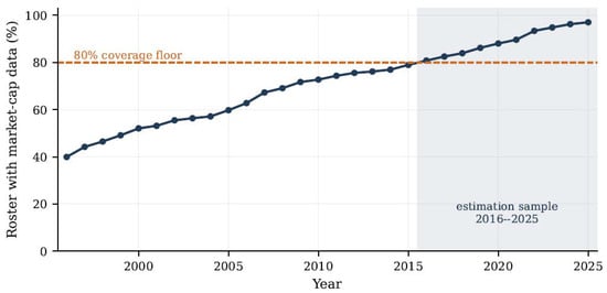
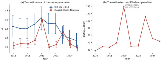
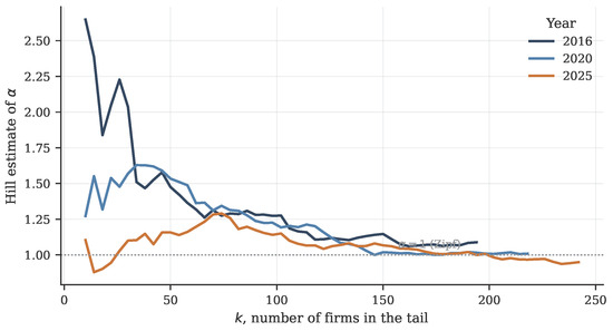
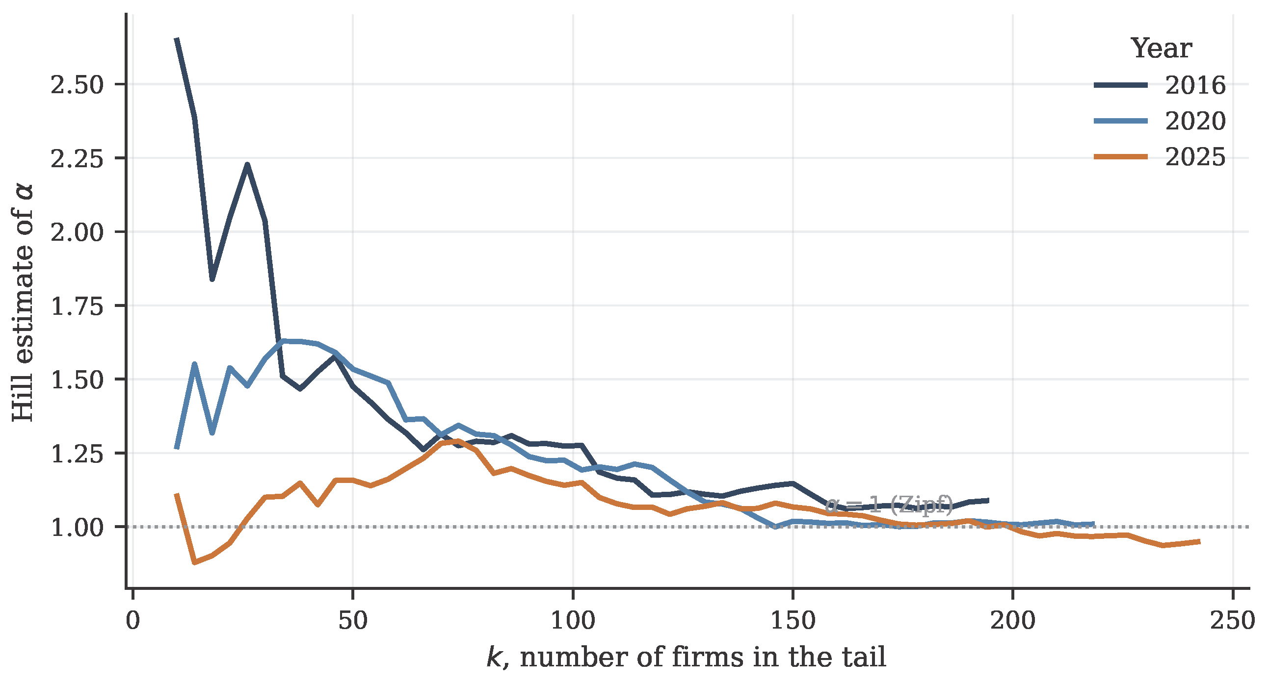
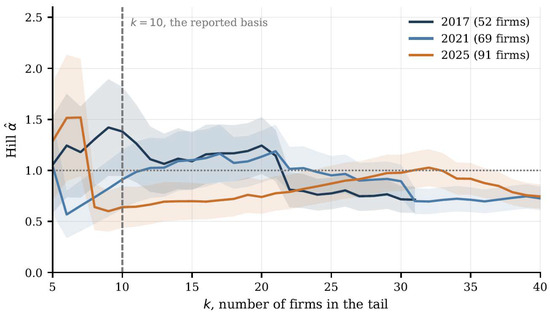
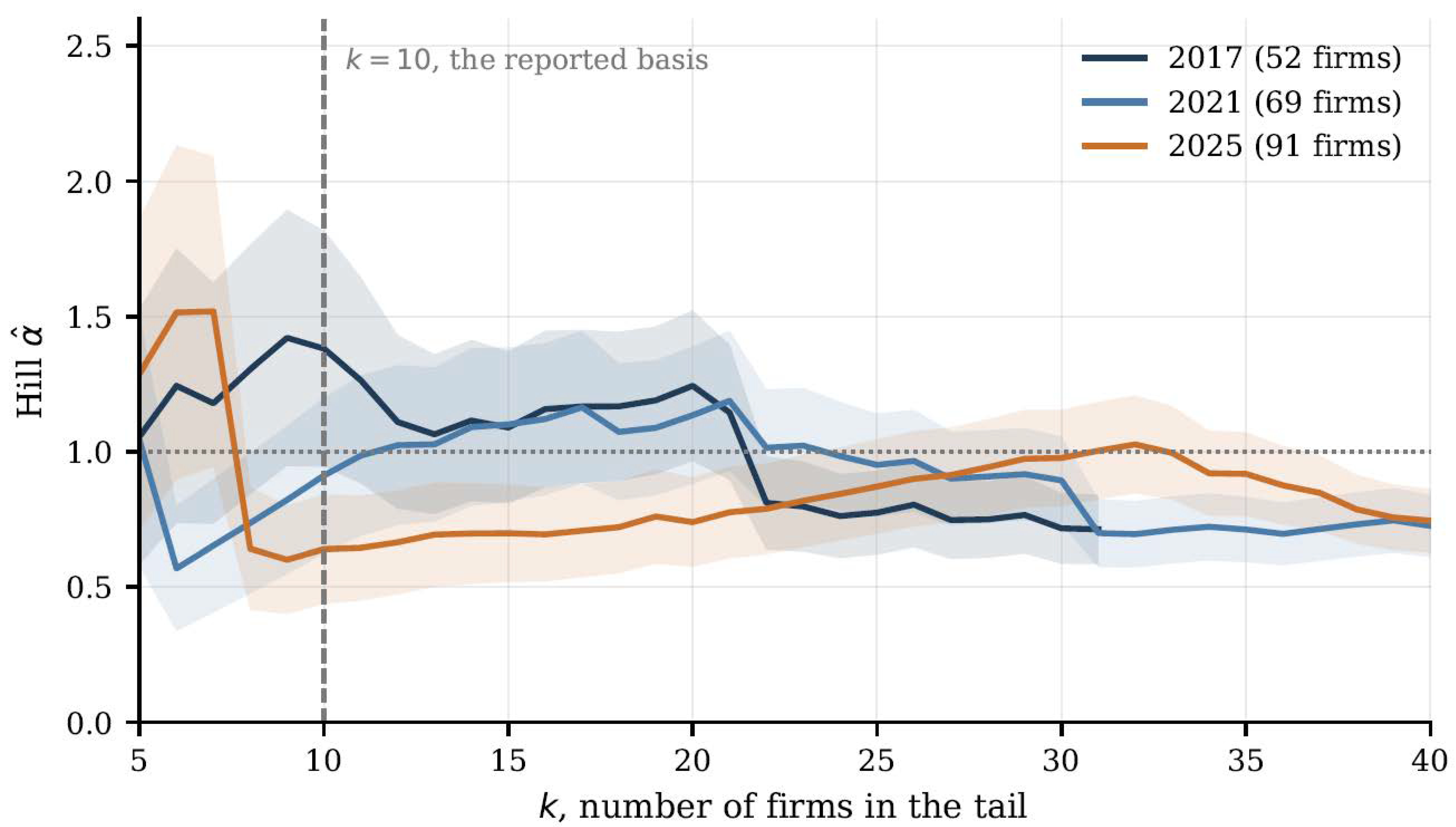
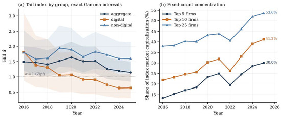
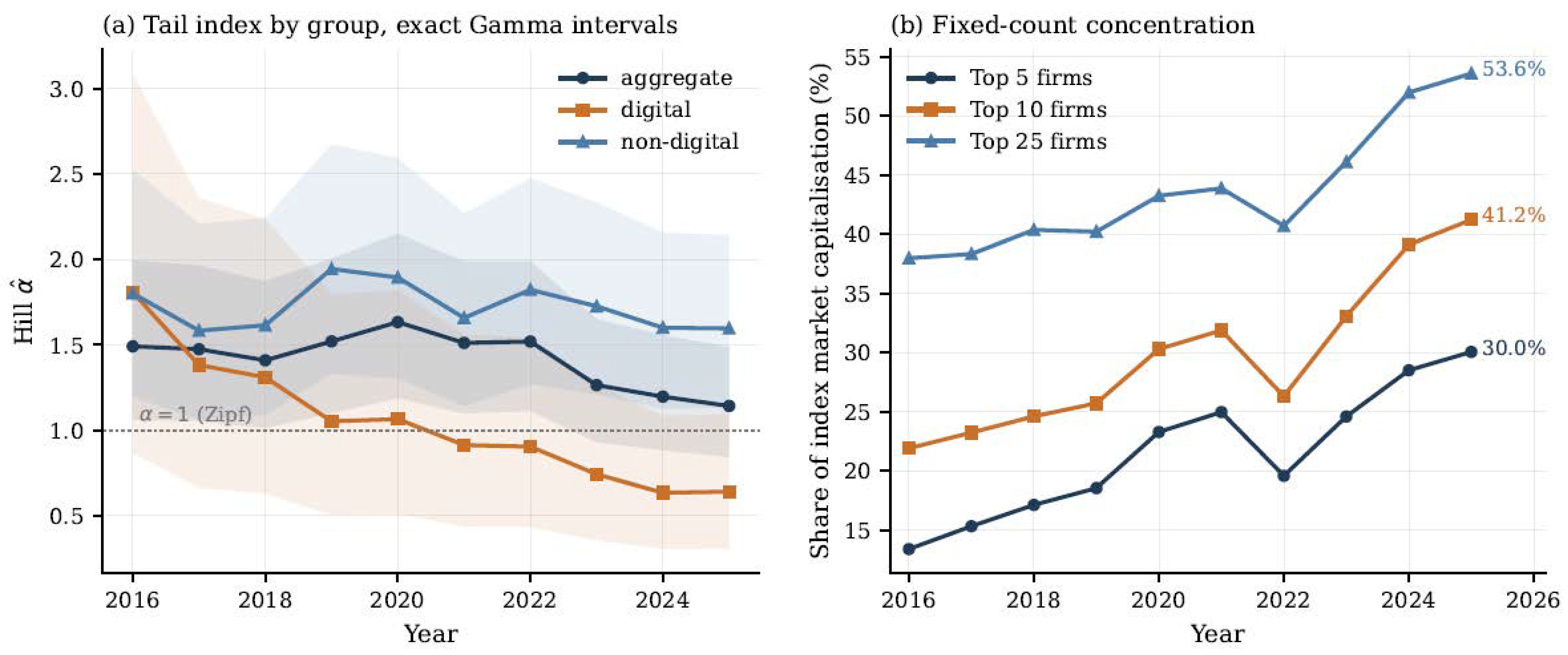
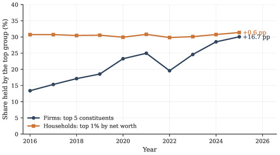
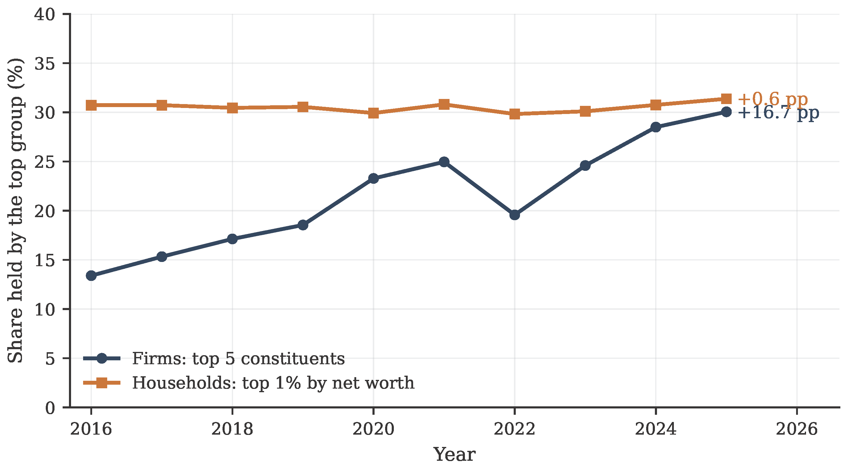

Disclaimer/Publisher’s Note: The statements, opinions and data contained in all publications are solely those of the individual author(s) and contributor(s) and not of MDPI and/or the editor(s). MDPI and/or the editor(s) disclaim responsibility for any injury to people or property resulting from any ideas, methods, instructions or products referred to in the content. |
© 2026 by the authors. Licensee MDPI, Basel, Switzerland. This article is an open access article distributed under the terms and conditions of the Creative Commons Attribution (CC BY) license.