


Abstract
An implied volatility surface is typically rebuilt each day from that day’s quotes alone, even though the quotes missing on a given day were usually traded the previous day. We treat a panel of daily surfaces as frames over moneyness, maturity and calendar time—a video-completion view—and reconstruct a target day’s missing region from the surrounding days. The model propagates along the three axes separately, mixes them by a gate reading which nodes are absent, and learns only a correction to a classical single-day fit. Using S&P 500 index options from January 2010 to August 2025, we score against strictly held-out market quotes. When an entire wing is withheld, the reconstruction beats a cross-sectional benchmark by 27.1%; holding the architecture fixed and varying only the input window shows that nine days of context rather than one accounts for a further 15.0% of the remaining error. Under random withholding, the method does not help, and under an interior expiry withholding it slightly hurts. Temporal information is thus valuable for structured outages, wing outages above all. The completed surface violates static no-arbitrage conditions more often than the benchmark, however, and a projection removing those violations removes most of the accuracy advantage, so it is not yet ready for pricing or risk use.
1. Introduction
An implied volatility (IV) surface is a two-dimensional object—volatility as a function of moneyness and maturity—but the data behind it never arrive as a complete grid. On a typical day, a large fraction of the strike–maturity combinations that a desk would like to price has no reliable quote at all. The gaps are not scattered at random. They sit where liquidity is thin: deep in the wings, at long maturities, and in the stretches between listed expiries. They also persist because the strikes that fail to trade on a day are usually the same ones that failed to trade on the previous day.
The standard response is to fit a smooth surface to each day’s quotes on its own. Parametric families such as SVI and its arbitrage-free variants (Gatheral & Jacquier, 2014; Guo et al., 2016), nonparametric smoothers with no-arbitrage constraints (Fengler, 2009), and more recently neural approximations (Ackerer et al., 2020; Chataigner et al., 2020; Zheng et al., 2021) all share this cross-sectional premise: the information used to fill a hole comes from the same day’s remaining quotes. Where a hole is small and surrounded by data, that premise is sound. Where an entire wing is missing, it is not—there is nothing on the correct side of the surface to interpolate from, and the fit is extrapolating under whatever shape assumption the model happens to carry. Asymptotic moment conditions (Lee, 2004) bound how steeply the wings may grow but say little about their level at the moneyness a desk actually quotes.
Yet, the information does exist. Surfaces move slowly relative to the daily sampling frequency, a fact documented since the earliest work on IV surface dynamics (Cont & da Fonseca, 2002; Gonçalves & Guidolin, 2006; Skiadopoulos et al., 2000). The wing that cannot be observed today was very likely quoted the day before and will be quoted the day after. Filling the hole from the neighboring days is a different problem from fitting today’s cross-section. The natural formulation for it is not surface fitting but video completion: the panel of daily surfaces is a sequence of frames over a grid, the missing region on a target day is a hole in one frame, and the surrounding frames are context.
This paper develops that formulation and, more importantly, asks under what conditions it actually helps. We make four contributions.
First, we pose IV surface reconstruction as spatiotemporal completion on a tensor and build a model, VolPaint, around three properties the financial problem demands. The three axes carry different structure—smile and skew along moneyness, term structure along maturity, market-state persistence along calendar time—so the model propagates along each separately and mixes them with a gate that reads the missingness pattern. The network never invents an entire surface: a classical single-day fit supplies a baseline and only the correction inside the hole is learned. Observed quotes are returned unchanged by construction, so a completion never overwrites a price the market actually made. The block’s advantage over a generic three-dimensional network is measured under both evaluation protocols in Section 4.6.
Second, we isolate the contribution of temporal context in a way that earlier comparisons of temporal against single-frame models cannot. Comparing a video model to a single-frame model changes both the architecture and the input window at once, and the resulting gain cannot be attributed to either. We instead run the identical architecture, parameter count, loss, training dates and mask realizations twice, varying only whether the model sees nine frames or one. Against a controlled reference, the nine-frame model reduces error by between 18% and 59% depending on the missingness family, with hierarchical confidence intervals that exclude zero in all seven cases. Repeating the same isolation against strictly held-out market quotes gives 15.0% in the wings with a nine-day window and 23.4% with a five-day one, nothing on a random holdout, and a small negative on an interior expiry.
Third, we score every claim under two protocols and report where they disagree. The first uses a smooth model-fit reference surface as the target, which is what most of the surface completion literature does; the second holds out real traded quotes, keeps their values and their coordinates out of the model input, and scores only at those coordinates. The two protocols rank models differently. Under the controlled reference, our finance-aware propagation block beats a parameter-matched generic three-dimensional convolutional network on six of seven tasks; against traded quotes that margin collapses and, on one task, reverses. A fitted reference is partly a record of the fitting procedure, so a model can score well on it by learning that procedure rather than the market. We treat the controlled protocol as an upper bound and report the strict protocol as the result.
Fourth, and most consequentially for practice, the strict result is conditional. Temporal context does not improve implied volatility surface fitting in general; it adds value when the same-day cross-section is structurally uninformative about the missing region, and a benchmark built on random deletion cannot see this, because random deletion never produces such a region.
Where a full wing is held out, temporal context reduces reconstruction error by 27.1% against a strong cross-sectional baseline scored on identical coordinates. Where quotes are held out at random, it does not help, and on some metrics is slightly worse. The pattern indicates where the information is. When quotes are removed at random, each hole retains close neighbors on the same day and same-day interpolation is already close to optimal, so yesterday’s surface adds a stale signal to a well-posed problem. When an entire wing is gone, the same-day neighbors are all on the wrong side, and the previous day’s wing is the only observation of that region. Temporal context substitutes for cross-sectional information where the cross-section is structurally uninformative, and random holdouts, the default benchmark, cannot detect the distinction.
Figure 1 states the mechanism on real data. The remainder of the paper is organized as follows. Section 2 places the work in the literature. Section 3.1 describes the option data and the contract filters, Section 3.2 the grid and the representation, Section 3.3 the two evaluation protocols and Section 3.4 the offline and causal input windows; Section 3.5 defines the missingness families, and the rest of Section 3 the model and the inference procedure. Section 4 reports results. Section 5 discusses what the conditional finding implies and what the study does not establish, and Section 6 concludes.
Figure 1.
Why calendar time carries information a single day does not. All six panels are rendered from the same S&P 500 panel, over nine consecutive trading days centered on 1 November 2022. Panels (a–c) show three frames of the surface video; on the target day t the left wing has been cut away, and the crimson band on the neighboring days marks the same region, which is quoted there. The hole spans every maturity and persists for several days, so no same-day neighbor lies inside the missing wing. Panels (d–f) show what fills it: the cross-sectional anchor, which must extrapolate the wing from the same day alone; VolPaint, which borrows the wing geometry from adjacent days; and the reference surface. All six panels share one vertical scale. Surface color indicates the level of implied volatility, from purple (low) to yellow (high).
2. Related Literature
2.1. Cross-Sectional Surface Construction
Constructing a surface from a day’s quotes is a mature problem. Since Black and Scholes (1973) made implied volatility a meaningful quantity and Dumas et al. (1998) documented the empirical failure of deterministic volatility functions, the literature has developed in two directions. Parametric families impose a shape and fit its parameters: SVI and the arbitrage-free characterizations of Gatheral and Jacquier (2014) and Guo et al. (2016) are the standard, Gatheral (2012) gives the practitioner treatment, and stochastic volatility models such as Heston (1993) generate surfaces whose empirical performance was assessed by Bakshi et al. (1997) and Christoffersen et al. (2009). Nonparametric methods trade shape restrictions for smoothness penalties, with Fengler (2009) providing arbitrage-free smoothing via constrained splines and Fengler (2005) a book-length treatment. Neural approximations are more recent: Ackerer et al. (2020) smooth the surface with a network anchored on a parametric prior, Chataigner et al. (2020) learn local volatility subject to no-arbitrage penalties, Zheng et al. (2021) embed financial constraints in the architecture, and Bergeron et al. (2022), Ning et al. (2023), Cont and Vuletić (2023) and Vuletić and Cont (2024) encode or generate surfaces with latent variable and adversarial models.
What unites this work is that reconstruction on a given day uses only that day’s data. That is the right formulation when the target is a well-posed interpolation, and Section 4.5 measures several of these constructions on our held-out quotes. It is also the assumption we relax.
2.2. Dynamics of the Surface
That IV surfaces evolve smoothly is well documented. Cont and da Fonseca (2002) decompose surface variation into a small number of principal components with strong persistence; Skiadopoulos et al. (2000) and Gonçalves and Guidolin (2006) document predictable structure in the daily evolution of the S&P 500 surface; Fengler et al. (2007) model that evolution through a dynamic semiparametric factor model. Andersen et al. (2015) recover latent states from option panels econometrically, and Carr and Wu (2009) exploit the panel dimension for variance risk premia. This literature establishes the premise our model rests on. The difference from it needs stating exactly, because the two problems look alike and are not. The dynamics literature takes a complete surface on each day as given and asks how the sequence evolves: which factors move, how persistent they are, and whether tomorrow’s surface can be forecast from today’s. Its output is a description or a forecast of a whole surface. The question here runs the other way. Today’s surface is the incomplete object; the neighboring days are complete, or nearly so, in the region that is missing today; and the task is to carry that region across rather than to forecast. The target is therefore a region of the present day, scored at held-out quotes of that day rather than at a future horizon. The neighboring surfaces serve as context on both sides of the target in the offline setting, which no forecasting model does. And the value of the context depends on what the present cross-section already knows, a dependence with no counterpart in forecasting, where the target day’s cross-section is never available. Temporal persistence is treated here as an imputation resource rather than as a forecasting target, and none of the models in this literature are set up to be used that way.
2.3. Learning and Completion
Machine learning in asset pricing is now standard (Almeida et al., 2023; Gu et al., 2020), and volatility modeling in particular has adopted deep networks for calibration (Cuchiero et al., 2020; Horvath et al., 2021). Our architectural vocabulary comes from image and video completion, where the treatment of missing inputs has been studied carefully: partial convolutions (Liu et al., 2018) and gated convolutions (Yu et al., 2019) make the network aware of which pixels are valid, joint spatial–temporal transformers (Zeng et al., 2020) borrow content across frames, and simple separable architectures (Gao et al., 2022) remain competitive for video prediction. Recurrent convolutional models (Shi et al., 2015) and the U-Net (Ronneberger et al., 2015) provide our deep baselines.
We adapt rather than transplant. Three elements of VolPaint are taken from this literature with little change: the use of an explicit observation mask as an input channel, the residual formulation in which a network predicts a correction to a baseline rather than a level, and hard consistency, which returns observed values unchanged—all standard in inpainting. Three elements are ours. The baseline being corrected is a classical financial interpolant rather than a learned one, so that the untrained model coincides with a method a desk already uses. The propagation block of Section 3.7 is built for the fact that an implied volatility surface is not isotropic. Moneyness carries the smile and its skew, maturity the term structure, and calendar time market-state persistence; a single three-dimensional kernel mixes all three through one shared receptive field, where the block keeps them separate and lets a gate that reads the missingness pattern decide how to weight them. Additionally, the evaluation—structured missingness families drawn from how quotes actually go missing, scored against strictly held-out traded quotes rather than a fitted target—is new to this setting and, as Section 4.6 shows, changes the answer.
3. Materials and Methods
3.1. Data and Contract Filters
The sample is S&P 500 index options from OptionMetrics (New York, NY, USA), obtained through Wharton Research Data Services (Philadelphia, PA, USA), covering 4 January 2010 to 29 August 2025—3939 trading days, a little under sixteen years. Both the AM-settled SPX and the PM-settled SPXW series are retained; the settlement convention is recorded but not used to exclude contracts, since excluding SPXW would remove most of the short-dated surface.
Contract filters are applied in a fixed order and were frozen before any test-period result was examined. A contract is retained when it is flagged as an index option, when the bid and ask are both present, and when the quote is neither crossed () nor priced at a non-positive mid. Four further rules remove quotes carrying no usable volatility information. The bid must be at least $0.05, which drops the near-worthless deep wings whose implied volatilities are numerically unstable. The relative spread must not exceed 1. Days to expiry must lie between 7 and 365, which excludes the last week before expiry, where implied volatility is dominated by discreteness. Additionally, a quote is dropped when it is stale by more than five trading days, measured as the gap between the quote date and the last date on which the contract traded. No minimum volume or open-interest filter is imposed: doing so would delete precisely the thin-liquidity regions pertaining to this paper and would make the missingness patterns endogenous to the filter.
For each expiry, we keep only out-of-the-money contracts, puts below the forward and calls above it, which is the standard splice and is a deterministic function of moneyness alone. The forward is recovered per expiry from put–call parity rather than from a dividend series. For every strike quoted as both a call and a put, is linear in K, so a least-squares line through the matched mids returns the discount factor as its slope and the forward as the ratio of intercept to slope. An expiry with fewer than four matched strikes is dropped rather than assigned a forward from a curve, so every retained quote sits on a forward its own expiry implies. Duplicate SPX/SPXW quotes at the same strike and expiry are averaged before matching. Implied volatilities are OptionMetrics’ own, computed from the mid, and are retained only when finite and inside ; log-forward moneyness is retained on , generously wider than the grid, so no quote is lost at the grid boundary before the grid is applied. A day with fewer than 200 surviving quotes is dropped entirely. Each quote carries a liquidity weight , winsorized at the 1st and 99th percentiles and normalized to sum to one; this weight enters the objective under the strict protocol and the vega-weighted error metric, and nothing else.
Corporate actions do not arise for an index option, and no split or dividend adjustment is applied to strikes.
3.2. Grid and Representation
Reconstruction is performed on a fixed grid of 21 log-forward-moneyness nodes and nine maturities calendar days, giving 189 nodes per day.
Quotes and grid nodes are distinct objects, and the distinction matters for what “missing” means. A grid node is supported on a given day when at least one retained quote lies within a scaled distance of of it, moneyness measured in units of the grid step and maturity in units of in . That metric puts the two axes on a comparable footing since strikes are quoted far more finely than expiries. Where several quotes fall inside that radius, the nearest is used, so no averaging blurs the fine structure the wings carry. A node with no quote inside the radius is unsupported, and the observation mask M that the model receives is exactly the support indicator. An unsupported node is not a missing measurement to be imputed and scored; it is a coordinate at which the market produced no price, and under the strict protocol nothing is ever scored there.
Quote support on this grid is 63.9% over the full sample and is markedly asymmetric across moneyness: the at-the-money column is supported on 79.7% of days, the leftmost column on 73.2%, and the rightmost column on only 15.7%. Over the test period support is higher, 87.1% overall, but the asymmetry remains, with 97.7% in the five leftmost columns against 55.9% in the five rightmost. This asymmetry is a fact about the market, and we return to it in Section 4.6 (“Is the Wing Result an Artifact of Thin Support?”) because it bears directly on how wing results should be read.
Splits are chronological and fixed in advance: training covers 4 January 2010 to 31 December 2019 (2516 days), validation 2 January 2020 to 31 December 2021 (505 days), a calibration buffer 3 January to 30 June 2022 (124 days), and the untouched test period 1 July 2022 to 29 August 2025 (794 days).
The model works in standardized log total variance. Writing for total variance at node , the representation is
with and the mean and standard deviation of at node over the 2516 training days. Both are arrays, one value per grid node, computed once from the fitted reference surfaces of the training period and never re-estimated on later data, and they are statistics of total variance alone. The forward price enters only through the moneyness coordinate that places a quote on the grid, not through or . Total variance rather than volatility is the natural quantity because calendar arbitrage is a monotonicity condition on w along ; the logarithm keeps it positive; the node-wise standardization prevents the short-dated wings, which are an order of magnitude more variable than the at-the-money term structure, from dominating the loss. Predictions are mapped back by , and all reported errors are in volatility points on that scale.
3.3. Two Evaluation Protocols
Reconstruction quality can only be measured against something, and the choice of that something turns out to matter more than any modeling decision in this paper. We use two protocols and report both.
Protocol A, controlled reference. On quote-rich days a smooth reference surface is fitted to all available quotes with a penalized spline anchored on an SVI-type parameterization. An artificial mask is then applied, the model sees only the retained nodes, and the reconstruction is scored against the fitted reference on the masked nodes. This is the protocol under which most surface completion methods are evaluated. It has two virtues: the target is defined at every grid node, so masks of any shape can be applied, and the comparison is exactly controlled. It has one serious defect, which we quantify in Section 4.6: a reconstruction can be accurate about the fitting procedure rather than about the market. Protocol A is an upper bound, not a proxy for Protocol B.
Protocol B, strict real held-out quotes. Twenty percent of a day’s genuine quotes are held out. Neither their implied volatilities nor their coordinates enter the model input; the observation mask handed to the model is built only from the retained support; and scoring happens only at the held-out quote coordinates, against traded implied volatility. Nothing about the held-out set is visible to the model, and no interpolation onto a grid target intervenes between the prediction and the market. Three holdout designs are used: random, removing 20% of quotes uniformly; wing, removing the quotes beyond a moneyness threshold; and interior expiry, removing an entire listed expiry from the interior of the term structure. The random and wing designs yield 790 eligible test days and the expiry design 732, the latter being smaller because a day needs an interior expiry with enough quotes to remove.
The eligible count differs slightly between the protocols. Protocol A requires the whole nine-day clip to lie inside the test split, because the target is the fitted reference surface for every frame, which leaves usable centers. Protocol B needs only that the clip not run past the end of the panel, since its context frames are built from quotes rather than from fitted surfaces and the scored quantity lives on the target day alone; that leaves 790. For the first eight test days, the context window reaches back into the calibration buffer of the first half of 2022, which the model never trains on and never scores against.
The cross-sectional reference under Protocol B is a set-based attention model that predicts implied volatility at an arbitrary query from the nearest retained quotes, with learned relative-position encoding and an inverse-distance-weighted neighbor mean as its own anchor. It operates on raw quotes rather than a grid, so it is not handicapped by the discretization, and Section 4.5 shows that on pointwise reconstruction it is far stronger than the standard parametric constructions, which is why it serves as the benchmark. We refer to it as the cross-sectional anchor throughout.
3.4. Offline and Causal Windows
Two input windows are used throughout. Because the practical claim of this paper concerns live use, the dates each one sees are set out exactly. The offline window is the nine frames , with the target day at the center; it is the natural setting for marking a historical book or building a research panel, where later days are available. The causal window is the nine frames , with the target day last; no date after t enters the input at any point, so it is the setting a desk faces in real time. Both windows are nine frames, so the two differ in which dates they use and not in how much context they carry. Algorithm 1 sets out the whole procedure for one trading day.
Neither window sees anything about the held-out set. The held-out implied volatilities are absent from every frame, their coordinates are absent from every mask, and the mask on the target day is constructed only from the quotes that were retained. Context frames are built from all of day ’s retained quotes, which are that day’s genuine market data and are never part of the scored set. Test-period parameters are never fitted: the network weights, the standardization constants of Equation (1), and the cross-sectional benchmark’s parameters are all fixed before the test period begins.
| Algorithm 1: The strict evaluation protocol for one trading day as executed |
Input: trading day t; its retained quotes; holdout design ∈ {random, wing, interior expiry}
|
3.5. Structured Missingness
Random masks are the default in completion benchmarks and are the wrong default here because real gaps are shaped by liquidity. We define seven families, shown in Figure 2, all applied on the target frame of a nine-day clip.
Figure 2.
The seven missingness families, generated by the same code the experiments use. Crimson marks nodes missing on the target day. A dashed frame marks the three persistent families, where the same region is also absent on the neighboring days, so the outage is a spatiotemporal tube rather than a hole in a single frame.
Random removes each node independently with probability . Block removes a contiguous rectangle at a random position, 18 of 189 nodes. Wing removes the five columns beyond on one side, alternating side by realization, 45 of 189 nodes across all maturities. Maturity band removes two adjacent maturities across all moneyness, 42 of 189 nodes. The three persistent families—persistent block, persistent wing and persistent maturity—remove the same region on five consecutive frames rather than one, so the missing region is a spatiotemporal tube and no same-day or adjacent-day observation lies inside it. Persistent masks are the demanding test for a temporal model: they remove exactly the information the model would most like to borrow.
How these designs compare with the gaps the market actually produces is an empirical question about the panel, and Table 1 answers it for the test period. On the left, quotes reach the grid edge on every test day: no day has even one unsupported left-edge column. On the right, gaps are the norm. The rightmost columns are unsupported on 83% of test days, the gap is two columns wide at the median and four at the 90th percentile, and once a right-wing column loses support it stays unsupported for two days at the median, five at the 75th percentile and twelve at the 90th. The synthetic wing of Protocol A, five columns wide, is therefore wider than all but 1% of real right-wing gaps; the strict wing holdout of Protocol B, which removes the deepest 20% of a day’s quotes, is comparable in share of the surface to a four-to-five-column gap. Both designs sit at the severe end of what the market produces on the right and beyond anything it produces on the left. The one-day persistence of the main results matches the median real spell; the longer spells that make up the upper quartile are examined in Section 4.7.
Table 1.
Right-wing gaps in the test period as the market produced them, measured on the grid. A column counts as unsupported on a day when at least half of its maturities have no quote within the support radius of Section 3.2. The left edge had no unsupported column on any test day.
3.6. Baseline-Anchored Residual Completion
The first component, which we call baseline-anchored residual completion (BARC), fixes what the network is allowed to change.
Let denote the target-day surface in the representation of Equation (1) and the observation mask, with where a node is observed. A classical single-day fit is computed for every frame of the clip by Clough–Tocher triangular interpolation (Renka & Cline, 1984) of the observed nodes in total-variance space, with nearest-neighbor fallback wherever the cubic interpolant is undefined or non-positive—total variance must be positive, and cubic interpolation can overshoot inside a large hole. Observed nodes are retained exactly, so agrees with the data wherever data exist.
The network predicts a correction rather than a surface. Let be the decoded feature map at the target frame, an array of C values at each of the grid nodes produced by the network of Section 3.7. Two functions map to a single value per node, and both are convolutions: the value at a node is a weighted sum of the C entries of at that node and at its eight neighbors on the grid, with one set of weights shared across all nodes and fitted by the optimizer. The first, , is the residual—the proposed correction to the anchor at each node, in the representation of Equation (1). The second, , is a gate logit: an unbounded real number per node that the logistic function maps to . The gate multiplies the residual node by node, so the network can scale its correction down to nothing where the anchor is already adequate and leave it at full strength where the anchor is not. Then
where ⊙ is elementwise multiplication, is the logistic function, are the observed values, and is the unconstrained completion before the consistency step. The two agree on the missing set and differ only where a quote exists. Two properties follow directly. The first term enforces hard observation consistency: at nodes where the market quoted a price, the output is that price, so the observed-node reconstruction error is exactly zero rather than small. The second term makes the model a correction to a classical fit: the residual head is initialized at zero, so at the start of training the network reproduces the interpolant exactly and learns only where it needs to deviate. This matters in the wings, where an unanchored network has to invent a level as well as a shape. The gate lies in but the residual head is unbounded, so Equation (2) does not by itself limit how far may travel from ; what discourages large excursions is the zero initialization and the penalty in Equation (7). A hard guarantee would require a bounded residual or an explicit projection, neither of which we impose.
3.7. Finance-Aware Tri-Axis Propagation
This section describes the network that produces in Equation (2).
Inputs. Each frame of the clip carries three channels, each a array on the grid: the anchor B in the representation of Equation (1), the observation mask M, and the observed residual , where is the value the market actually quoted at a supported node. The content of that third channel depends on the protocol. Under Protocol A, the anchor is the interpolant of Section 3.6, which reproduces the observed nodes exactly, so wherever and the channel is identically zero: the network sees two informative channels, not three. Under Protocol B, the anchor is the cross-sectional fit of Section 3.3, which does not pass through the retained quotes, and the channel carries the gap between the smooth fit and the nearest traded quote at each supported node, with a mean absolute value of in the representation of Equation (1) and a standard deviation of . The channel is kept in both cases so that one network definition serves both protocols.
Feature maps. A convolution replaces each grid value by a weighted sum of its neighbors, with weights that are learned rather than fixed; a channel is one such set of weights, and applying C of them to the same input gives C different filtered copies of the surface, called feature maps. The three input channels are first passed, one frame at a time, through two convolutions with output channels each (the encoder). The result is a tensor : 112 feature maps for each of the frames, each map a array over . The width is a tuning choice with no financial meaning, fixed on the validation split along with the other settings listed in Appendix A.
Propagation. The block we call finance-aware tri-axis propagation (FTAP), Figure 3, moves information through z along one axis at a time. Let denote a one-dimensional convolution of length m applied along the moneyness axis to every channel separately, with and the same along maturity and calendar time; each such operator has just m weights per channel. The three directional responses are
Here are matrices applied at every grid cell and frame independently (a convolution); they let the channels exchange information after the directional filtering but do not mix neighboring cells, and their entries are fitted by the optimizer. Using kernel lengths 3 and 5 on each axis gives every direction both a local and a wider view at a small fraction of the parameters a full kernel would need.
Figure 3.
The tri-axis propagation block. Three depthwise branches propagate along moneyness, maturity and calendar time separately, and a gate driven by the pooled features and the missing fraction decides how much weight each direction receives, so the mix adapts to the shape of the outage rather than being fixed by the architecture.
Gate. How the three directions should be combined depends on what is missing. A hole in the wings should be filled mostly from calendar time, because the same-day neighbors are on the wrong side of the smile; a scattered random hole should be filled mostly from its immediate surroundings. The block therefore chooses the mix from the data. Let denote the average of each channel over all positions, so summarizes the clip in one number per channel, and let
be the fraction of the clip that is missing. The two are concatenated into a vector and passed through a small multilayer perceptron (MLP). An MLP is a composition of affine maps and elementwise nonlinearities whose coefficients are fitted by the optimizer; this one has two layers. The first computes with and , where , the standard normal distribution function, is applied to each entry and lets the map bend. The second computes with and , giving three unbounded scores, one per axis. A softmax, , turns the scores into positive weights that sum to one,
The output is one triple of weights per clip, so the gate decides, for the outage at hand, how much of the update should come from each axis.
Block output. The weighted directional responses are mixed across channels by a further matrix , normalized, and added back to the input,
where is group normalization (Wu & He, 2018), a rescaling of each group of channels to unit variance that keeps training stable. The additive form means each block refines z rather than replacing it. Five such blocks are stacked, and the target frame’s slice of the result passes through one more convolution (the decoder) to give . Two final convolutions with a single output channel produce the residual and the gate logits of Equation (2). Appendix A gives the parameter count by component.
What differs from a generic 3D CNN. The parameter-matched anchored three-dimensional network of Section 3.9 is identical in every respect but one: its five blocks each apply a single convolution that mixes moneyness, maturity and time through one shared kernel, where FTAP applies Equations (3)–(6). The anchor, the hard consistency step, the zero-initialized residual head, the encoder and decoder, the loss and the training recipe are the same. The comparison in Section 4.6 therefore isolates the propagation block.
3.8. Objective and Training
The network of Section 3.7 ends in ; Equation (2) turns into the unconstrained completion and the consistent one ; the objectives below say how far those are from what the market did, and the optimizer adjusts every parameter listed in Section 3.7 to reduce that distance. The two protocols supervise different things, so the objective differs accordingly: under Protocol A, the completion is scored on the grid, while under Protocol B this occurs at quote coordinates after the interpolation of Equation (8).
Both objectives are written for a minibatch of target days. Under Protocol A, a target is defined at every grid node, so the loss runs over the masked nodes. Let be the missing set of day t, the Huber loss and the map back to volatility points. Observed nodes are returned unchanged by Equation (2) and contribute nothing, so
with and . The first term is the reconstruction loss in the standardized representation; the second states the error in the units a practitioner reads, so the objective does not become indifferent to the wings after standardization; the third is a weak pull toward the classical fit that discourages large excursions where the data are silent.
Under Protocol B no such target exists. A node with is either a held-out quote or a strike–maturity pair the market never quoted, and the second kind has no observable value to compare against, so is not a usable supervision set. Supervision instead comes from the held-out quotes themselves. Write for the set of quotes held out on day t, each with traded implied volatility at coordinates and liquidity weight . The prediction at a quote coordinate is the cross-sectional anchor’s own value plus the model’s grid-level correction interpolated to that coordinate,
with bilinear interpolation from the grid to . Carrying the correction rather than the level keeps the anchor’s full strike resolution, which the grid would otherwise destroy. The interpolation uses the unconstrained field rather than : imposing grid-node consistency before interpolating would fold the quote-to-grid aggregation error into the correction and destroy the property that an untrained model reproduces the anchor exactly. The objective is then
with and . The first term is summed within a day and averaged across the batch, so a day with more held-out quotes carries more weight and liquid quotes dominate within it; the second and third are pooled across the batch and normalized by the total count, so no single day dominates them. The robust term keeps a handful of high-vega quotes from defining the whole correction, and the third term is the same pull toward the classical fit as before—the only term evaluated on the grid since it needs no target.
The Huber loss uses a transition threshold of in the units of its argument, which is the standardized representation for and volatility points for . Optimization is AdamW with weight decay , a cosine-annealed learning rate over the full run, and gradient-norm clipping at ; the learning rate is with batch size 48 under Protocol A and with batch size 24 under Protocol B, the smaller step reflecting the noisier quote-level objective. Protocol A runs 25 epochs and Protocol B runs 30. There is no early stopping: every run completes its epoch budget, and the retained checkpoint is the epoch with the lowest mean validation error across the mask families under Protocol A and across the holdout designs under Protocol B. The test period is never consulted in selection.
Hyperparameters were fixed on the validation split before the test period was opened, and were not tuned per mask family, per holdout design or per seed. The channel width (112), block count (5), kernel lengths (3 and 5), clip length (nine frames) and loss weights are common to every experiment reported here; the clip-length sweep of Section 4.7 is the one place where a structural choice is varied, and it is reported rather than used for selection. Both arms of every paired ablation were run on the same hardware; the computing environment is recorded in Appendix A.
3.9. Baselines
Under Protocol A, we compare against a single-frame convolutional network of comparable capacity, a generic three-dimensional convolutional network, an anchored three-dimensional network carrying the same baseline contract as Equation (2) and matched in parameter count, a U-Net (Ronneberger et al., 2015), a bidirectional convolutional LSTM (Shi et al., 2015), temporal coordinate interpolation, and a principal component autoregressive smoother. The parameter-matched anchored three-dimensional network isolates the tri-axis propagation block: it shares the representation, the anchor, the hard consistency constraint, the training data and the capacity, and differs only in using an isotropic kernel in place of Equations (3)–(6).
Under Protocol B the reference is the cross-sectional anchor described in Section 3.3, which is scored on identical held-out coordinates.
3.10. Statistical Inference
Daily error differences are strongly autocorrelated, so we use a paired block bootstrap (Künsch, 1989; Politis & Romano, 1994) with blocks of five consecutive trading days and 5000 resamples, in the spirit of the predictive-accuracy comparisons of Diebold and Mariano (1995). For the temporal isolation experiment of Section 4.1, which involves three training seeds, the bootstrap is hierarchical: training seeds and time blocks are resampled jointly over 10,000 replications, so the interval reflects both the sampling variability of the test period and the variability of the training run. Because Monte Carlo resampling cannot produce a p-value below the resolution of the resample count, we apply the add-one correction, so the smallest attainable two-sided raw p-value is for the 5000-replication paired bootstrap and for the 10,000-replication hierarchical one. Multiplicity is handled by the Holm procedure (Holm, 1979) applied within each metric family rather than once across every table in the paper.
3.11. Shape Diagnostics
Three static no-arbitrage conditions are checked on every completed grid, following Carr and Madan (2005). Let be the forward-normalized Black–Scholes call price implied by at node , with strike . Along the strike axis, the call must be non-increasing, , and its slope must be non-decreasing,
which is the butterfly condition written with divided differences, because the strikes are unevenly spaced. Along the maturity axis, the total variance must be non-decreasing at fixed moneyness, , the calendar condition. A cell counts as violating when the relevant difference has the wrong sign by more than for the butterfly and for the other two, and a violation rate is the share of cells violating, averaged over test days. These are diagnostics of the completed grid, not of prices at quote coordinates, and Section 4.10 reports them for every method on identical days.
4. Results
4.1. Isolating Temporal Context
The first question is whether neighboring days carry usable information at all, separately from any architectural advantage. We answer it by running the identical model twice. Both arms use the same architecture, the same parameters, the same loss, the same training and test dates and the same mask random-number stream; the only difference is the length of the input window, nine days against one.
With a single frame the temporal convolutions in Equation (3) see only zero padding on either side, so they reduce to a learned per-channel rescaling of that frame and carry no cross-day information. The nominal parameter count is identical, but effective capacity is not: the off-center taps of the length-3 and length-5 temporal kernels multiply zeros in the arm and receive no gradient, so that arm has fewer usable degrees of freedom along one axis. The design therefore isolates the temporal axis far more tightly than a video-against-single-frame comparison does, but it equalizes the parameter count rather than the effective capacity.
Table 2 reports the outcome over 786 test days and three training seeds. Nine days of context reduce reconstruction error in every family, by 18.0% on persistent block up to 58.8% on wing, and all seven hierarchical intervals exclude zero with Holm-adjusted . The direction is identical in all three seeds for all seven families.
Table 2.
Temporal isolation under Protocol A. Identical architecture, parameter count, loss, dates and mask realizations; only the input window differs. Reconstruction root mean squared error in the standardized representation over 786 test days and three training seeds, with hierarchical 95% confidence intervals over seeds and five-day blocks.
The largest gains are on wing (58.8%) and persistent wing (42.8%), which are exactly the families where the same-day cross-section contains no observation on the relevant side of the surface. The smallest is on the persistent block (18.0%), where the outage is a tube: the missing region is absent from the neighboring frames too, so there is less to borrow. Random sits in between at 25.7%. The same pattern, gains concentrated where the cross-section is uninformative, recurs under the strict protocol.
The vega-weighted error improves in all seven families as well. Forward-normalized price mean absolute error improves in five of seven but not significantly on random or persistent block.
4.2. Model Comparison Under the Controlled Reference
Table 3 places VolPaint against the single-frame network and the parameter-matched anchored three-dimensional network. Against the single-frame model the improvement ranges from 30.6% to 60.4% and every interval excludes zero, though that comparison changes architecture and input window together.
Table 3.
Protocol A reconstruction error on 786 chronological test days, scored only on masked nodes. Improvements are relative reductions in root mean squared error. The parameter-matched anchored 3D network shares the representation, anchor, hard consistency constraint and capacity, and differs only in using an isotropic kernel.
The parameter-matched comparison is more mixed. Tri-axis propagation is ahead on six of seven families, by 26.7% on random down to 5.3% on persistent maturity. On persistent wing, the margin is 2.8% with a 95% interval of roughly and Holm-adjusted : on the hardest family, an isotropic kernel with the same anchor and the same capacity does about as well.
Figure 4 shows one worked wing case. The signed error surfaces share a symmetric scale and are directly comparable; the flat plane over the observed region in every panel is the hard-consistency constraint of Equation (2), and all remaining error is confined to the wing that was removed.
Figure 4.
A worked wing case on a test day. Top row: the masked region in crimson, the cross-sectional anchor, and the VolPaint completion; in (b,c), surface color indicates the level of implied volatility on a scale shared by the two panels, from purple (low) to yellow (high). Bottom row: signed reconstruction errors on one shared symmetric scale, shaded blue where the reconstruction lies below the reference surface and red where it lies above it. The error is identically zero over the observed region in all three panels—this is the hard consistency constraint of Equation (2)—and the remaining error is confined to the removed wing, where it is visibly shallower for VolPaint than for the single-frame model.
We also compared against every other baseline we implemented: a U-Net, a principal component autoregressive smoother, temporal coordinate interpolation, a generic and an anchored three-dimensional network, and a bidirectional convolutional LSTM. VolPaint has the lowest error on all seven families, but two margins are thin. On the wing family, the LSTM reaches 0.008448 and temporal coordinate interpolation 0.008346, against 0.008138, and the advantage over the LSTM does not survive Holm correction. Temporal coordinate interpolation, which borrows the missing region from the nearest day on which it was observed with no learning at all, beats every single-frame network on both wing families. A method with no parameters outperforming a trained single-frame network wherever a wing is missing is a direct indication of where the information lies.
4.3. Strict Real Quotes: A Conditional Result
Protocol A gives a favorable and internally consistent picture. Protocol B does not simply reproduce it, and the difference is the substantive finding.
Table 4 and Figure 5 report reconstruction error at strictly held-out quote coordinates against the cross-sectional anchor, over three training seeds. On the wing holdout, the temporal model reduces error by 24.4% in the offline setting and 27.1% in the causal setting, where only past and current frames are visible. On the random holdout, it is 4.5% and 3.4% worse. On the interior expiry holdout, the difference against the cross-sectional anchor is within noise in both directions, though Section 4.4 shows that the comparison hides a small but real cost of temporal context on that task.
Table 4.
Protocol B: reconstruction error at strictly held-out quote coordinates, in volatility points, mean ± standard deviation over three training seeds. Neither the held-out values nor their coordinates enter the model input. Positive improvement favors the temporal model.
Figure 5.
The conditional result on strictly held-out market quotes. Temporal context helps substantially where an entire wing is absent, does not help where quotes are removed at random, and is indistinguishable from the cross-sectional anchor on an interior expiry. Error bars are standard deviations over three training seeds.
The causal result is not weaker than the offline result on the wing task; it is stronger. A model restricted to past information recovers the missing wing at least as well as one allowed to look forward, which means the gain does not depend on future frames and the method is usable in a live setting. The random-holdout result is negative. When quotes are removed uniformly, every hole retains close same-day neighbors, the cross-sectional problem is well posed, and the additional temporal input contributes a slightly stale signal to a problem that did not need it.
Under a random holdout, the default benchmark in completion work, one would conclude that temporal context does not help. Under a wing holdout, which is what the market actually produces, one concludes the opposite. The two are the same model, the same training run and the same test period.
4.4. Isolating Temporal Context on Real Quotes
Section 4.3 compares VolPaint against a different model, so the wing result there confounds the input window with the architecture and the anchor. Section 4.1 separates the two, but does so under Protocol A, and Section 4.6 shows that Protocol A’s conclusions do not transfer. The temporal isolation is therefore repeated under Protocol B: the same architecture, parameter count, loss, training seeds, training dates and test days, with only the input window changed, scored against strictly held-out market quotes.
Table 5 reports it. On the wing holdout, nine days of context reduce error by 15.0% over one day, with a hierarchical interval of and all nine seed pairings favoring the longer window. On the random holdout, the difference is 0.8% with an interval spanning zero. On the interior expiry holdout, the longer window is 3.1% worse, with none of the nine seed pairings favoring it. Both non-null results sit at the resolution limit of the resampling and survive Holm correction across the three designs at .
Table 5.
Temporal isolation under Protocol B: VolPaint with a T-day window against VolPaint with a one-day window, at strictly held-out quote coordinates, in volatility points. Identical architecture, parameter count, loss, seeds, training dates and test days; only the input window differs. Reductions are relative to the error; intervals resample training seeds and five-day blocks jointly over 10,000 replications. The seed win rate counts the nine pairings of a T-day seed against a one-day seed.
The nine-day window is not what drives this. We repeated the same isolation with three- and five-day windows, again against the one-day model on identical days and seeds. The wing reductions are 17.6% () and 23.4% (), each with all nine seed pairings in favor; the five-day window is the best of the three and the nine-day window the weakest. On the random holdout, the three windows give , and , a scatter around zero; on the interior expiry holdout, they give , and , null at three days and negative beyond. Table 5 carries all three. The conditional structure is therefore not a property of one window length, and the headline is, if anything, understated by the choice of nine days: the informative neighbors are the nearest ones, and a week of context captures what nine days do with less to average over. This is the strict protocol counterpart of the saturation seen under the controlled protocol in Section 4.7.
The wing advantage decomposes. In these runs, the nine-day model beats the cross-sectional anchor by 28.7% in the wings, and that reduction factorizes exactly: the one-day model improves on the anchor by 16.1%, attributable to the single-day architecture and the anchored residual formulation, and the longer window removes a further 15.0% of the error that remains after that first step, with . Expressed in percentage points of the anchor’s error, the single-day model accounts for 16.1 of the 28.7 and the window for the other , or 12.6 points: the 15.0% is a reduction of what the one-day model leaves, and is the same quantity measured against the anchor. Roughly half of the wing advantage is therefore attributable to temporal information rather than to a better single-day model. The conditional structure is also sharper than in Section 4.3. Interior expiry is not merely a task where temporal context fails to help; it is one where it hurts. This is predicted by the substitution reading. An interior expiry has quoted maturities on both sides of it, so the same-day cross-section is informative there, and adding a channel of day-old information to a well-posed interpolation costs accuracy rather than adding to it.
4.5. Classical Surface Constructions on the Same Quotes
The cross-sectional reference used so far is a learned attention model, which is the right control for isolating temporal context but is not a construction the literature would recognize as the standard. Table 6 therefore adds three that it would—per-slice SVI (Gatheral & Jacquier, 2014), SSVI (Gatheral & Jacquier, 2014) and eSSVI (Hendriks & Martini, 2019)—each fitted to the retained quotes of every test day and scored at the identical held-out coordinates, across all 790 days and three training seeds, with moving-block bootstrap intervals.
Table 6.
Strict protocol, all 790 test days: classical surface constructions fitted to each day’s retained quotes and scored at the identical held-out coordinates. Error is in volatility points with a moving-block bootstrap interval; violation rates are measured on a dense grid evaluation of the fitted surface. VolPaint rows average three training seeds.
The result is a clean separation between two things that are easy to conflate. On pointwise accuracy, the parametric surfaces are not close: on the wing task per-slice SVI reaches 1.67 volatility points, eSSVI 2.97 and SSVI 3.44, against 0.60 for the attention anchor and 0.44 for the causal completion. The ordering is the same on the other two designs. This is what a low-parameter global fit costs when it is scored quote by quote, and it is why the attention anchor serves as the benchmark for reconstruction accuracy.
On shape consistency, the ordering reverses completely. SSVI and eSSVI produce essentially no butterfly violations—the convexity-in-strike condition of Carr and Madan (2005)—which is what their parameter restrictions are for (Gatheral & Jacquier, 2014; Hendriks & Martini, 2019); per-slice SVI produces almost none; the attention anchor produces 4.15% on the wing task and the completion 12.87%. Neither family dominates. The parametric constructions buy static arbitrage freeness at an order of magnitude in pointwise error, and the nonparametric ones buy accuracy at the cost of shape conditions that a pricing application would need. Section 4.10 asks what happens when one tries to have both.
4.6. Where the Two Protocols Disagree
Section 3.3 argued that Protocol A is an upper bound rather than a proxy. Figure 6 shows how large the gap is for a single comparison: tri-axis propagation against the parameter-matched anchored three-dimensional network, everything else held fixed, scored under both protocols.
Figure 6.
The same comparison—tri-axis propagation against a parameter-matched anchored 3D network with representation, anchor, capacity and training data held fixed—scored under both protocols. Under the model-fit reference, the finance-aware block leads on six of seven tasks; against traded quotes the margin collapses and reverses on the offline wing task. Positive values favor tri-axis propagation. Blue bars mark positive values and red bars negative ones.
Against the model-fit reference, tri-axis propagation leads on six of seven tasks, by up to 26.7%. Against traded quotes, the same comparison collapses to a few percent and reverses outright on the offline wing task, where the parameter-matched isotropic network is 12.9% better. The architectural claim that Protocol A appears to support does not survive Protocol B.
Two mechanisms account for the gap.
The first is that the reference moves less from day to day than the market does. This does not follow from the construction—each day is fitted independently, and nothing couples consecutive days—so we measured it. Over the test period, at every grid node carrying a real quote on two consecutive days, the day-over-day change in log total variance has mean absolute size for the reference against for the nearest traded quote, an attenuation of about 11% across 137,697 node-days, with the two changes correlated at . The reference is therefore easier to predict from neighboring days than the market is, though by a modest margin.
The second part is larger and has nothing to do with time. Under Protocol A, the target at a masked node is itself a smooth function of the retained quotes on the same day, because the fitting procedure produced it from them. Part of what any model recovers under Protocol A is therefore the fitting rule rather than market information, and a model with more capacity to represent that rule scores better without being any more informative about prices. Real quotes carry idiosyncratic microstructure that no amount of context recovers, so under Protocol B the margin shrinks toward what the signal actually supports.
Surface completion results reported only against fitted reference surfaces are therefore upper bounds. The strict numbers of Section 4.3 are the result of this paper; the controlled numbers decompose where the gain comes from.
Is the Wing Result an Artifact of Thin Support?
Section 3 noted that quote support over the test period is 97.7% in the five leftmost columns and 55.9% in the five rightmost. Under Protocol A, reference values in the right wing are therefore substantially extrapolated by the fitting model rather than pinned down by quotes, which invites the objection that the wing result measures how well the network has learned the reference model’s extrapolation rule rather than anything about the market.
The objection is testable because the wing mask alternates sides by realization. Splitting the Protocol A wing results by side gives a reduction of 61.2% on the left wing () against 52.8% on the right (), with 54.3% overall. The gain is larger on the well-supported side, which is the opposite of what the extrapolation-mimicry explanation predicts. Together with the strict Protocol B wing result of Section 4.3—scored against traded quotes with no reference surface involved—this makes the extrapolation explanation an unlikely account of the wing finding.
4.7. Information Limits
If neighboring days are the source of the gain, the gain should degrade as the outage lengthens and as the target day becomes emptier. Both hold. A model trained on mixed outage durations and evaluated at one, three, five and ten consecutive days degrades monotonically in every persistent family: on persistent block from 0.00306 to 0.00548, on persistent maturity from 0.00343 to 0.00618, and on persistent wing from 0.00842 to 0.01783, the steepest of the three. The random missing-rate curve behaves similarly, with error rising from 0.0020 at a 10% missing rate to 0.0122 at 70%.
Those numbers are against a reference surface and say only that the error grows; the question that matters is when the completion stops beating the cross-sectional benchmark. Under the strict protocol it does not, within the window we can test, but most of the advantage is gone after the first day. We repeated the wing holdout with the same deepest quotes also removed from the context days nearest the target, so that the outage is a tube rather than a hole in one frame. The causal completion’s advantage over the anchor falls from 27.1% for a one-day outage to 8.0% at three days (), then to 5.9% at five and 5.8% at nine, the last two with intervals of and no further decline. The neighboring days carry the missing wing only while at least one of them still has it; once the outage is longer than the window’s reach the residual gain is what the model extracts from the shape of the surface around the hole, and that is worth about 6% and no more. Set against Table 1, the large gain applies to the half of real right-wing spells that last two days or less, and the small one to the quarter that last five or more.
Clip length behaves less simply. Under the controlled protocol, windows of three, five, nine and fifteen days show no monotone benefit from longer context: three or five days are best on several tasks and fifteen is not reliably better than nine. Section 4.4 finds the same under the strict protocol, where five days beat nine on the wing holdout. Both point to context saturation—the informative neighbors are the nearest ones—and suggest an adaptive temporal horizon as a natural extension.
4.8. Robustness of the Strict Result
We next examine whether the wing result is stable across volatility regimes. Table 7 repeats the paired comparison of Section 4.4 inside quartiles of the prevailing 30-day at-the-money volatility, with the quartile cut-offs taken from the training period so that the split uses no test-period information.
Table 7.
Strict protocol temporal isolation by volatility regime. Regimes are quartiles of 30-day at-the-money volatility with cut-offs fixed on the training period. Entries are the reduction in held-out quote error from nine days of context relative to one, with the architecture held fixed.
The conditional structure holds regime by regime. Temporal context reduces wing error in all four quartiles, by between 11.0% and 21.6%, with no quartile close to zero. It does nothing on the random holdout in any quartile, the range running from to around a null. It is negative on the interior expiry holdout in all four. The gain is largest in the high quartile and smallest in the extreme one, which is consistent with the outage-duration result of Section 4.7: when volatility spikes, the wings that vanish tend to stay missing for longer, and the neighboring days that the model needs are themselves incomplete.
The two wings are not alike: Section 3.2 found quote support of 97.7% on the left of the grid and 55.9% on the right. Holding out the deepest 20% of each side’s own quotes separately, the causal completion improves on the anchor by 15.4% on the left () and by 9.3% on the right (), both at . The gain is robust on both sides, and smaller where the anchor is already struggling: the right wing’s error is three times the left’s (1.06 against 0.37 volatility points), because there are fewer quotes to anchor to on either day. Neither one-sided gain matches the 27.1% of the two-sided holdout, and the difference is informative. Removing both wings at once leaves the same-day cross-section with no deep quotes on either side to interpolate between, which is the most uninformative it can be made, and it is there that temporal context has the most to add.
Where the wing begins is also a choice, and the 20% threshold is arbitrary. Re-running the comparison with the deepest 10% of each day’s quotes withheld gives a gain of 9.0%, with 20% gives 27.1%, and with 30% gives 26.2%. All three are positive, and the gain grows as the withheld region deepens, which is the substitution mechanism appearing in the threshold itself: a shallow wing holdout leaves same-day quotes on the correct side of the smile, so the cross-section is still partly informative and temporal context has less to add.
Under the controlled protocol, the architectural advantage over a parameter-matched isotropic network behaves differently and less uniformly. On random masks, it grows monotonically with volatility, from 15.9% in the calmest quartile to 32.9% in the most extreme; on wing masks, it shrinks to 7.4% in the extreme quartile, and on persistent wing it is slightly negative () in the calmest. A validation-period stress slice covering 20 February to 30 June 2020 shows the same pattern. The architectural gain is therefore real on average but not uniform, and it is weakest where the completion problem is hardest.
4.9. Component Ablations
Each design element contributes as follows under Protocol A. The classical anchor helps on five of seven families but is harmful on wing and persistent wing, where an unanchored network does better—the interpolant’s wing extrapolation is a poor starting point precisely where extrapolation is hardest, and the anchor drags the correction toward it. Removing hard consistency lowers the error on some missing regions but introduces an observed-node inconsistency of roughly 0.02–0.04 in the representation, meaning the model silently rewrites quotes the market made. We keep the constraint: a completion that overwrites observed prices is not usable regardless of its error on the holes. Supplying the observation mask explicitly never hurts and usually helps. Log total variance beats direct volatility on six of seven families. A geometry regularization term helps on block-type families and hurts on wings, and we do not include it.
4.10. Price Accuracy, Arbitrage, and What a Projection Costs
Whether the completion is usable turns on two further questions: whether the volatility-point gain survives translation into prices, and whether the shape violations of Table 6 can be repaired without giving the gain back. Table 8 answers both across all 790 test days and three training seeds.
Table 8.
Strict protocol across all 790 test days and three training seeds: price accuracy, shape violations, and the effect of two arbitrage repairs. Price error is forward-normalized mean absolute error; violation rates are measured on a dense grid evaluation of the reconstructed surface.
On prices, the gain survives. Forward-normalized price mean absolute error on the wing task falls from for the anchor to for the causal completion, a 23% reduction that tracks the volatility-point result closely, so the wing finding is not an artifact of the metric. On the random task, price error rises by about 19%, again tracking the reconstruction result.
On arbitrage, the completion is clearly worse than the anchor, and a rate over the whole grid does not say where or how badly. Table 9 maps the butterfly violations of the causal completion and of the anchor by moneyness, by maturity, and by whether the cell was withheld. The violations concentrate where the surface is being filled: on the wing task 27.8% of withheld cells violate against 6.9% of observed ones, and by moneyness the rates peak in the two wings—34% at and 40% at —while the seven columns nearest the money stay at or below 4%. They concentrate at short maturities, 19–20% at 14 to 45 days against 7–9% beyond 180. And they are large: the mean violating magnitude is in forward-normalized call price against for the anchor, ten times larger, so they are not rounding-level kinks. The anchor’s own violations sit in the same places, the right wing and the short end, but at a third of the frequency and a tenth of the size.
Table 9.
Locations of the butterfly violations. Causal completion and cross-sectional anchor on the strict wing holdout, 395 test days. Rates by moneyness are for the interior columns at which the divided-difference condition of Equation (10) is defined; magnitudes are the mean size of a violating difference in forward-normalized call price.
The comparison of withheld and observed cells points to the mechanism. Hard consistency returns observed nodes unchanged, so a violation at an observed cell can only come from the seam where the completion meets the data, and the 6.9% rate there against the anchor’s 0.9% says the learned correction does not join smoothly onto the observed wing. The completion is closer to the truth on average, which is what the objective rewards, and rougher in its second differences, which the objective never sees. We test two repairs. Refitting the completed surface with eSSVI removes essentially every violation, but it is a global fit with twenty-seven parameters to a 189-node grid, and it costs almost everything: wing error rises from 0.438 to 1.022 and random error from 0.097 to 1.787. The alternative is a minimal repair that changes the surface only where a condition is actually broken—per maturity, the call curve is projected onto the nearest non-increasing convex function of the strike; per moneyness, total variance is made non-decreasing in maturity by isotonic regression. This removes almost all violations as well, at far lower cost: wing error rises to 0.579 and random error to 0.247.
After repair, the wing advantage is largely gone. Against the anchor, the raw causal completion is 27.1% better (); after the minimal repair it is 3.7% better, with a 95% interval of and , statistically indistinguishable from zero. The repaired surface retains the shape advantage: 0.12% butterfly violations against the anchor’s 4.15%, and no calendar violations at all. On the random task, the repaired completion is worse than the anchor.
Table 6 and Table 8 together describe an accuracy–shape consistency trade-off with three points on it. The parametric constructions are arbitrage-free by design and an order of magnitude less accurate at the quotes. The raw completion has the lowest quote reconstruction error and the highest violation rates, with the violations concentrated in the wings and at the short end, the regions where the completion would be used. The repaired completion largely restores static consistency, matching the parametric surfaces on violations, at the cost of the accuracy advantage over the cross-sectional benchmark.
Imposing the shape conditions during training rather than afterward is the natural next step, and the ablations already contain a first indication of how it would behave. The geometry regularization term of Section 4.9 penalizes departures of the completed surface’s skew, curvature and term-structure slope from the target’s; it is a soft constraint of exactly the kind a no-arbitrage penalty would be. Under Protocol A, it helps on block outages and hurts on wings, which is the pattern one would expect if the penalty pulls the completion toward smoothness where the true surface is smooth and away from the data where it is not. A penalty written on the conditions themselves—the hinge of Equation (10) and of the calendar difference, summed over the grid and weighted against the reconstruction loss—would be the direct version, and its weight would trade violations against accuracy continuously rather than all at once as the post-hoc projection does. Whether some point on that curve keeps most of the 27% while removing most of the violations is open; the projection result establishes that the two ends of the curve are far apart, not that the middle is empty.
5. Discussion
5.1. What the Conditional Result Means
Temporal context substitutes for cross-sectional information, and substitution has value only where what it replaces is scarce. Where quotes are dense around a hole, the same-day cross-section already answers the question and yesterday’s surface adds a stale signal. Where a whole region of the surface is unquoted, the same-day cross-section has no answer at all, and the previous day’s observation of that region is the only relevant data in existence.
The method is therefore not a better surface fitter. On the problem surface that fitters are designed for—interpolation between dense quotes—it is not better. Its value lies in the case that the fitters handle worst, which is also the case that matters most in practice: marking positions in the wings, where the missing quotes carry the most value, where the reference is least reliable, and where a desk’s exposure to a misspecified extrapolation is largest.
On strictly held-out quotes, the wing gain is present in every volatility quartile and never close to zero, so it is not the artifact of one stretch of the sample; the random and interior-expiry results are equally stable in the other direction. What varies across regimes is the size rather than the sign: the gain is largest in ordinary and elevated conditions and smallest when volatility is extreme, which is also when outages last longest, and Section 4.7 shows the recovery degrading steadily once a region has been missing for more than about a week.
5.2. What the Errors Are Worth
Volatility points are not a currency, and a reader is entitled to ask what a reduction from 0.60 to 0.44 actually buys. Take the median held-out wing quote of the test period: about 19% out of the money (), 31 days to expiry, implied volatility 32.5. On a forward of 4500 index points that is a put struck near 3713, worth roughly 3.03 index points, with a vega of about 0.60 index points per volatility point.
At that vega, the cross-sectional benchmark’s 0.60-point reconstruction error is 0.36 index points, or 12.0% of the option’s own premium. The causal completion’s 0.44-point error is 0.26 index points, or 8.8%. The improvement is about 0.10 index points per unit, a little over 3% of premium, which on a book with meaningful wing exposure is a material difference in marks and in the vega carried against them.
Two qualifications apply. The effect is on valuation and vega, not on directional hedging: a 0.60-point volatility error moves the option’s delta by only 0.0017, under a fifth of a percent of notional per unit, so a delta hedge is nearly indifferent to it. Further, an 8.8% residual valuation error on a wing option is still large: the completion narrows the gap without closing it, and Section 4.10 shows that the surface it produces is not yet shape-consistent enough to price from directly.
5.3. Why the Protocols Disagree, and What Follows
The disagreement documented in Section 4.6 has implications beyond this paper. Evaluating surface completion against a fitted reference surface is convenient—it defines a target everywhere and allows arbitrary masks—and it flatters any model with enough capacity to imitate the procedure that produced the target. The effect is not small: an architectural comparison that shows a 17.7% advantage under the reference shows a 12.9% disadvantage against traded quotes on the same task.
This is not an argument for abandoning controlled evaluation. The controlled protocol is what makes the temporal isolation of Section 4.1 possible at all since a held-out-quote protocol cannot apply an arbitrary mask to a region where no quotes exist. The appropriate reading is that the two protocols answer different questions. Protocol A answers “how much of the reference surface can be recovered from context”, which is a mechanism question. Protocol B answers “how accurately can the model reproduce prices the market actually made”, which is the question a user has. Reporting only the first overstates the evidence.
5.4. Limitations
The evidence is drawn from S&P 500 index options, and the results may not carry over to other option markets. Index options are among the most liquid contracts traded, and both the quote density that makes the cross-sectional benchmark strong and the day-to-day persistence that makes temporal context useful may differ elsewhere. Single-name surfaces are sparser and their wings are quoted more intermittently, so the size of the wing gain and the duration limit of Section 4.7 would both need re-measurement. More important, the nine-day window rests on the surface persisting from one day to the next, and single names violate that in ways an index rarely does. An earnings announcement moves the whole surface discontinuously and, before it, inflates the short-dated smile with event premium that the neighboring days do not share; a jump in the underlying moves the wing that was quoted yesterday to a different moneyness today; a regime switch in a single stock is sharper and more frequent than in an index. In each case, the context frames carry stale information about precisely the region that is missing, and the mechanism the method relies on turns against it. A single-name application would need the window shortened around known event dates, or the gate of Equation (5) given an event indicator so that it can down-weight the temporal branch when persistence is not to be trusted; neither has been tested. Options on other index markets, and ETF options such as those on SPY, are the closest next tests in liquidity structure. The result is a property of this market; the mechanism, temporal context substituting where the cross-section is uninformative, is the part that can be expected to travel.
The grid is coarser than one might expect, and the reason is quote density rather than computation. A denser grid was tried in preliminary work on the same panel: only 68% of its nodes had a quote within one grid step, so a third of the grid was interpolated before any model saw it, and two defensible cross-sectional fits disagreed on those nodes by a median of 0.44 volatility points. A grid that is mostly fitted values carries the fitting rule into the target, the defect of Protocol A in a stronger form. The grid keeps 87% of test-day nodes supported by a real quote within the radius of Section 3.2, and because the interpolation of Equation (8) carries only the correction to the quote coordinate, the anchor’s full strike resolution is retained regardless of grid density. Memory is not the binding constraint—a tensor is under three times larger—but every grid size would need its own training and its own support statistics, and that sweep has not been run. Window length is examined at under the strict protocol (Section 4.4) and at under the controlled one.
The controlled targets are model-fit reference surfaces rather than market prices. The strict evidence is positive on the wing holdout, negative on random, and negative on interior expiry once the architecture is held fixed; the finance-aware propagation block outperforms an isotropic kernel under the controlled reference but not consistently against traded quotes.
After projection onto the shape conditions, the wing advantage over the cross-sectional anchor falls from 27.1% to 3.7%, an interval that includes zero, so the accuracy–shape consistency trade-off is substantial. Imposing the conditions inside the objective rather than after it is the natural next step.
The multi-seed dispersions reported are descriptive statistics over three training runs rather than formal seed-level inference, except where the bootstrap is hierarchical over seeds (Section 4.1 and Section 4.4).
5.5. Extensions
The results suggest two immediate extensions. Because longer windows are not uniformly better, a model that chooses how far back to look from the missingness pattern should match nine days with less input, and the interior-expiry result suggests it should sometimes choose one. And because the conditional structure is a claim about information rather than about equities, extending the panel to other underlyings would test whether it is a general property of option surfaces or a feature of this market’s liquidity.
6. Conclusions
We formulated implied volatility surface reconstruction as spatiotemporal completion on a moneyness–maturity–calendar-time tensor and built a model that propagates along the three axes separately, mixes them according to what is missing, and learns only a correction to a classical single-day fit while returning observed quotes unchanged.
Holding the architecture, capacity, training dates and mask realizations fixed and varying only the input window shows that nine days of context reduce reconstruction error against a controlled reference by 18% to 59% across seven structured missingness families, with hierarchical intervals excluding zero in all seven (Table 2). The reduction is largest on wing outages, where the same-day cross-section contains nothing on the relevant side of the surface, and smallest on persistent tubes, where the neighboring days do not contain the region either.
Against strictly held-out market quotes, the benefit is conditional (Table 4 and Table 5). Error falls by 27.1% on wing holdouts in the causal setting—a setting that uses no future information and is therefore usable live—and does not improve on random holdouts. Holding the model fixed and varying only the window attributes the gain: the nine-day window removes a further 15.0% of the error the one-day model still makes in the wings, or 12.6 of the 28.7 percentage points by which the temporal model improves on the cross-sectional anchor (Section 4.4), and three- and five-day windows contribute as much or more. On the random holdout, the window makes no difference, and on the interior expiry holdout it makes matters 3.1% worse. Temporal context substitutes for cross-sectional information where the cross-section is structurally uninformative. A random holdout, the default benchmark, cannot detect this, which argues for structuring missingness benchmarks around the liquidity patterns that actually produce gaps.
The same comparison scored under both protocols can reverse: an architectural advantage of 17.7% against a fitted reference becomes a 12.9% disadvantage against traded quotes. Surface completion results reported only against reference surfaces are upper bounds. The completed surface violates static no-arbitrage conditions more often than the cross-sectional benchmark, and a projection that removes the violations removes most of the accuracy advantage; the output is not yet suitable for pricing or risk use without further work on that trade-off.
Author Contributions
Conceptualization, Z.W., S.T.R. and F.J.F.; methodology, Z.W.; software, Z.W.; validation, Z.W., S.T.R. and F.J.F.; formal analysis, Z.W.; investigation, Z.W.; data curation, Z.W.; writing—original draft preparation, Z.W.; writing—review and editing, Z.W., S.T.R. and F.J.F.; visualization, Z.W.; supervision, S.T.R. and F.J.F. All authors have read and agreed to the published version of the manuscript.
Funding
This research received no external funding.
Institutional Review Board Statement
Not applicable.
Informed Consent Statement
Not applicable.
Data Availability Statement
The data presented in this study are available on request from the corresponding author. The option data underlying this study were obtained from OptionMetrics through Wharton Research Data Services and are subject to a license agreement that prohibits redistribution; they are available to subscribing institutions directly from the provider. The code that builds the grid from raw quotes, implements the model and both evaluation protocols, and produces every table and figure in this paper—together with the aggregated result tables, the fitted model checkpoints and the random seeds—is available from the corresponding author on reasonable request, and is organized so that each table and figure is regenerated by a single named script. A researcher with an OptionMetrics license can reproduce the study end to end from the raw files.
Conflicts of Interest
The authors declare no conflicts of interest.
Abbreviations
The following abbreviations are used in this manuscript:
| ATM | At-the-money |
| BARC | Baseline-anchored residual completion |
| FTAP | Finance-aware tri-axis propagation |
| IV | Implied volatility |
| MAE | Mean absolute error |
| RMSE | Root mean squared error |
| SVI | Stochastic volatility inspired |
Appendix A. Hyperparameters and Environment
Table A1 gives the parameter count of each component of the model and of the two networks it is most often compared with; every training and evaluation setting is listed in Table A2. All were fixed on the validation split before the test period was opened and were not tuned per missingness family, holdout design or seed. There is no dropout anywhere in the model; regularization comes from weight decay, the group normalization inside each block, and the anchor penalty or .
Table A1.
Parameter count by component. The three projections and the mixing matrix are with ; the six depthwise kernels have 3 or 5 weights per channel; the gate MLP maps .
Table A2.
Hyperparameters and environment. A dash means the setting does not apply under that protocol.
References
- Ackerer, D., Tagasovska, N., & Vatter, T. (2020). Deep smoothing of the implied volatility surface. In Advances in neural information processing systems (Vol. 33, pp. 11552–11563). Curran Associates. [Google Scholar]
- Almeida, C., Fan, J., Freire, G., & Tang, F. (2023). Can a machine correct option pricing models? Journal of Business & Economic Statistics, 41(3), 995–1009. [Google Scholar] [CrossRef] [Scilit]
- Andersen, T. G., Fusari, N., & Todorov, V. (2015). Parametric inference and dynamic state recovery from option panels. Econometrica, 83(3), 1081–1145. [Google Scholar] [CrossRef] [Scilit]
- Bakshi, G., Cao, C., & Chen, Z. (1997). Empirical performance of alternative option pricing models. The Journal of Finance, 52(5), 2003–2049. [Google Scholar] [CrossRef]
- Bergeron, M., Fung, N., Hull, J., Poulos, Z., & Veneris, A. (2022). Variational autoencoders: A hands-off approach to volatility. The Journal of Financial Data Science, 4(2), 125–138. [Google Scholar] [CrossRef] [Scilit]
- Black, F., & Scholes, M. (1973). The pricing of options and corporate liabilities. Journal of Political Economy, 81(3), 637–654. [Google Scholar] [CrossRef] [Scilit] [PubMed]
- Carr, P., & Madan, D. B. (2005). A note on sufficient conditions for no arbitrage. Finance Research Letters, 2(3), 125–130. [Google Scholar] [CrossRef] [Scilit]
- Carr, P., & Wu, L. (2009). Variance risk premiums. The Review of Financial Studies, 22(3), 1311–1341. [Google Scholar] [CrossRef] [Scilit]
- Chataigner, M., Crépey, S., & Dixon, M. (2020). Deep local volatility. Risks, 8(3), 82. [Google Scholar] [CrossRef] [Scilit]
- Christoffersen, P., Heston, S., & Jacobs, K. (2009). The shape and term structure of the index option smirk: Why multifactor stochastic volatility models work so well. Management Science, 55(12), 1914–1932. [Google Scholar] [CrossRef] [Scilit]
- Cont, R., & da Fonseca, J. (2002). Dynamics of implied volatility surfaces. Quantitative Finance, 2(1), 45–60. [Google Scholar] [CrossRef] [Scilit]
- Cont, R., & Vuletić, M. (2023). Simulation of arbitrage-free implied volatility surfaces. Applied Mathematical Finance, 30(2), 94–121. [Google Scholar] [CrossRef] [Scilit]
- Cuchiero, C., Khosrawi, W., & Teichmann, J. (2020). A generative adversarial network approach to calibration of local stochastic volatility models. Risks, 8(4), 101. [Google Scholar] [CrossRef] [Scilit]
- Diebold, F. X., & Mariano, R. S. (1995). Comparing predictive accuracy. Journal of Business & Economic Statistics, 13(3), 253–263. [Google Scholar] [CrossRef] [Scilit]
- Dumas, B., Fleming, J., & Whaley, R. E. (1998). Implied volatility functions: Empirical tests. The Journal of Finance, 53(6), 2059–2106. [Google Scholar] [CrossRef] [Scilit]
- Fengler, M. R. (2005). Semiparametric modeling of implied volatility. Springer. [Google Scholar] [CrossRef] [Scilit]
- Fengler, M. R. (2009). Arbitrage-free smoothing of the implied volatility surface. Quantitative Finance, 9(4), 417–428. [Google Scholar] [CrossRef] [Scilit]
- Fengler, M. R., Härdle, W. K., & Mammen, E. (2007). A semiparametric factor model for implied volatility surface dynamics. Journal of Financial Econometrics, 5(2), 189–218. [Google Scholar] [CrossRef] [Scilit]
- Gao, Z., Tan, C., Wu, L., & Li, S. Z. (2022). SimVP: Simpler yet better video prediction. In 2022 IEEE/CVF conference on computer vision and pattern recognition (CVPR) (pp. 3160–3170). IEEE. [Google Scholar] [CrossRef] [Scilit]
- Gatheral, J. (2012). The volatility surface: A practitioner’s guide. John Wiley & Sons. [Google Scholar] [CrossRef] [Scilit]
- Gatheral, J., & Jacquier, A. (2014). Arbitrage-free SVI volatility surfaces. Quantitative Finance, 14(1), 59–71. [Google Scholar] [CrossRef] [Scilit]
- Gonçalves, S., & Guidolin, M. (2006). Predictable dynamics in the S&P 500 index options implied volatility surface. The Journal of Business, 79(3), 1591–1635. [Google Scholar] [CrossRef] [Scilit]
- Gu, S., Kelly, B., & Xiu, D. (2020). Empirical asset pricing via machine learning. The Review of Financial Studies, 33(5), 2223–2273. [Google Scholar] [CrossRef] [Scilit]
- Guo, G., Jacquier, A., Martini, C., & Neufcourt, L. (2016). Generalized arbitrage-free SVI volatility surfaces. SIAM Journal on Financial Mathematics, 7(1), 619–641. [Google Scholar] [CrossRef] [Scilit]
- Hendriks, S., & Martini, C. (2019). The extended SSVI volatility surface. Journal of Computational Finance, 22(5), 25–39. [Google Scholar] [CrossRef] [Scilit]
- Heston, S. L. (1993). A closed-form solution for options with stochastic volatility with applications to bond and currency options. The Review of Financial Studies, 6(2), 327–343. [Google Scholar] [CrossRef] [Scilit]
- Holm, S. (1979). A simple sequentially rejective multiple test procedure. Scandinavian Journal of Statistics, 6(2), 65–70. [Google Scholar]
- Horvath, B., Muguruza, A., & Tomas, M. (2021). Deep learning volatility: A deep neural network perspective on pricing and calibration in (rough) volatility models. Quantitative Finance, 21(1), 11–27. [Google Scholar] [CrossRef] [Scilit]
- Künsch, H. R. (1989). The jackknife and the bootstrap for general stationary observations. The Annals of Statistics, 17(3), 1217–1241. [Google Scholar] [CrossRef] [Scilit]
- Lee, R. W. (2004). The moment formula for implied volatility at extreme strikes. Mathematical Finance, 14(3), 469–480. [Google Scholar] [CrossRef] [Scilit]
- Liu, G., Reda, F. A., Shih, K. J., Wang, T.-C., Tao, A., & Catanzaro, B. (2018). Image inpainting for irregular holes using partial convolutions. In Computer vision—ECCV 2018 (Vol. 11215, pp. 89–105). Springer. [Google Scholar] [CrossRef] [Scilit]
- Ning, B., Jaimungal, S., Zhang, X., & Bergeron, M. (2023). Arbitrage-free implied volatility surface generation with variational autoencoders. SIAM Journal on Financial Mathematics, 14(4), 1004–1027. [Google Scholar] [CrossRef] [Scilit]
- Politis, D. N., & Romano, J. P. (1994). The stationary bootstrap. Journal of the American Statistical Association, 89(428), 1303–1313. [Google Scholar] [CrossRef]
- Renka, R. J., & Cline, A. K. (1984). A triangle-based C1 interpolation method. Rocky Mountain Journal of Mathematics, 14(1), 223–237. [Google Scholar] [CrossRef] [Scilit]
- Ronneberger, O., Fischer, P., & Brox, T. (2015). U-Net: Convolutional networks for biomedical image segmentation. In Medical image computing and computer-assisted intervention (MICCAI 2015) (Vol. 9351, pp. 234–241). Springer. [Google Scholar] [CrossRef] [Scilit]
- Shi, X., Chen, Z., Wang, H., Yeung, D.-Y., Wong, W.-K., & Woo, W.-c. (2015). Convolutional LSTM network: A machine learning approach for precipitation nowcasting. In Advances in neural information processing systems (Vol. 28, pp. 802–810). Curran Associates. [Google Scholar]
- Skiadopoulos, G., Hodges, S., & Clewlow, L. (2000). The dynamics of the S&P 500 implied volatility surface. Review of Derivatives Research, 3(3), 263–282. [Google Scholar] [CrossRef] [Scilit]
- Vuletić, M., & Cont, R. (2024). VolGAN: A generative model for arbitrage-free implied volatility surfaces. Applied Mathematical Finance, 31(4), 203–238. [Google Scholar] [CrossRef] [Scilit] [PubMed]
- Wu, Y., & He, K. (2018). Group normalization. In Computer vision—ECCV 2018 (Vol. 11217, pp. 3–19). Springer. [Google Scholar] [CrossRef] [Scilit]
- Yu, J., Lin, Z., Yang, J., Shen, X., Lu, X., & Huang, T. S. (2019). Free-form image inpainting with gated convolution. In 2019 IEEE/CVF international conference on computer vision (ICCV) (pp. 4470–4479). IEEE. [Google Scholar] [CrossRef] [Scilit]
- Zeng, Y., Fu, J., & Chao, H. (2020). Learning joint spatial-temporal transformations for video inpainting. In Computer vision—ECCV 2020 (Vol. 12361, pp. 528–543). Springer. [Google Scholar] [CrossRef] [Scilit]
- Zheng, Y., Yang, Y., & Chen, B. (2021). Incorporating prior financial domain knowledge into neural networks for implied volatility surface prediction. In Proceedings of the 27th ACM SIGKDD conference on knowledge discovery and data mining (pp. 3968–3975). ACM. [Google Scholar] [CrossRef] [Scilit]
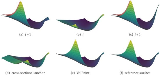
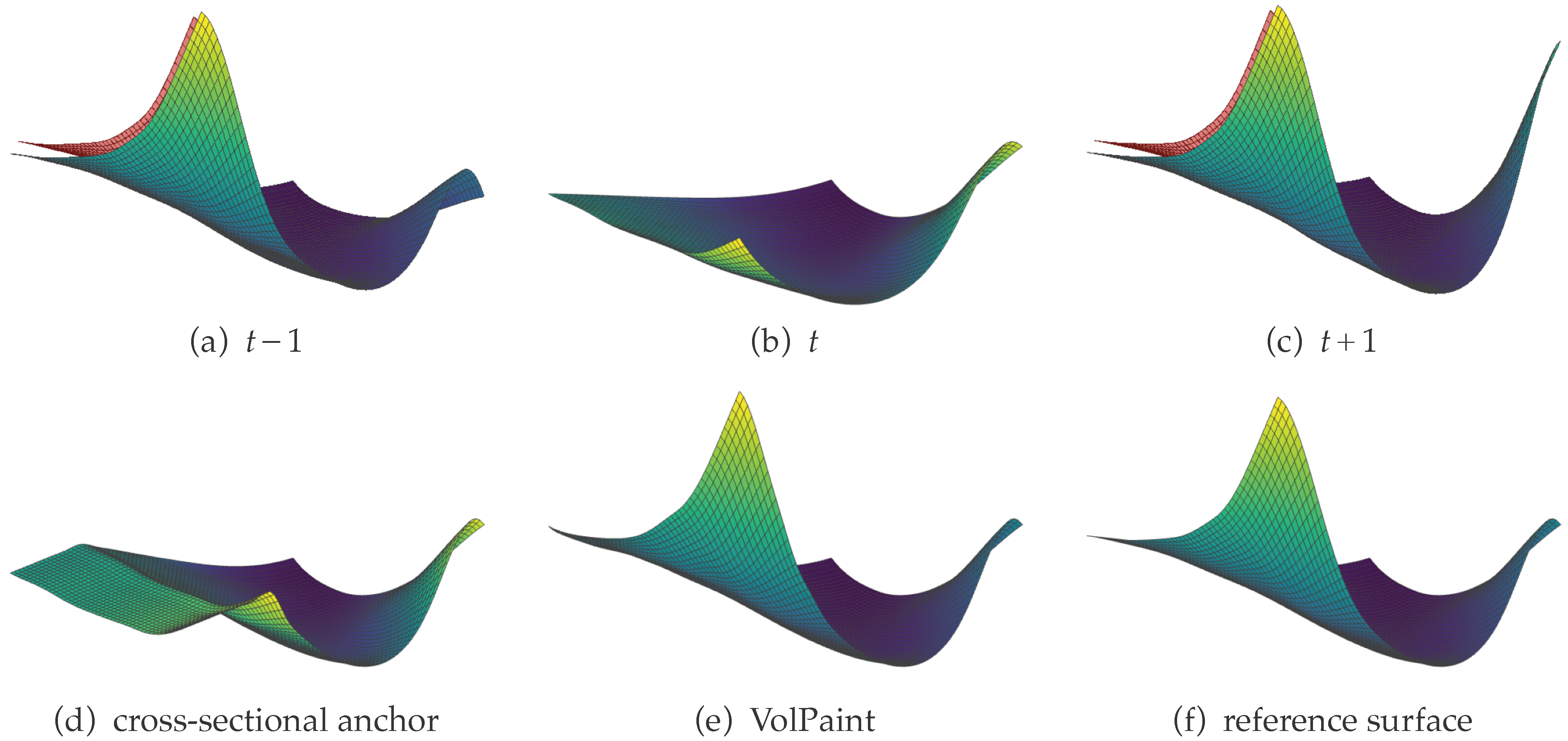
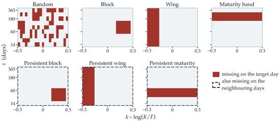
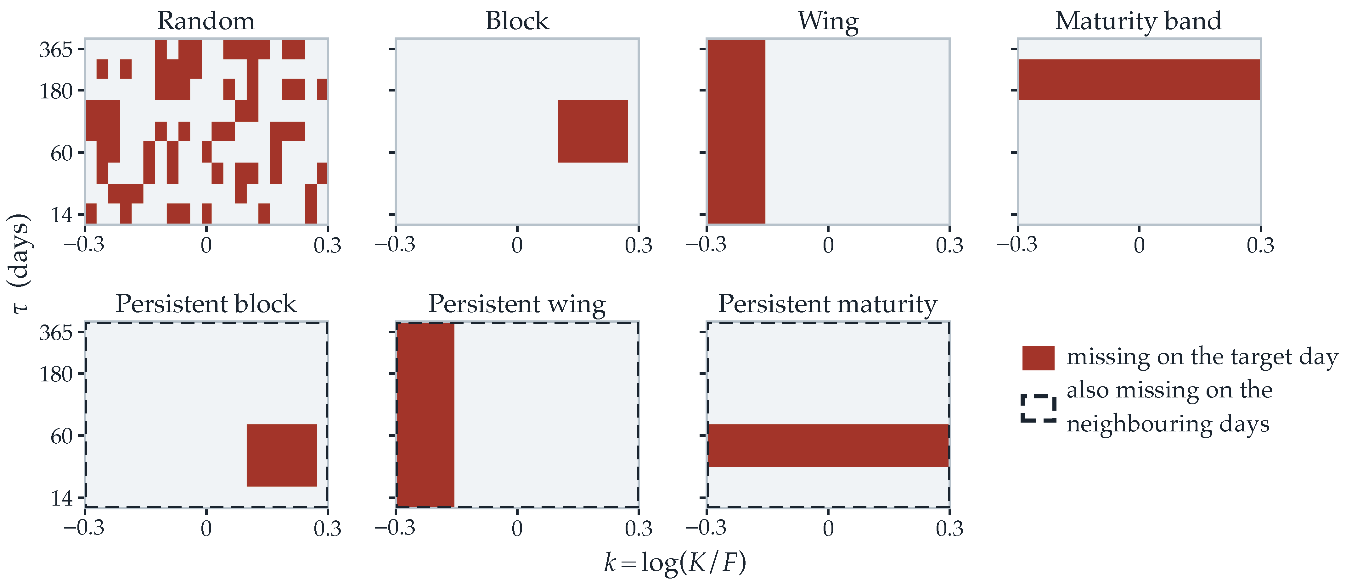
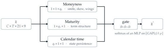
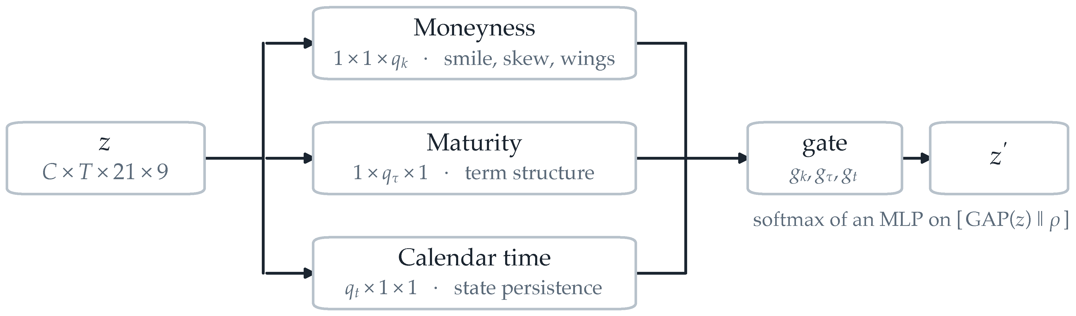
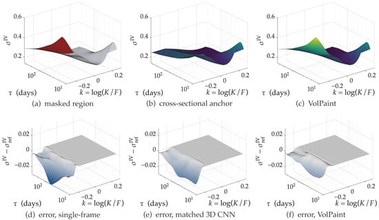
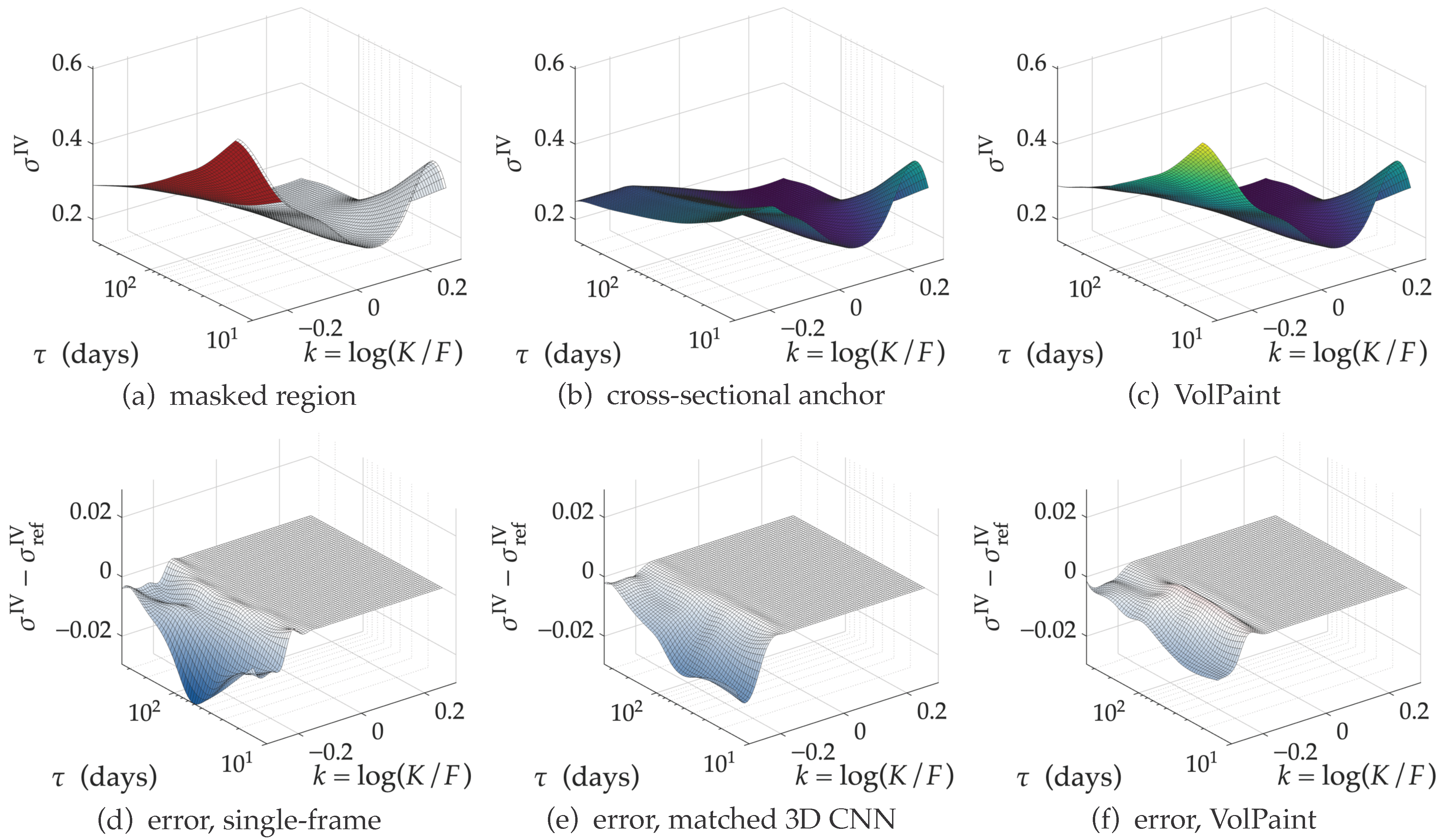
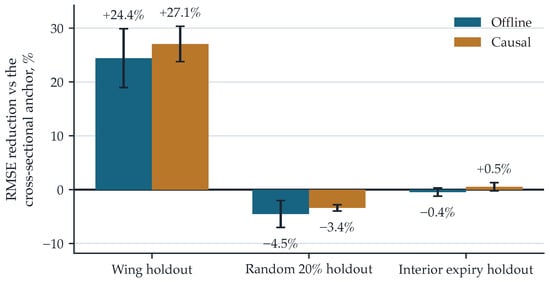
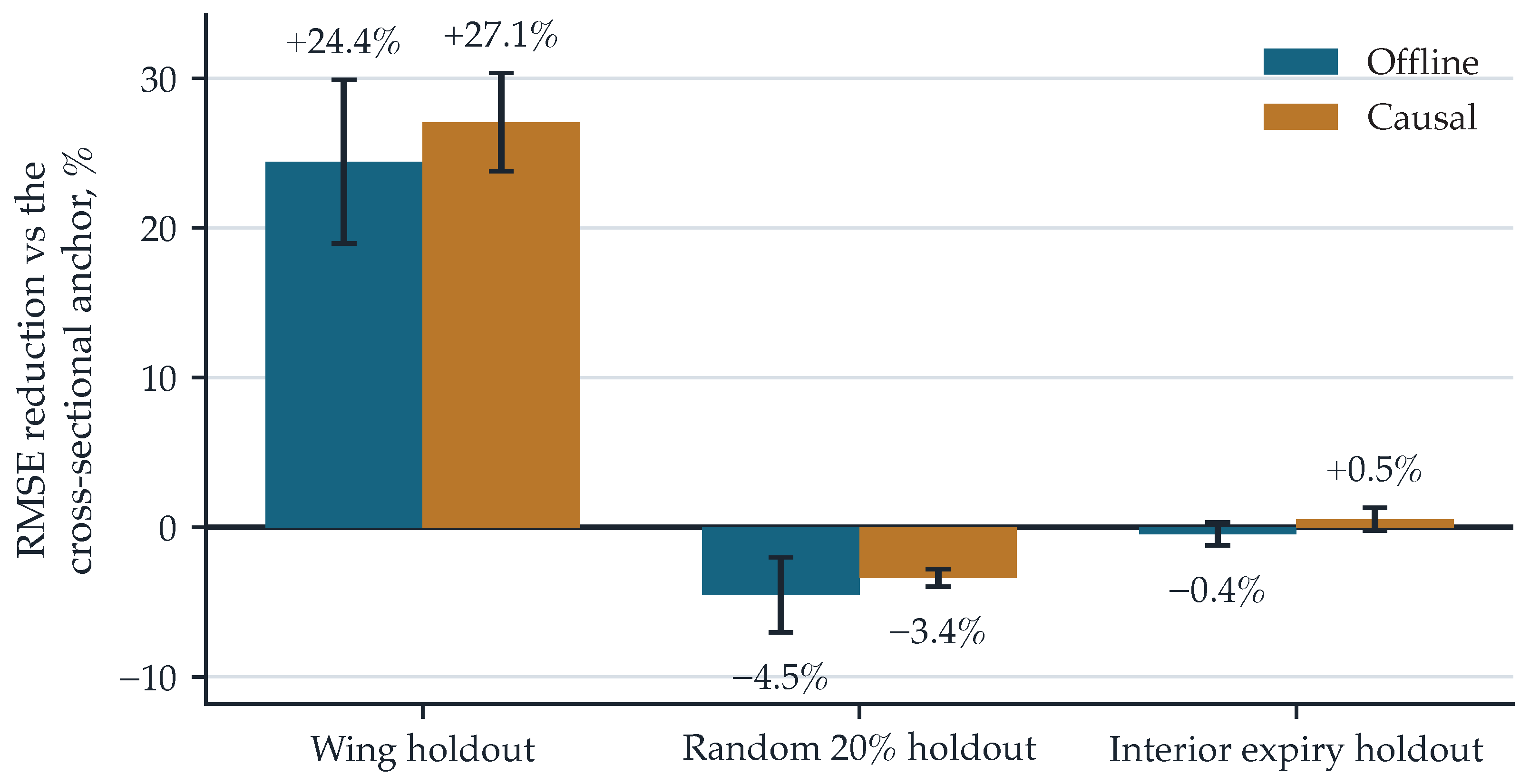
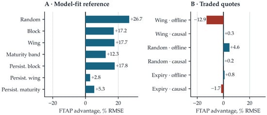
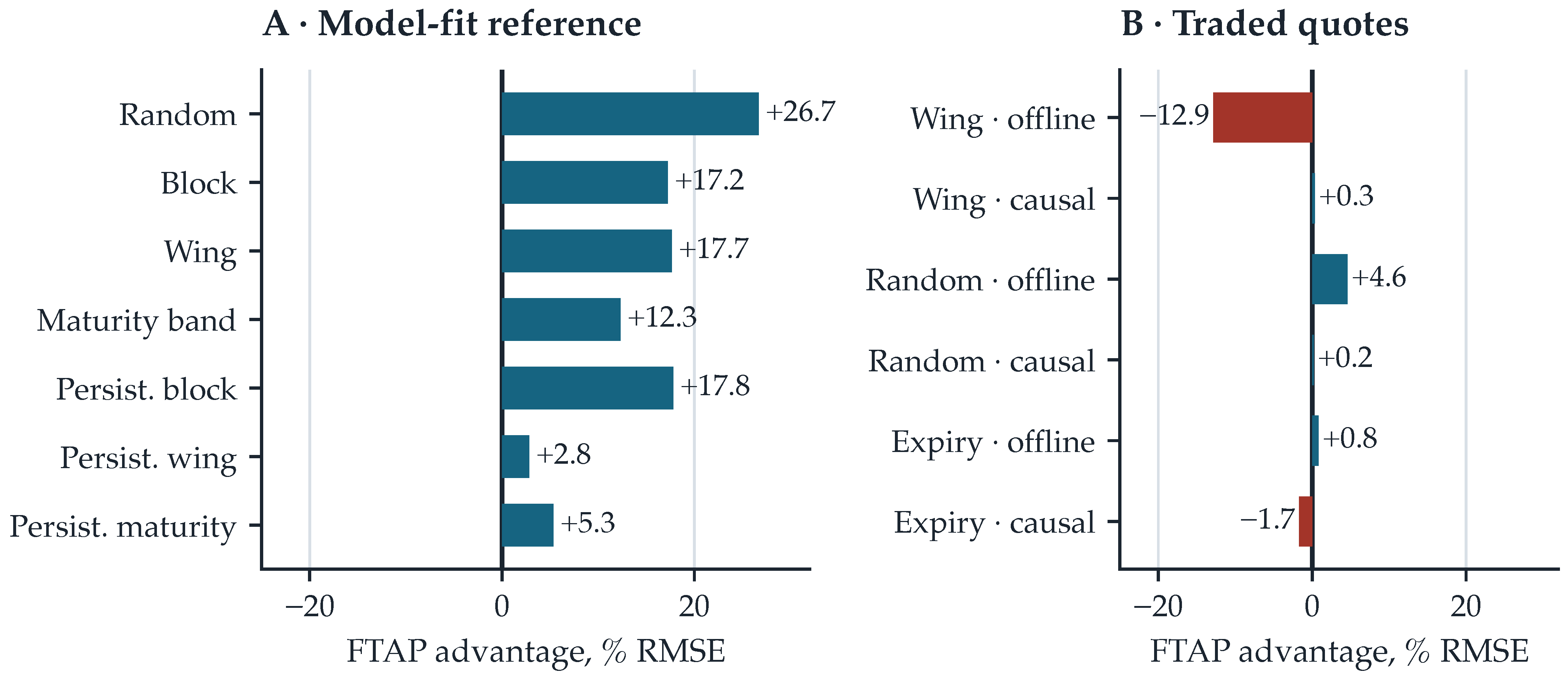

Disclaimer/Publisher’s Note: The statements, opinions and data contained in all publications are solely those of the individual author(s) and contributor(s) and not of MDPI and/or the editor(s). MDPI and/or the editor(s) disclaim responsibility for any injury to people or property resulting from any ideas, methods, instructions or products referred to in the content. |
© 2026 by the authors. Licensee MDPI, Basel, Switzerland. This article is an open access article distributed under the terms and conditions of the Creative Commons Attribution (CC BY) license.