Latitudinal and Elevational Shifts in South Korean Plant Occurrence Records: Sensitivity to Sampling Heterogeneity

Abstract

National occurrence databases combine sources with different objectives and spatiotemporal coverage, complicating the interpretation of changes in recorded locations. We evaluated the sensitivity of species-level shifts in mean recorded latitude and DEM-derived elevation to analytical specifications in an integrated South Korean vascular-plant database of 1,351,189 records, using 1980–2023 records for period-specific analyses. Empirical sensitivity comparisons were combined with controlled simulations of known centroid displacement. The primary analysis retained 1281 species and yielded across-species median shifts of +0.171° latitude and −102.7 m elevation. Aggregate estimates were similar before and after spatial thinning and record-count balancing. Positive latitude medians persisted under most specifications, but not under every spatial-support definition. Elevation estimates were more sensitive to temporal weighting and source composition: annual equal weighting reduced the median shift to −17.1 m, and omitting National Park records reversed its sign. In simulations, subtracting an assemblage-derived footprint markedly reduced recovery of imposed displacement. The empirical analyses characterize directional occurrence-centroid patterns and their sensitivity, rather than establish biological movement. Footprint subtraction cannot be assumed to recover unbiased change, and consistency across specifications does not demonstrate the absence of residual sampling bias.

1. Introduction

Distribution centers, range boundaries, and area occupied describe different aspects of spatial change [1]. Here, we examine shifts in recorded occurrence centroids, whose relationship to biological distributional change depends on the observation process. National occurrence databases provide broad spatial and temporal records for examining changes in recorded locations, but changes in their sampling geography can affect the resulting temporal patterns [2]. Recorded locations reflect both where organisms occur and where, when, and how observations are made [3,4,5]. An observed shift in mean recorded position describes a change in the retained occurrence records; it does not by itself distinguish biological distributional change from changes in observation geography.

Distinguishing changes in recorded occurrence centroids from biological distributional change is particularly important when national databases combine sources with different spatial and temporal coverage. The underlying survey programs may target different habitats, protected areas, taxonomic groups, or administrative objectives; begin and end in different years; and change field coverage or recording intensity through time. Spatial and temporal bias is widespread in occurrence databases and digitized collections [6,7,8,9], and geographic sample selection can affect presence-only inference [10]. Even if a species’ biological distribution does not change between periods, changes in observation locations or in the mixture of source datasets can alter the mean location of its records. This conditional example does not assume that species distributions are generally static or confined to a single point. Spatial thinning [11] and rarefaction [12] address particular record imbalances, whereas early–late comparability of geographic coverage requires separate evaluation [13,14].

Species-level changes in mean recorded latitude and mean DEM-derived elevation are evaluated as separate summary statistics, not as biologically equivalent responses. Latitude is read directly from occurrence coordinates, whereas elevation is derived from terrain at those coordinates and can vary sharply over short distances. Coordinate error, rounding, and mismatch between occurrence precision and environmental grain can affect the assigned elevation [15,16]. Source datasets that increasingly represent lowlands, mountains, wetlands, or protected areas can therefore alter an aggregate elevational signal without an equivalent change in latitude.

The empirical question is which observed centroid patterns persist when temporal weighting, source composition, and the set of comparison cells are changed. Here, spatial support means the set of cells meeting specified observation criteria. Restrictions on that support may change both the retained records and the target of estimation. Explicit observation-process models offer a complementary approach when structured effort data are available [17,18,19].

An assemblage-derived footprint summarizes locations observed across species within a source-year and is not an independent measurement of survey effort. Subtracting that footprint from recorded latitude or elevation may remove sampling displacement together with biological change shared among species. Controlled simulations with known center displacement allow us to test how much of that specified change is preserved. The empirical and simulation analyses therefore address the basis and limits of biological interpretation, without treating preprocessing or data volume as a guarantee of unbiased inference.

The South Korean record spans 1980–2023, combines five source datasets, and covers substantial geographic variation within a compact region. Earlier Korean plant studies addressed elevational distributions and climate-related habitat suitability for selected taxa [20,21,22], but they did not evaluate the dependence of occurrence-centroid estimates on temporal weighting, source composition, and spatial coverage in a national multi-source database. The database examined here was assembled under the national survey-data integration and standardization framework described by Lee and Hong [23]. We asked three methodological questions: (1) to what extent do species-level Late-minus-Early differences in mean latitude and mean elevation, and their across-species medians, retain their signs and magnitudes when temporal weighting, source composition, and the set of comparison cells are changed; (2) how do temporal changes in source representation and in source-year summaries of observed latitude and elevation relate to the sensitivity of those centroid-shift estimates; and (3) to what extent does subtracting an occurrence-derived assemblage footprint preserve a known common centroid displacement imposed under controlled simulations? We evaluate the sensitivity of occurrence-centroid estimates, rather than partitioning the empirical shifts into biological and sampling components. Known common displacement refers to the shared center shift specified in a simulation scenario, not to an established movement of the plants in the empirical database.

2. Materials and Methods

2.1. Study Data and Preprocessing

We analyzed 1,351,189 vascular-plant occurrence records from five national survey and specimen sources. Five source-dataset categories were distinguished by datasetName: the Survey of Baekdudaegan Protected Areas and the National Survey for Ecosystems in Korea (National Institute of Ecology), the Natural Resource Survey of National Parks (Korea National Park Service), the Survey of Inland Wetlands (National Institute of Ecology), and specimen records aggregated from the National Institute of Biological Resources (NIBR) and the National Science Museum. The first four categories represented survey programs, whereas Specimen Records was an analytical grouping of institutional repository records. We use the shortened labels Protected Areas, National Ecosystem, National Park, Inland Wetland, and Specimen Records. The provenance and integration of the underlying national survey and specimen datasets were documented previously [23,24], including the contributing programs and institutions and standardization based on common information on species identity, occurrence location, and survey time. We used all five source-dataset categories represented in the integrated plant database; no source-dataset category was selectively excluded from the primary analysis. The database is not an exhaustive inventory of all South Korean occurrence records available through public portals. The sources differed in mandate and geographic coverage: ecosystem surveys covered the country outside national parks, park surveys targeted national parks, wetland surveys targeted inland wetlands, the Protected Areas source represented the Baekdudaegan protected-area survey, and specimen repositories provided the longest historical coverage [23]. Species name, occurrence location, and survey time were the common elements available across sources [23]. Because abundance was not measured consistently, records were analyzed as presence-only occurrences. Records of legally designated endangered species were withheld during data integration to avoid disclosing conservation-sensitive locality information.

Records were integrated following Lee and Hong [23], including taxonomic name standardization against the National Species List of Korea [25], duplicate removal, and exclusion of records with missing or invalid coordinates. Coordinates were standardized to WGS84 (EPSG:4326). The integrated dataset contained 3473 species-level analytical units distinguished by standardized names—hereafter, “species” in the empirical analyses refers to these units.

Elevation was assigned to occurrence coordinates using the 30 m Digital Elevation Model of the Republic of Korea distributed by the National Geographic Information Institute (reference year 2024), resampled to a 1 km analytical grid [26]. The same elevation-assignment procedure was applied to all source datasets, yielding terrain elevations of 0–1863 m.

2.2. Primary Analysis of Shifts in Mean Recorded Position

The primary periods were Early (1980–2004), Middle (2005–2014), and Late (2015–2023); 1489 records outside this range were excluded from period-specific analyses. Period length was evaluated separately using equal nine-year periods. Records were sorted deterministically and thinned to one occurrence per unique combination of species, year, and 0.01° latitude–longitude cell.

Species were eligible when every period contained at least five unique 0.01° cells and two distinct years. Eligibility was recomputed after each restriction. The primary full-support rarefaction analysis included 1281 eligible species. These thresholds were screening floors rather than guarantees of precise species-level centroids.

For Raw and Thinned estimates, a species-period position was the arithmetic mean latitude or DEM-derived elevation of retained occurrences; its shift was the Late mean minus the Early mean. For occurrence rarefaction, each species was sampled without replacement to the same number of records in all three periods, using its smallest retained period-specific record count. This procedure was repeated 100 times. Each replicate shift was the sampled Late arithmetic mean minus the sampled Early arithmetic mean. The species-level rarefied point estimate was the median of the 100 replicate shifts. Positive latitude and elevation shifts indicate northward and upslope changes in mean recorded position, respectively. Overall point estimates were medians across species, limiting the influence of a few extreme species-level shifts. Percentile 95% intervals for this median were obtained from 5000 species-bootstrap resamples. Northward and upslope proportions were reported as descriptive summaries.

2.3. Sampling Heterogeneity and Estimator Sensitivity Analyses

We described sampling heterogeneity by source dataset and year using occurrence counts, sampled 0.01° cells, latitude and elevation ranges, and cell-weighted footprints. Source turnover denotes changes in whether sources are represented and in their shares of period-specific records. Footprint trajectories denote temporal changes in source-year summaries of observed locations. Latitude footprints equally weighted sampled-cell center latitudes; elevation was averaged within cells and then across cells. A source-dataset-year was footprint-valid when thinned records occupied at least five distinct 0.01° cells. Early-to-Late footprint changes were summarized by resampling valid source-dataset-years within periods. We also calculated each source dataset’s period-specific shares of occurrences, sampled-cell instances, and occurrences belonging to species eligible in the pooled analysis. These measures describe database composition and observation geography, not independently measured effort or detection probability.

For source-specific analyses, eligibility was recalculated within each source and aggregate shifts were reported only when at least 20 species met the criteria. Leave-one-source-dataset-out analyses omitted each source in turn, recomputed eligibility, retained species shared with the primary set, and repeated thinning and occurrence rarefaction. A reference consistent-source analysis retained sources with at least two sampled years and five unique 0.01° cells in both Early and Late. A stricter analysis retained sources with at least two footprint-valid years in both Early and Late. Aggregate sign reversal required an actual change in the sign of the across-species median, and species-level reversal required opposite non-zero signs for the same species.

For repeated spatial support, thinned records were assigned to 0.05°, 0.1°, and 0.2° grids. Cells were retained under three alternative Early-and-Late criteria: at least two sampled years per period, at least three years per period, or at least 20 thinned occurrences per period. The 0.1°/two-year rule was specified before its output was inspected and served as the reference repeated 0.1° common spatial support. All nine combinations were reported, with eligibility and occurrence rarefaction recalculated within each mask. This analysis differs from the footprint-paired comparison, which used footprint-valid records without the repeated 0.1° mask.

Temporal sensitivity was evaluated using equal nine-year periods (1997–2005, 2006–2014, and 2015–2023) and by giving sampled years equal weight. The equal-period comparison changes both period duration and the calendar years included; it is therefore not a test of smoothing strength over an identical observation window.

For annual weighting, mean latitude and elevation were first calculated for each species in each year from thinned records and then averaged across years within each period. An auxiliary year-rarefaction estimator sampled the same number of distinct years from every period for each species in 100 replicates and used the median replicate shift as the species estimate. Eligibility, rarefaction, and bootstrap settings otherwise matched the primary analysis.

A combined sensitivity analysis applied equal nine-year periods, the three strict consistent sources, the reference repeated 0.1° spatial mask, standard eligibility, and equal weighting of annual centroids. A 100-replicate year-rarefaction version was also calculated. This combined design was specified before its output was inspected and was not treated as a replacement for the primary estimate.

Sensitivity was evaluated relative to full-support occurrence rarefaction, using species eligible in both specifications for paired comparisons. We reported the median within-species difference, its percentile 95% interval from 5000 paired species-bootstrap resamples, Spearman correlation, sign agreement, and strict sign reversal. Aggregate persistence refers to retention of the sign of the across-species median; magnitude changes and species-level agreement are separate summaries. These comparisons describe sensitivity under specified restrictions, not a universal threshold of acceptable bias or a test certifying accurate biological inference.

2.4. Diagnostic Footprint Residualization

We compared residualized and uncentered shifts using only footprint-valid source-years, defined as those with thinned records in at least five distinct 0.01° cells (Section 2.3). Here, p indexes source datasets, y indexes survey years, s indexes species, t indexes periods, b indexes rarefaction replicates, and i indexes occurrence records. Latitude and elevation were processed separately, with z denoting the coordinate or terrain value for the axis under analysis.

For source p and year y, the latitude footprint is the equally weighted mean of the latitudes of observed cell centers. For elevation, values are first averaged within each observed cell and then equally averaged across cells. We denote the resulting source-year footprint by F_p,y(z). It is a summary of the occurrence assemblage, not an independent estimate of survey effort.

Within each species, period, and replicate, exactly the same occurrence records were selected for the uncentered and residualized calculations. For each selected record, the residualized value is z^∗(i) = z(i) − F_p(i),y(i)(z). Let Δ(s, b) be the uncentered Late-minus-Early difference in means, and let F_mean(s, t, b) be the mean footprint associated with the records actually selected for species s in period t and replicate b. The paired replicate-level identity is:

Δ^∗(s, b) = Δ(s, b) − [F_mean(s, Late, b) − F_mean(s, Early, b)].

The species-level point estimate is the median of its replicate shifts. In general, taking medians does not convert this replicate-level identity into a difference between independently calculated medians. The reference is matched uncentered rarefaction on the same footprint-valid records, not the full-support estimate or the repeated 0.1° common-support analysis.

2.5. Simulation Design and Evaluation

The simulations tested the recovery of a specified center displacement, not whether centroid displacement represents all forms of range change. Each replicate used an 81 × 81-cell virtual landscape, combining latitude from 32.0° to 40.0° at 0.1° intervals and elevation from 0 to 3200 m at 40 m intervals, rather than a Korean DEM. It generated 1400 bivariate Gaussian species profiles, with baseline latitude drawn from 34° to 38°, baseline elevation from 800 to 2200 m, latitude standard deviation from 0.25° to 0.60°, and elevation standard deviation from 120 to 300 m. The 3 × 3 truth matrix crossed latitude shifts of −0.3°, 0°, and +0.3° with elevation shifts of −100 m, 0, and +100 m. These profiles and imposed shifts define a controlled estimator test rather than a mechanistic model of plant distributions.

Three virtual programs had baseline sampling centroids of 34.5°/900 m, 36.2°/1500 m, and 38.1°/2100 m, with latitude and elevation standard deviations of 1.35° and 700 m. Each period contained two survey years. D is the standardized distance from the corresponding program-year sampling centroid: the square root of the sum of squared latitude and elevation differences, each divided by its axis-specific standard deviation before squaring. Sampling intensity I was I_p,y(x) = exp(−0.5D²) for D² ≤ 9 and zero otherwise. Under stable sampling, program centroids and widths did not change. Under empirically scaled shifting sampling, every centroid moved +0.396° latitude and −235.7 m elevation from Early to Late, with half that displacement in the Middle, and width multipliers were 1.00, 0.85, and 0.70. These displacement magnitudes approximated the empirical across-source-dataset 75th percentile of absolute footprint changes. Here, “stable sampling” denotes fixed analytical sampling-intensity surfaces; the occurrence-derived assemblage footprint was re-estimated from realized records and could therefore still track biological redistribution imposed across species.

Biological suitability G and sampling intensity I were constructed independently. Conditional observed-cell probability was

$$\mathrm{P}(X=x|s,p,y)={\displaystyle \frac{G_{s,t}\left(x\right)I_{p,y}\left(x\right)}{{\sum }_x{G}_{s,t}\left(x\right)I_{p,y}\left(x\right)}}.$$

Detected events were drawn from Binomial(E_t, 0.85), with intended events per program-year of 6, 10, and 16 in Early, Middle, and Late. Cells were sampled with replacement. Each selected cell generated 1 + Poisson[1.5I_p,y(x)] records so that deterministic thinning could be evaluated.

The empirical eligibility rule was applied to each design. Of 1400 jointly eligible species, a fixed set of 1000 was evaluated independently of simulated outcomes. Estimators were raw, thinned, rarefied, footprint-residualized, simulation common-support, and known sampling-intensity-weighted. The last estimator used known sampling intensity, which is unavailable for these empirical data, and served only as a benchmark. Simulation common support was the intersection of positive-intensity masks, distinct from the empirical repeated-grid restriction. Thirty simulation replicates were completed for each of the 18 scenarios formed by two sampling geographies and nine truth combinations.

Root-mean-square error (RMSE) summarized the species-level difference between estimated and known shifts: $\mathrm{RMSE}=\sqrt{\mathrm{mean}\left[{\left({\mathit{estimated}}_i-{\mathit{known}}_i\right)}^2\right]}$. Truth-recovery slope was the ordinary least-squares slope of estimated on known shift across the 3 × 3 truth matrix. Sign recovery was the percentage of estimates with the correct sign among non-zero truth values. The axis-specific threshold-exceedance rate in the joint-null scenario was calculated separately for each axis among species for which both known shifts were zero: 100 mean(|estimated latitude shift| > 0.05°) for latitude and 100 mean(|estimated elevation shift| > 25 m) for elevation. This is a threshold-exceedance measure, not a hypothesis-test error rate. Detection probability and redistribution thresholds were fixed simulation settings, not estimated from the empirical plant data.

Performance was summarized across replicates using medians and 2.5th–97.5th simulation quantiles. We also calculated within-replicate slope differences and percentage attenuation relative to Rarefied estimates. Simulation quantiles describe variation among simulation replicates and are distinct from empirical species-bootstrap intervals. All analyses and figures were produced in Python (v.3.11).

3. Results

3.1. Data Coverage and Primary Shifts in Mean Recorded Position

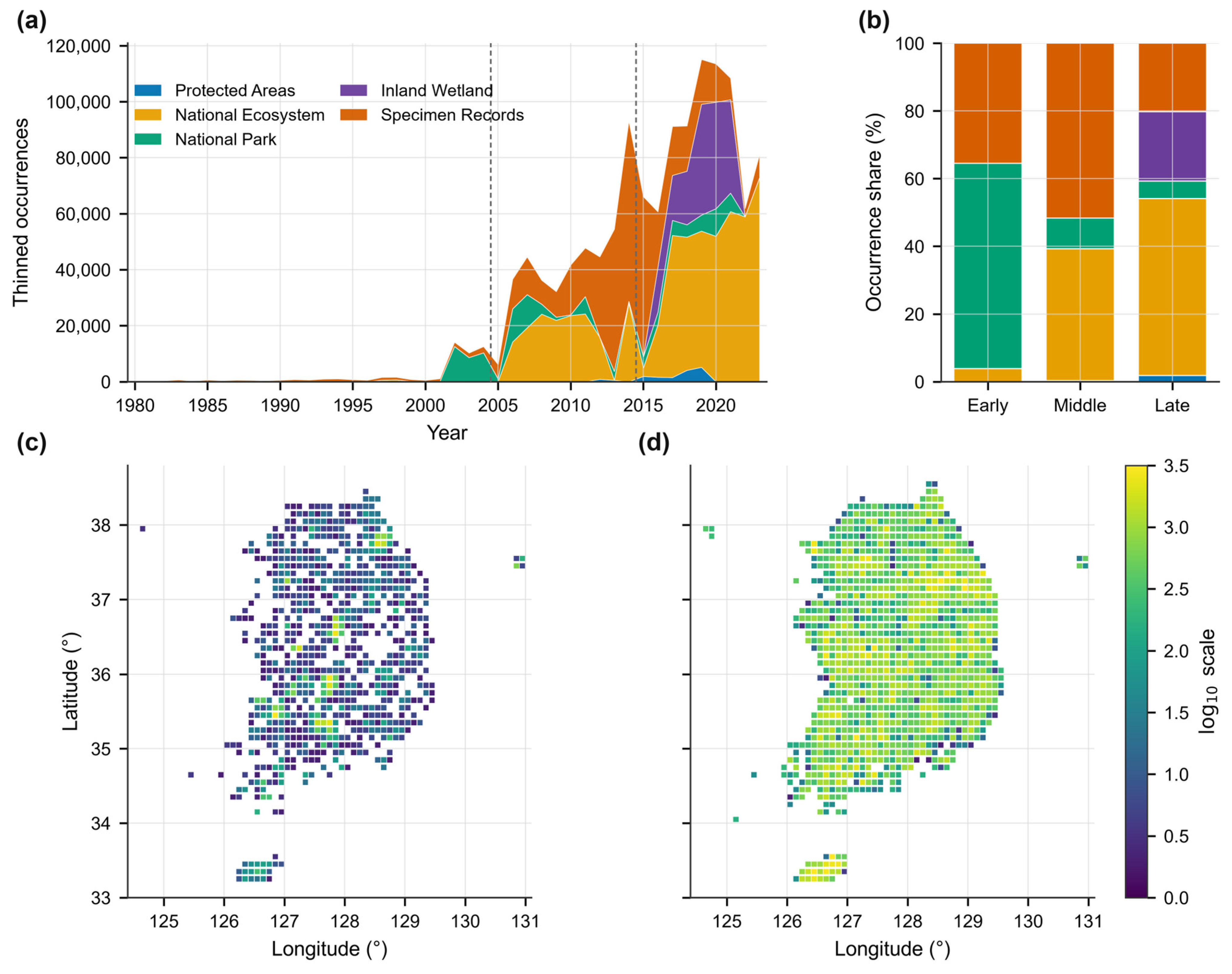
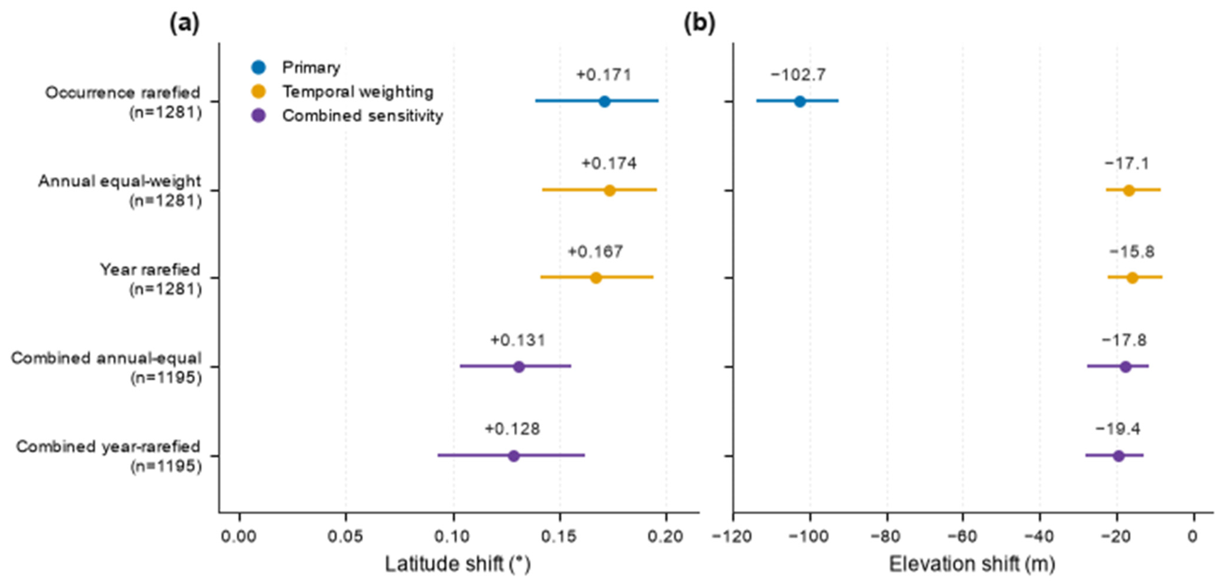
The integrated analysis dataset contained 1,351,189 records representing 3473 vascular-plant species-level analytical units. Coverage increased from 53,572 Early records to 833,267 Late records, with large changes in source-dataset and spatial composition (Table 1; Figure 1). The primary full-support occurrence-rarefaction design retained 1281 eligible species. Its across-species median was +0.171° latitude (species-bootstrap percentile 95% interval +0.139 to +0.197), with 65.1% of species northward, and −102.7 m elevation (−113.5 to −92.4; Figure 2), with 23.0% upslope.

Table 1. Data coverage and sample sizes through the empirical analysis.

Analysis Step	Years/Design	Retained Occurrences	Sampled Cells/Grids	Species-Level Analytical Units	Note
Integrated analysis dataset	All available	1,351,189	30,267 0.01° cells	3473	1489 records outside 1980–2023
Early support	1980–2004	51,529 thinned	2754 0.01° cells	—	53,572 unthinned records
Middle support	2005–2014	437,494 thinned	19,311 0.01° cells	—	462,861 unthinned records
Late support	2015–2023	789,521 thinned	23,570 0.01° cells	—	833,267 unthinned records
Full-support rarefaction	Primary periods	—	—	1281	100 occurrence-rarefaction replicates
Repeated 0.1° common spatial support	≥2 years in Early and Late	691,128	446 coarse grids	1239	Eligibility recomputed
Combined: equal-period years	1997–2023	1,340,657	—	—	Three nine-year periods
Combined: strict source datasets	Three source datasets	1,153,936	—	—	National Ecosystem, National Park, Specimen
Combined: 0.01° thinning	Equal periods and strict sources	1,092,930	—	—	Deterministic
Combined: repeated support	0.1°, ≥2 years in Early and Late	573,513	403 coarse grids	—	Pooled strict-source support
Combined eligible records	Annual-equal estimator	502,857	403 coarse grids	1195	1149 shared with primary

Species-level analytical units denote all standardized names in the integrated-dataset row and eligible species wherever counts are reported in subsequent rows. The combined-analysis restrictions are cumulative, from equal-period years through eligible-record selection.

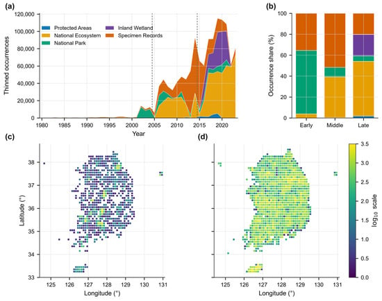
Figure 1. Temporal, geographic, and source-dataset composition of the plant occurrence data. (a) Annual numbers of deterministically thinned occurrences by source dataset; dashed lines delimit Early (1980–2004), Middle (2005–2014), and Late (2015–2023). (b) Source-dataset shares of all integrated occurrences in each period. (c) Early and (d) Late horizontal geographic coverage in 0.1° cells. In (c,d), color indicates log10(n + 1), where n is the number of thinned occurrences per cell; values above 3.5 use the uppermost color. Maps describe occurrence coverage rather than standardized survey effort.

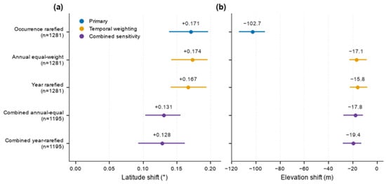
Figure 2. Latitudinal and elevational estimates under temporal weighting and the combined sensitivity analysis. (a) Latitudinal shifts (°) and (b) elevational shifts (m), calculated as Late minus Early. Points are across-species medians; bars are percentile 95% intervals from 5000 species-bootstrap resamples. Latitude changed comparatively little after annual equal weighting and year rarefaction, whereas the negative elevational magnitude was greatly attenuated. Combined estimates additionally restrict periods, source datasets, and repeated 0.1° common spatial support.

Raw and deterministic-thinning estimates were similar to full-support rarefaction. Raw shifts were +0.174° (+0.138 to +0.201) and −99.5 m (−108.7 to −88.5); thinned shifts were +0.172° (+0.142 to +0.195) and −102.8 m (−111.6 to −92.0). Balancing occurrence counts among periods therefore changed these pooled estimates little, although it did not address temporal or source-dataset composition. Thus, the aggregate directions were already present in the Raw comparison and were not newly introduced by thinning or occurrence rarefaction. This similarity does not establish the absence of sampling effects shared by the compared record sets.

3.2. Source Composition and Temporal Sensitivity

National Ecosystem records increased from 3.8% of Early occurrences to 52.3% of Late occurrences, whereas National Park records declined from 60.6% to 5.1%. Protected Areas contributed 0.04% in Early and 1.8% in Late. Inland Wetland had no Early records and contributed 20.5% in Late; Specimen Records declined from 35.5% to 20.2%. The source datasets dominating the integrated database therefore differed sharply between boundary periods (Figure 1).

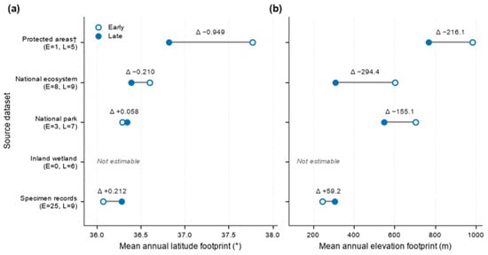
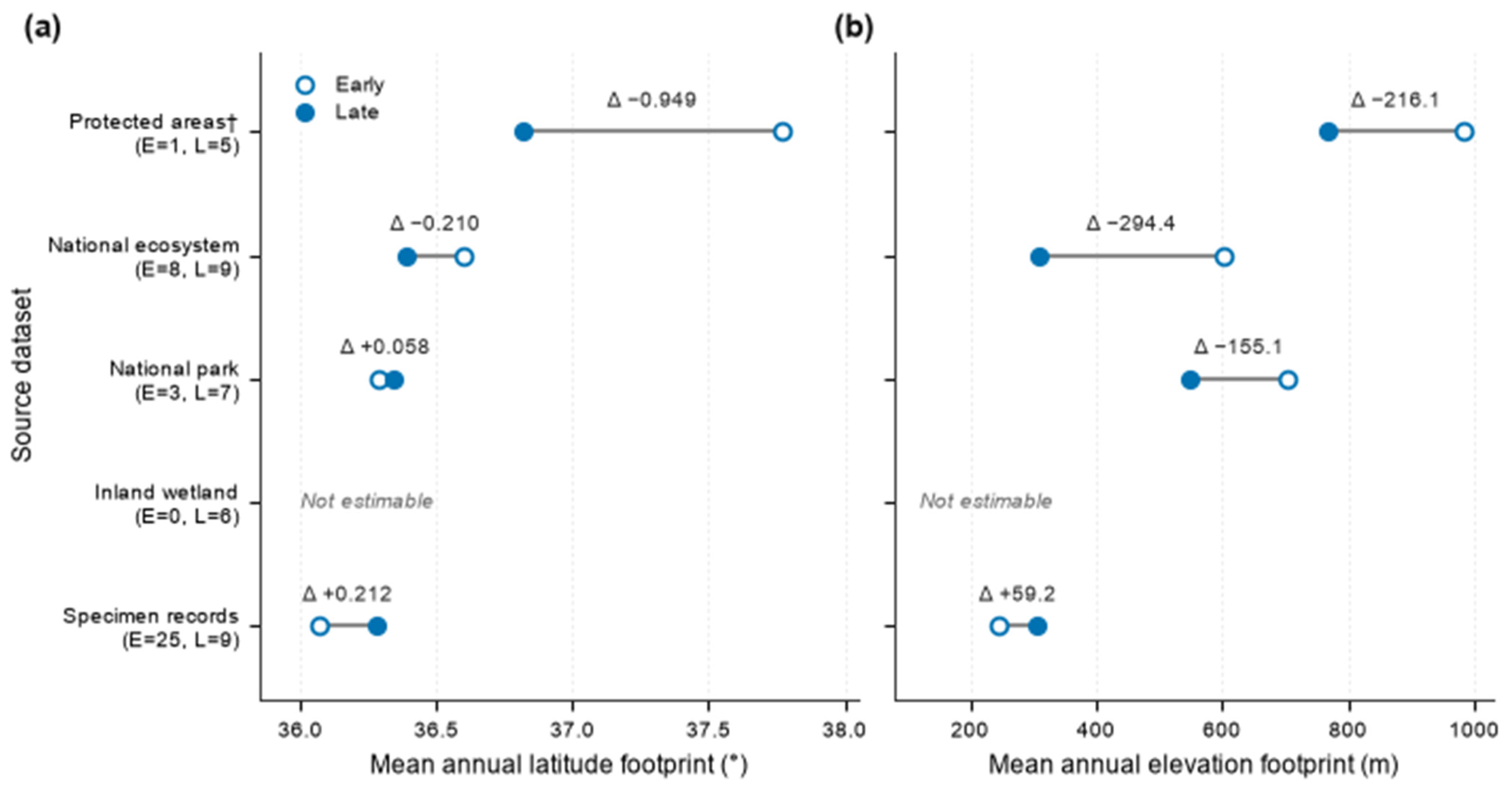
Among source datasets with at least three footprint-valid years in each boundary period, the Specimen Records footprint shifted northward by +0.212° (source-dataset-year bootstrap 95% interval +0.049 to +0.352) and upward by +59.2 m (+38.5 to +80.2). The National Ecosystem footprint shifted downward by −294.4 m (−362.3 to −224.0). The National Park footprint changed by +0.058° (−0.744 to +0.741) and −155.1 m (−309.3 to −37.4). Protected Areas had the largest absolute latitude change, −0.949°, but its Early estimate used only one footprint-valid year and was not interpreted as a stable trajectory (Figure 3).

Figure 3. Early and Late latitude and elevation sampling footprints by source dataset. (a) Latitude (°) and (b) elevation (m) sampling footprints. Source datasets are defined by the datasetName field in the integrated occurrence data. Open and filled circles are the means of footprint-valid annual footprints in the Early and Late periods, respectively; connecting segments show their direction and magnitude of change, and labels give Late-minus-Early differences. Parentheses give the numbers of footprint-valid Early (E) and Late (L) years. The dagger marks Protected Areas, which had only one footprint-valid Early year and therefore limited temporal support; Inland Wetland was not estimable because it had no Early records. The figure describes sampling geography rather than species redistribution.

Using three equal nine-year periods retained 1282 species and yielded +0.182° (species-bootstrap percentile 95% interval +0.155 to +0.213) and −109.9 m (−122.3 to −100.8). Among 1211 species shared with the primary analysis, Spearman correlations were 0.905 for latitude and 0.945 for elevation; paired median differences were +0.009° (+0.002 to +0.015) and −6.7 m (−8.6 to −4.6).

Equal weighting of annual centroids retained all 1281 primary species and produced +0.174° (+0.142 to +0.195) but only −17.1 m (−22.9 to −8.4). Year rarefaction gave +0.167° (+0.141 to +0.195) and −15.8 m (−22.4 to −7.7). Relative to full-support occurrence rarefaction, the year-rarefied paired differences were +0.006° (−0.009 to +0.025) and +83.7 m (+77.7 to +90.8). Species-level correlations were 0.837 and 0.769, and strict sign reversals occurred for 15.4% and 24.5% of species. Both annual-equal and year-rarefied estimates had 44.7% upslope; the year-rarefied northward proportion was 67.4%, compared with 65.1% under full-support occurrence rarefaction. Thus, temporal weighting had little effect on the aggregate latitudinal direction but greatly attenuated the negative elevational magnitude (Figure 2).

Thinned records were temporally concentrated: 2002 supplied 28.0% of Early records and 2014 supplied 21.5% of Middle records. A single year contributed more than half of the records in 19.9% of Early and 32.7% of Middle species-period cases. These concentrations explain why annual weighting was a necessary sensitivity analysis rather than a cosmetic re-expression of occurrence rarefaction.

3.3. Source and Spatial Support Sensitivity

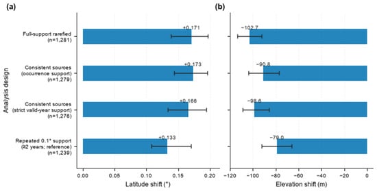
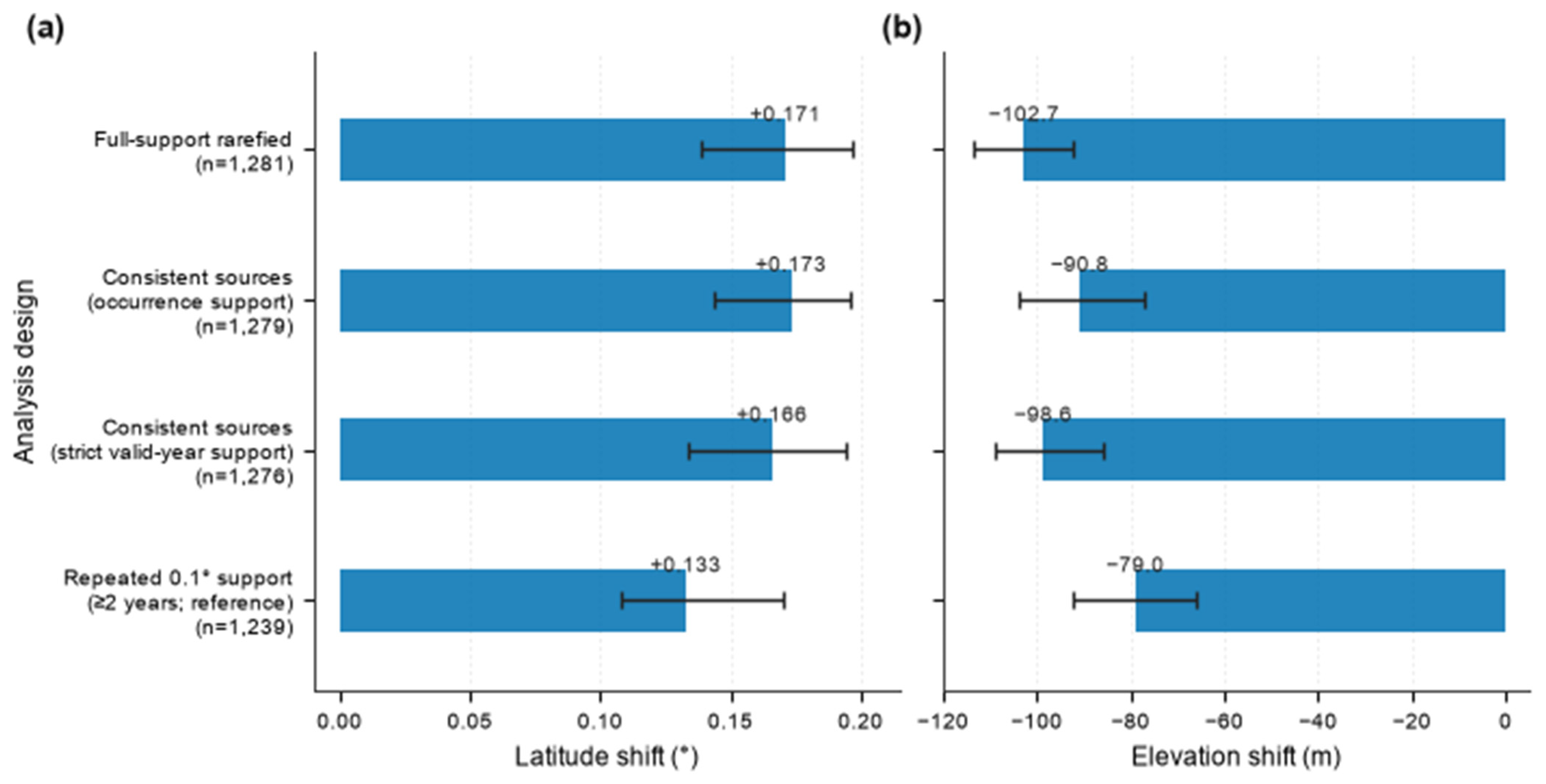
The occurrence-support consistent-source analysis retained four source datasets and 1279 species, yielding +0.173° (+0.144 to +0.196) and −90.8 m (−103.9 to −77.2). Requiring at least two footprint-valid years in both Early and Late retained National Ecosystem, National Park, and Specimen Records, with 1276 eligible species, and yielded +0.166° (+0.134 to +0.194) and −98.6 m (−108.8 to −85.6).

The reference repeated 0.1° common spatial support retained 446 cells and 1239 eligible species. Median shifts were +0.133° (+0.108 to +0.170) and −79.0 m (−92.1 to −65.9), with 60.6% northward and 29.6% upslope (Figure 4). Across all nine support combinations, eight latitude medians were positive and all nine elevation medians were negative. The 0.05°/minimum-20-occurrence criterion produced a negative latitude median, and the 0.1°/minimum-20-occurrence interval included zero; the northward result was therefore not invariant to every support definition (Table A1).

Figure 4. Shifts in mean recorded latitude and elevation under temporally consistent source datasets and repeated 0.1° common spatial support. (a) Latitudinal shifts (°) and (b) elevational shifts (m), calculated as Late minus Early. Bars are across-species medians; whiskers are percentile 95% intervals from 5000 species-bootstrap resamples. Full-support rarefaction is shown for comparison. The 0.1°/at-least-two-years criterion is the reference repeated spatial support; all nine specifications are in Table A1.

Every leave-one-source-dataset-out latitude median was positive, ranging from +0.112° after excluding Specimen Records to +0.285° after excluding National Park. Elevation behaved differently: excluding National Park changed the aggregate median from −102.7 m to +29.1 m and was the only aggregate sign reversal. Excluding Specimen Records yielded −243.2 m; the downslope direction remained but its magnitude increased substantially (Table A2).

The National Park omission retained 1055 common eligible species, of which 61.6% had positive elevation shifts. National Ecosystem omission retained 1218 species and produced −89.2 m, whereas Inland Wetland omission retained 1279 species and produced −93.6 m. No single source-dataset omission altered both axes in the same way. For these 1055 species, the corresponding full-support elevation median was −92.5 m versus +29.1 m after omission; species-level ρ was 0.467, and 432 species (40.9%) showed strict sign reversals.

Within-source eligibility reached the reporting threshold for three source datasets. National Ecosystem retained 87 species and yielded +0.012° (−0.085 to +0.089; 52.9% northward) and −92.2 m (−123.6 to −48.5; 20.7% upslope). National Park retained 662 species and yielded +0.233° (+0.193 to +0.282; 68.6%) and −79.2 m (−93.5 to −69.3; 27.0%). Specimen Records retained 934 species and yielded +0.276° (+0.237 to +0.302; 72.6%) and +52.8 m (+46.6 to +59.7; 72.7%). Protected Areas and Inland Wetland did not retain at least 20 eligible species and were not assigned aggregate within-source estimates.

The combined sensitivity retained 573,513 records within 403 repeatedly sampled 0.1° cells; 502,857 records represented 1195 eligible species, of which 1149 were shared with the primary set (Table 1). Equal weighting of annual centroids yielded +0.131° (+0.103 to +0.156), with 61.3% northward, and −17.8 m (−27.4 to −11.4), with 42.6% upslope. Auxiliary year rarefaction yielded +0.128° (+0.093 to +0.162) and −19.4 m (−28.1 to −12.8), with 60.8% northward and 42.5% upslope.

For the 1149 common species, combined annual-equal estimates differed from full-support rarefaction by −0.037° (−0.056 to −0.019) and +92.9 m (+86.5 to +100.8). Spearman correlations were 0.718 and 0.724; sign agreement was 78.4% and 74.2%, and strict reversals occurred for 21.6% and 25.8% of species. The simultaneous restrictions retained both aggregate directions but did not reproduce the primary magnitudes or species ordering.

3.4. Footprint Residualization and Simulation Performance

Paired footprint residualization yielded +0.022° (−0.003 to +0.040) and +67.1 m (+59.3 to +72.0). Its reference was matched uncentered rarefaction on footprint-valid records—not full-support rarefaction or repeated 0.1° common spatial support. For both axes, the paired median difference is the median of within-species differences and need not equal the difference between the two across-species medians. For elevation, residualized minus uncentered was +180.5 m (paired species-bootstrap percentile 95% interval +174.1 to +188.8), with ρ = 0.530, sign agreement 612/1281 (47.8%), strict reversal 669/1281 (52.2%), and median absolute change 181.8 m. For latitude, the corresponding values were −0.198° (−0.212 to −0.183), ρ = 0.895, 82.3% agreement, 227/1281 reversals (17.7%), and 0.225° median absolute change.

The known-truth simulations clarified why the empirical footprint-residualized estimates cannot be interpreted as bias-corrected redistribution. Under empirically scaled shifting sampling, median truth-recovery slopes were 0.712 for Rarefied latitude (2.5th–97.5th simulation quantiles 0.703–0.720) and 0.779 for Rarefied elevation (0.767–0.789), versus 0.233 (0.215–0.254) and 0.172 (0.149–0.199) after footprint residualization. Within-replicate slope differences (residualized minus Rarefied) had medians −0.479 and −0.607, corresponding to 67.3% and 77.8% additional attenuation; residualized slopes were lower in all 30 replicates on both axes (Table A3).

This loss of recovery was accompanied by larger error and poorer sign recovery. Under shifting sampling, median RMSE increased from 0.267° to 0.305° for latitude and from 83.3 to 110.7 m for elevation; median sign recovery declined from 80.4% to 58.9% and from 83.7% to 55.6%. The known-intensity-weighted benchmark, which used sampling information unavailable for the empirical data, had slopes of 0.747 for latitude and 0.841 for elevation under shifting sampling. Under stable sampling, Rarefied slopes were 0.881 (0.869–0.887) and 0.905 (0.896–0.916), residualized slopes were 0.179 (0.164–0.195) and 0.056 (0.034–0.074), and benchmark slopes were 0.936 and 0.974. Strong attenuation therefore also occurred when the analytic sampling geography was stable (Table A3). All 1400 generated species met the eligibility criteria in every scenario and replicate; performance comparisons used the same selected subset of 1000 species across all six estimators. The simulations therefore did not assess selection or failure near the eligibility thresholds.

4. Discussion

4.1. Interpretation and Sensitivity to Sampling Heterogeneity

The principal inferential result was a contrast between the two axes, not a claim about a shared plant response. The latitude median remained positive under the primary, equal-period, annual-weighted, consistent-source, leave-one-source-out, reference repeated-support, and combined sensitivity analyses. Exceptions under alternative spatial-support definitions and differences in magnitude remained. Within this integrated database, the evaluated designs nevertheless support a comparatively persistent apparent northward direction.

Elevational inference was more conditional. Its median remained negative after annual balancing and in the combined sensitivity, but annual equal weighting reduced the magnitude from approximately −103 m to −17 m, and omitting National Park records changed the aggregate estimate to +29.1 m. The apparent downslope magnitude, and under one source omission its direction, therefore depended strongly on temporal weighting and source-dataset composition. The apparent downslope direction contrasts with the upslope plant optimum reported by Lenoir et al. [27], but its sensitivity across designs precludes interpreting that contrast as evidence for a distinct biological driver. The elevational ranges reported by Shin et al. [20] for Baekdudaegan vascular plants provide a regional baseline, but describe elevational ranges rather than temporal changes in occurrence centroids and cannot be directly compared in direction or magnitude. These contrasts describe inference from this database rather than a biological difference between latitudinal and elevational plant responses. These analyses cannot separate the contributions of sampling design and biological redistribution to either signal. Persistence under the evaluated restrictions does not rule out residual sampling bias.

Changes in survey coverage and temporal sampling bias can affect spatial summaries [1,2]. Occurrence-weighted and annual-equal estimates differ in the influence assigned to heavily recorded years. The pronounced sensitivity of elevation to this choice shows that temporal weighting matters for interpretation; it does not establish that either weighting scheme recovers biological movement.

Changing source composition can alter the geographic locations represented in pooled records. The source-restricted comparisons show that elevational inference is sensitive to this composition, but they do not partition the independent effects of individual sources from biological change.

Leave-one-source-dataset-out analysis made the elevational sensitivity especially clear: removing National Park records reversed the aggregate sign, whereas removing Specimen Records strengthened the negative magnitude. Omitting Inland Wetland records still yielded a negative elevation median of −93.6 m, so the addition of late-period wetland records alone did not explain the downslope result. Because omissions also changed eligibility, aggregate estimates were accompanied by common-species comparisons. The National Park result is therefore consistent with changes in the relative contributions of the remaining sources and in the species and locations included in the analysis. It should not be interpreted as evidence that National Park records alone accounted for the downslope signal. The limited effect of the stricter source criterion indicates low sensitivity to this particular boundary case, rather than elimination of source-related sampling bias.

Repeated 0.1° common spatial support improves geographic overlap between periods but does not establish identical sites, effort, or within-cell sampling locations. It also restricts the regions and species represented. The persistence of positive latitude medians under most, but not all, support definitions therefore indicates conditional stability rather than removal of observation bias.

An occurrence-derived assemblage footprint is not an independent measure of survey effort. Subtraction can remove shared biological change together with sampling displacement. It produces a change relative to that footprint, rather than the uncentered change in mean recorded position. The matched comparison isolates the effect of subtraction on the same footprint-valid records, but cannot determine which component was removed; a positive residualized elevation estimate is therefore not evidence of biological upslope movement.

The known-truth experiment shows that footprint subtraction can attenuate an imposed shared displacement. This does not establish unbiasedness of rarefaction or a biological lower bound for the empirical estimates, because attenuation and residual sampling bias can coexist. Performance is conditional on the simulated profiles and sampling surfaces; empirical source turnover and failures near eligibility thresholds were not tested. The result concerns this subtraction procedure, not observation-process models as a class.

4.2. Limitations and Implications

Applying a common DEM procedure standardizes elevation assignment across sources, not their geographic or elevational coverage [23]. The 1 km analytical DEM and species–year–0.01° occurrence thinning are separate operations. Mean recorded elevation summarizes terrain values at occurrence coordinates, rather than an independently measured population mean or elevational optimum. Coordinate uncertainty and the difference between mapped terrain and occupied microsites limit fine-scale interpretation [15,16,26]. Averaging may reduce some record-level errors but does not establish cancelation of source-dependent errors. We did not quantify terrain heterogeneity or coordinate error as causes of the observed sensitivity. An interval excluding zero under one analytical specification does not establish a specification-independent estimate of biological displacement. Moreover, common coarse-cell coverage does not ensure repeated observation of identical sites, elevation bands, or survey effort.

Observation-process models remain complementary when suitable effort or structured data are available [3,4,5,17,18,19]. For national biodiversity assessments, these results support reporting temporal weighting and source composition, comparing estimates under explicit source and spatial restrictions, and using paired common-species comparisons where eligibility changes. Adjustments derived from the occurrence assemblage should also be evaluated for their ability to preserve a known shared displacement.

The empirical conclusions remain conditional on the retained records and eligible species. The records were not generated by a unified probability-sampling design, and detection probability was unknown. These limitations motivate attention to observation processes [3,4,5,17,18,19]. Taxonomic harmonization, coordinate error, habitat targeting, access, observer effort, and protocol change may remain after thinning and rarefaction. Equal-period analysis changes both period duration and the calendar years included. Repeated spatial support retains only cells surveyed in both periods, while source omission can change species eligibility. The angular 0.01° grid does not define equal-area spatial units. Stability to stricter species-eligibility thresholds was not evaluated, so species near the five-cell/two-year floor contain limited within-period information. Species shifts are not fully independent because related taxa may share responses and occurrences may share sampled sites. Species-bootstrap intervals quantify across-species variability under exchangeable resampling, not phylogenetic, shared-site, or complete observation-process uncertainty.

Future work should document survey protocols and, where possible, link repeated-site effort or detection information to these records. Independent structured resurveys could test whether the comparatively persistent northward direction is reproduced outside the integrated database. Functional-group or trait-based analyses should follow sampling designs that explicitly address the estimator sensitivities identified here.

5. Conclusions

Across-species median changes in mean recorded position in the integrated South Korean vascular-plant database were positive for latitude and negative for elevation under the primary specification. Aggregate directions and magnitudes were similar before and after deterministic thinning and occurrence rarefaction. Positive latitude medians persisted under most evaluated specifications, but not all spatial-support definitions. Elevation magnitudes depended strongly on annual weighting, and the aggregate sign reversed after National Park records were omitted.

These analyses retain an ecological purpose: to assess directional spatial patterns potentially associated with species distributional change and determine how their interpretation depends on observation structure. The empirical quantities are species-level changes in mean recorded positions summarized by medians across eligible species, not movements of individual plants or exact changes in complete species ranges. Incomplete coverage does not make the records devoid of biological information, but large record numbers alone do not establish representative sampling.

The controlled simulations showed that subtracting a source-year footprint derived from the occurrence assemblage can attenuate imposed common displacement. Such subtraction should therefore be evaluated as a sensitivity procedure rather than assumed to recover unbiased biological movement. Conversely, persistence across processing choices does not establish elimination of residual observation bias. Reporting temporal weighting, source composition, the comparison domain, and estimator sensitivity alongside shifts in mean recorded position helps identify patterns that merit independent biological validation.

References

- Thorson, J.T.; Pinsky, M.L.; Ward, E.J. Model-based inference for estimating shifts in species distribution, area occupied and centre of gravity. Methods Ecol. Evol. 2016, 7, 990–1002. [Google Scholar] [CrossRef] [Scilit]
- Bowler, D.E.; Callaghan, C.T.; Bhandari, N.; Henle, K.; Barth, M.B.; Koppitz, C.; Klenke, R.; Winter, M.; Jansen, F.; Bruelheide, H.; et al. Temporal trends in the spatial bias of species occurrence records. Ecography 2022, 2022, e06219. [Google Scholar] [CrossRef] [Scilit]
- Isaac, N.J.B.; van Strien, A.J.; August, T.A.; de Zeeuw, M.P.; Roy, D.B. Statistics for citizen science: Extracting signals of change from noisy ecological data. Methods Ecol. Evol. 2014, 5, 1052–1060. [Google Scholar] [CrossRef] [Scilit]
- Bird, T.J.; Bates, A.E.; Lefcheck, J.S.; Hill, N.A.; Thomson, R.J.; Edgar, G.J.; Stuart-Smith, R.D.; Wotherspoon, S.; Krkošek, M.; Stuart-Smith, J.F.; et al. Statistical solutions for error and bias in global citizen science datasets. Biol. Conserv. 2014, 173, 144–154. [Google Scholar] [CrossRef] [Scilit]
- Johnston, A.; Hochachka, W.M.; Strimas-Mackey, M.E.; Ruiz Gutierrez, V.; Robinson, O.J.; Miller, E.T.; Auer, T.; Kelling, S.T.; Fink, D. Analytical guidelines to increase the value of community science data: An example using eBird data to estimate species distributions. Divers. Distrib. 2021, 27, 1265–1277. [Google Scholar] [CrossRef] [Scilit]
- Boakes, E.H.; McGowan, P.J.K.; Fuller, R.A.; Chang-qing, D.; Clark, N.E.; O’Connor, K.; Mace, G.M. Distorted views of biodiversity: Spatial and temporal bias in species occurrence data. PLoS Biol. 2010, 8, e1000385. [Google Scholar] [CrossRef] [Scilit] [PubMed]
- Meyer, C.; Weigelt, P.; Kreft, H. Multidimensional biases, gaps and uncertainties in global plant occurrence information. Ecol. Lett. 2016, 19, 992–1006. [Google Scholar] [CrossRef] [Scilit] [PubMed]
- Daru, B.H.; Park, D.S.; Primack, R.B.; Willis, C.G.; Barrington, D.S.; Whitfeld, T.J.S.; Seidler, T.G.; Sweeney, P.W.; Foster, D.R.; Ellison, A.M.; et al. Widespread sampling biases in herbaria revealed from large-scale digitization. New Phytol. 2018, 217, 939–955. [Google Scholar] [CrossRef] [Scilit] [PubMed]
- Hughes, A.C.; Orr, M.C.; Ma, K.; Costello, M.J.; Waller, J.; Provoost, P.; Yang, Q.; Zhu, C.; Qiao, H. Sampling biases shape our view of the natural world. Ecography 2021, 44, 1259–1269. [Google Scholar] [CrossRef] [Scilit]
- Phillips, S.J.; Dudík, M.; Elith, J.; Graham, C.H.; Lehmann, A.; Leathwick, J.; Ferrier, S. Sample selection bias and presence-only distribution models: Implications for background and pseudo-absence data. Ecol. Appl. 2009, 19, 181–197. [Google Scholar] [CrossRef] [Scilit] [PubMed]
- Aiello-Lammens, M.E.; Boria, R.A.; Radosavljevic, A.; Vilela, B.; Anderson, R.P. spThin: An R package for spatial thinning of species occurrence records for use in ecological niche models. Ecography 2015, 38, 541–545. [Google Scholar] [CrossRef] [Scilit]
- Gotelli, N.J.; Colwell, R.K. Quantifying biodiversity: Procedures and pitfalls in the measurement and comparison of species richness. Ecol. Lett. 2001, 4, 379–391. [Google Scholar] [CrossRef] [Scilit]
- Telfer, M.G.; Preston, C.D.; Rothery, P. A general method for measuring relative change in range size from biological atlas data. Biol. Conserv. 2002, 107, 99–109. [Google Scholar] [CrossRef] [Scilit]
- Hill, M.O. Local frequency as a key to interpreting species occurrence data when recording effort is not known. Methods Ecol. Evol. 2012, 3, 195–205. [Google Scholar] [CrossRef] [Scilit]
- Zizka, A.; Silvestro, D.; Andermann, T.; Azevedo, J.; Duarte Ritter, C.; Edler, D.; Farooq, H.; Herdean, A.; Ariza, M.; Scharn, R.; et al. CoordinateCleaner: Standardized cleaning of occurrence records from biological collection databases. Methods Ecol. Evol. 2019, 10, 744–751. [Google Scholar] [CrossRef] [Scilit]
- Moudrý, V.; Šímová, P. Influence of positional accuracy, sample size and scale on modelling species distributions: A review. Int. J. Geogr. Inf. Sci. 2012, 26, 2083–2095. [Google Scholar] [CrossRef] [Scilit]
- Fithian, W.; Elith, J.; Hastie, T.; Keith, D.A. Bias correction in species distribution models: Pooling survey and collection data for multiple species. Methods Ecol. Evol. 2015, 6, 424–438. [Google Scholar] [CrossRef] [Scilit] [PubMed]
- Dorazio, R.M. Accounting for imperfect detection and survey bias in statistical analysis of presence-only data. Glob. Ecol. Biogeogr. 2014, 23, 1472–1484. [Google Scholar] [CrossRef] [Scilit]
- van Strien, A.J.; van Swaay, C.A.M.; Termaat, T. Opportunistic citizen science data of animal species produce reliable estimates of distribution trends if analysed with occupancy models. J. Appl. Ecol. 2013, 50, 1450–1458. [Google Scholar] [CrossRef] [Scilit]
- Shin, S.; Kim, J.-H.; Dang, J.-H.; Seo, I.-S.; Lee, B.Y. Elevational distribution ranges of vascular plant species in the Baekdudaegan mountain range, South Korea. J. Ecol. Environ. 2021, 45, 7. [Google Scholar] [CrossRef] [Scilit]
- Koo, K.A.; Kong, W.-S.; Nibbelink, N.P.; Hopkinson, C.S.; Lee, J.H. Potential effects of climate change on the distribution of cold-tolerant evergreen broadleaved woody plants in the Korean Peninsula. PLoS ONE 2015, 10, e0134043. [Google Scholar] [CrossRef] [Scilit] [PubMed]
- Koo, K.A.; Park, S.U.; Seo, C. Effects of climate change on the climatic niches of warm-adapted evergreen plants: Expansion or contraction? Forests 2017, 8, 500. [Google Scholar] [CrossRef] [Scilit]
- Lee, K.; Hong, S. Integration and standardization of species survey data sets for climate change impact research for ecosystems. J. Clim. Change Res. 2024, 15, 929–939. [Google Scholar] [CrossRef] [Scilit]
- Hong, S.; Oh, J.; Cha, J.; Lee, K. Plant Species Richness in Korea Utilizing Integrated Biological Survey Data. Korean J. Ecol. Environ. 2023, 56, 363–374. [Google Scholar] [CrossRef] [Scilit]
- National Institute of Biological Resources (NIBR). National Species List of Korea. 2025. Available online: https://species.nibr.go.kr (accessed on 7 September 2026).
- National Geographic Information Institute (NGII). Digital Elevation Model of the Republic of Korea, 30 m Resolution; NGII: Suwon, Republic of Korea, 2024.
- Lenoir, J.; Gégout, J.C.; Marquet, P.A.; de Ruffray, P.; Brisse, H. A significant upward shift in plant species optimum elevation during the 20th century. Science 2008, 320, 1768–1771. [Google Scholar] [CrossRef] [Scilit] [PubMed]
Disclaimer/Publisher’s Note: The statements, opinions and data contained in all publications are solely those of the individual author(s) and contributor(s) and not of MDPI and/or the editor(s). MDPI and/or the editor(s) disclaim responsibility for any injury to people or property resulting from any ideas, methods, instructions or products referred to in the content. |
© 2026 by the authors. Licensee MDPI, Basel, Switzerland. This article is an open access article distributed under the terms and conditions of the Creative Commons Attribution (CC BY) license.