


Abstract
The study examined the impact of 7-position substitution and solvent environment on quinoxalin-2(1H)-one derivatives Q0–Q4, including parent Q0 and CH3-, OCH3-, NO2-, and CF3-substituted derivatives. The CAM-B3LYP/6-311++G(d,p) method coupled with the SMD solvation model was employed for the study of twelve solvents. Vertical absorption was calculated using linear-response TD-DFT under non-equilibrium solvation conditions, while the S1 geometries were optimized in equilibrium solvation and validated by frequency calculations. Vertical fluorescence was obtained using a state-specific non-equilibrium solvation treatment. The electronic and charge-transfer properties were characterized by conceptual DFT descriptors, Lippert–Mataga analysis, vector dipole-moment changes and NTO/hole–electron analyses at the Franck–Condon and relaxed-S1 geometries. Q3 had the lowest mean HOMO–LUMO gap (2.830 eV) and highest electrophilicity. Vertical dipole changes increased Q0 < Q1 < Q4 < Q2 < Q3 when averaged over the twelve solvents (1.83, 2.03, 2.43, 2.63, 3.13 D). For Q0, Q1, Q2 and Q4, positive global Lippert–Mataga slopes were obtained with effective ΔμLM values of 4.03, 4.09, 5.36 and 4.97 D, respectively. Conversely, Q3 showed a statistically non-significant negative slope (m = −1729 cm−1, R2 = 0.0136, p = 0.719), and thus no real ΔμLM value was assigned under the adopted square-root convention. The four derivatives with valid positive Lippert–Mataga slopes showed a strong descriptive association between ΔμLM and solvent-averaged vertical Δμ01 values (R2 = 0.964) but their absolute magnitudes were not equivalent owing to different physical definitions and computational frameworks. For Q0 in n-heptane, the calculated absorption and emission wavelengths (466 and 505 nm) were bathochromically shifted compared to the experimental values reported by Santra and Dogra (385 and 415 nm). The calculated and experimental Stokes shifts were 1657 and 1878 cm−1, respectively. According to the NTO and hole–electron analyses, the strongest acceptor-driven ICT character was observed for Q3 and the strongest donor-driven ICT character was observed for Q2. The Q3 results also show that single-parameter solvatochromic analysis and spatial charge-transfer descriptors can provide different perspectives on excited-state charge redistribution.
1. Introduction
Quinoxaline-derived heterocycles represent a multifaceted category of π-conjugated, nitrogen-rich frameworks whose electronic characteristics can be adjusted via structural modifications, rendering them appealing platforms for molecular photophysics, sensing, imaging, and optoelectronic uses. Quinoxaline derivatives constitute a significant category of functional heterocyclic systems, extending beyond their extensively recorded contributions to medicinal chemistry, including antiviral [1], antibacterial, and other pharmacological functions [2].
This heterocyclic core is sensitive to substituent electronics and molecular environment, as demonstrated by the increasing engineering of quinoxaline derivatives as functional π-systems in liquid-crystalline materials [3] and donor–π–acceptor sensitizers for dye-sensitized solar cells [4].
The quinoxalin-2(1H)-one of this family contains a carbonyl lactam unit and an electron-deficient aromatic diazine framework, providing a molecular architecture that is very sensitive to variation in electronic substitution and the local environment. Despite this promise the photophysical behavior of quinoxalin-2(1H)-ones has traditionally been far less investigated than their synthetic and biological chemistries. Renault et al. pointed out this imbalance and mentioned the complementing absorption and fluorescence windows provided by quinoxalinone fluorophores, and their emergent uses in fluorescence sensing and bioimaging [5]. Previous experiments have shown that, when substituted correctly, quinoxalin-2(1H)-ones can display effective fluorescence responses and can act as the fluorogenic core of molecular probes [6].
A key aspect controlling the optical response of these heteroaromatic systems is the capacity of substituents to redistribute electron density within the conjugated framework. The perturbation of the energies and spatial distributions of the frontier molecular orbitals by electron-donating and electron-withdrawing groups changes excitation energies, oscillator strengths, excited-state polarization, and the magnitude of intramolecular charge transfer (ICT). This sensitivity has been observed for quinoxaline- and quinoxalinone-containing donor–π–acceptor chromophores, where the absorption and emission properties are substantially dependent on both molecular configuration and solvent polarity [7]. Structure dependent optical responses have also been observed for luminescent quinoxalinone derivatives used for pH sensing [8] and more recently, polarity dependent photophysical studies on substituted quinoxalines have shown that changes in the surrounding medium may modify the relative contributions of locally excited (LE) and highly polarized ICT states [9].
A wide class of push-pull chromophores are based on similar donor-acceptor design principles, which utilize a nitro or similar acceptor group to achieve strong ICT character and high Stokes shifts, as reported for furocoumarins [10] and push–pull thienylthiazole boron complexes [11].
Nitroaromatic biphenyl/stilbene derivatives undergoing twisted ICT provide a related example [12]. Collectively, these observations indicate that substituent electronics and environmental stabilization must be considered jointly when establishing structure–photophysics relationships in quinoxaline-derived chromophores, and that the quinoxalinone scaffold investigated here sits within a well-precedented class of solvent-responsive heterocyclic fluorophores relevant to fluorescent sensing and switching applications [13].
Solvent effects are especially important because electronic excitation often produces a charge distribution that differs substantially from that of the ground state. The resulting difference in solute–solvent interactions can generate measurable shifts in absorption and, particularly, fluorescence energies. This phenomenon is directly relevant to quinoxalinones: Santra and Dogra investigated the spectral behavior of 2-quinoxalinone in twelve solvents and demonstrated that its electronic spectra and prototropic behavior are sensitive to the surrounding medium [14]. Related spectroscopic investigations of quinoxaline-2,3-dione systems have also highlighted the sensitivity of their spectral properties to the molecular environment [15].
Studies of related heterocycles help define the remaining questions without implying identical excited-state mechanisms. For a quinazolinone-based fluorescent probe, Tange et al. described pronounced solvent-dependent fluorescence and an ICT-based interpretation [16]. In a phenazine–imidazole donor–acceptor chromophore, Shi et al. showed that solvent polarity can alter the competition between excited-state relaxation channels [17]. Most closely related to the present scaffold, Quintero et al. recently reported two 7-(diethylamino)quinolin-2(1H)-one push–pull fluorophores whose emission showed either positive or inverted solvatochromism depending on the acceptor group; the inversion was traced to hydrogen-bond donation from protic solvents to the relaxed excited state, and TD-DFT reproduced the emission of only one of the two derivatives [18]. These precedents demonstrate the relevance of solvent-sensitive charge redistribution in nitrogen-containing heterocycles; however, they do not establish how a fixed series of 7-substituted quinoxalin-2(1H)-ones responds across multiple solvents or whether spatial charge-transfer descriptors and simple solvatochromic slopes give consistent conclusions.
In a more general photophysical picture the difference between the absorption and emission energy may be described in terms of the Stokes shift and connected to the orientational polarizability of the solvent by the classical Lippert–Mataga approach [19,20]. The Lippert–Mataga formalism describes solvatochromism in a classical continuum as a relation between the Stokes shift and the solvent orientational polarity function and an effective change in the molecular dipole moment via an Onsager cavity model.
The Lippert–Mataga approach is a member of a broader class of empirical solvent-polarity scales, such as the ET(30)/solvatochromic betaine-dye scale [21] and the Kamlet–Taft π*, α, β multiparameter scheme [22]. Deviations from an ideal linear response can occur when certain solute-solvent interactions, hydrogen bonding, changes in excited-state character or limitations of the continuum-cavity approximation become important. It is therefore more informative to combine Lippert–Mataga analysis with an independent electronic-structure description than to interpret solvatochromic shifts in isolation.
Density functional theory (DFT) and time-dependent density functional theory (TD-DFT) offer a complementary molecular-level approach to rationalize such phenomena. Range-separated hybrid functionals are useful for excited states with significant charge-transfer character, since traditional global hybrids like B3LYP are based on Becke’s exact-exchange admixture [23] and the Lee-Yang-Parr correlation functional [24].
Conventional global hybrid functionals might perform poorly for long range charge transfer excitation, particularly when donor and acceptor fragments are spatially separated, because the asymptotic potential is not described correctly [25,26].
The subsequent Λ-diagnostic benchmark by Peach et al. further underlined the significance of a correct description of charge-transfer excitations in TD-DFT [27].
The reliability of TD-DFT methods for excited-state calculations over large benchmark sets of organic molecules has been subsequently extensively evaluated [28,29].
Solvent effects were represented using the SMD continuum approach, which combines electrostatic dielectric contributions with non-electrostatic terms derived from the solute electron density [30]. The method is related to the broader continuum-solvation framework discussed in the PCM literature [31].
A broader theoretical treatment of polarizable continuum models was subsequently provided by Tomasi, Mennucci, and Cammi [32]. The treatment of excited states in dielectric settings has been further elucidated by the state-specific treatments of solvated excited states developed by Improta et al. [33] among others.
Further development of a feasible framework for electronic excitation in solution was achieved by the vertical excitation model of Marenich et al. [34]. Natural transition orbitals (NTOs) provide a reduced representation of the transition density by identifying the dominant hole–electron orbital pairs associated with an electronic excitation [35].
Transition-density descriptors, including the hole–electron centroid separation DCT proposed by Le Bahers, Adamo, and Ciofini [36], can be used to distinguish localized excitations from states involving more pronounced spatial charge separation. Combining TD-DFT, solvatochromic analysis, excited-state dipole moments, and NTO descriptors provides complementary information on the electronic factors governing solvent-dependent optical behavior.
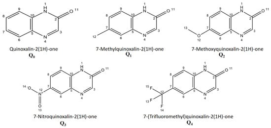
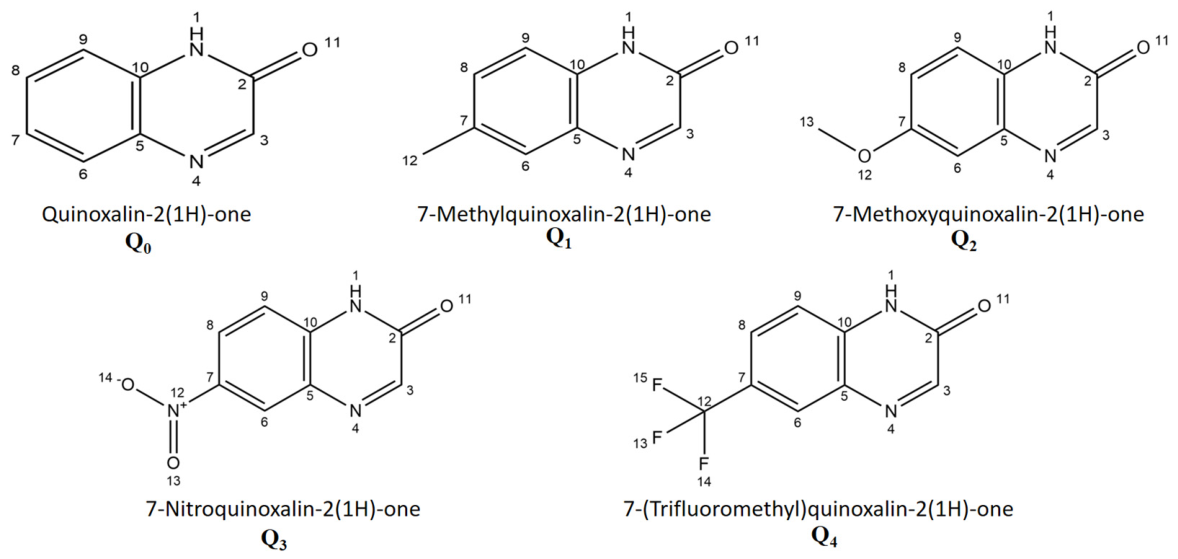
The integrated approach is employed in this study for a controlled sequence of five quinoxalin-2(1H)-one derivatives: the unsubstituted reference Q0 (H), Q1 with CH3, Q2 with OCH3, Q3 with NO2 and Q4 with CF3 (Figure 1). The substituent series was selected to introduce different levels of electron-donating and electron-withdrawing effects on the same quinoxalinone scaffold, following the conventional electronic classification of aromatic substituents [37]. The electronic and photophysical properties in twelve solvent environments, n-Hp, Sil, DPE, n-BC, THF, acetone, ACN, butanol, propanol, ethanol, methanol and water, are studied under a common CAM-B3LYP/6-311++G(d,p) framework with SMD solvation [26,30].
Figure 1.
Molecular structures and atom numbering of quinoxalin-2(1H)-one (Q0), 7-methylquinoxalin-2(1H)-one (Q1), 7-methoxyquinoxalin-2(1H)-one (Q2), 7-nitroquinoxalin-2(1H)-one (Q3), and 7-(trifluoromethyl) quinoxalin-2(1H)-one (Q4) investigated in this work.
The study combines ground-state conceptual DFT descriptions [38,39] with TD-DFT absorption involving the S0 → S1, S0 → S2 and S0 → S3 transitions, relaxation of the first excited singlet state and S1 → S0 fluorescence and vertical dipole-moment shifts.
The specific gap addressed here is therefore a controlled structure–property comparison that connects substituent-driven frontier-orbital shifts, vertical excitations, excited-state relaxation, solvatochromic response and spatial hole–electron separation on the same quinoxalinone scaffold. A fixed substitution position was chosen to isolate the electronic influence of CH3, OCH3, NO2 and CF3 rather than conflate positional and substituent effects. The contribution is an integrated and critically assessed comparison of complementary descriptors, not a claim of a new computational method or complete experimental validation. Compared with earlier work, the present study provides elements that, to our knowledge, have not yet been reported for quinoxalin-2(1H)-ones: (i) a systematic comparison of donor (CH3, OCH3) and acceptor (NO2, CF3) substituents at the same C7 position under one consistent protocol across twelve aprotic and protic solvent environments; (ii) a quantitative comparison between vertical TD-DFT dipole changes and effective Lippert–Mataga dipole changes, including an explicit treatment of the case in which the one-parameter solvatochromic model fails (Q3); and (iii) NTO/hole–electron descriptors evaluated at both the Franck–Condon and relaxed S1 geometries. Previous quinoxalinone studies were either experimental and limited to the parent compound [14], centered on synthesis and probe applications [5,6], or concerned structurally different quinoxaline and quinolinone chromophores [7,9,18].
The Onsager cavity radii obtained from the calculated molecular volumes are employed in the Lippert–Mataga regressions [40] together with the NTO-based charge redistribution characterization. The objective is to examine how substituent electronics, frontier-orbital modulation, excited-state charge transfer, solvent response, spectral shifts, and dipole reorganization are related within a single comparative framework.
Particular attention is given to whether donor and acceptor substituents reduce the electronic gap and modify excited-state polarization through different mechanisms, and to whether TD-DFT and solvatochromic descriptors provide consistent pictures of charge redistribution [4,13].
2. Materials and Methods
All calculations employed the CAM-B3LYP/6-311++G(d,p) level of theory together with the SMD implicit-solvation model [26,30]. The workflow included S0 geometry optimization and harmonic-frequency analysis, frontier-orbital and conceptual DFT calculations, LR-TD-DFT vertical absorption and equilibrium S1 optimization with state tracking and excited-state frequency verification, state-specific non-equilibrium fluorescence calculations, vector dipole-moment analysis, Onsager-cavity evaluation, Lippert–Mataga analysis, and NTO/hole-electron characterization. Wavefunction-based post-processing was performed using Multiwfn 3.8 [41,42].
The completed NTO isosurfaces were shown using GaussView 6 [43].
2.1. Molecular Systems and Solvent Set
Five quinoxalin-2(1H)-one derivatives, Q0–Q4, were selected (Figure 1, Table 1). The unsubstituted parent Q0 is compared with CH3 (Q1), OCH3 (Q2), NO2 (Q3) and CF3 (Q4) substituents at the same C7 site. Keeping the substitution position fixed allows the donor/acceptor electronic effects to be compared without conflating them with positional isomerism [37]. The relevance of substitution patterns in the quinoxalin-2-one family has been previously illustrated in a spectroscopic study of substituted quinoxalin-2-ones [44]. As a limited positional sensitivity test, a 7-methoxy versus 6-methoxy comparison in THF was additionally reported (Table S7); it does not imply that C7 is universally optimal for all substituents or solvents. The twelve solvent environments listed in Table 2 were selected for a broad orientational polarity window (Δf = −0.0012 to 0.3199) and to compare aprotic and protic environments under identical computational settings for all five compounds. This is a theoretical solvent screening, not a determination of experimental solubility; concentrations, aggregation and solution stability remain to be established experimentally.
Table 1.
Molecular systems investigated in this work (Q0–Q4).
Table 2.
Dielectric constant (ε), refractive index (n), Lippert–Mataga polarity function (Δf), and classification of the twelve solvent environments used in this study.
In this work, “silicone fluid” denotes an effective PDMS-type silicone medium (poly(dimethylsiloxane), repeat unit [–Si(CH3)2–O–]n), not a single molecule with a unique formula or a certified commercial grade. The adopted continuum parameters are ε = 2.4400 and n = 1.377 (Δf = 0.0579); these parameters should not be interpreted as measured values for a specified silicone-fluid viscosity grade. Water, methanol, ethanol, propanol and butanol are the five protic solvents in the set and can donate hydrogen bonds. Several aprotic solvents, including THF, acetone, acetonitrile and diphenyl ether, may accept hydrogen bonds from the quinoxalinone N–H group. The SMD model does not explicitly resolve such individual interactions.
2.2. Ground-State Geometry Optimization
The ground-state (S0) geometries of all Q0–Q4/solvent combinations were optimized using the CAM-B3LYP functional with the 6-311++G(d,p) basis set and the SMD solvation model [26,30].
All computations were carried out with Gaussian 09 Revision D.01 [45]. The 6-311++G(d,p) basis set was selected because it combines triple-zeta valence flexibility with both polarization and diffuse functions [46,47]. Harmonic frequency calculations were performed at the same theoretical level, and optimized S0 structures were accepted as minima only when no imaginary frequency was found. No geometrical restrictions or empirical spectral shifts have been applied. CAM-B3LYP was selected because its range-separated exchange treatment is better suited to electronic excitations involving significant spatial redistribution of electron density and charge-transfer character [25,26]. This is particularly pertinent for the substituted quinoxalinone derivatives examined here, specifically Q2 and Q3, for which the subsequent excited-state analyses demonstrate appreciable intramolecular charge-transfer character.
Additional method-sensitivity checks were reported for Q0 and Q3 in n-heptane at the 6-311++G(d,p)/SMD level using B3LYP, PBE0, CAM-B3LYP, ωB97X-D and M06-2X (Table S5). These comparisons assess vertical absorption and associated descriptors, not functional-dependent emission or relaxed-state accuracy. Selected explicit-cluster-plus-SMD checks for Q0 in water and Q2 in methanol (Table S6) and the methoxy regioisomer comparison in THF (Table S7) provide limited sensitivity tests. They do not replace experimental or high-level theoretical validation across the full molecular and solvent series.
2.3. Calculation of the Electronic Structure and Conceptual DFT Descriptors
HOMO and LUMO energies were extracted from the optimized S0 calculations. The Kohn–Sham frontier gap was evaluated as ΔEgap = ELUMO − EHOMO and treated as a ground-state comparative reactivity descriptor, distinct from the vertical optical excitation energies obtained independently from TD-DFT. A set of global conceptual DFT descriptors was subsequently derived from the frontier-orbital energies using a Koopmans-like frontier-orbital approximation to the finite-difference conceptual-DFT definitions, as reviewed by Geerlings, De Proft, and Langenaeker [48] and formalized within the density-functional framework of Parr and Yang [49]:
where χ is the global electronegativity, η the chemical hardness following the Parr–Pearson formulation [38], S the global softness, and ω the global electrophilicity index introduced by Parr, von Szentpály, and Liu [50].
These descriptors were applied identically to all Q0–Q4/solvent combinations and were treated as frontier-orbital-based comparative quantities rather than exact experimental ionization potentials or electron affinities. Their interpretation within conceptual DFT has been reviewed extensively by Chattaraj, Sarkar, and Roy [51], and related frontier-orbital/reactivity analyses have also been employed in recent computational studies from our group [39]. Definitions are summarized in Table 3.
Table 3.
Definitions of the conceptual DFT descriptors used in the analysis.
2.4. TD-DFT Absorption Calculations
Vertical singlet excitations were computed at the optimized S0 geometries by LR-TD-CAM-B3LYP/6-311++G(d,p) with SMD. Ten singlet states were requested [TD = (NStates = 10)], and the S0 → S1, S0 → S2, and S0 → S3 transitions were analyzed in detail. Vertical absorption was evaluated under the non-equilibrium solvent-response regime appropriate to a Franck–Condon excitation from an S0-equilibrated solvent environment. For each transition, the excitation energy, wavelength, oscillator strength, dominant configuration, and percentage contribution were recorded. No Tamm–Dancoff approximation was used.
2.5. Excited-State Optimization and Fluorescence
The first excited singlet state (S1) was optimized with TD-CAM-B3LYP/6-311++G(d,p)/SMD using Root = 1 under equilibrium solvation conditions. Harmonic frequency calculations were subsequently performed at the optimized S1 geometries for Q0–Q4; all verified structures showed zero imaginary frequencies. State tracking was performed during the optimization using the Root = 1 tracking procedure, with CI coefficients and NTO overlaps monitored to verify state continuity. The dominant state character was retained throughout (reported tracking/overlap criterion > 0.88), with no detected root flipping or state crossing. Vertical fluorescence S1 → S0 was then evaluated at the relaxed S1 geometry using the two-step state-specific non-equilibrium solvent-response procedure, in which the equilibrated S1 reaction field is stored and subsequently reused for the vertical de-excitation.
2.6. Dipole-Moment Analysis
Permanent dipole moments of S0 and the vertical S1–S3 states were evaluated at the same S0 geometry using the Density = Current procedure. Excited-state dipole changes were obtained from the vector difference between the Cartesian dipole components, rather than by subtracting scalar dipole magnitudes:
This vectorial definition was preferred over a simple subtraction of dipole-moment magnitudes because electronic excitation can modify both the magnitude and the spatial orientation of the molecular dipole. Particular emphasis is placed on Δμ01, because S1 is the principal emissive state considered in the fluorescence calculations.
2.7. Onsager Cavity Radius
An effective spherical Onsager radius a was determined from the molecular volume enclosed by the 0.001 a.u. electron-density isosurface, evaluated with Multiwfn 3.8 from the optimized S0 wavefunction. The corresponding effective spherical radius was obtained from a = [3 Vmol/(4π)]1/3 and one radius was retained for each derivative across its twelve solvent calculations. This procedure removes the cavity size as an adjustable regression parameter and provides a reproducible wavefunction-based definition of the volume used in the Lippert–Mataga analysis.
Because ΔμLM depends on a3, the absolute Lippert–Mataga dipole estimate is sensitive to the cavity definition. The molecular volumes and radii reported in Table 4 should therefore be interpreted specifically as 0.001 a.u. electron-density-isosurface values obtained with Multiwfn 3.8, rather than as Bondi atom-additive volumes.
Table 4.
Molecular volumes and effective Onsager cavity radii used for Q0–Q4, obtained from the 0.001 a.u. electron-density isosurface with Multiwfn 3.8 and converted to an effective spherical radius through a = [3 Vmol/(4π)]1/3.
2.8. Lippert–Mataga Analysis
For each solvent, the orientational polarity function was calculated from ε and n according to the Lippert–Mataga expression [19,20]:
Stokes shifts were calculated from the principal S0 → S1 absorption and relaxed S1 → S0 emission maxima, and linear regressions of Δ against Δf were performed using all twelve solvents for each derivative; separate aprotic and protic regressions were also inspected. The last expression above is used only when the fitted global slope m is positive, because a negative slope would make the square-root expression for ΔμLM non-real under this convention. Such a case is therefore reported as not applicable rather than replacing m by |m|.
Because a enters through a3, even positive-slope ΔμLM values remain sensitive to the cavity convention and are treated as effective solvatochromic quantities.
Alternative multiparameter solvent-polarity treatments, such as the Kamlet–Taft π*/α/β formalism [22] and the Eᴛ(30) betaine-dye scale of Reichardt [21], were not applied here but provide a natural benchmark for future refinement of the present single-parameter Lippert–Mataga treatment. Such multiparameter analyses (Catalán and Kamlet–Abboud–Taft) were recently applied to quinolin-2(1H)-one push–pull dyes, where they separated the contributions of solvent dipolarity and hydrogen-bond acidity to the emission shifts [18].
2.9. NTO and Hole–Electron Analysis
Natural Transition Orbitals were obtained using the TD-DFT transition density and examined using Multiwfn 3.8. Hole/electron analysis was carried out for Q0–Q4 at both the S0 Franck–Condon geometry and the relaxed S1 geometry. The descriptors are the hole–electron centroid separation DCT, spatial overlap S and transferred charge qCT. Larger DCT values together with reduced hole–electron overlap were interpreted as evidence of stronger charge-transfer character. The NTO hole/electron isosurfaces are plotted at a common isodensity threshold of 0.02 e/bohr3 and visualized with GaussView 6. The same visualization threshold was applied across the entire series to allow for direct qualitative comparison.
3. Results and Discussion
3.1. Solvent Polarity Function
The twelve solvent environments cover a large dielectric/optical window. The polarity function Δf of Lippert–Mataga was calculated uniformly for all derivatives using the solvent definitions and the physical constants specified in Table 2. n-Heptane provides Δf = −0.0012, silicone fluid 0.0579, diphenyl ether 0.1449, 1-chlorobutane 0.2078. Δ f contains both static-dielectric and optical-polarization terms; therefore, its ordering does not necessarily reproduce a straightforward dielectric-constant sequence. The same values of ε, n and Δf were used for Q0-Q4 so that differences in the following solvatochromic response reflect the molecular response rather than changes in solvent parametrization. The solvent set includes seven aprotic and five protic media. Such a classification is useful for the analysis of residual deviations from the global Lippert–Mataga regressions. Since the SMD calculations are continuum calculations, they do not explicitly resolve individual hydrogen bonds. Protic/aprotic differences are discussed here as solvent-environment effects and not as direct evidence for specific solute-solvent complexes. The solvent dataset and its parametrization are held fixed across the molecules; specific hydrogen-bonding and solubility effects are not directly represented.
Experimental Benchmark of Q0
For an external point of comparison, Q0 was benchmarked against the experimental 2-quinoxalinone results reported by Santra and Dogra [14]. In n-heptane, calculated absorption and emission maxima of 466 and 505 nm are red-shifted by 81 and 90 nm relative to the reported experimental maxima of 385 and 415 nm (Table 5). Equivalently, the calculated absorption and emission energies are lower by approximately 0.560 and 0.532 eV, respectively. The Stokes-shift error is smaller (1657 cm−1 calculated versus 1878 cm−1 experimental; −221 cm−1) because much of the spectral-energy offset cancels in the difference. This closer agreement does not demonstrate that the absolute excitation energies are accurate. A five-functional sensitivity comparison for Q0 in n-heptane gives absorption wavelengths between 441 and 482 nm (Table S5), with M06-2X (441 nm) closer to the experimental maximum than CAM-B3LYP (466 nm). The sources of the remaining error are not unambiguously resolved: exchange–correlation approximation, vibrational/band-shape effects, spectral-state or tautomer assignments and solvation treatment are possible contributors. Missing explicit hydrogen bonds cannot by themselves explain the n-heptane discrepancy, since n-heptane does not donate hydrogen bonds. Deviations of this size are not unusual for push–pull lactam fluorophores: for a closely related quinolin-2(1H)-one dye, TD-DFT (TPSSh/def2-TZVPP) reproduced the emission energy of one derivative within 0.5 kcal mol−1 but deviated by about 30 kcal mol−1 for its strongly accepting analog, a discrepancy attributed to the marked multiconfigurational character of its ground state [18]. The solvent-averaged calculated vertical Δμ01 of Q0 (1.83 D) is numerically similar to the experimental solvatochromic range (1.80–2.10 D), but these are not identical physical observables and their similarity is not treated as independent experimental validation. Likewise, the cavity-dependent effective ΔμLM value of 4.03 D is not equivalent to the vertical value. Accordingly, the protocol is interpreted primarily as an internally consistent means to compare molecular trends, not as a quantitatively validated predictor of absolute spectral positions.
Table 5.
Experimental comparison of Q0 in n-heptane with the literature data of Santra and Dogra [14]. The Stokes shifts were calculated from the corresponding absorption and emission wavelengths.
3.2. Electronic Structure and Conceptual DFT Descriptors
The frontier molecular orbital and conceptual DFT results (Table 6) reveal a clear dependence of the electronic structure of the quinoxalin-2(1H)-one framework on both the nature of the 7-substituent and the solvent environment. Averaging over the twelve solvents gives mean Kohn–Sham HOMO–LUMO gaps of 3.242, 3.122, 2.995, 2.830, and 3.052 eV for Q0, Q1, Q2, Q3, and Q4, respectively, giving the order Q3 < Q2 < Q4 < Q1 < Q0. Donor and acceptor substituents reach this gap reduction through different orbital mechanisms: the donor-substituted derivatives Q1 and Q2 show a progressive destabilization of the occupied frontier orbital relative to Q0, with the mean HOMO energy increasing from −6.098 eV for Q0 to −5.918 and −5.734 eV for Q1 and Q2, respectively, whereas the acceptor-substituted derivatives Q3 and Q4 exhibit pronounced LUMO stabilization, from −2.855 eV for Q0 to −3.341 eV for Q3 and −3.111 eV for Q4. The particularly low LUMO energy of Q3 is consistent with the strong electron-accepting character of the nitro substituent, in agreement with the behavior reported for NO2-containing push–pull chromophores [12].
Table 6.
Solvent-averaged frontier-orbital and conceptual DFT descriptors of Q0–Q4.
This distinction is crucial since a lower ΔEgap alone does not uniquely identify the electronic character of a chromophore. Reduced gaps are seen in both Q2 and Q3, but their electronic structures arise from opposing substituent effects, which manifest themselves later in the direction and extent of charge redistribution in the excited states (Section 3.10).
The solvent dependence of the frontier descriptors is substantial but does not follow a simple monotonic relationship with the Lippert–Mataga polarity function Δf. Across the five derivatives, the smallest frontier gaps are obtained in butanol and the largest in acetone; for example, Q3 changes from 3.147 eV in acetone to 2.578 eV in butanol. Within the present implicit-solvation framework, these variations are interpreted as arising from differential stabilization of the occupied and virtual orbitals by the SMD continuum [30], rather than as evidence for specific solvent–solute hydrogen-bond geometries.
3.3. Exceptional Electrophilic Response of the NO2-Substituted Derivative
Among the conceptual-DFT descriptors, the global electrophilicity index best differentiates Q3 [50,51]. While Q0–Q2 largely cover ω ≈ 5.47–6.76 eV and Q4 6.42–7.79 eV, Q3 covers 7.23–8.92 eV (Table 6), a range completely above that of Q0, Q1, and Q2 and only marginally overlapping with that of the significantly electron-withdrawing CF3-substituted Q4. This enhanced electrophilicity stems from the combination of high electronegativity (χ ≈ 4.76 eV) and comparatively low hardness (η ≈ 1.42 eV), rather than each characteristic independently, because ω = χ2/(2η) [50]. This behavior is in line with the low-lying LUMO of Q3 and the strong electron-withdrawing nature of NO2. This increased ground-state electrophilicity should not, however, be taken as a direct quantitative indicator of excited-state charge transfer. Q2 is illustrative of this distinction; its electrophilicity is moderate in comparison, whereas its NTO descriptors subsequently show strong donor-driven ICT (Section 3.10). Conceptual DFT and excited-state topology offer complementary rather than interchangeable representations of electronic structure and charge redistribution.
3.4. Absorption Properties and Excited-State Assignments
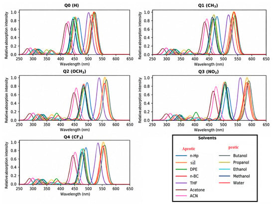
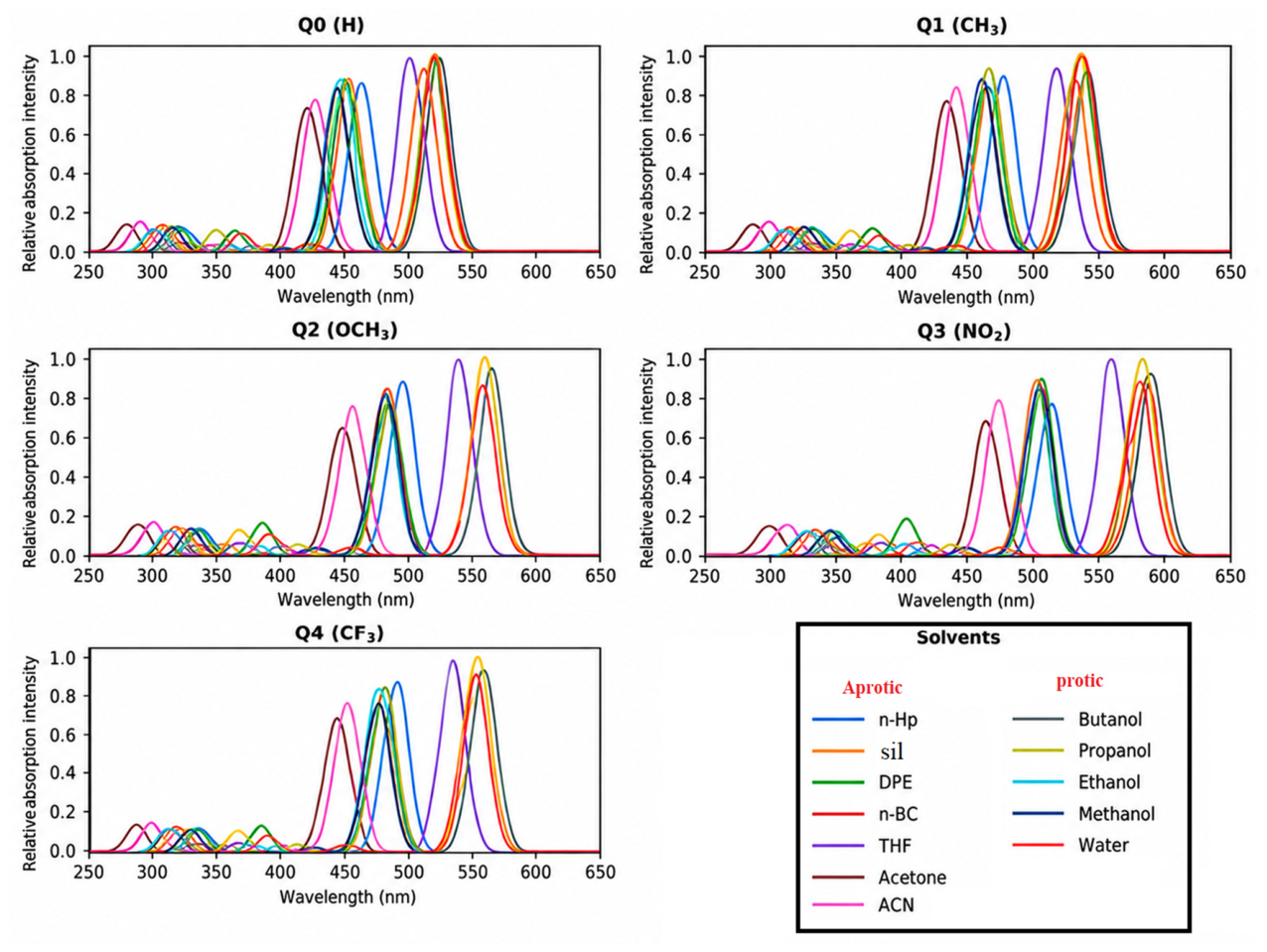
The TD-DFT computations yield the three lowest singlet electronic transitions S0 → S1, S0 → S2, and S0 → S3 for each Q0–Q4/solvent combination (Table S1, Figure 2). The oscillator-strength distribution shows that the S0 → S1 is the strongest absorption transition along the series (f S1 generally > 1) while S2 and S3 are much weaker, so that the simulated spectra show a strong long wavelength band with two weaker features at higher energy. Q0 is mainly associated with a localized π → π* excitation; Q2 receives a substantial donor-to-core charge-transfer contribution from the OCH3 substituent; and Q3 exhibits the strongest perturbation of the low-energy manifold. The S1 shows both π → π* character and pronounced charge transfer from the quinoxalinone framework to the NO2 acceptor. The computed λabs ranges for the primary S1 band are 424–525 nm (Q0), 436–543 nm (Q1), 449–563 nm (Q2), 465–591 nm (Q3) and 442–555 nm (Q4) indicating the overall bathochromic ordering Q3 > Q2 > Q4 > Q1 > Q0. However, the three transitions do not change in exactly the same way in every solvent, and the response is not strictly monotonic with Δf, indicating differential stabilization of the ground and excited states, rather than a simple one-parameter polarity dependence.
Figure 2.
Simulated TD-DFT absorption spectra of Q0–Q4 in the twelve investigated solvent environments at the CAM-B3LYP/6-311++G(d,p)/SMD level. Each spectrum was reconstructed by Gaussian broadening of the S0 → S1, S0 → S2, and S0 → S3 stick transitions using the oscillator strengths in Table S1; distinct curve colors identify the twelve solvents shown in each panel.
The complete compound-by-solvent dataset for this analysis is provided in Supplementary Table S1.
3.5. Fluorescence and Excited-State Relaxation
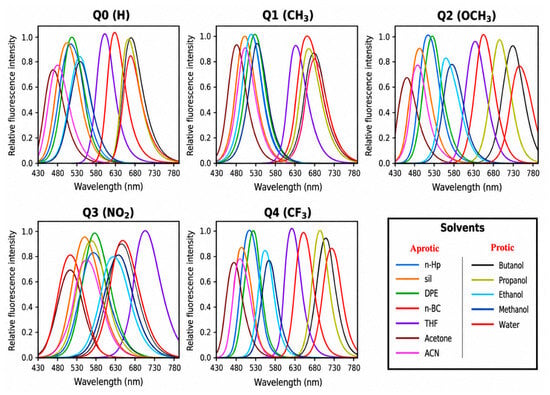
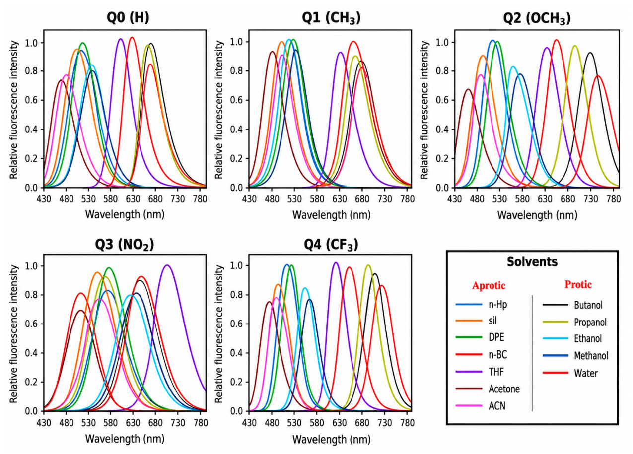
In contrast to absorption, the fluorescence analysis retains only the relaxed S1 → S0 transition (Table S2, Figure 3), evaluated after S1 geometry optimization using the state-specific and non-equilibrium solvation treatment described in Section 2.5 [33,34]. For Q0, Q1, Q2, and Q4, the emission maxima remain shifted to longer wavelengths relative to the corresponding S0 → S1 absorption maxima in all twelve solvents. The emission ranges are 474–609 nm (Q0), 491–637 nm (Q1), 522–699 nm (Q2), 545–675 nm (Q3), and 507–676 nm (Q4). The corresponding solvent-averaged emission wavelengths are 538.5, 560.5, 601.5, 592.9, and 584.3 nm, respectively, giving the mean spectral order Q2 > Q3 > Q4 > Q1 > Q0.
Figure 3.
Calculated fluorescence spectra of Q0–Q4 in the twelve investigated solvent environments from the relaxed S1 geometries at the CAM-B3LYP/6-311++G(d,p)/SMD level. Panels correspond to Q0–Q4; distinct curve colors identify the solvent-specific S1 → S0 emission profiles listed in Table S2. Intensities are shown on a relative scale for spectral comparison.
The Q3 dataset displays a more heterogeneous solvent dependence than the other derivatives. In propanol and water, λem (578 and 545 nm, respectively) is shorter than λabs (584 and 587 nm), resulting in negative apparent Stokes shifts for these two solvent environments. These values were retained without empirical adjustment and were therefore treated explicitly in the subsequent Stokes-shift and Lippert–Mataga analyses. Because such behavior is atypical for emission from a relaxed S1 state, these cases were additionally considered when assessing state tracking and the consistency of the excited-state solvation treatment.
Q0 and Q1 retain predominantly π → π* emissive character, whereas the relaxed S1 states of Q2 and Q3 exhibit more pronounced charge-transfer character, with Q4 showing intermediate behavior, consistent with the NTO/hole–electron analysis discussed in Section 3.10.
Q3 also exhibits the lowest emission oscillator-strength range of the series, with fem = 0.618–0.885, compared with 0.890–1.385 for Q0–Q2 and 0.783–1.155 for Q4. Thus, the pronounced acceptor-driven charge-transfer character inferred from the NTO/hole–electron analysis is not accompanied by an increase in transition oscillator strength. At the same time, the solvent-resolved Q3 wavelengths indicate that emission energy and charge-transfer character do not follow a simple monotonic relationship. The spatial NTO descriptors and solvent-dependent spectral response are therefore interpreted as complementary observables.
The complete compound-by-solvent dataset for this analysis is provided in Supplementary Table S2.
3.6. Stokes Shifts and Solvent-Dependent Emission
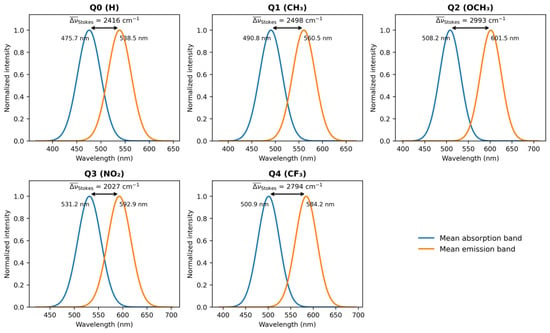
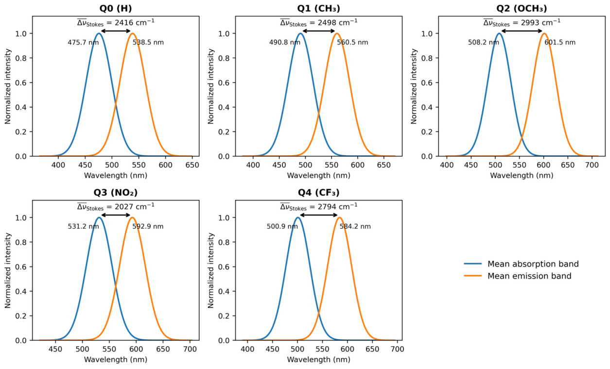
The difference between vertical S0 → S1 absorption and relaxed S1 → S0 fluorescence gives an indication of the absorption-emission separation (Table S3, Figure 4). In this data set, positive Stokes shifts are observed for 58 of the 60 Q0–Q4/solvent combinations. Q0: 1657–3019 cm−1; Q1: 1763–3063 cm−1; Q2: 1961–3679 cm−1; Q4: 1842–3455 cm−1. Q3 spans −1313 to 3515 cm−1 because the propanol and water entries give λem < λabs, corresponding to −178 and −1313 cm−1, respectively. n-BC and butanol are also substantially reduced to 1309 and 895 cm−1. The solvent-averaged Stokes shifts are found to be ~ 2416, 2498, 2993, 2027 and 2794 cm−1 for Q0-Q4, leading to the average order Q2 > Q4 > Q1 > Q0 > Q3. The highest single positive value is still that of Q2 in water (3679 cm−1). The Q3 series exhibits sign changes and strong non-monotonicity with Δf and thus it is not appropriately described as possessing the most consistently elevated Stokes response; instead the solvatochromic behavior of Q3 is considered anomalous within the single-parameter Lippert–Mataga framework.
Figure 4.
Spectral representation of the solvent-averaged absorption and emission positions for Q0–Q4. The annotated mean Stokes shifts are 2416, 2498, 2993, 2027, and 2794 cm−1 for Q0-Q4, respectively. In this solvent-averaged depiction, the average Q3 value remains positive, but the individual solvent Q3 values include negative Stokes shifts in propanol and water (Table S3).
The complete compound-by-solvent dataset for this analysis is provided in Supplementary Table S3.
3.7. Lippert–Mataga Solvatochromic Analysis
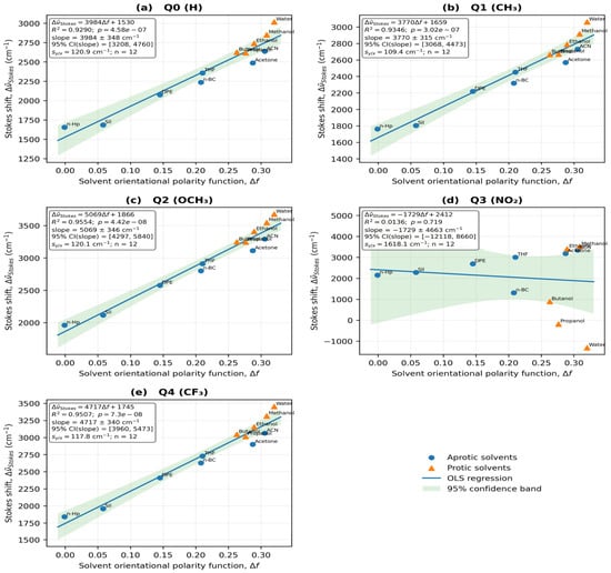
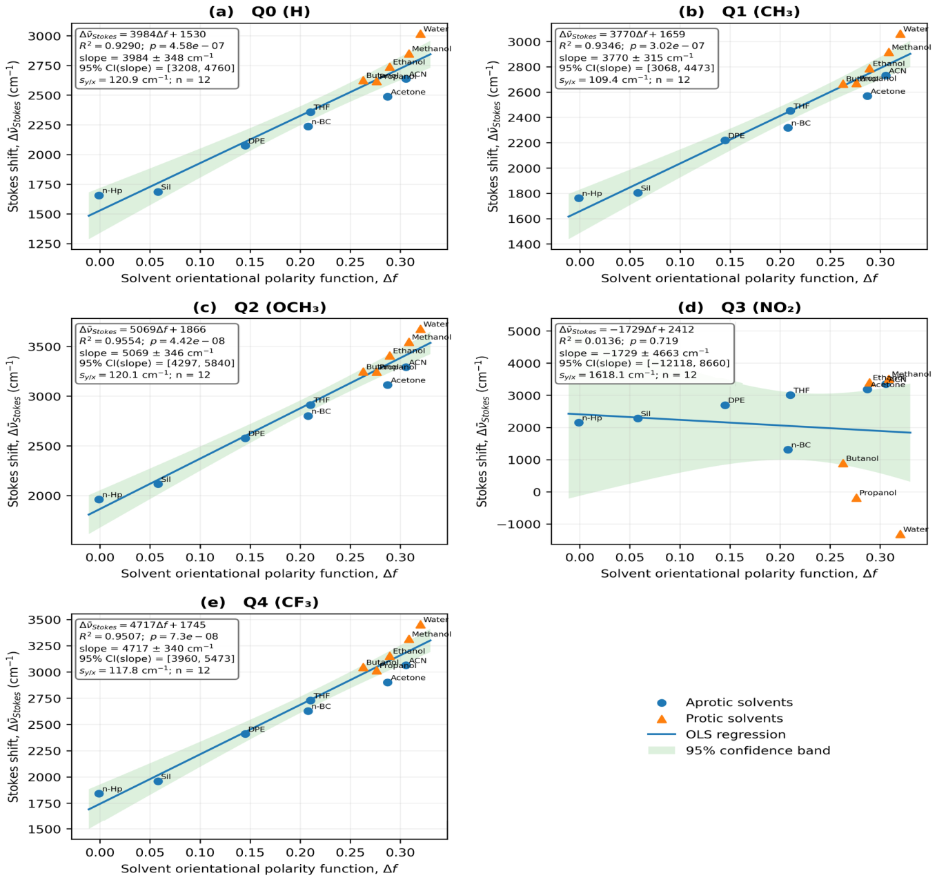
The Lippert–Mataga regressions were calculated using the Stokes-shift values of Table S3; the resulting regression parameters are collected in Table 7 and the corresponding regression plots are shown in Figure 5. Q0, Q1, Q2, and Q4 maintain strong, statistically significant global relationships: Q0, m = 3984 ± 348 cm−1 and R2 = 0.9291; Q1, 3771 ± 315 cm−1 and R2 = 0.9347; Q2, 5068 ± 346 cm−1 and R2 = 0.9555; and Q4, 4717 ± 339 cm−1 and R2 = 0.9509. The Q3 data, however, give m = −1729 ± 4663 cm−1, b = 2412 cm−1, R2 = 0.0136 and p = 0.719, with a 95% slope confidence interval that crosses both signs. The Q3 aprotic and protic subsets are also weak (R2 = 0.2617 and 0.0013, respectively). As a consequence, the emission values do not support a meaningful one-parameter linear Lippert–Mataga response for Q3, while Q2 still provides the largest positive solvatochromic slope among the valid fits.
Table 7.
Lippert–Mataga regression parameters and effective dipole-moment changes for Q0–Q4.
Figure 5.
Lippert–Mataga plots of the calculated Stokes shifts (Δ) versus the solvent orientational polarity function Δf for (a) Q0, (b) Q1, (c) Q2, (d) Q3, and (e) Q4. Each regression has twelve solvent points. Circles and triangles distinguish between aprotic and protic solvents, respectively. The global fits are significant and positive for Q0, Q1, Q2 and Q4, but a non-significant negative slope was obtained for Q3 (m = −1729 cm−1, R2 = 0.0136, p = 0.719). Q2 has the greatest valid positive slope (m = 5068 cm−1).
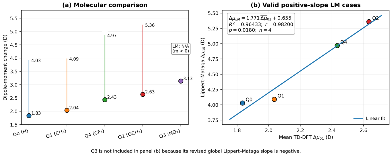
The positive global slopes for Q0, Q1, Q2, and Q4, together with the cavity radii of the 0.001 a.u. density-isosurface, yield effective ΔμLM values of 4.03, 4.09, 5.36, and 4.97 D, respectively. For Q3, the global slope is negative, so that the expression ΔμLM = (m h c a3/2)1/2 does not give a real positive dipole-change magnitude and ΔμLM is reported as not applicable rather than forcing a value through |m|. Accordingly, the present dataset does not assign any five-member Lippert–Mataga molecular ordering. This distinction does not change the direct TD-DFT or NTO results for Q3, but it removes the previous claim that the three frameworks all give the same molecular ranking.
For Q3, the global regression is statistically non-significant (m = −1729 cm−1, R2 = 0.0136, p = 0.719), and its slope uncertainty includes both signs. The two unusual pairs in propanol (584/578 nm) and water (587/545 nm) contribute strongly to the non-monotonic behavior; a negative fitted slope should therefore not be interpreted as a demonstrated inverse polarity response or as a negative physical dipole-change magnitude. Solvent-dependent relaxation or electronic-state character, specific solute–solvent interactions and errors in the excited-state solvation treatment are potential explanations, not uniquely established mechanisms. An experimental precedent exists for a structurally related scaffold: in quinolin-2(1H)-one push–pull fluorophores, hydrogen-bond donation from protic solvents inverted the emission trend of the derivative bearing the stronger acceptor, whereas the carbonyl analog retained a positive solvatochromic response [18]. Because the two anomalous Q3 entries both occur in protic media (propanol and water), such specific solute–solvent interactions, which are not described by the SMD continuum, are a plausible contributor to the deviation of Q3 from a linear Lippert–Mataga response. Independent checks of the state assignment and solvation protocol for these two fluorescence values remain important. The hole–electron centroid separation DCT and the Lippert–Mataga fit describe different observables, so the large NTO-derived charge separation of Q3 does not logically require a positive fitted global solvatochromic slope.
3.8. Excited-State Dipole-Moment Changes
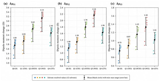
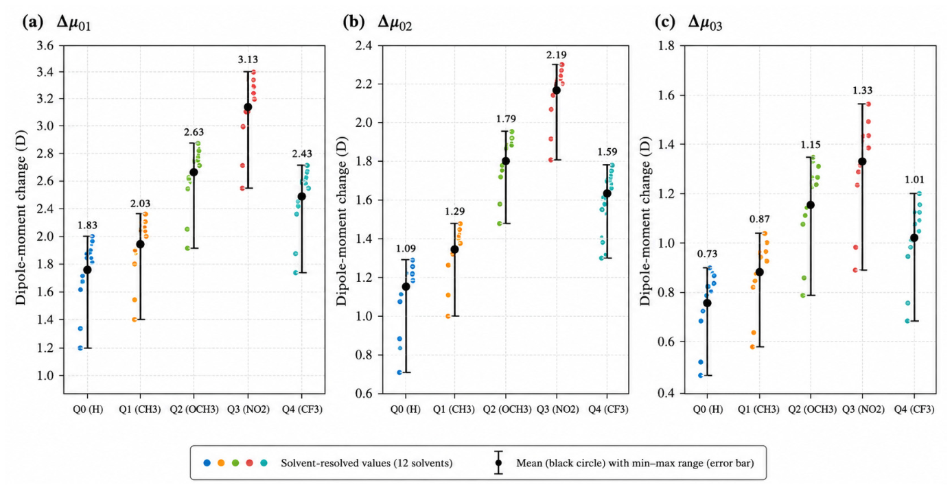
The solvent-resolved vector dipole changes given in Table S4 were calculated from the Cartesian dipole components as described in Section 2.6, and are displayed in Figure 6. The mean values of the twelve solvents are Δμ01 = 1.83, 2.03, 2.63, 3.13 and 2.43 D for Q0–Q4, respectively. The resulting molecular order is Q0 < Q1 < Q4 < Q2 < Q3. Mean Δμ 0 2 values are 1.09, 1.29, 1.79, 2.19, and 1.59 D, while mean Δμ 0 3 values are 0.73, 0.87, 1.15, 1.33, and 1.01 D. Thus, S1 consistently provides the largest dipolar reorganization, and Q3 gives the strongest response for all three low-lying singlet excitations.
Figure 6.
Solvent-resolved vertical dipole-moment changes of Q0–Q4 for (a) S0 → S1 (Δμ01), (b) S0 → S2 (Δμ02), and (c) S0 → S3 (Δμ03). Colored points represent the twelve solvent values. Black circles represent the molecular mean and the error bars represent the corresponding minimum-maximum range. The average response from S0 to S1 is Q3 > Q2 > Q4 > Q1 > Q0.
For consistency, the TD-DFT quantity used in the Lippert–Mataga comparison of Section 3.9 is the solvent-averaged vertical S0 → S1 vector quantity reported in Table 8. Only these four molecules have valid positive global Lippert–Mataga slopes, and so a numerical ΔμLM comparison is only made for Q0, Q1, Q2 and Q4. Q3 is discussed separately as its slope is negative. This definition still differs from transition-density or density-partition descriptors used in NTO/hole–electron analysis, where mixing of physically different dipole measures is avoided.
Table 8.
Solvent-averaged vertical dipole-moment changes and corresponding ranges for Q0–Q4, calculated directly from the twelve solvent-resolved values reported in Table S4.
The sample standard deviations of the twelve solvent-resolved Δμ01 values are approximately 0.29 D for each of Q0–Q4 (Table S8). These describe dispersion among the chosen solvent environments, not statistical uncertainty of the electronic-structure method or evidence that the individual-solvent responses are uniform. The NTO summaries likewise combine means with observed ranges; the fitted Lippert–Mataga ΔμLM for each compound is a regression-derived quantity rather than a solvent average.
The complete compound-by-solvent dataset for this analysis is provided in Supplementary Table S4.
3.9. TD-DFT Versus Lippert–Mataga Dipole Changes
The comparison between the direct TD-DFT dipole response and the effective Lippert–Mataga dipole change should be revisited since the updated Q3 fluorescence data gives a negative global Lippert–Mataga slope. The TD-DFT quantity is the unrounded solvent-averaged Δμ01 from Table S4 for all five molecules, but a real positive ΔμLM is available only for Q0, Q1, Q2 and Q4. Therefore, Q3 is retained in the TD-DFT/NTO mechanistic discussion but excluded from numerical TD-DFT-versus-Lippert–Mataga regression rather than assigning an artificial |m|-based value. This retains the distinction between the computed electronic polarization directly and a solvatochromic descriptor whose validity depends on the quality and sign of the solvent response fitted.
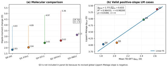
Regression of the unrounded molecular values for the four molecules with valid positive Lippert–Mataga slopes (Q0, Q1, Q2 and Q4) gives ΔμLM = 1.771 × Δ + 0.655 (R2 = 0.96433, r = 0.98200, p = 0.0180, n = 4); the molecular values are compared in Table 9 and plotted in Figure 7. This is still a strong descriptive association, but the very small molecular sample and the exclusion of Q3 do not justify presenting it as a universal cross-framework validation. Therefore, the comparison is acknowledged to indicate only a trend consistency for the four valid positive-slope cases. Clearly, Q3 shows that the NTO/TD-DFT charge-transfer character can be present even for a poor one-parameter Lippert–Mataga fit.
Table 9.
Molecular comparison of the solvent-averaged vertical TD-DFT dipole change (Δ) and the effective Lippert–Mataga dipole change (ΔμLM).
Figure 7.
Comparison between solvent-averaged TD-DFT S0 → S1 dipole changes and effective Lippert–Mataga dipole changes. The four valid positive-slope ΔμLM values and all five TD-DFT molecular means are displayed in Panel (a); Q3 is indicated as not applicable because its global Lippert–Mataga slope is negative. Panel (b) shows the descriptive correlation for four molecules for Q0, Q1, Q2 and Q4 (ΔμLM = 1.771·Δ + 0.655; R2 = 0.96433; r = 0.98200; p = 0.0180; n = 4).
3.10. NTO Analysis and Excited-State Charge Transfer
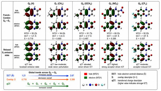
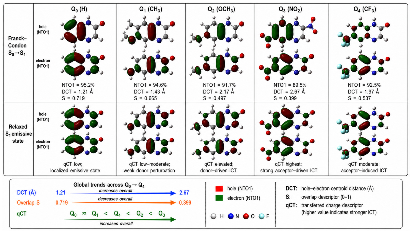
The Franck–Condon S0 → S1 transition-density descriptors and the corresponding hole/electron topology at the relaxed S1 geometry are combined in the NTO analysis (Figure 8, Table 10). At the Franck–Condon geometry, Q0 remains the most localized excitation (mean DCT = 1.21 Å, SHE = 0.719), whereas Q3 shows the largest spatial charge separation (mean DCT = 2.67 Å, SHE = 0.399). The molecular ordering derived from the mean vertical TD-DFT dipole response is consistent with the descriptor progression, which is Q0 ≈ Q1 < Q4 < Q2 < Q3 in increasing charge-transfer character. Because Q3 has no valid positive ΔμLM, the Lippert–Mataga analysis does not yield an equivalent five-molecule ordering. The relaxed-S1 analysis additionally considers S, DCT and qCT, and is reported in the Supporting Information to differentiate the vertically prepared state from the emissive relaxed-state topology. The largest mean DCT of Q3 is a transition-density descriptor and does not independently validate its solvent-dependent emission energies; its non-significant Lippert–Mataga slope should be interpreted as a limitation of the simple regression, not a contradiction resolved by assigning an unverified structural mechanism.
Figure 8.
Isosurfaces of hole and electron NTO1 at the Franck-Condon S0-S1 geometry and the relaxed S1 emissive geometry (isodensity = 0.02 e/bohr3) for Q0-Q4. For each derivative, the Franck-Condon descriptors NTO1, DCT and S are given, and the relaxed state panels show the evolution of qCT. The combination of large hole/electron overlaps in Q0 and more significant spatial separation in Q2 and especially in Q3 is consistent with the ordering Q0 ≈ Q1 < Q4 < Q2 < Q3 in terms of increasing ICT character.
Table 10.
Main S0 → S1 transition and solvent-averaged NTO and hole-electron descriptors for Q0–Q4. The twelve solvent environments studied are associated with ranges.
In Q2, the hole density is characterized by a large OCH3/adjacent π-system contribution and electron density shift to the quinoxalinone π* region, consistent with donor-to-core charge transfer. However, the clearest acceptor-directed transfer to the NO2-containing region is seen in Q3. Isosurfaces of the genuine hole/electron NTOs were generated with Multiwfn 3.8 and visualized in GaussView 6 at an isodensity threshold of 0.02 e/bohr3. The same threshold and molecular orientation were kept constant over Q0–Q4 to allow the visual comparison to represent the computed transition-density topology instead of a schematic drawing.
3.11. Integrated Structure–Property Relationship
The ground-state electronic structure, TD-DFT spectroscopy, solvatochromic analysis, dipole-moment response, experimental Q0 comparison, and NTO/hole–electron descriptors can be combined into a unified structure-property picture for Q0–Q4 (Table 11). The basic mechanistic sequence is: substituent-driven frontier-orbital perturbation-excited state charge redistribution-dipolar response-solvent stabilization-absorption/emission behavior.
Substituent → frontier-orbital perturbation → excited-state charge redistribution → dipolar response → solvent stabilization → absorption/emission behavior
Table 11.
Integrated electronic, spectroscopic, solvatochromic, and charge-transfer descriptors of Q0–Q4.
The average Kohn-Sham gaps at the ground state level decrease in the order Q3 < Q2 < Q4 < Q1 < Q0 (2.830, 2.995, 3.052, 3.122 and 3.242 eV, respectively), but the decrease is not caused by the same orbital mechanism for all substituents: the donor groups (CH3, especially OCH3) destabilize the occupied π system mainly, while the electron withdrawing substituents (NO2, CF3) stabilize the unoccupied levels preferentially (Section 3.2). Ground-state electrophilicity and excited-state charge transfer are thus complementary but not identical descriptors (Section 3.3). Q3 has extraordinarily high electrophilicity and the strongest excited-state charge separation, whereas Q2 has only modest electrophilicity but pronounced donor-driven ICT. The solvent-averaged vertical TD-DFT dipole response is Q0 < Q1 < Q4 < Q2 < Q3, whereas the NTO/hole-electron descriptors give the chemically consistent ordering Q0 ≈ Q1 < Q4 < Q2 < Q3. However, the Lippert–Mataga analysis does not reproduce this full five-molecule order. This is because Q3 has a non-significant negative global slope and therefore has no real positive ΔμLM under the adopted convention. For Q0, Q1, Q2 and Q4, the positive slope ΔμLM values are in good agreement with the TD-DFT trend. The combined picture thus distinguishes robust electronic-structure evidence for Q3 as the strongest acceptor-driven charge-transfer system from a solvent-shift regression not valid for the Q3 spectral set. Q2 is still the strongest donor-driven ICT derivative.
Thus the five derivatives cover a mechanistically differentiated landscape: Q0 and Q1 characterize the weakly perturbed reference regime, Q4 exhibits an intermediate acceptor driven response, Q2 is the strongest donor driven ICT member and Q3 the strongest acceptor driven charge-transfer response. Comparison with the Q0 experimental literature data shows a systematic bathochromic offset in absolute wavelengths but a much smaller discrepancy in the Stokes shift, supporting the use of the present calculations for comparative structure-property trends rather than precise absolute spectral prediction. These trends are pertinent to the molecular design of quinoxalinone-based sensing and donor–acceptor chromophores, but are not to be construed as direct evidence of photovoltaic or device performance in the absence of injection energetics, redox potentials, excited-state lifetimes, and device-level measurements.
4. Limitations of the Computational Model
The present model has several limitations. SMD represents solvent electrostatic and non-electrostatic effects through a continuum but does not resolve individual directional hydrogen bonds to the quinoxalinone N–H, carbonyl or substituent sites [30,32]. Five of the twelve solvents are protic hydrogen-bond donors; several aprotic solvents are potential hydrogen-bond acceptors. The limited explicit-cluster-plus-SMD checks for Q0 in water and Q2 in methanol (Table S6) show solvent-specific wavelength changes of 9–22 nm while the corresponding Stokes shifts change by less than 35 cm−1. These checks do not establish that implicit solvation is sufficient for all five derivatives or for Q3. Furthermore, experimental solubility and possible aggregation for each compound/solvent pair were not measured. Therefore the solvent series must be considered a computational screening set, not a list of experimentally verified solutions.
Second, the excited-state protocol combines non-equilibrium LR-TD-DFT absorption, equilibrium S1 optimization and state-specific non-equilibrium vertical fluorescence [33,34]. The available five-functional test for Q0 and Q3 (Table S5) demonstrates sensitivity of vertical excitation energies to the exchange–correlation functional. M06-2X provides closer agreement with the Q0 experimental absorption maximum than CAM-B3LYP within this limited comparison; however, it does not benchmark the emission energies or determine the best functional for every compound and solvent. CAM-B3LYP is retained for consistency and its range-separated treatment of charge redistribution, not because a universal superiority has been established. The sizable error of both absolute Q0 spectral maxima remains an explicit limitation.
Third, the Lippert–Mataga treatment is based on an effective Onsager cavity and a point-dipole continuum approximation [19,20]. Here the cavity radius is reproducibly obtained from the 0.001 a.u. electron density isosurface. However, the mapping of the molecular volume onto a spherical cavity is an approximation.
Fourth, the Q3 fluorescence dataset includes negative apparent Stokes shifts for propanol and water and yields a non-significant negative global Lippert–Mataga slope. This does not support assigning an effective real positive ΔμLM for Q3 under the adopted convention, nor a unique physical mechanism for the apparent anomaly. The unusual Q3 entries warrant careful independent verification of state identity and solvent-response treatment; meanwhile the NTO and solvatochromic quantities remain complementary rather than interchangeable indicators.
Finally, the study remains theoretical. Published experimental Q0 values [14] provide a limited external spectral comparison, but the differences in absolute positions prevent claims of quantitative wavelength validation. Experimental spectra and solubilities for Q1–Q4, fluorescence quantum yields and lifetimes, and solvent-specific structural data would be necessary to test the proposed molecular design implications. No quantum yield or device performance is inferred from oscillator strengths. The main contribution is a consistent, transparent comparative dataset and analysis of complementary descriptors within the stated computational framework.
5. Conclusions
This work presents an integrated computational description of the impact of 7-position substitution and the solvent environment on the ground- and excited-state behavior of the quinoxalin-2(1H)-one derivatives Q0-Q4. The method distinguishes between LR non-equilibrium vertical absorption, equilibrium S1 relaxation and state-specific non-equilibrium vertical fluorescence. The S1 minima were verified with harmonic frequency calculations and state tracking was employed to ensure that the targeted excited-state character was maintained throughout the optimization. The energetic and dipolar descriptors are complemented by NTO/hole–electron analysis at the Franck–Condon and relaxed-S1 geometries.
The results of the electronic-structure calculations show that the substituent mechanisms are clearly different. Q3 combines the smallest mean Kohn–Sham gap and highest electrophilicity with the strongest acceptor-driven charge separation, whereas Q2 exhibits the most pronounced donor-driven ICT character. The solvent-averaged vertical S0 → S1 dipole changes across the twelve solvents are 1.83, 2.03, 2.63, 3.13, and 2.43 D for Q0-Q4, respectively. The Lippert–Mataga analysis yields valid positive-slope effective values of 4.03, 4.09, 5.36, and 4.97 D for Q0, Q1, Q2, and Q4, respectively, whereas Q3 yields a non-significant negative slope (m = −1729 cm−1, R2 = 0.0136) and thus no real positive ΔμLM under the adopted convention.
The unrounded mean TD-DFT and Lippert–Mataga dipole-response values of the four molecules with valid positive Lippert–Mataga slopes show a strong descriptive association (R2 = 0.96433; r = 0.98200; p = 0.0180; n = 4), but this limited comparison is not taken as numerical equivalence or independent validation. The NTO descriptors also support the electronic mechanistic sequence, with increasing DCT, decreasing hole–electron overlap and stronger charge separation going toward Q3. Q0 and Q1 are weakly perturbed, Q4 is in the intermediate acceptor driven regime, Q2 is the major donor driven ICT derivative and Q3 is the strongest acceptor driven system despite its anomalous Lippert–Mataga response.
Overall, donor and acceptor substitution produce distinct frontier-orbital and excited-state redistribution patterns within the fixed C7 series. The calculated absolute Q0 wavelengths show substantial bathochromic deviations from experiment, and method-sensitivity checks reinforce the importance of interpreting the results comparatively. The anomalous Q3 response highlights that spatial charge-separation measures and a one-parameter solvent-polarity fit need not yield the same ordering, especially when the latter is statistically non-significant. The fully resolved solvent data and additional sensitivity checks are provided in Tables S1–S8. The novelty of the present work therefore lies not in a new electronic-structure method but in a systematic and internally consistent substituent- and solvent-resolved dataset for the quinoxalin-2(1H)-one scaffold, in which frontier-orbital, dipolar, solvatochromic and NTO descriptors are compared within one framework and their agreements and disagreements are made explicit. Experimental absorption and emission measurements for Q1–Q4 in the same solvent set, analyzed with multiparameter solvent scales as recently done for quinolin-2(1H)-one dyes [18], are the most direct next step to test the predicted trends and the anomalous behavior of Q3. These findings establish useful theoretical hypotheses and structure–property trends for future experimental examination of quinoxalinone fluorophores, without claiming validated quantum yields, experimental solubility or a new electronic-structure methodology.
Supplementary Materials
The following supporting information can be downloaded at: https://www.mdpi.com/article/10.3390/molecules31224204/s1, Table S1. Calculated TD-DFT absorption data (S0→S1, S0→S2, S0→S3) for Q0–Q4 across twelve solvent environments. Table S2. Calculated S1→S0 emission data for Q0–Q4 across twelve solvent environments. Table S3. Calculated absorption–emission separations and Stokes shifts for Q0–Q4 across twelve solvent environments. Table S4. Calculated vertical dipole-moment changes for Q0–Q4 across twelve solvent environments. Table S5. Functional sensitivity check for Q0 and Q3 in n-heptane (6-311++G(d,p)/SMD). Table S6. Explicit-micro-solvation sensitivity checks for Q0 in water and Q2 in methanol. Table S7. Comparison of position-7 versus position-6 methoxy substitution in THF. Table S8. Descriptive solvent-to-solvent variation of the three vertical dipole changes (n = 12 solvent environments per compound).
Author Contributions
Conceptualization, M.A.; methodology, M.A.; software, M.A.; validation, M.A., A.E.A. and I.R.; formal analysis, M.A.; investigation, M.A.; data curation, M.A.; writing—original draft preparation, M.A.; writing—review and editing, M.A., A.E.A., I.R., S.A.H. and K.O.K.; visualization, M.A.; supervision, A.E.A. and I.R.; project administration, I.R. All authors have read and agreed to the published version of the manuscript.
Funding
This research received no external funding. The APC was funded by Mahdi Alami.
Institutional Review Board Statement
Not applicable.
Informed Consent Statement
Not applicable.
Data Availability Statement
The calculated solvent-resolved datasets and additional comparative checks reported here are included in the article and its Supplementary Materials (Tables S1–S8). Further information and corresponding calculation records may be requested from the corresponding author.
Acknowledgments
The authors gratefully acknowledge the academic and technical support received during the preparation of this work and thank all colleagues who contributed through scientific discussions and manuscript review.
Conflicts of Interest
The authors declare no conflicts of interest.
Abbreviations
The following abbreviations are used in this manuscript:
| ACN | Acetonitrile |
| B3LYP | Becke three-parameter hybrid functional with Lee–Yang–Parr correlation |
| CAM-B3LYP | Coulomb-attenuating method applied to the B3LYP functional |
| CI | Configuration interaction |
| DCT | Hole–electron centroid separation |
| DFT | Density functional theory |
| DPE | Diphenyl ether |
| HOMO | Highest occupied molecular orbital |
| ICT | Intramolecular charge transfer |
| LE | Locally excited |
| LR | Linear response |
| LR-TD-DFT | Linear-response time-dependent density functional theory |
| LUMO | Lowest unoccupied molecular orbital |
| n-BC | 1-chlorobutane |
| n-Hp | n-heptane |
| NTO | Natural transition orbital |
| NTO1 | First (dominant) natural transition orbital pair |
| PCM | Polarizable continuum model |
| qCT | Transferred charge |
| Sil | Silicone fluid |
| SMD | Solvation model based on density |
| TD-DFT | Time-dependent density functional theory |
| THF | Tetrahydrofuran |
| N/A | Not applicable |
References
- Montana, M.; Montero, V.; Khoumeri, O.; Vanelle, P. Quinoxaline Derivatives as Antiviral Agents: A Systematic Review. Molecules 2020, 25, 2784. [Google Scholar] [CrossRef] [Scilit] [PubMed]
- Jiang, X.; Wu, K.; Bai, R.; Zhang, P.; Zhang, Y. Functionalized quinoxalinones as privileged structures with broad-ranging pharmacological activities. Eur. J. Med. Chem. 2022, 229, 114085. [Google Scholar] [CrossRef] [Scilit] [PubMed]
- Vishwakarma, V.K.; Sudhakar, A.A. Structure–property relationships of quinoxaline-based liquid crystals. Soft Matter 2021, 17, 8221–8257. [Google Scholar] [CrossRef] [Scilit] [PubMed]
- Li, X.; Hu, Y.; Sanchez-Molina, I.; Zhou, Y.; Yu, F.; Haque, S.A.; Wu, W.; Hua, J.; Tian, H.; Robertson, N. Insight into quinoxaline containing D–π–A dyes for dye-sensitized solar cells with cobalt and iodine based electrolytes: The effect of π-bridge on the HOMO energy level and photovoltaic performance. J. Mater. Chem. A 2015, 3, 21733–21743. [Google Scholar] [CrossRef] [Scilit]
- Renault, K.; Renard, P.-Y.; Sabot, C. Quinoxalin-2(1H)-ones: Chemical Synthesis, Fluorescence Properties and Applications. Eur. J. Org. Chem. 2022, 2022, e202201314. [Google Scholar] [CrossRef] [Scilit]
- Renault, K.; Renard, P.-Y.; Sabot, C. Photophysical properties of quinoxalin-2(1H)-ones: Application in the preparation of an azide-based fluorogenic probe for the detection of hydrogen sulfide. New J. Chem. 2017, 41, 10432–10437. [Google Scholar] [CrossRef] [Scilit]
- Matsumoto, S.; Takamori, M.; Akazome, M. Bathochromic Shift of Fluorescence Peak in Dipyrrolo[1,2-a:2′,1′-c]quinoxaline by Introducing Each of Electron-Donating and Electron-Withdrawing Substituent. Molecules 2023, 28, 2896. [Google Scholar] [CrossRef] [Scilit] [PubMed]
- Gerasimova, T.P.; Burganov, T.I.; Katsyuba, S.A.; Kalinin, A.A.; Islamova, L.N.; Fazleeva, G.M.; Ahmadeev, B.S.; Mustafina, A.R.; Monari, A.; Assfeld, X.; et al. Halochromic luminescent quinoxalinones as a basis for pH-sensing in organic and aqueous solutions. Dye. Pigment. 2021, 186, 108958. [Google Scholar] [CrossRef] [Scilit]
- Pawar, D.; Pandhare, R.J.; Kamble, R.M.; Dutta Choudhury, S. Polarity-Dependent Thermochromism and Solvatochromism in Aryl Substituted Quinoxalines. J. Phys. Chem. B 2025, 129, 6965–6974. [Google Scholar] [CrossRef] [Scilit] [PubMed]
- Chan, N.; Idris, A.; Abidin, Z.H.Z.; Tajuddin, H.A.; Abdullah, Z. Intramolecular charge transfer-induced solvatochromism and large Stokes shifts of furocoumarins. Mater. Chem. Phys. 2022, 276, 125406. [Google Scholar] [CrossRef] [Scilit]
- Wildervanck, M.J.; Hecht, R.; Nowak-Król, A. Synthesis and Strong Solvatochromism of Push-Pull Thienylthiazole Boron Complexes. Molecules 2022, 27, 5510. [Google Scholar] [CrossRef] [Scilit] [PubMed]
- Lee, S.; Jen, M.; Jang, T.; Lee, G.; Pang, Y. Twisted intramolecular charge transfer of nitroaromatic push–pull chromophores. Sci. Rep. 2022, 12, 6557. [Google Scholar] [CrossRef] [Scilit] [PubMed]
- de Silva, A.P.; Gunaratne, H.Q.N.; Gunnlaugsson, T.; Huxley, A.J.M.; McCoy, C.P.; Rademacher, J.T.; Rice, T.E. Signaling Recognition Events with Fluorescent Sensors and Switches. Chem. Rev. 1997, 97, 1515–1566. [Google Scholar] [CrossRef] [Scilit] [PubMed]
- Santra, S.; Dogra, S.K. Solvatochromism and prototropic reactions of 2-quinoxalinone. Chem. Phys. 1996, 207, 103–113. [Google Scholar] [CrossRef] [Scilit]
- Benali, B.; Lazar, Z.; Boucetta, A.; El Assyry, A.; Lakhrissi, B.; Massoui, M.; Jermoumi, C.; Negrier, P.; Leger, J.M.; Mondieig, D. Characterization and Spectral Study of 1,4-Dimethylquinoxaline-2,3-dione Potassium Iodide Complex. Spectrosc. Lett. 2008, 41, 64–71. [Google Scholar] [CrossRef] [Scilit]
- Tange, A.; Kishikawa, N.; Sakamoto, Y.; El-Maghrabey, M.; Wada, M.; Kuroda, N. A Turn-On Quinazolinone-Based Fluorescence Probe for Selective Detection of Carbon Monoxide. Molecules 2023, 28, 3654. [Google Scholar] [CrossRef] [Scilit] [PubMed]
- Shi, H.-X.; Bao, H.-W.; Wu, G.-Y. Solvation controlled excited-state dynamics in a donor–acceptor phenazine-imidazole derivative. RSC Adv. 2024, 14, 17071–17076. [Google Scholar] [CrossRef] [Scilit] [PubMed]
- Quintero, G.E.; Tello-Soto, A.I.; Moraga, D.; Mera-Adasme, R.; Aliaga, C.; Aliaga, M.E.; Domínguez, M. Quinolin-2(1H)-one-Based Push–Pull Fluorophores: Tuning Emission from Positive to Inverted Solvatochromism. ACS Phys. Chem. Au 2026, 6, 95–102. [Google Scholar] [CrossRef] [Scilit] [PubMed]
- Lippert, E. Dipolmoment und Elektronenstruktur von angeregten Molekülen. Z. Naturforsch. A 1955, 10, 541–545. [Google Scholar] [CrossRef] [Scilit]
- Mataga, N.; Kaifu, Y.; Koizumi, M. Solvent Effects upon Fluorescence Spectra and the Dipolemoments of Excited Molecules. Bull. Chem. Soc. Jpn. 1956, 29, 465–470. [Google Scholar] [CrossRef] [Scilit]
- Reichardt, C. Solvatochromic Dyes as Solvent Polarity Indicators. Chem. Rev. 1994, 94, 2319–2358. [Google Scholar] [CrossRef] [Scilit]
- Kamlet, M.J.; Abboud, J.L.M.; Abraham, M.H.; Taft, R.W. Linear Solvation Energy Relationships. 23. A Comprehensive Collection of the Solvatochromic Parameters, π*, α, and β, and Some Methods for Simplifying the Generalized Solvatochromic Equation. J. Org. Chem. 1983, 48, 2877–2887. [Google Scholar] [CrossRef] [Scilit]
- Becke, A.D. Density-functional thermochemistry. III. The role of exact exchange. J. Chem. Phys. 1993, 98, 5648–5652. [Google Scholar] [CrossRef] [Scilit]
- Lee, C.; Yang, W.; Parr, R.G. Development of the Colle–Salvetti correlation-energy formula into a functional of the electron density. Phys. Rev. B 1988, 37, 785–789. [Google Scholar] [CrossRef] [Scilit] [PubMed]
- Dreuw, A.; Head-Gordon, M. Failure of Time-Dependent Density Functional Theory for Long-Range Charge-Transfer Excited States: The Zincbacteriochlorin–Bacteriochlorin and Bacteriochlorophyll–Spheroidene Complexes. J. Am. Chem. Soc. 2004, 126, 4007–4016. [Google Scholar] [CrossRef] [Scilit] [PubMed]
- Yanai, T.; Tew, D.P.; Handy, N.C. A new hybrid exchange–correlation functional using the Coulomb-attenuating method (CAM-B3LYP). Chem. Phys. Lett. 2004, 393, 51–57. [Google Scholar] [CrossRef] [Scilit]
- Peach, M.J.G.; Benfield, P.; Helgaker, T.; Tozer, D.J. Excitation energies in density functional theory: An evaluation and a diagnostic test. J. Chem. Phys. 2008, 128, 044118. [Google Scholar] [CrossRef] [Scilit] [PubMed]
- Jacquemin, D.; Wathelet, V.; Perpète, E.A.; Adamo, C. Extensive TD-DFT Benchmark: Singlet-Excited States of Organic Molecules. J. Chem. Theory Comput. 2009, 5, 2420–2435. [Google Scholar] [CrossRef] [Scilit] [PubMed]
- Drzewiecka-Matuszek, A.; Rutkowska-Zbik, D. Application of TD-DFT Theory to Studying Porphyrinoid-Based Photosensitizers for Photodynamic Therapy: A Review. Molecules 2021, 26, 7176. [Google Scholar] [CrossRef] [Scilit] [PubMed]
- Marenich, A.V.; Cramer, C.J.; Truhlar, D.G. Universal Solvation Model Based on Solute Electron Density and on a Continuum Model of the Solvent Defined by the Bulk Dielectric Constant and Atomic Surface Tensions. J. Phys. Chem. B 2009, 113, 6378–6396. [Google Scholar] [CrossRef] [Scilit] [PubMed]
- Miertuš, S.; Scrocco, E.; Tomasi, J. Electrostatic interaction of a solute with a continuum. A direct utilization of ab initio molecular potentials for the prevision of solvent effects. Chem. Phys. 1981, 55, 117–129. [Google Scholar] [CrossRef] [Scilit]
- Tomasi, J.; Mennucci, B.; Cammi, R. Quantum Mechanical Continuum Solvation Models. Chem. Rev. 2005, 105, 2999–3094. [Google Scholar] [CrossRef] [Scilit] [PubMed]
- Improta, R.; Scalmani, G.; Frisch, M.J.; Barone, V. Toward effective and reliable fluorescence energies in solution by a new state specific polarizable continuum model time dependent density functional theory approach. J. Chem. Phys. 2007, 127, 074504. [Google Scholar] [CrossRef] [Scilit] [PubMed]
- Marenich, A.V.; Cramer, C.J.; Truhlar, D.G.; Guido, C.A.; Mennucci, B.; Scalmani, G.; Frisch, M.J. Practical computation of electronic excitation in solution: Vertical excitation model. Chem. Sci. 2011, 2, 2143–2161. [Google Scholar] [CrossRef] [Scilit]
- Martin, R.L. Natural transition orbitals. J. Chem. Phys. 2003, 118, 4775–4777. [Google Scholar] [CrossRef] [Scilit]
- Le Bahers, T.; Adamo, C.; Ciofini, I. A Qualitative Index of Spatial Extent in Charge-Transfer Excitations. J. Chem. Theory Comput. 2011, 7, 2498–2506. [Google Scholar] [CrossRef] [Scilit] [PubMed]
- Hammett, L.P. The Effect of Structure upon the Reactions of Organic Compounds. Benzene Derivatives. J. Am. Chem. Soc. 1937, 59, 96–103. [Google Scholar] [CrossRef] [Scilit]
- Parr, R.G.; Pearson, R.G. Absolute Hardness: Companion Parameter to Absolute Electronegativity. J. Am. Chem. Soc. 1983, 105, 7512–7516. [Google Scholar] [CrossRef] [Scilit]
- Rafiq, I.; El Assyry, A.; Hassan, S.A.; Kzar, K.O. Experimental and Theoretical Study on Hydrazine Derivatives: Structural, Electronic, and Reactivity Analysis. Mor. J. Chem. 2025, 13, 346–365. [Google Scholar] [CrossRef]
- Onsager, L. Electric Moments of Molecules in Liquids. J. Am. Chem. Soc. 1936, 58, 1486–1493. [Google Scholar] [CrossRef] [Scilit]
- Lu, T.; Chen, F. Multiwfn: A multifunctional wavefunction analyzer. J. Comput. Chem. 2012, 33, 580–592. [Google Scholar] [CrossRef] [Scilit] [PubMed]
- Lu, T. A comprehensive electron wavefunction analysis toolbox for chemists, Multiwfn. J. Chem. Phys. 2024, 161, 082503. [Google Scholar] [CrossRef] [Scilit] [PubMed]
- Dennington, R.; Keith, T.A.; Millam, J.M. GaussView, Version 6; Semichem Inc.: Shawnee Mission, KS, USA, 2016.
- Skotnicki, K.; Ostrowski, S.; Dobrowolski, J.C.; de la Fuente, J.R.; Cañete, A.; Bobrowski, K. Spectral Probe for Electron Transfer and Addition Reactions of Azide Radicals with Substituted Quinoxalin-2-Ones in Aqueous Solutions. Int. J. Mol. Sci. 2021, 22, 633. [Google Scholar] [CrossRef] [Scilit] [PubMed]
- Frisch, M.J.; Trucks, G.W.; Schlegel, H.B.; Scuseria, G.E.; Robb, M.A.; Cheeseman, J.R.; Scalmani, G.; Barone, V.; Mennucci, B.; Petersson, G.A.; et al. Gaussian 09, Revision D.01; Gaussian, Inc.: Wallingford, CT, USA, 2013.
- Krishnan, R.; Binkley, J.S.; Seeger, R.; Pople, J.A. Self-consistent molecular orbital methods. XX. A basis set for correlated wave functions. J. Chem. Phys. 1980, 72, 650–654. [Google Scholar] [CrossRef] [Scilit]
- Clark, T.; Chandrasekhar, J.; Spitznagel, G.W.; Schleyer, P.v.R. Efficient diffuse function-augmented basis sets for anion calculations. III. The 3-21+G basis set for first-row elements, Li–F. J. Comput. Chem. 1983, 4, 294–301. [Google Scholar] [CrossRef] [Scilit]
- Geerlings, P.; De Proft, F.; Langenaeker, W. Conceptual Density Functional Theory. Chem. Rev. 2003, 103, 1793–1873. [Google Scholar] [CrossRef] [Scilit] [PubMed]
- Parr, R.G.; Yang, W. Density-Functional Theory of Atoms and Molecules; Oxford University Press: New York, NY, USA, 1989. [Google Scholar]
- Parr, R.G.; von Szentpály, L.; Liu, S. Electrophilicity Index. J. Am. Chem. Soc. 1999, 121, 1922–1924. [Google Scholar] [CrossRef] [Scilit]
- Chattaraj, P.K.; Sarkar, U.; Roy, D.R. Electrophilicity Index. Chem. Rev. 2006, 106, 2065–2091. [Google Scholar] [CrossRef] [Scilit] [PubMed]

Disclaimer/Publisher’s Note: The statements, opinions and data contained in all publications are solely those of the individual author(s) and contributor(s) and not of MDPI and/or the editor(s). MDPI and/or the editor(s) disclaim responsibility for any injury to people or property resulting from any ideas, methods, instructions or products referred to in the content. |
© 2026 by the authors. Licensee MDPI, Basel, Switzerland. This article is an open access article distributed under the terms and conditions of the Creative Commons Attribution (CC BY) license.