Map–Shuffle–Reduce Arrays for Cascaded Coded Distributed Computing: Bounds and Constructions

Abstract

Cascaded coded distributed computing (CDC) reduces Shuffle communication through redundant Map computations and replicated output assignments. We propose Map–Shuffle–Reduce arrays (MSRAs), a unified framework for describing file placement, output assignment, transmitter selection, and one-shot XOR delivery. For fixed placement, assignment, and equal-length packetization, minimizing communication load is equivalent to minimizing the number of distinct array labels. We establish communication lower bounds for two settings: coded transmissions involving different file–output pairs, and the case where every output function is assigned to all nodes. We develop two cyclic MSRA constructions that attain the corresponding bounds under their respective conditions. In particular, the packetized construction achieves a communication load of $L_{\mathrm{comm}}=(K-r)/(K-1)$ when $2\le r<K$ and $K-r$ divides $K-1$, using only $N=K$ files and $Q=1$ output function. For partial output assignment, we introduce a group–helper construction that delivers complete intermediate values without splitting them into smaller packets. Under regular file storage and direct one-shot decoding using locally computed intermediate values, this construction attains a receiver-gain lower bound for its parameter family. Finally, we demonstrate how existing CDC schemes can be represented within the MSRA framework and compare their communication and implementation tradeoffs.

1. Introduction

Large-scale data processing frameworks such as MapReduce divide a computational job into Map, Shuffle, and Reduce phases, so that a large data set can be processed in parallel across multiple computing nodes [1]. In many data-intensive applications, the Shuffle phase—during which intermediate values are exchanged among nodes—can become a major communication bottleneck. Coded distributed computing (CDC) addresses this bottleneck by deliberately repeating Map computations and then exploiting coded multicast opportunities during data shuffling. The fundamental computation–communication tradeoff of CDC was characterized by Li et al. [2], and the practical relevance of coding in the Shuffle phase was further demonstrated by Coded TeraSort [3]. A broader overview of coded distributed computing and its implementation issues can be found in [4].

The cascaded CDC model extends the original setting by allowing each output function to be computed by multiple nodes. This additional redundancy can create larger multicast opportunities, but the optimal schemes in [2] require the numbers of input files and output functions to scale with combinatorial quantities such as $\left({\displaystyle \genfrac{}{}{0pt}{}{K}{r}}\right)$ and $\left({\displaystyle \genfrac{}{}{0pt}{}{K}{s}}\right)$. Such requirements may lead to large file indices, many multicast groups, and substantial code-generation and coordination overheads when the number of nodes increases. Consequently, a substantial line of work has focused on reducing implementation complexity while retaining a small communication load. Representative approaches include resolvable and other combinatorial designs [5,6,7,8,9], flexible low-complexity constructions [10], and placement-delivery-array-based schemes [11,12]. Recent grouping-based cascaded schemes further reduce the required numbers of files and output functions while maintaining one-shot binary delivery [13].

Array representations provide a useful way to expose the combinatorial structure behind coded multicast transmissions. The PDA/DPDA line of work grows out of coded caching and D2D coded caching [14,15]. Placement delivery arrays (PDAs) were introduced to jointly describe placement and delivery in coded caching [16], and related array frameworks have subsequently been used in D2D coded caching and coded distributed computing [17,18,19,20]. These works motivate a representation tailored to cascaded CDC, where an array should simultaneously describe the file-placement family, the output-function assignment family, the transmitter of each coded signal, and the one-shot decoding relation. The Map–Shuffle–Reduce array (MSRA) studied in this paper is designed for this purpose.

For fixed indexed file-placement and output-assignment patterns, an unpacketized MSRA turns one-shot Shuffle design into a label-count problem: S distinct labels represent S equal-length IV transmissions and $L_{\mathrm{comm}}=S/\left(NQ\right)$. If each IV is divided into $F_{\mathrm{IV}}$ equal-length packets, a packet-level refinement instead yields $L_{\mathrm{comm}}=S/\left(F_{\mathrm{IV}}NQ\right)$. Virtual packet rows do not increase the number N of physical files. The contribution is not merely the rewriting of established PDA constructions: we obtain new explicit designs and bounds under carefully distinguished assignment and packetization regimes.

The main contributions of this paper are summarized as follows.

• We define transmitter-labelled MSRAs for prescribed indexed placement and output-assignment families, clarify how labels multicast one IV to several receivers, and distinguish physical files from packet-level virtual rows.
• We prove a lower bound for labels appearing in at least two distinct rows and a separate unrestricted symbol-capacity bound in the all-node-assignment case. These bounds have different domains of optimality.
• We retain an unpacketized cyclic construction optimal within the multi-row-label class and give a packetized cyclic MSRA construction with $N=K$, $Q=1$ attaining the unrestricted all-node communication lower bound when $K-r\mid K-1$.
• For $1<s<K$, we construct an unpacketized group–helper MSRA with $r=ts+1$, $K=hr$ and explicit, nonuniform output assignments. All its XORs attain gain $r+s-1$ within the local-Map-side-information one-shot class. Its contribution is the combined placement, assignment, and unpacketized delivery rule, not an exclusive claim to this multicast gain. We quantify its benefit against uncoded delivery on exactly the same placement and assignments, and give qualified comparisons with existing two-round grouping.
• We discuss connections with DPDA, design-based CDC, and two-round grouping schemes, indicating which conversions preserve transmitters and which preserve only aggregate load. Section 4 compares the three constructions using matched $(K,r,s)$ where feasible, while separately reporting physical files, output functions, IV packetization, and sender balance.

• Notations: in this paper, we use the following notations unless otherwise stated. Bold capital letters, bold lowercase letters, and calligraphic fonts denote arrays, vectors, and sets, respectively. Sets are listed in increasing order; for V, let $V\left(j\right)$ denote its jth smallest element and $V\left(J\right)=\left\{V\left(j\right):j\in J\right\}$. The notation $|·|$ denotes set cardinality or vector length. For integers $a<b$, let $[a,b]=\left\{a,a+1,\dots ,b\right\}$ and $[a,b)=\left\{a,a+1,\dots ,b-1\right\}$; in particular $[1,b]=\left[b\right]$. For a finite set V, let $\left({\displaystyle \genfrac{}{}{0pt}{}{V}{t}}\right)=\left\{J\subseteq V:\left|J\right|=t\right\}$. An indexed family $\mathcal{F}={\left(F_i\right)}_{i\in \left[m\right]}$ is a sequence: different indices are retained even if corresponding sets are equal.

2. Cascaded Coded Distributed Computing System

In a cascaded coded distributed computing system, K distributed computing nodes compute Q output functions from N input files of equal size. Denote the node set, file set, and function set by $\mathcal{K}=\left[K\right]$, $\mathcal{W}=\left\{w_1,w_2,\dots ,w_N\right\}$, and $\mathcal{Q}=\left\{{\varphi }_1,{\varphi }_2,\dots ,{\varphi }_Q\right\}$, respectively. For each $q\in \left[Q\right]$, let $A_q\subseteq \mathcal{K}$ be the set of nodes assigned to compute

$$\begin{array}{cc}\hfill u_q& \triangleq {\varphi }_q(w_1,w_2,\dots ,w_N)\hfill \\ \hfill & \triangleq h_q\left(g_{q,1}\left(w_1\right),g_{q,2}\left(w_2\right),\dots ,g_{q,N}\left(w_N\right)\right),\hfill \end{array}$$

where $g_{q,n}(·)$ and $h_q(·)$ are the Map and Reduce functions, respectively. The intermediate value (IV) $v_{q,n}\triangleq g_{q,n}\left(w_n\right)$ is assumed to have T bits. For information-theoretic lower-bound statements, we use the standard independent-IV abstraction; the explicit decoding constructions do not require statistical independence of IVs. For each $n\in \left[N\right]$, let $D_n\subseteq \mathcal{K}$ denote the set of nodes storing file $w_n$. Unless otherwise stated, every file is stored by exactly r nodes and every output function is assigned to exactly s nodes, i.e., $|D_n|=r$ and $|A_q|=s$. We write the corresponding indexed families as $\mathcal{D}={\left(D_n\right)}_{n\in \left[N\right]}$ and $\mathcal{A}={\left(A_q\right)}_{q\in \left[Q\right]}$. Equal replication degrees do not by themselves imply equal file counts or equal Reduce assignments at each node; such balance is an additional condition verified separately for the explicit constructions.

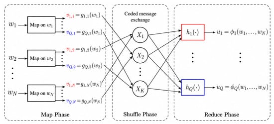
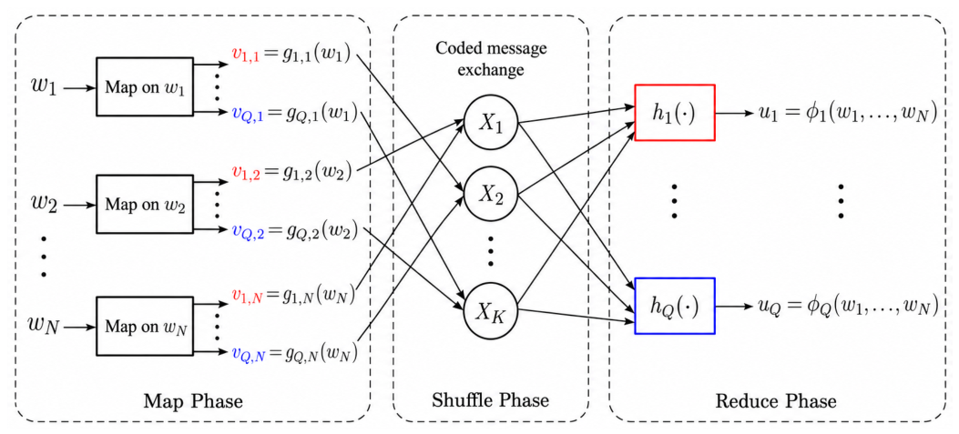
As illustrated in Figure 1, the computation consists of the following three phases.

Figure 1. Illustration of the Map, Shuffle, and Reduce phases in the cascaded coded distributed computing system.

• Map Phase. Node $k\in \mathcal{K}$ stores

  $$Z_k=\left\{w_n\mid n\in \left[N\right],k\in D_n\right\}$$

  (1)

  and computes all IVs associated with its locally stored files,

  $$I_k=\left\{v_{q,n}\mid q\in \left[Q\right],n\in \left[N\right],k\in D_n\right\}.$$

  (2)
• Shuffle Phase. If $k\in A_q$, node k needs all IVs $v_{q,n}$, $n\in \left[N\right]$, to compute $u_q$. The IVs with $k\in D_n$ are locally available, whereas those with $k\in A_q\setminus D_n$ must be obtained through communication. Let $X_k$ be the coded message transmitted by node k, generated from its locally computed IVs, and let $l_k=\left|X_k\right|$ denote its length in bits.
• Reduce Phase. After the Shuffle phase, node k recovers the missing IVs required for every assigned function and evaluates the corresponding Reduce functions to obtain all $u_q$ with $k\in A_q$.

Following [2], the computation load and communication load are defined as

$$\begin{array}{cc}\hfill r& \triangleq {\displaystyle \frac{{\sum }_{k=1}^K\left|Z_k\right|}{N}},\hfill \end{array}$$

(3)

$$\begin{array}{cc}\hfill L_{\mathrm{comm}}& \triangleq {\displaystyle \frac{{\sum }_{k=1}^K\left|X_k\right|}{QNT}}={\displaystyle \frac{{\sum }_{k=1}^K{l}_k}{QNT}}.\hfill \end{array}$$

(4)

Under $|D_n|=r$ for all $n\in \left[N\right]$, the first definition agrees with the file-replication degree.

We recall the classical symmetric cascaded CDC benchmark of Li et al. [2]. It uses each r-subset of nodes equally often for file placement and each s-subset equally often for output assignment. These uniformity requirements are stronger than $|D_n|=r$ and $|A_q|=s$ alone. The following is a benchmark for this classical symmetric model, not an asserted optimum for each arbitrary prescribed pair $(\mathcal{D},\mathcal{A})$.

Theorem 1

([2]). For $1\le r,s\le K$, suppose N and Q are positive integer multiples of $\left({\displaystyle \genfrac{}{}{0pt}{}{K}{r}}\right)$ and $\left({\displaystyle \genfrac{}{}{0pt}{}{K}{s}}\right)$, respectively, and the indexed placement and assignment families use corresponding subsets uniformly. In this symmetric setting, the classical construction achieves the benchmark communication load

$$L_{\mathrm{comm}}^{\ast }(r,s)={\displaystyle \sum _{\mathsf{\ell }=\max \left\{r+1,s\right\}}^{\min \left\{r+s,K\right\}}}{\displaystyle \frac{\left(\genfrac{}{}{0pt}{}{K-r}{\mathsf{\ell }-r}\right)\left(\genfrac{}{}{0pt}{}{r}{\mathsf{\ell }-s}\right)}{\left(\genfrac{}{}{0pt}{}{K}{s}\right)}}·{\displaystyle \frac{\mathsf{\ell }-r}{\mathsf{\ell }-1}}.$$

(5)

Here, r is the computation load and s is the number of nodes that calculate each output function.

Despite the optimality of (5) in its stated symmetric setting, the finite construction may require N and Q to scale with $\left({\displaystyle \genfrac{}{}{0pt}{}{K}{r}}\right)$ and $\left({\displaystyle \genfrac{}{}{0pt}{}{K}{s}}\right)$. For example, in the CodedTeraSort experiment [3] sorting 12 GB of data with $K=16$ workers and 100 Mbps network speed, the implementation generates file indices and initializes $\left({\displaystyle \genfrac{}{}{0pt}{}{K}{r+1}}\right)$ multicast groups for the Shuffle phase. Thus, the number of multicast groups grows combinatorially with system parameters; in the reported experiment, CodeGen overhead became dominant for sufficiently large tested computation loads. Likewise, $Q/\left({\displaystyle \genfrac{}{}{0pt}{}{K}{s}}\right)\in \mathbb{N}$ can force the output count to be a multiple of a large combinatorial quantity, which may be unsuitable for tasks with small Q. We seek structured one-shot schemes with substantially reduced file- and output-function-index scaling, while characterizing the communication cost within such low-complexity structural classes.

3. Map–Shuffle–Reduce Array

3.1. MSRA Representation and One-Shot Delivery

The indexed families $\mathcal{D}$ and $\mathcal{A}$ defined in Section 2 completely determine which nodes store each input file and which nodes are responsible for each output function. For every indexed pair $(n,q)$, a node in $D_n$ already knows $v_{q,n}$, a node in $A_q\setminus D_n$ requires $v_{q,n}$ through the Shuffle phase, and a node outside $D_n\cup A_q$ is irrelevant to that IV. We now encode these three cases, together with the transmitter and one-shot decoding relations, in a single array.

Definition 1.

For positive integers $K,N,Q,S$ and indexed families $\mathcal{A}={\left(A_q\right)}_{q\in \left[Q\right]}$ and $\mathcal{D}={\left(D_n\right)}_{n\in \left[N\right]}$ over $\left[K\right]$, consider an $NQ\times K$ array

$$\mathbf{P}={\left(p_{(D_n,A_q),k}\right)}_{n\in \left[N\right],q\in \left[Q\right],k\in \left[K\right]}.$$

Here, $(D_n,A_q)$ denotes indexed row $(n,q)$; rows with the same set values but different indices are treated as distinct rows. Each entry satisfies

$$p_{(D_n,A_q),k}=\left\{\begin{array}{cc}\ast ,\hfill & k\in D_n,\hfill \\ 0,\hfill & k\notin D_n,k\notin A_q,\hfill \\ {\sigma }^{\left(k_{\sigma }\right)},\hfill & k\notin D_n,k\in A_q,\sigma \in \left[S\right],k_{\sigma }\in \left[K\right].\hfill \end{array}\right.$$

(6)

The superscript $k_{\sigma }$ denotes the node transmitting the coded signal induced by label σ. The array is a $(K,\mathcal{D},\mathcal{A},S)$ Map–Shuffle–Reduce Array (MSRA) if for every $\sigma \in \left[S\right]$:

C0. 

${\sigma }^{\left(k_{\sigma }\right)}$ appears at least once in $\mathbf{P}$;

C1. 

${\sigma }^{\left(k_{\sigma }\right)}$ appears at most once in each column;

C2. 

if $p_{(D_n,A_q),k^{\prime }}={\sigma }^{\left(k_{\sigma }\right)}$, then $p_{(D_n,A_q),k_{\sigma }}=\ast$;

C3. 

if a label occurs at $(n_1,q_1,k_1)$ and $(n_2,q_2,k_2)$ with $(n_1,q_1)\ne (n_2,q_2)$, then the entries at $(n_1,q_1,k_2)$ and $(n_2,q_2,k_1)$ are stars.

Remark 1

(Physical meanings of entries). The symbol * means node k stores file $w_n$ and computes $v_{q,n}$; 0 means node k neither stores $w_n$ nor computes output ${\varphi }_q$; ${\sigma }^{\left(k_{\sigma }\right)}$ means node k computes ${\varphi }_q$ but lacks $w_n$ and hence requires $v_{q,n}$. For each label ${\sigma }^{\left(k_{\sigma }\right)}$, Condition C2 ensures that transmitter $k_{\sigma }$ stores the files corresponding to the indexed rows containing the label. It transmits an XOR of the distinct IVs indexed by those rows. Condition C3 ensures that every receiver can recover the requested IV using the XOR and locally available IVs; thus, delivery is one-shot.

Remark 2

(Interpretation of Conditions C0–C3). Suppose a symbol ${\sigma }^{\left(k_{\sigma }\right)}$ appears $g_{\sigma }$ times in ${\mathsf{\ell }}_{\sigma }$ distinct indexed rows, and row i contains ${\lambda }_i$ occurrences. Thus, $g_{\sigma }={\sum }_{i=1}^{{\mathsf{\ell }}_{\sigma }}{\lambda }_i$. Since C1 places the occurrences in distinct columns, grouped by row, the associated subarray has the form

$$\begin{array}{ccccccc}\hfill \hfill & \hfill {\lambda }_1\mathit{colums}\hfill & \hfill {\lambda }_2\mathit{colums}\hfill & \hfill \cdots \hfill & \hfill {\lambda }_{{\ell }_{\sigma }}\mathit{colums}\hfill & \hfill \hfill & \hfill k_{\sigma }\hfill \\ \hfill (D_{n_1},A_{q_1})\hfill & \hfill {\sigma }^{(k_{\sigma })}\hfill & \hfill \ast \hfill & \hfill \cdots \hfill & \hfill \ast \hfill & \hfill \cdots \hfill & \hfill \ast \hfill \\ \hfill (D_{n_2},A_{q_2})\hfill & \hfill \ast \hfill & \hfill {\sigma }^{(k_{\sigma })}\hfill & \hfill \cdots \hfill & \hfill \ast \hfill & \hfill \cdots \hfill & \hfill \ast \hfill \\ \hfill ⋮\hfill & \hfill ⋮\hfill & \hfill ⋮\hfill & \hfill \ddots \hfill & \hfill ⋮\hfill & \hfill ⋮\hfill & \hfill ⋮\hfill \\ \hfill (D_{n_{{\ell }_{\sigma }}},A_{q_{{\ell }_{\sigma }}})\hfill & \hfill \ast \hfill & \hfill \ast \hfill & \hfill \cdots \hfill & \hfill {\sigma }^{(k_{\sigma })}\hfill & \hfill \cdots \hfill & \hfill \ast \hfill \end{array}$$

(7)

where each displayed labelled block repeats the indicated label in all of its columns and unspecified columns are omitted. In each selected row, the transmitter and the occurrence columns belonging to all other selected rows are stars.

Theorem 2.

For any indexed file-storage family $\mathcal{D}$ whose members have cardinality r and indexed output-assignment family $\mathcal{A}$ whose members have cardinality s, a $(K,\mathcal{D},\mathcal{A},S)$ MSRA induces a cascaded CDC scheme with computation load r and communication load $L_{\mathrm{comm}}=S/\left(QN\right)$.

Proof. 

Given $\mathbf{P}$, the Map phase follows the storage and IV sets $Z_k$ and $I_k$ defined in (1)–(2). Since each $D_n$ has cardinality r, the computation load is r. For each label ${\sigma }^{\left(k_{\sigma }\right)}$, let

$$R_{\sigma }=\left\{(n,q)\in \left[N\right]\times \left[Q\right]:p_{(D_n,A_q),k^{\prime }}={\sigma }^{\left(k_{\sigma }\right)}\mathrm{for}\mathrm{some}{k}^{\prime }\in \left[K\right]\right\}.$$

The pair $(n,q)$ occurs only once in this set even when the same label appears in several columns of the row. By C2, the designated transmitter $k_{\sigma }$ stores all files associated with $R_{\sigma }$, and broadcasts

$$Y_{\sigma }=\underset{(n,q)\in R_{\sigma }}{⨁}{v}_{q,n}.$$

(8)

Consider an entry $p_{(D_{n_i},A_{q_i}),k_i}={\sigma }^{\left(k_{\sigma }\right)}$. Node $k_i\in A_{q_i}\setminus D_{n_i}$ requires $v_{q_i,n_i}$. For any other $(n,q)\in R_{\sigma }$, there is a column $k^{\prime }$ containing the same label; by C3, $p_{(D_n,A_q),k_i}=\ast$, hence $k_i\in D_n$ and node $k_i$ can compute $v_{q,n}$ locally. It therefore decodes

$$v_{q_i,n_i}=Y_{\sigma }\oplus \underset{(n,q)\in R_{\sigma }\setminus \left\{(n_i,q_i)\right\}}{⨁}{v}_{q,n}.$$

This works for all occurrences, including multiple occurrences in one row. After the Shuffle phase, each node has the IVs required for its assigned outputs. Exactly one T-bit message is transmitted for each of the S labels, so $L_{\mathrm{comm}}=ST/\left(QNT\right)=S/\left(QN\right)$. □

Definition 2

(Packet-level MSRA refinement). Let every IV $v_{q,n}$ consist of $F_{\mathrm{IV}}\ge 1$ equal-length packets $v_{q,n}^{\left(f\right)}$, $f\in \left[F_{\mathrm{IV}}\right]$, each with $T/F_{\mathrm{IV}}$ bits. Replace each indexed $(n,q)$ row by $F_{\mathrm{IV}}$ virtual $(n,f,q)$ rows with the original file-placement set $D_n$ and output assignment $A_q$. An MSRA on these $F_{\mathrm{IV}}NQ$ rows represents one-shot packet-level XOR delivery, with

$$L_{\mathrm{comm}}={\displaystyle \frac{S}{F_{\mathrm{IV}}NQ}}.$$

(9)

The physical file count remains N. A virtual row is an IV-packet index and does not assume that an arbitrary Map function applies independently to subfiles of a physical input file. We assume divisible IV symbols and equal packet lengths.

Example 1.

For $K=N=4$, $Q=1$, let $D_1=\left\{2,3\right\}$, $D_2=\left\{1,3\right\}$, $D_3=\left\{2,4\right\}$, $D_4=\left\{1,4\right\}$ and $A_1=\left[4\right]$. An MSRA is

$$\mathbf{P}=\begin{array}{ccccc}\hfill \hfill & \hfill 1\hfill & \hfill 2\hfill & \hfill 3\hfill & \hfill 4\hfill \\ \hfill (D_1,A_1)\hfill & \hfill 3^{(3)}\hfill & \hfill \ast \hfill & \hfill \ast \hfill & \hfill 2^{(2)}\hfill \\ \hfill (D_2,A_1)\hfill & \hfill \ast \hfill & \hfill 3^{(3)}\hfill & \hfill \ast \hfill & \hfill 1^{(1)}\hfill \\ \hfill (D_3,A_1)\hfill & \hfill 4^{(4)}\hfill & \hfill \ast \hfill & \hfill 2^{(2)}\hfill & \hfill \ast \hfill \\ \hfill (D_4,A_1)\hfill & \hfill \ast \hfill & \hfill 4^{(4)}\hfill & \hfill 1^{(1)}\hfill & \hfill \ast \hfill \end{array}.$$

(10)

Each label occurs in distinct columns with the required sender and cross-stars, so C0–C3 hold. Nodes store $Z_1=\left\{w_2,w_4\right\}$, $Z_2=\left\{w_1,w_3\right\}$, $Z_3=\left\{w_1,w_2\right\}$, and $Z_4=\left\{w_3,w_4\right\}$. The four coded transmissions are $X_1=v_{1,2}\oplus v_{1,4}$, $X_2=v_{1,1}\oplus v_{1,3}$, $X_3=v_{1,1}\oplus v_{1,2}$, and $X_4=v_{1,3}\oplus v_{1,4}$. Each node recovers its missing IVs; for example, node 1 computes $v_{1,1}=X_3\oplus v_{1,2}$ and $v_{1,3}=X_4\oplus v_{1,4}$. Thus, $r=2$ and $L_{\mathrm{comm}}=4/(4·1)=1$.

3.2. Transmission-Count Bounds

Theorem 3.

For any $(K,\mathcal{D},\mathcal{A},S)$ MSRA $\mathbf{P}$, where each member of $\mathcal{D}={\left(D_n\right)}_{n\in \left[N\right]}$ has cardinality $r\ge 2$ and each member of $\mathcal{A}={\left(A_q\right)}_{q\in \left[Q\right]}$ has cardinality s, put $\Gamma \triangleq {\sum }_{n=1}^N{\sum }_{q=1}^Q|A_q\setminus D_n|$. Assume $\Gamma >0$ and every labelled symbol appears in at least two distinct indexed rows. Then,

$$S\ge {\displaystyle \frac{{\Gamma }^2}{{\displaystyle (r-1)\Gamma +{\displaystyle \sum _{n=1}^N}{\displaystyle \sum _{q=1}^Q}|A_q\setminus D_n|\min \left\{|A_q\setminus D_n|,r-1\right\}}}}.$$

(11)

Proof. 

The total number of integer-labelled entries is $\Gamma$. By C0, each $\sigma \in \left[S\right]$ occurs; let $g_{\sigma }$ be its occurrence count, so ${\sum }_{\sigma }{g}_{\sigma }=\Gamma$. Suppose label $\sigma$ appears in ${\mathsf{\ell }}_{\sigma }$ distinct rows with respective multiplicities ${\lambda }_{\sigma ,1},\dots ,{\lambda }_{\sigma ,{\mathsf{\ell }}_{\sigma }}$. By Remark 2, each occurrence in row i is associated with $g_{\sigma }+1-{\lambda }_{\sigma ,i}$ distinct stars. Consequently, the integer–star association count is

$$\Omega =\sum _{\sigma \in \left[S\right]}{\displaystyle \sum _{i=1}^{{\mathsf{\ell }}_{\sigma }}}{\lambda }_{\sigma ,i}(g_{\sigma }+1-{\lambda }_{\sigma ,i})=\sum _{\sigma \in \left[S\right]}{g}_{\sigma }^2+\Gamma -\sum _{\sigma \in \left[S\right]}{\displaystyle \sum _{i=1}^{{\mathsf{\ell }}_{\sigma }}}{\lambda }_{\sigma ,i}^2.$$

(12)

Every row has exactly r stars, hence $\Omega \le r\Gamma$. Put $\Psi ={\sum }_{\sigma }{\sum }_i{\lambda }_{\sigma ,i}^2$. Then, ${\sum }_{\sigma }{g}_{\sigma }^2\le (r-1)\Gamma +\Psi$; by Cauchy–Schwarz, ${\sum }_{\sigma }{g}_{\sigma }^2\ge {\Gamma }^2/S$, yielding

$${\displaystyle \frac{{\Gamma }^2}{S}}\le (r-1)\Gamma +\Psi .$$

(13)

For each row $(n,q)$, let ${\omega }_{n,q}$ be the number of distinct labels there and let their multiplicities be $t_{n,q,1},\dots ,t_{n,q,{\omega }_{n,q}}$. Their sum is $|A_q\setminus D_n|$. Since every label spans at least two distinct rows, a label repeated t times in $(n,q)$ forces the sender column and those t occurrence columns to be stars in another row. Thus, $t\le r-1$. Therefore,

$${\displaystyle \sum _{j=1}^{{\omega }_{n,q}}}{t}_{n,q,j}^2\le |A_q\setminus D_n|\min \left\{|A_q\setminus D_n|,r-1\right\}.$$

Summing bounds $\Psi$ and substituting into (13) proves (11). □

For all-node assignment $A_q=\left[K\right]$ for each q, bound (11) becomes

$$S\ge \left\{\begin{array}{cc}{\displaystyle \frac{NQ(K-r)}{K-1}},\hfill & r>K-r,\hfill \\ {\displaystyle \frac{NQ(K-r)}{2(r-1)}},\hfill & r\le K-r.\hfill \end{array}\right.$$

(14)

Proposition 1

(Unrestricted symbol-capacity bound for all-node assignment). Suppose $A_q=\left[K\right]$ for every q, $2\le r<K$, and put $w=K-r$. Any unpacketized $(K,\mathcal{D},\mathcal{A},S)$ MSRA, without restriction on the number of rows occupied by a label, satisfies

$$S\ge {\displaystyle \frac{NQw}{\max \left\{w,r-1+\min \left\{w,r-1\right\}\right\}}}.$$

(15)

For a packet-refined MSRA, replace N by $F_{\mathrm{IV}}N$.

Proof. 

Every row has w nonstar entries, so a label confined to one row occurs at most w times. For a label present in two or more rows, choose a row with $\lambda$ occurrences and let g be its total occurrence count. The common sender column and $g-\lambda$ columns of occurrences from other rows must be distinct stars in the chosen row, by C2–C3. Hence, $g\le r-1+\lambda$. In another row, the sender and the $\lambda$ occurrence columns of the chosen row must be stars; thus, $\lambda \le r-1$, and also $\lambda \le w$. Every label covers at most $\max \left\{w,r-1+\min \left\{w,r-1\right\}\right\}$ nonstar entries; counting all $NQw$ such entries proves the claim. Packet refinement replaces N with $F_{\mathrm{IV}}N$. □

Remark 3

(Distinct optimality scopes). Theorem 3 can be sharper when all labels span at least two distinct rows. Proposition 1 also permits uncoded single-row multicast, in which one IV is requested by several nodes but transmitted once. Attaining the multi-row converse alone is not an unrestricted optimality result.

Remark 4

(Scope of optimality statements). The converse of Theorem 3 assumes each label appears in at least two distinct rows. An unrestricted MSRA may contain a label confined to one row and simultaneously requested by several nodes. Thus, optimality under (14) is asserted only for the multi-row-symbol class.

Remark 5

(Single-row benchmark for all-node assignment). When $r<K$ and $A_q=\left[K\right]$, an unrestricted MSRA admits a single-row construction with $S=NQ$ and $L_{\mathrm{comm}}=1$: for each indexed row $(n,q)$, choose $k_{n,q}\in D_n$ and put a unique label with transmitter $k_{n,q}$ in every nonstar position. Conditions C0–C2 hold and C3 is vacuous. The transmission is the full IV $v_{q,n}$. For the cyclic family below, $h=(K-1)/(r-1)$ and

$$L_{\mathrm{comm}}={\displaystyle \frac{K-r}{2(r-1)}}={\displaystyle \frac{h-1}{2}}.$$

Hence, its coded load is smaller than one when $h=2$, equal to one when $h=3$, and larger than one for $h\ge 4$. An unrestricted achievable load is $\min \left\{1,(K-r)/\left(2\right(r-1\left)\right)\right\}$. In the symmetric model of Theorem 1, $s=K$ yields $L_{\mathrm{comm}}^{\ast }(r,K)=(K-r)/(K-1)=(h-1)/h$. The cyclic-to-symmetric load ratio is therefore $h/2$, which distinguishes restricted optimality from global communication performance.

Example 2.

Let $K=3$, $N=6$, $Q=2$, $r=2$, $s=3$. Take $D_1=D_2=\left\{1,2\right\}$, $D_3=D_4=\left\{1,3\right\}$, $D_5=D_6=\left\{2,3\right\}$ and $A_1=A_2=\left[3\right]$. The following is a $(3,\mathcal{D},\mathcal{A},6)$ MSRA:

$$\mathbf{P}=\begin{array}{cccc}\hfill \hfill & \hfill 1\hfill & \hfill 2\hfill & \hfill 3\hfill \\ \hfill (D_1,A_1)\hfill & \hfill \ast \hfill & \hfill \ast \hfill & \hfill 1^{(2)}\hfill \\ \hfill (D_2,A_1)\hfill & \hfill \ast \hfill & \hfill \ast \hfill & \hfill 2^{(1)}\hfill \\ \hfill (D_2,A_1)\hfill & \hfill \ast \hfill & \hfill 2^{(1)}\hfill & \hfill \ast \hfill \\ \hfill (D_4,A_1)\hfill & \hfill \ast \hfill & \hfill 3^{(3)}\hfill & \hfill \ast \hfill \\ \hfill (D_5,A_1)\hfill & \hfill 1^{(2)}\hfill & \hfill \ast \hfill & \hfill \ast \hfill \\ \hfill (D_6,A_1)\hfill & \hfill 3^{(3)}\hfill & \hfill \ast \hfill & \hfill \ast \hfill \\ \hfill (D_1,A_2)\hfill & \hfill \ast \hfill & \hfill \ast \hfill & \hfill 4^{\left(2\right)}\hfill \\ \hfill (D_2,A_2)\hfill & \hfill \ast \hfill & \hfill \ast \hfill & \hfill 5^{\left(1\right)}\hfill \\ \hfill (D_3,A_2)\hfill & \hfill \ast \hfill & \hfill 5^{\left(1\right)}\hfill & \hfill \ast \hfill \\ \hfill (D_4,A_2)\hfill & \hfill \ast \hfill & \hfill 6^{\left(3\right)}\hfill & \hfill \ast \hfill \\ \hfill (D_5,A_2)\hfill & \hfill 4^{\left(2\right)}\hfill & \hfill \ast \hfill & \hfill \ast \hfill \\ \hfill (D_6,A_2)\hfill & \hfill 6^{\left(3\right)}\hfill & \hfill \ast \hfill & \hfill \ast \hfill \end{array}$$

(16)

Each symbol has a common sender star and cross-star pattern. Here, $|A_q\setminus D_n|=1=r-1$, so (14) gives $S\ge NQ(K-r)/(K-1)=6$, attained by this array.

3.3. Unpacketized Cyclic MSRAs

Inspired by Example 2, we present a unified class of MSRAs that attains the lower bound (14). Let $K,Q,r,N$ satisfy $2\le r<K$, $r-1\mid K-1$, and $Kh\mid N$, where $h\triangleq (K-1)/(r-1)$ and $c\triangleq N/\left(Kh\right)$. Identify the node-index set with ${\mathbb{Z}}_K=\left\{0,1,\dots ,K-1\right\}$. For every $k\in {\mathbb{Z}}_K$ and $t\in \left[h\right]$, define

$$B_{k,t}\triangleq \left\{{⟨k+t+ih⟩}_K:i\in [0,r-1)\right\},$$

(17)

where ${⟨a⟩}_K$ denotes the unique element of ${\mathbb{Z}}_K$ congruent to $a\left(\mathrm{mod}K\right)$. Since $K-1=h(r-1)$, every integer in $\left\{1,\dots ,K-1\right\}$ can be written uniquely as $t+ih$ for $t\in \left[h\right]$, $i\in [0,r-1)$. Thus, $B_{k,1},\dots ,B_{k,h}$ partition ${\mathbb{Z}}_K\setminus \left\{k\right\}$ and $|B_{k,t}|=r-1$. Define the indexed file-storage family

$$\mathcal{D}=(D_{a,k,t}:a\in \left[c\right],k\in {\mathbb{Z}}_K,t\in \left[h\right]),D_{a,k,t}\triangleq \left\{k\right\}\cup B_{k,t}.$$

(18)

Then, $\left|\mathcal{D}\right|=cKh=N$ and every placement set has cardinality r. Let

$$\mathcal{A}={\left(A_q\right)}_{q\in \left[Q\right]},A_q={\mathbb{Z}}_K.$$

(19)

For every $a\in \left[c\right]$, $q\in \left[Q\right]$, $k\in {\mathbb{Z}}_K$, and unordered pair $\left\{t,t^{\prime }\right\}\in \left({\displaystyle \genfrac{}{}{0pt}{}{\left[h\right]}{2}}\right)$, introduce a distinct label ${\sigma }_{a,q,k,\left\{t,t^{\prime }\right\}}$ with transmitter k. Define the $NQ\times K$ array by

$$p_{(D_{a,k,t},A_q),j}=\left\{\begin{array}{cc}\ast ,\hfill & j\in D_{a,k,t},\hfill \\ {\sigma }_{a,q,k,\left\{t,t^{\prime }\right\}}^{\left(k\right)},\hfill & j\in B_{k,t^{\prime }}\mathrm{for}\mathrm{some}{t}^{\prime }\in \left[h\right]\setminus \left\{t\right\}.\hfill \end{array}\right.$$

(20)

The partition property guarantees that $t^{\prime }$ in the second case is unique.

Theorem 4.

The array (20) is a $(K,\mathcal{D},\mathcal{A},S)$ MSRA with

$$S={\displaystyle \frac{NQ(K-r)}{2(r-1)}}.$$

It attains (14) and is optimal among MSRAs satisfying the multi-row-symbol hypothesis of Theorem 3. The corresponding CDC scheme has computation load r and communication load

$$L_{\mathrm{comm}}={\displaystyle \frac{K-r}{2(r-1)}}.$$

(21)

Proof. 

Every row in (20) has exactly r stars. For fixed $a,q,k$ and distinct $t,t^{\prime }$, the label ${\sigma }_{a,q,k,\left\{t,t^{\prime }\right\}}^{\left(k\right)}$ occurs in the two rows $(D_{a,k,t},A_q)$ and $(D_{a,k,t^{\prime }},A_q)$, in the columns indexed by $B_{k,t^{\prime }}$ and $B_{k,t}$, respectively. It therefore occurs (C0), and the column sets are disjoint (C1). Moreover, $k\in D_{a,k,t}\cap D_{a,k,t^{\prime }}$, giving the sender stars (C2). Columns in either $B_{k,t}$ or $B_{k,t^{\prime }}$ are stars in the other selected row, giving C3. Thus, the array is an MSRA.

The storage family is regular. Within one copy a, a node j belongs to the h sets $D_{a,j,t}$ and, for each $k\ne j$, to exactly one set $D_{a,k,t}$. Hence, it appears $c(h+K-1)$ times. The total number of distinct labels is

$$S=cKQ\left({\displaystyle \genfrac{}{}{0pt}{}{h}{2}}\right)={\displaystyle \frac{NQ(h-1)}{2}}={\displaystyle \frac{NQ(K-r)}{2(r-1)}}.$$

Since $h\ge 2$, if $h=2$ then $r>K-r$, and the first branch of (14) gives exactly this value. If $h\ge 3$, then $K-r=(h-1)(r-1)\ge 2(r-1)\ge r$, and the second branch yields the same value. The result is therefore tight within the stated multi-row-symbol class. The communication load follows from Theorem 2. □

Remark 6

(File-number scaling of the cyclic family). The smallest file number allowed by this construction is

$$N_{\min }=Kh={\displaystyle \frac{K(K-1)}{r-1}}.$$

(22)

For fixed $r\ge 3$ along admissible values of K, this grows quadratically in K, whereas $\left({\displaystyle \genfrac{}{}{0pt}{}{K}{r}}\right)=\mathsf{\Theta }\left(K^r\right)$ for the standard symmetric finite construction. For $r=2$, both counts scale quadratically, with $N_{\min }=K(K-1)=2\left({\displaystyle \genfrac{}{}{0pt}{}{K}{2}}\right)$; no asymptotic file-number reduction is claimed in that case.

Example 3.

Take $K=7$, $r=3$, $Q=1$, $N=21$, so $h=3$, $c=1$. For $k\in {\mathbb{Z}}_7$, put

$$\begin{array}{cc}\hfill B_{k,1}& =\left\{{⟨k+1⟩}_K,{⟨k+4⟩}_K\right\},\hfill \\ \hfill B_{k,2}& =\left\{{⟨k+2⟩}_K,{⟨k+5⟩}_K\right\},\hfill \\ \hfill B_{k,3}& =\left\{{⟨k+3⟩}_K,{⟨k+6⟩}_K\right\}.\hfill \end{array}$$

They partition ${\mathbb{Z}}_7\setminus \left\{k\right\}$. Set $D_{k,t}=\left\{k\right\}\cup B_{k,t}$ and $A_1={\mathbb{Z}}_7$. For each k, let $x_k^{\left(k\right)},y_k^{\left(k\right)},z_k^{\left(k\right)}$ denote labels corresponding to pairs $\left\{1,2\right\}$, $\left\{1,3\right\}$, $\left\{2,3\right\}$. With columns ordered as $k,{⟨k+1⟩}_K,\dots ,{⟨k+6⟩}_K$, the rows associated with k are

$$\left(\begin{array}{ccccccc}\ast & \ast & x_k^{\left(k\right)}& y_k^{\left(k\right)}& \ast & x_k^{\left(k\right)}& y_k^{\left(k\right)}\\ \ast & x_k^{\left(k\right)}& \ast & z_k^{\left(k\right)}& x_k^{\left(k\right)}& \ast & z_k^{\left(k\right)}\\ \ast & y_k^{\left(k\right)}& z_k^{\left(k\right)}& \ast & y_k^{\left(k\right)}& z_k^{\left(k\right)}& \ast \end{array}\right).$$

(23)

For instance, at $k=0$, the placement sets are $D_{0,1}=\left\{0,1,4\right\}$, $D_{0,2}=\left\{0,2,5\right\}$, and $D_{0,3}=\left\{0,3,6\right\}$. The common sender column and cross stars verify C0–C3. There are three labels per k, hence $S=7\left({\displaystyle \genfrac{}{}{0pt}{}{3}{2}}\right)=21$. The second branch of (14) gives $S\ge 21·4/\left[2\right(3-1\left)\right]=21$. The corresponding load is $L_{\mathrm{comm}}=21/21=1$.

Example 4.

Take $K=5$, $N=10$, $Q=1$, $r=3$, $s=5$ and the indexed family

$$\begin{array}{cccc}\hfill D_1=D_6& =\left\{1,2,3\right\},\hfill & \hfill D_2=D_7& =\left\{1,4,5\right\},\hfill \\ \hfill D_3=D_8& =\left\{2,3,4\right\},\hfill & \hfill D_4=D_9& =\left\{1,2,5\right\},\hfill \\ \hfill D_5=D_{10}& =\left\{3,4,5\right\},\hfill & & A_1=\left[5\right].\hfill \end{array}$$

The following array is a $(5,\mathcal{D},\mathcal{A},5)$ MSRA:

$$\mathbf{P}=\begin{array}{cccccc}& \hfill 1\hfill & \hfill 2\hfill & \hfill 3\hfill & \hfill 4\hfill & \hfill 5\hfill \\ \hfill (D_1,A_1)\hfill & \hfill \ast \hfill & \hfill \ast \hfill & \hfill \ast \hfill & \hfill 1^{\left(1\right)}\hfill & \hfill 1^{\left(1\right)}\hfill \\ \hfill (D_2,A_1)\hfill & \hfill \ast \hfill & \hfill 1^{\left(1\right)}\hfill & \hfill 1^{\left(1\right)}\hfill & \hfill \ast \hfill & \hfill \ast \hfill \\ \hfill (D_3,A_1)\hfill & \hfill 2^{\left(2\right)}\hfill & \hfill \ast \hfill & \hfill \ast \hfill & \hfill \ast \hfill & \hfill 2^{\left(2\right)}\hfill \\ \hfill (D_4,A_1)\hfill & \hfill \ast \hfill & \hfill \ast \hfill & \hfill 2^{\left(2\right)}\hfill & \hfill 2^{\left(2\right)}\hfill & \hfill \ast \hfill \\ \hfill (D_5,A_1)\hfill & \hfill 3^{\left(3\right)}\hfill & \hfill 3^{\left(3\right)}\hfill & \hfill \ast \hfill & \hfill \ast \hfill & \hfill \ast \hfill \\ \hfill (D_6,A_1)\hfill & \hfill \ast \hfill & \hfill \ast \hfill & \hfill \ast \hfill & \hfill 3^{\left(3\right)}\hfill & \hfill 3^{\left(3\right)}\hfill \\ \hfill (D_7,A_1)\hfill & \hfill \ast \hfill & \hfill 4^{\left(4\right)}\hfill & \hfill 4^{\left(4\right)}\hfill & \hfill \ast \hfill & \hfill \ast \hfill \\ \hfill (D_8,A_1)\hfill & \hfill 4^{\left(4\right)}\hfill & \hfill \ast \hfill & \hfill \ast \hfill & \hfill \ast \hfill & \hfill 4^{\left(4\right)}\hfill \\ \hfill (D_9,A_1)\hfill & \hfill \ast \hfill & \hfill \ast \hfill & \hfill 5^{\left(5\right)}\hfill & \hfill 5^{\left(5\right)}\hfill & \hfill \ast \hfill \\ \hfill (D_{10},A_1)\hfill & \hfill 5^{\left(5\right)}\hfill & \hfill 5^{\left(5\right)}\hfill & \hfill \ast \hfill & \hfill \ast \hfill & \hfill \ast \hfill \end{array}.$$

(24)

Each label ${\sigma }^{\left(\sigma \right)}$ occupies exactly two rows, with $D_{2\sigma -1}\cap D_{2\sigma }=\left\{\sigma \right\}$ and $D_{2\sigma -1}\cup D_{2\sigma }=\left[5\right]$. The sender and cross-star conditions follow. Since $r>K-r$, (14) gives $S\ge NQ(K-r)/(K-1)=5$, achieved by the array, and $L_{\mathrm{comm}}=5/10=1/2$.

3.4. Packetized Cyclic MSRAs

The unpacketized cyclic family in Section 3.3 is tight in the multi-row-label class, but its normalized load can exceed one. The following construction uses IV packetization to attain the all-node lower bound using only K physical files. The condition $r\ge 2$ is explicit: the one-replica boundary $r=1$ is excluded from Theorem 5 and from the corresponding use of Proposition 1.

Put $d=K-r$ and assume $2\le r<K$ and $d\mid K-1$. Let $f=(K-1)/d$, and index both nodes and files by ${\mathbb{Z}}_K$. For file $w_n$, set

$$B_n=\left\{{⟨n+1⟩}_K,\dots ,{⟨n+d⟩}_K\right\},D_n={\mathbb{Z}}_K\setminus B_n.$$

(25)

Take $N=K$, $Q=1$, $A_1={\mathbb{Z}}_K$, and divide each IV $v_n=v_{1,n}$ into $F_{\mathrm{IV}}=f$ packets $v_n^{\left(j\right)}$, $j\in [0,f)$. Node y broadcasts one packet-length XOR

$$X_y={\displaystyle \underset{j=0}{\overset{f-1}{⨁}}}{v}_{{⟨y+jd⟩}_K}^{\left(j\right)},y\in {\mathbb{Z}}_K.$$

(26)

Theorem 5

(Packetized all-node cyclic construction). For $K\ge 3$, $2\le r<K$, and $d=K-r\mid K-1$, delivery (26) has a valid packet-level MSRA representation with $S=K$ labels and

$$N=K,Q=1,s=K,F_{\mathrm{IV}}={\displaystyle \frac{K-1}{K-r}},L_{\mathrm{comm}}={\displaystyle \frac{K-r}{K-1}}.$$

(27)

It attains Proposition 1 and the all-node communication lower bound. Among regular placements for the given $K,r$, $N=K$ is the smallest positive physical file count. Conditional on $N=K$, $Q=1$, and equal-length packet transmissions, $F_{\mathrm{IV}}=(K-1)/d$ is the smallest packetization compatible with this load.

Proof. 

Fix a sender y. The sets $B_{{⟨y+jd⟩}_K}$, $j\in [0,f)$, partition ${\mathbb{Z}}_K\setminus \left\{y\right\}$: they consist of the $df=K-1$ consecutive modular positions other than y. Node y stores every file occurring in $X_y$. Each other node misses exactly one of these files, knows all other packets in the XOR, and decodes the requested packet in one shot. For each file n and packet index j, exactly one sender $y={⟨n-jd⟩}_K$ includes $v_n^{\left(j\right)}$, so every missing packet is delivered once to its requesting nodes.

Equivalently, introduce a label $z_y^{\left(y\right)}$ in the columns $B_{{⟨y+jd⟩}_K}$ of virtual row $({⟨y+jd⟩}_K,j,1)$ for each j. The missing sets are disjoint (C1), the sender stores all files (C2), and cross entries are stars (C3); every label occurs (C0). Since $S=K$, (9) gives $L_{\mathrm{comm}}=K/\left(fK\right)=d/(K-1)$.

Each physical file is stored at r nodes and each node stores r of the K files. Since $K=df+1$ and $r=K-d$, we have $\gcd (K,r)=\gcd (K,d)=1$. Any regular placement with $N^{\prime }$ physical files and M files per node must satisfy $N^{\prime }r=KM$, implying $K\mid N^{\prime }$ and $N^{\prime }\ge K$. If $N=K$, $Q=1$, and an equal-length packet scheme with factor $F^{\prime }$ attains load $1/f$, then its transmission count $S=K{F}^{\prime }/f$ must be an integer. As $\gcd (K,f)=1$, $f\mid F^{\prime }$, establishing minimality of $F^{\prime }$.

Proposition 1 on the $fK$ virtual packet rows gives $S\ge fKd/(K-1)=K$, which is achieved. Independently, let $M_k$ denote the number of files held by node k. In the independent-IV converse, node k needs $Q(N-M_k)$ IVs from other nodes, so ${\sum }_{j\ne k}\left|X_j\right|\ge Q(N-M_k)T$. Summing over k gives $(K-1){\sum }_j\left|X_j\right|\ge QN(K-r)T$, i.e., $L_{\mathrm{comm}}\ge (K-r)/(K-1)$. □

Example 5

(Thirteen nodes and four IV packets). Take $K=13$, $r=10$, $d=3$, and $f=4$. Then, $N=13$, $Q=1$, $S=13$, and $L_{\mathrm{comm}}=1/4$. For $y=0$, the files $0,3,6,9$ have missing-node sets $\left\{1,2,3\right\}$, $\left\{4,5,6\right\}$, $\left\{7,8,9\right\}$, and $\left\{10,11,12\right\}$, respectively. Node 0 transmits $X_0=v_0^{\left(0\right)}\oplus v_3^{\left(1\right)}\oplus v_6^{\left(2\right)}\oplus v_9^{\left(3\right)}$. Each other node decodes precisely one missing packet using its locally available packets. The analogous broadcasts of all other senders complete the delivery.

Remark 7

(Overlap of the two cyclic families). The unpacketized family requires $K-1=h(r-1)$ with integer $h\ge 2$, while the packetized family requires $K-r\mid K-1$. Under the first condition, $K-r=(h-1)(r-1)$; simultaneous admissibility requires $h-1\mid h$, so $h=2$, or $K=2r-1$. At these common parameters, both loads are $1/2$. The unpacketized family uses $N_{\min }=2K$ physical files without packetization, while Theorem 5 uses $N=K$ and $F_{\mathrm{IV}}=2$. The packetized family is not available at $h\ge 3$. The unpacketized load $(h-1)/2$ equals uncoded single-row multicast at $h=3$ and exceeds it at $h\ge 4$; its significance in those regimes is restricted multi-row attainability, not an unrestricted communication improvement.

3.5. Group–Helper MSRAs for Partial Output Assignment

We now consider $1<s<K$. Let $s\ge 2$, $t\ge 1$, $h\ge 2$, and put

$$r=ts+1,K=hr,g=ht.$$

(28)

Partition $gs$ nodes into g disjoint sets $G_1,\dots ,G_g$ of size s, leaving h helpers $y_1,\dots ,y_h$. For each helper $a\in \left[h\right]$ and t-subset $T\subseteq \left[g\right]$, introduce a physical file stored at

$$D_{a,T}=\left\{y_a\right\}\cup \bigcup _{j\in T}{G}_j.$$

(29)

For each $j\in \left[g\right]$, introduce one output assigned to $A_j=G_j$. For each helper a and $(t+1)$-subset $U\subseteq \left[g\right]$, introduce a label $z_{a,U}^{\left(y_a\right)}$; it occupies all s columns of $G_j$ in row $(D_{a,U\setminus \left\{j\right\}},A_j)$, for each $j\in U$. All other entries are stars or zeros as in Definition 1.

Lemma 1

(Local-Map-side-information one-shot receiver-gain bound). Consider a single XOR of distinct, independent, equal-length IV packets. The sender forms the XOR exclusively from IV packets computed from its locally stored physical files. Each intended receiver must recover its required packet directly from this XOR and IV packets computed from its own locally stored files, without using packets decoded from other transmissions. For each XOR component i, let $R_i$ be the nonempty set of nodes recovering that component. If each physical file is stored at exactly r nodes and each output is assigned to exactly s nodes, then the number of receiver–packet demands served by this XOR obeys

$$\sum _i\left|R_i\right|\le \min \left\{r+s-1,K-1\right\}.$$

(30)

Proof. 

Because the demanded packets are independent and recovery is direct from a single XOR using only local Map-side information, a receiver cannot recover two packets that are both unknown to it. Hence, the sets $R_i$ are pairwise disjoint. For any component i, the sender stores its underlying physical file, and each receiver in $R_j$, $j\ne i$, must also store that file to cancel component i. The sender is distinct from all intended receivers, so $1+{\sum }_{j\ne i}\left|R_j\right|\le r$. Moreover, $R_i$ consists of nodes assigned to the output function of component i, giving $|R_i|\le s$. Choosing any nonempty $R_i$ yields ${\sum }_j|R_j|\le r-1+|R_i|\le r+s-1$. Finally, a sender can serve at most the other $K-1$ nodes in one broadcast. This proves the bound. It is not a converse for schemes using previously decoded side information, joint multi-transmission decoding, or general nonlinear/network codes. □

Theorem 6

(Unpacketized group–helper MSRA). The placement and label rule in (28)–(29) define a binary one-shot MSRA with

$$\begin{array}{cc}\hfill N& =h\left({\displaystyle \genfrac{}{}{0pt}{}{ht}{t}}\right),Q=ht,F_{\mathrm{IV}}=1,\hfill \\ \hfill S& =h\left({\displaystyle \genfrac{}{}{0pt}{}{ht}{t+1}}\right),L_{\mathrm{comm}}={\displaystyle \frac{h-1}{h(t+1)}}.\hfill \end{array}$$

(31)

Every transmitted XOR serves $(t+1)s=r+s-1$ node–IV demands. Among schemes with the same $(K,r,s)$, regular file storage, and independent equal-length IV packets delivered by locally generated XORs with direct one-shot decoding from local Map-side information as specified in Lemma 1, the scheme meets the receiver-gain counting lower bound. This is not an optimum over arbitrary coded or multi-round delivery strategies, and the assignment family is not uniform over all s-node subsets.

Proof. 

Each file is stored at $ts+1=r$ nodes. A helper $y_a$ belongs to $\left({\displaystyle \genfrac{}{}{0pt}{}{g}{t}}\right)$ files, and a group node belongs to $h\left({\displaystyle \genfrac{}{}{0pt}{}{g-1}{t-1}}\right)=\left({\displaystyle \genfrac{}{}{0pt}{}{g}{t}}\right)$ files because $g=ht$; thus, storage is regular. For a label $z_{a,U}^{\left(y_a\right)}$, its receiver groups $G_j$, $j\in U$, are disjoint (C1), its helper stores all corresponding files (C2), and row $U\setminus \left\{j\right\}$ contains stars in every other group $G_k$, $k\in U\setminus \left\{j\right\}$ (C3). Each label appears (C0), so every receiver decodes one desired IV, and every message serves $(t+1)s$ receivers.

There are $S=h\left({\displaystyle \genfrac{}{}{0pt}{}{g}{t+1}}\right)$ labels and $N=h\left({\displaystyle \genfrac{}{}{0pt}{}{g}{t}}\right)$ files, hence

$$L_{\mathrm{comm}}={\displaystyle \frac{h\left(\genfrac{}{}{0pt}{}{g}{t+1}\right)}{h\left(\genfrac{}{}{0pt}{}{g}{t}\right)g}}={\displaystyle \frac{g-t}{g(t+1)}}={\displaystyle \frac{h-1}{h(t+1)}}.$$

Under regular storage, each node stores $M=Nr/K$ files. There are $Qs(N-M)=NQs(K-r)/K$ receiver–IV demands. Dividing by the maximum one-shot gain $r+s-1$ from Lemma 1 gives

$$L_{\mathrm{comm}}\ge {\displaystyle \frac{s(K-r)}{K(r+s-1)}}={\displaystyle \frac{h-1}{h(t+1)}},$$

with equality under (28). Here, $(t+1)s\le K-1$, so the construction also meets the $K-1$ receiver cap in Lemma 1. The counting converse assumes local Map-side-information one-shot XOR decoding and equal-length independent IV packets; it does not cover joint decoding across transmissions or arbitrary multi-round or nonlinear coding. □

Example 6

(Partial-assignment construction). Take $(s,t,h)=(2,2,2)$, so $(K,r,s)=(10,5,2)$ and $g=4$. The group–helper scheme uses $N=12$ files, $Q=4$ functions, $S=8$ full-IV XORs and $L_{\mathrm{comm}}=1/6$. The two-round grouping construction of [13] at the same $(K,r,s)$ uses $(N,Q,F_{\mathrm{IV}},S,L_{\mathrm{comm}})=(60,5,3,180,1/5)$; see Appendix B. The same-placement uncoded baseline is given next.

Remark 8

(Same-instance uncoded multicast). For the group–helper placement (29), file $(a,T)$ is stored at helper $y_a$ and groups indexed by T. For each output group $G_j$ with $j\notin T$, the entire group requests the same IV, which $y_a$ may transmit uncoded once. Exactly $N(g-t)$ full-IV transmissions suffice for the same physical files and output-assignment family, giving

$$L_{\mathrm{uncoded},\mathrm{same}}={\displaystyle \frac{N(g-t)}{NQ}}={\displaystyle \frac{h-1}{h}},{\displaystyle \frac{L_{\mathrm{uncoded},\mathrm{same}}}{L_{\mathrm{group}-\mathrm{helper}}}}=t+1.$$

(32)

At $(10,5,2)$ this is 24 uncoded messages (load $1/2$) rather than eight XORs (load $1/6$), a two-thirds reduction in transmitted bits for identical demands, not a claim about wall-clock time.

Remark 9

(Constructive contribution versus earlier two-round grouping). The two-round grouping construction of [13] already achieves receiver gain $r+s-1$ in one of its rounds; achieving that gain in isolation is therefore not claimed as a new multicast principle. The distinct contribution of Theorem 6 is a specified joint family of regular file placements, group-only (rather than symmetric) output assignments, and helper-generated, unpacketized XORs, all attaining this gain. On the identical $(\mathcal{D},\mathcal{A})$, Remark 8 proves an exact factor-$t+1$ reduction relative to uncoded multicast. For the common subfamily $h=s=2$, the comparison with [13] is analytic: both use $(K,r,s)=(4t+2,2t+1,2)$, while

$${\displaystyle \frac{N_{\mathrm{TG}}}{N_{\mathrm{GH}}}}=2t+1,{\displaystyle \frac{L_{\mathrm{GH}}}{L_{\mathrm{TG}}}}={\displaystyle \frac{2t+1}{2t+2}},(Q_{\mathrm{GH}},Q_{\mathrm{TG}})=(2t,2t+1),$$

and $(F_{\mathrm{IV},\mathrm{GH}},F_{\mathrm{IV},\mathrm{TG}})=(1,t+1)$. The latter comparison holds at matching $(K,r,s)$ but not at identical output counts or indexed assignments, so it is a parameter tradeoff rather than a same-task dominance theorem. The group–helper arrangement also incurs the sender and Reduce imbalance described next.

Remark 10

(Peak transmitter load and assignment imbalance). Each of the h helpers transmits $\left({\displaystyle \genfrac{}{}{0pt}{}{g}{t+1}}\right)$ full-IV XORs, while every non-helper transmits none. Thus, maximum-to-average sender load is

$${\displaystyle \frac{{\max }_{k\in \left[K\right]}\left|X_k\right|}{K^{-1}{\sum }_{k\in \left[K\right]}\left|X_k\right|}}={\displaystyle \frac{K}{h}}=r.$$

(33)

At $(10,5,2)$, each helper sends four messages and the other eight nodes send none, giving ratio five. Storage is balanced, but Reduce assignments are not: each group node handles one output and helpers handle none. Lower aggregate traffic does not establish lower latency or balanced computation.

4. Performance and Complexity Comparison with Existing CDC Schemes

We compare Theorems 4–6 with representative PDA- and design-based CDC schemes [5,6,7,8,9,10,11,12,13] in terms of the physical file count N, output-function count Q, output replication factor s, and normalized communication load $L_{\mathrm{comm}}$. When packetization is used, we also list $F_{\mathrm{IV}}$. Following the comparison approach of [9], numerical examples are evaluated at identical $(K,r,s)$ wherever the published parameter conditions allow. Such examples need not represent the same file placement or output-function assignment. Several schemes in [5,6,7,8,10,12] are specialized to nonmatching assignment or combinatorial-design regimes and do not provide verified instances at the matched parameter points selected below. Rather than force an artificial numerical comparison, we focus on the applicable PDA construction [11], the design-based construction [9], and the grouping construction [13], with the classical symmetric-subset benchmark [2] as a reference. The scalar load $L_{\mathrm{comm}}$ normalizes total transmitted bits by each scheme’s own $NQT$; a smaller value at matched $(K,r,s)$ alone does not establish better performance on an identical set of files, Reduce tasks, or transmitter capacities. For packetized schemes, S denotes equal-length packet transmissions in the MSRA representation, which need not equal the number of physical broadcasts in the original implementation.

4.1. All-Node Output Assignment ($s=K$)

For Theorem 4, let $h=(K-1)/(r-1)\ge 2$ be an integer. With its minimum file count, the unpacketized construction gives

$$N_4=Kh,Q_4=1,F_{\mathrm{IV},4}=1,L_4={\displaystyle \frac{h-1}{2}}.$$

(34)

Theorem 5 instead requires $K-r\mid K-1$ and achieves

$$N_5=K,Q_5=1,F_{\mathrm{IV},5}={\displaystyle \frac{K-1}{K-r}},L_5={\displaystyle \frac{K-r}{K-1}}.$$

(35)

Table 1 summarizes these constructions and comparable PDA schemes. The classical benchmark is included as a communication reference, although its symmetric-subset placement generally uses more files.

Table 1. Parametric comparison for the all-node-output case $s=K$ and $Q=1$. For PDA Scheme 2, $r\mid K$; Theorem 4 requires $r-1\mid K-1$ and Theorem 5 requires $K-r\mid K-1$. The displayed PDA loads refer to their coded branches.

Scheme	N	Q	s	${\mathit{F}}_{\mathbf{IV}}$	${\mathit{L}}_{\mathbf{comm}}$
Theorem 4	$Kh$	1	K	1	${\displaystyle \frac{h-1}{2}}$
Theorem 5	K	1	K	${\displaystyle \frac{K-1}{K-r}}$	${\displaystyle \frac{K-r}{K-1}}$
PDA Scheme 1 [11]	$\left({\displaystyle \genfrac{}{}{0pt}{}{K}{r}}\right)$	1	K	r	${\displaystyle \frac{K-r}{r}}$
PDA Scheme 2 [11]	${(K/r)}^{r-1}$	1	K	$r-1$	${\displaystyle \frac{K-r}{r-1}}$
Symmetric CDC [2]	$\left({\displaystyle \genfrac{}{}{0pt}{}{K}{r}}\right)$	1	K	–	${\displaystyle \frac{K-r}{K-1}}$

Since $K-1=h(r-1)$, the ratio between the load of Theorem 4 and the symmetric-subset reference is

$${\displaystyle \frac{L_4}{L_{\mathrm{sym}}}}={\displaystyle \frac{h}{2}}.$$

(36)

Thus, the communication-useful regime of Theorem 4 is narrow: when $h=2$ (or $K=2r-1$), its load is $1/2$, equal to the symmetric reference and below uncoded multicast; when $h=3$, its load is 1; and when $h\ge 4$, its coded load exceeds 1, so transmitting each IV uncoded once is preferable. At $h=2$, it also outperforms PDA Scheme 1 in coded-load terms, since $L_4=1/2<(r-1)/r$ for $r\ge 3$; its $N=2K$ files are fewer than PDA Scheme 1 and the symmetric $\left({\displaystyle \genfrac{}{}{0pt}{}{K}{r}}\right)$ for $r\ge 4$, but not for $r=3$ (both use ten files); for $r=2$, the cyclic family uses more files. Theorem 4’s optimality therefore remains restricted to the multi-row-label class of Theorem 3. Unlike Theorem 4, Theorem 5 attains the unrestricted all-node communication lower bound on its admissible parameter family. Theorems 4 and 5 are jointly admissible only at $h=2$; there, Theorem 5 halves N while requiring two IV packets instead of one.

Table 2 illustrates both the restriction of Theorem 4 and the distinct benefit of Theorem 5. For example, at $(7,4,7)$, both attain load $1/2$, but Theorem 5 uses seven files and packetizes each IV into two parts, whereas Theorem 4 uses fourteen files and no packetization. At $(9,3,9)$, Theorem 4’s coded load $3/2$ is not competitive with uncoded multicast. At $(13,10,13)$, Theorem 5 attains the classical reference load $1/4$ with 13 rather than 286 files.

Table 2. Concrete all-node comparisons at the same $(K,r,s)$. L is the coded-branch load; when $L>1$, uncoded multicast gives load 1.

$(\mathit{K},\mathit{r},\mathit{s})$	Scheme	N	Q	${\mathit{F}}_{\mathbf{IV}}$	L
$(7,4,7)$	Theorem 4	14	1	1	$1/2$
	Theorem 5	7	1	2	$1/2$
	PDA 1 [11]	35	1	4	$3/4$
	Symmetric [2]	35	1	–	$1/2$
$(7,3,7)$	Theorem 4	21	1	1	1
	PDA 1 [11]	35	1	3	$4/3$
	Symmetric [2]	35	1	–	$2/3$
$(9,3,9)$	Theorem 4	36	1	1	$3/2$
	PDA 1 [11]	84	1	3	2
	PDA 2 [11]	9	1	2	3
	Symmetric [2]	84	1	–	$3/4$
$(13,10,13)$	Theorem 5	13	1	4	$1/4$
	PDA 1 [11]	286	1	10	$3/10$
	Symmetric [2]	286	1	–	$1/4$

4.2. Partial Output Assignment ($1<s<K$)

Theorem 6 applies to $r=ts+1$ and $K=hr$ with integers $s\ge 2$, $t\ge 1$, and $h\ge 2$. Its group–helper construction uses

$$N_{\mathrm{GH}}=h\left({\displaystyle \genfrac{}{}{0pt}{}{ht}{t}}\right),Q_{\mathrm{GH}}=ht,F_{\mathrm{IV},\mathrm{GH}}=1,L_{\mathrm{GH}}={\displaystyle \frac{h-1}{h(t+1)}}.$$

(37)

The two-round grouping scheme [13] is also feasible when $s\mid h$ and has

$$\begin{array}{cc}\hfill N_{\mathrm{TG}}& =s(t+1)\left({\displaystyle \genfrac{}{}{0pt}{}{K/s}{t+1}}\right),Q_{\mathrm{TG}}=K/s,\hfill \\ \hfill F_{\mathrm{IV},\mathrm{TG}}& =t+1,L_{\mathrm{TG}}={\displaystyle \frac{s(K-r+1)}{K(r+s-1)}}.\hfill \end{array}$$

(38)

In particular, if $h=s=2$, the two constructions have identical $(K,r,s)=(4t+2,2t+1,2)$, and $N_{\mathrm{TG}}/N_{\mathrm{GH}}=2t+1$ and $L_{\mathrm{GH}}/L_{\mathrm{TG}}=(2t+1)/(2t+2)<1$. The earlier scheme [13] already reaches gain $r+s-1$ in its second round; the distinguishing feature here is that every group–helper transmission achieves that gain with $F_{\mathrm{IV}}=1$, for a different prescribed placement and assignment. These numerical advantages do not isolate coding gain from the effect of changing the assignment family (Remark 9).

Table 3 gives three matched examples. At $(10,5,2)$, Theorem 6 uses $(N,Q,L)=(12,4,1/6)$ versus $(60,5,1/5)$ for [13]. More importantly, on the same placement and output assignment, the uncoded scheme requires 24 full-IV broadcasts while Theorem 6 needs only eight XORs, reducing normalized load from $1/2$ to $1/6$. At $(14,7,3)$, the $r\ne s$ design-based extension of [9] uses fewer files (8 versus 12), but requires more output functions (28 versus 4) and has a higher normalized load ($1/4$ versus $1/6$). These results demonstrate parameter-dependent tradeoffs rather than uniform dominance.

Table 3. Concrete partial-output comparisons at matched $(K,r,s)$. Only the uncoded row marked “same instance” uses the identical placement and output assignment as Theorem 6.

$(\mathit{K},\mathit{r},\mathit{s})$	Scheme	N	Q	${\mathit{F}}_{\mathbf{IV}}$	${\mathit{L}}_{\mathbf{comm}}$
$(6,3,2)$	Theorem 6	4	2	1	$1/4$
	Two-round [13]	12	3	2	$1/3$
	PDA 1 [11]	20	3	3	$1/3$
	PDA 2 [11]	4	3	2	$1/2$
	Symmetric [2]	20	15	–	$3/10$
$(10,5,2)$	Theorem 6	12	4	1	$1/6$
	Uncoded (same instance)	12	4	1	$1/2$
	Two-round [13]	60	5	3	$1/5$
	PDA 1 [11]	252	5	5	$1/5$
	PDA 2 [11]	16	5	4	$1/4$
	Symmetric [2]	252	45	–	$5/27$
$(14,7,3)$	Theorem 6	12	4	1	$1/6$
	3-design [9]	8	28	1	$1/4$
	PDA 1 [11]	3432	14	7	$3/14$
	PDA 2 [11]	64	14	6	$1/4$
	Symmetric [2]	3432	364	–	$119/624$

Finally, the communication loads above quantify aggregate transmitted bits, not execution time. Theorem 4 is useful mainly at $h=2$ and its optimality is conditional on the multi-row-label restriction; Theorem 5 reduces physical files at the cost of IV packetization; and Theorem 6 attains the binary one-shot receiver-gain bound under regular storage, but has concentrated helper transmissions and nonuniform output assignments. In the latter construction, the peak-to-average sender-load ratio equals r, even though file storage is regular. These practical costs should be considered together with N, Q, and $L_{\mathrm{comm}}$.

5. Relation to Existing Array- and Design-Based Schemes

The preceding sections give three explicit constructive results: the complete-IV cyclic family tight only in the multi-row-label class, a packetized all-node cyclic family attaining the unrestricted communication bound, and an unpacketized group–helper family for $1<s<K$. Section 4 compares their achievable numerical parameters with representative existing constructions. We now discuss how MSRAs represent existing array- and design-based schemes. These embeddings establish expressiveness, not performance dominance. To avoid interrupting the main converse–construction chain, only structural relations are summarized here; full transformations, examples, and proofs are in Appendix A and Appendix B.

5.1. DPDAs as a Special Class of MSRAs

The D2D placement delivery array (DPDA) of [17] is an array representation for one-shot D2D coded caching. We use the $L^{\prime }=1$ specialization of the DPDA definition in [17]; for notational simplicity, a $(K,1,F,Z,S)$ DPDA is denoted here by a $(K,F,Z,S)$ DPDA. For a DPDA row f, let $D_f$ be the set of star columns and let the output-assignment family consist of singleton sets $A_k=\left\{k\right\}$. Expanding each DPDA row across these singleton assignments yields an MSRA while preserving each integer label, its multiplicity, and its designated transmitting node. Hence, every $L^{\prime }=1$ DPDA under this convention induces an MSRA. The exact transformation and proof are given in Appendix A. The inclusion shows that MSRA retains the standard one-shot cross-star structure of PDAs/DPDAs while permitting rows in which one transmitted IV is demanded by multiple assigned nodes.

5.2. t-Design-Based Cascaded CDC Scheme

The t-design construction of [9] uses combinatorial designs to choose file-storage sets and output assignments. Its Delivery Strategy 1 directly sends one full-IV pairwise XOR from a selected common storage node; it does not require IV packetization for this step. The corresponding MSRA therefore preserves the physical storage sets, output assignments, binary one-shot decoding, and communication load. By selecting the same common transmitter, it also preserves transmitter identities. This embedding concerns the $r=s$ t-design construction; the $r\ne s$ design-based extension compared in Table 3 is a distinct scheme. Appendix B specifies the indexed families and verifies Conditions C0–C3.

5.3. Two-Round Grouping Scheme

The low-complexity scheme of [13] uses grouping together with two rounds of one-shot binary transmissions. After refining each file index by the packet index, every packet-level transmission becomes an MSRA integer. The resulting MSRA preserves the original scheme’s physical file placement, output assignment, transmitter identities, and total transmitted bits, hence communication load, but it does not necessarily preserve the number of physical broadcasts: each round-two full-IV signal is represented by F packet-length labels. Appendix B gives the packet-level construction. This illustrates that an MSRA can represent packetized two-round delivery, provided every transmitted signal satisfies the one-shot cross-information condition.

These embeddings do not strengthen the converse of Theorem 3; rather, they demonstrate compatibility with existing one-shot structures. Unlike these embeddings, Theorems 5 and 6 give new explicit delivery rules. The t-design embedding can retain the original common transmitter for every full-IV XOR, while virtual packet indices in the two-round embedding do not increase physical file count.

6. Conclusions

We studied binary one-shot cascaded CDC through transmitter-labelled Map–Shuffle–Reduce arrays that jointly represent placement, output assignment, senders, and one-shot decoding. For fixed indexed families, the MSRA viewpoint yields a transmission lower bound when every label spans at least two rows, and a separate unrestricted symbol-capacity bound for all-node output assignment. The unpacketized cyclic MSRA construction attains the restricted bound, but uncoded single-row multicast may outperform it for some admissible parameters.

A packetized cyclic MSRA construction attains the all-node lower bound $(K-r)/(K-1)$ when $2\le r<K$ and $K-r\mid K-1$, using $N=K$ physical files and $F_{\mathrm{IV}}=(K-1)/(K-r)$ packets per IV. The admissible parameters of the packetized and unpacketized cyclic families overlap only at $K=2r-1$. For $1<s<K$, the unpacketized group–helper family attains the receiver-gain bound for independent, equal-length, locally generated binary XORs decoded directly using local Map-side information, under regular storage. Its constructive novelty is the explicit unpacketized joint placement–assignment–sender rule achieving the maximal one-shot gain in every message, rather than the gain value alone. At $(K,r,s)=(10,5,2)$, it reduces normalized communication load from $1/2$ to $1/6$ relative to uncoded multicast on exactly the same placement and assignment. Comparisons with other coded constructions may involve different output assignments and do not imply identical-task superiority.

The constructions trade physical file counts, output-function indices, IV packetization, and individual sender load; packet-level label counts do not always equal original physical broadcast counts. The group–helper family is storage-regular but concentrates transmission on helpers and does not balance Reduce assignments. More general low-complexity schemes with global communication optimality under arbitrary prescribed assignments, balanced sender workloads, and realistic latency guarantees remain open.

Appendix B.1. The t-Design Scheme in [9]

We recall the t-design construction and its MSRA representation.

Definition A2

(t-design). Let $2\le t\le \kappa <v$ and λ be positive. A t-$(v,\kappa ,\lambda )$ design is a pair $(\mathcal{X},\mathcal{B})$, where $\mathcal{X}$ contains v points and $\mathcal{B}$ is a collection of κ-subsets of $\mathcal{X}$ such that every t-subset of $\mathcal{X}$ occurs in exactly λ blocks.

For a t-$(v,\kappa ,\lambda )$ design, counting gives the number of blocks $K=\left|\mathcal{B}\right|=\lambda \left({\displaystyle \genfrac{}{}{0pt}{}{v}{t}}\right)/\left({\displaystyle \genfrac{}{}{0pt}{}{\kappa }{t}}\right)$, the replication degree $r=\lambda \left({\displaystyle \genfrac{}{}{0pt}{}{v-1}{t-1}}\right)/\left({\displaystyle \genfrac{}{}{0pt}{}{\kappa -1}{t-1}}\right)$, and pair intersection degree ${\lambda }_2=\lambda \left({\displaystyle \genfrac{}{}{0pt}{}{v-2}{t-2}}\right)/\left({\displaystyle \genfrac{}{}{0pt}{}{\kappa -2}{t-2}}\right)$. Nodes are indexed by blocks $B\in \mathcal{B}$. For every $x\in \mathcal{X}$, define $R_x=\left\{B\in \mathcal{B}:x\in B\right\}$. In the t-design scheme of [9], both files and outputs are indexed by $\mathcal{X}$, so $N=Q=v$ with $D_x=A_x=R_x$ and $|D_x|=|A_x|=r$.

For each unordered pair $\left\{x,y\right\}\in \left({\displaystyle \genfrac{}{}{0pt}{}{\mathcal{X}}{2}}\right)$, choose a block $B_{x,y}\in R_x\cap R_y$, which exists because ${\lambda }_2>0$. Introduce a label ${\sigma }_{\left\{x,y\right\}}^{\left(B_{x,y}\right)}$ associated with $v_{y,x}\oplus v_{x,y}$. This is precisely the full-IV pairwise XOR of Delivery Strategy 1 in [9], sent by one chosen node in $R_x\cap R_y$. No packet splitting or consolidation is necessary. If $B_{x,y}$ is chosen to match the transmitter in the original delivery, the MSRA preserves that transmitter as well as the total number of bits.

Define the $v^2\times K$ array $\mathbf{P}=\left(p_{(D_x,A_y),B}\right)$ for $x,y\in \mathcal{X}$, $B\in \mathcal{B}$ by

$$p_{(D_x,A_y),B}=\left\{\begin{array}{cc}\ast ,\hfill & B\in R_x,\hfill \\ {\sigma }_{\left\{x,y\right\}}^{\left(B_{x,y}\right)},\hfill & x\ne y\mathrm{and}B\in R_y\setminus R_x,\hfill \\ 0,\hfill & B\notin R_x\cup R_y.\hfill \end{array}\right.$$

(A4)

Example A2.

Let $\mathcal{X}=\left[7\right]$ and take the seven blocks

$$\begin{array}{cccccc}\hfill B_1& =\left\{1,2,4\right\},\hfill & \hfill B_2& =\left\{2,3,5\right\},\hfill & \hfill B_3& =\left\{3,4,6\right\},\hfill \\ \hfill B_4& =\left\{4,5,7\right\},\hfill & \hfill B_5& =\left\{5,6,1\right\},\hfill & \hfill B_6& =\left\{6,7,2\right\},\hfill \\ \hfill B_7& =\left\{7,1,3\right\}.\hfill & \end{array}$$

This is a 2-$(7,3,1)$ design. Its corresponding storage/assignment sets are

$$\begin{array}{cccccc}\hfill R_1& =\left\{B_1,B_5,B_7\right\},\hfill & \hfill R_2& =\left\{B_1,B_2,B_6\right\},\hfill & \hfill R_3& =\left\{B_2,B_3,B_7\right\},\hfill \\ \hfill R_4& =\left\{B_1,B_3,B_4\right\},\hfill & \hfill R_5& =\left\{B_2,B_4,B_5\right\},\hfill & \hfill R_6& =\left\{B_3,B_5,B_6\right\},\hfill \\ \hfill R_7& =\left\{B_4,B_6,B_7\right\}.\hfill & \end{array}$$

The seven nodes are indexed by blocks, with $K=N=Q=7$ and $r=s=3$. For each pair $\left\{x,y\right\}$, the unique common node $B_{x,y}$ sends $v_{y,x}\oplus v_{x,y}$. A receiver in $R_y\setminus R_x$ requires $v_{y,x}$ and knows $v_{x,y}$; the reverse holds in $R_x\setminus R_y$. The $\left({\displaystyle \genfrac{}{}{0pt}{}{7}{2}}\right)=21$ full-IV XORs give load $21/49=3/7$.

For example, $B_{1,2}=B_1$, $R_2\setminus R_1=\left\{B_2,B_6\right\}$ and $R_1\setminus R_2=\left\{B_5,B_7\right\}$. The two rows containing the label ${\sigma }_{\left\{1,2\right\}}^{\left(B_1\right)}$ are

$$\begin{array}{cccccccc}& \hfill B_1\hfill & \hfill B_2\hfill & \hfill B_3\hfill & \hfill B_4\hfill & \hfill B_5\hfill & \hfill B_6\hfill & \hfill B_7\hfill \\ \hfill (D_1,A_2)\hfill & \hfill \ast \hfill & \hfill {\sigma }_{\left\{1,2\right\}}^{\left(B_1\right)}\hfill & \hfill 0\hfill & \hfill 0\hfill & \hfill \ast \hfill & \hfill {\sigma }_{\left\{1,2\right\}}^{\left(B_1\right)}\hfill & \hfill \ast \hfill \\ \hfill (D_2,A_1)\hfill & \hfill \ast \hfill & \hfill \ast \hfill & \hfill 0\hfill & \hfill 0\hfill & \hfill {\sigma }_{\left\{1,2\right\}}^{\left(B_1\right)}\hfill & \hfill \ast \hfill & \hfill {\sigma }_{\left\{1,2\right\}}^{\left(B_1\right)}\hfill \end{array}.$$

The sender column and cross entries are stars. The full array specified by (A4) is a $(7,\mathcal{D},\mathcal{A},21)$ MSRA, preserving placement, assignment, transmissions and load.

Theorem A2.

The array defined in (A4) is a $(K,\mathcal{D},\mathcal{A},\left({\displaystyle \genfrac{}{}{0pt}{}{v}{2}}\right))$ MSRA. It induces a CDC scheme with $N=Q=v$, $|D_x|=|A_x|=r$, and $L_{\mathrm{comm}}=(v-1)/\left(2v\right)$, matching the parameters of the t-design scheme [9].

Proof. 

Fix distinct $x,y$. As $\kappa <v$, $r>{\lambda }_2$, so $R_y\setminus R_x$ and $R_x\setminus R_y$ are both nonempty and the corresponding label occurs (C0). It is placed only in rows $(D_x,A_y)$ and $(D_y,A_x)$, in the disjoint column sets $R_y\setminus R_x$ and $R_x\setminus R_y$ (C1). The chosen common block $B_{x,y}$ belongs to $R_x\cap R_y$, so its sender column is a star in both rows (C2). Each column in $R_y\setminus R_x$ is a star in the other row indexed by $D_y$, and conversely, giving C3. The transmitter stores both files $w_x$ and $w_y$, and each receiver has the other IV as one-shot side information.

There is one label for each unordered pair, so $S=\left({\displaystyle \genfrac{}{}{0pt}{}{v}{2}}\right)$. Since $N=Q=v$, $L_{\mathrm{comm}}=\left({\displaystyle \genfrac{}{}{0pt}{}{v}{2}}\right)/v^2=(v-1)/\left(2v\right)$. Counting the blocks and their incidences gives $K=\lambda \left({\displaystyle \genfrac{}{}{0pt}{}{v}{t}}\right)/\left({\displaystyle \genfrac{}{}{0pt}{}{\kappa }{t}}\right)$ and $r=s=\lambda \left({\displaystyle \genfrac{}{}{0pt}{}{v-1}{t-1}}\right)/\left({\displaystyle \genfrac{}{}{0pt}{}{\kappa -1}{t-1}}\right)$. The arrangement and communication load match [9]; choosing the same block $B_{x,y}$ as the original transmitter also preserves individual sender identities. □

Appendix B.2. The Two-Round Scheme in [13]

We describe the two-round grouping scheme and turn its transmissions into packet-level MSRA labels. Let the output replication factor be $s=|A_q|>1$, with $s\mid K$, and

$$r\in \left\{1,s+1,2s+1,\dots ,(K/s-1)s+1\right\}.$$

Equivalently, $s\mid r-1$. Put $\Lambda =K/s$, $\tau =(r-1)/s$, and $F=\tau +1$, so $1\le F\le \Lambda$. Partition the K nodes into s groups $G_i=\left\{G_i\left[1\right],\dots ,G_i[\Lambda ]\right\}$, $i\in \left[s\right]$. For $J\subseteq [\Lambda ]$, write $G_i\left[J\right]=\left\{G_i\left[j\right]:j\in J\right\}$.

Physical files are indexed by triples $(i,C,U)$ with $i\in \left[s\right]$, $C\in \left({\displaystyle \genfrac{}{}{0pt}{}{[\Lambda ]}{F}}\right)$, and $U\in \left({\displaystyle \genfrac{}{}{0pt}{}{C}{F-1}}\right)$. File $w_{(i,C,U)}$ is stored at

$$D_{(i,C,U)}=G_i\left[C\right]\cup \bigcup _{i^{\prime }\in \left[s\right]\setminus \left\{i\right\}}{G}_{i^{\prime }}\left[U\right],$$

(A5)

so $|D_{(i,C,U)}|=F+(s-1)(F-1)=r$. Outputs are indexed by $q\in [\Lambda ]$ and assigned to

$$A_q=\left\{G_i\left[q\right]:i\in \left[s\right]\right\},Q=\Lambda ,N=sF\left({\displaystyle \genfrac{}{}{0pt}{}{\Lambda }{F}}\right).$$

(A6)

Let $j_{C,U}$ be the unique point in $C\setminus U$. For $q\in U$, all assigned nodes store the file and require no Shuffle transmission. For $q=j_{C,U}$, exactly one of the s assigned nodes stores the file. For $q\notin C$, none does, and all s assigned nodes require the IV.

The two-round Shuffle delivery of [13] is as follows. In round one, for each $i\in \left[s\right]$, $C\in \left({\displaystyle \genfrac{}{}{0pt}{}{[\Lambda ]}{F}}\right)$, and $\mathsf{\ell }\in \left[F\right]$, node $G_i\left[C\left(\mathsf{\ell }\right)\right]$ sends

$$X_{i,C,\mathsf{\ell }}^{\left(1\right)}=\underset{q\in C}{⨁}{v}_{q,(i,C,C\setminus \left\{q\right\})}^{\left(\mathsf{\ell }\right)},$$

(A7)

where each IV is divided into F equal-length packets. In round two, for every $i\in \left[s\right]$, $j\in [\Lambda ]$, and $L\in \left({\displaystyle \genfrac{}{}{0pt}{}{[\Lambda ]\setminus \left\{j\right\}}{F}}\right)$, node $G_i\left[j\right]$ transmits

$$X_{i,j,L}^{\left(2\right)}=\underset{q\in L}{⨁}{v}_{q,(i,\left\{j\right\}\cup (L\setminus \left\{q\right\}),L\setminus \left\{q\right\})}.$$

(A8)

Round-one signals have length $T/F$, whereas round-two signals have length T. To represent both rounds at uniform packet granularity, split every original IV into F basic IV packets, and introduce a virtual index $\mathsf{\ell }\in \left[F\right]$. The refined file-index family $\widehat{\mathcal{D}}=\left({\widehat{D}}_{(i,C,U),\mathsf{\ell }}\right)$ has ${\widehat{D}}_{(i,C,U),\mathsf{\ell }}=D_{(i,C,U)}$, with $\widehat{N}=FN$ virtual rows, still only N physical files. The normalization is invariant: $\widehat{N}Q(T/F)=NQT$. This is an equal-length packet-level accounting of transmitted bits, not a claim that one original full-IV round-two broadcast is physically transmitted as F separate messages.

For each round-one signal, introduce a label ${\sigma }_{i,C,\mathsf{\ell }}^{\left(G_i\left[C\left(\mathsf{\ell }\right)\right]\right)}$. Each packet component of round-two signal (A8) is

$$X_{i,j,L,\mathsf{\ell }}^{\left(2\right)}=\underset{q\in L}{⨁}{v}_{q,(i,\left\{j\right\}\cup (L\setminus \left\{q\right\}),L\setminus \left\{q\right\})}^{\left(\mathsf{\ell }\right)}$$

and gets a label ${\overline{\sigma }}_{i,j,L,\mathsf{\ell }}^{\left(G_i\left[j\right]\right)}$. Define the $FNQ\times K$ array $\widehat{\mathbf{P}}$ by

$${\widehat{p}}_{({\widehat{D}}_{(i,C,U),\mathsf{\ell }},A_q),k}=\left\{\begin{array}{cc}\ast ,\hfill & k\in D_{(i,C,U)},\hfill \\ {\sigma }_{i,C,\mathsf{\ell }}^{\left(G_i\left[C\left(\mathsf{\ell }\right)\right]\right)},\hfill & q=j_{C,U},k\in A_q\setminus D_{(i,C,U)},\hfill \\ {\overline{\sigma }}_{i,j_{C,U},U\cup \left\{q\right\},\mathsf{\ell }}^{\left(G_i\left[j_{C,U}\right]\right)},\hfill & q\notin C,k\in A_q,\hfill \\ 0,\hfill & \mathrm{otherwise}.\hfill \end{array}\right.$$

(A9)

This identifies each requested packet with its physical placement, intended receiver, and transmitter. In the second-round case, $j_{C,U}\in C$ and $q\notin C$, so $L=U\cup \left\{q\right\}$ is an F-subset of $[\Lambda ]\setminus \left\{j_{C,U}\right\}$.

Example A3.

Consider $K=6$, $r=3$, $s=2$, $N=12$, and $Q=3$, as in [13]. Here, $\Lambda =3$, $\tau =1$, $F=2$, with groups $G_1=\left\{1,2,3\right\}$ and $G_2=\left\{4,5,6\right\}$. The physical file placements are

$$\begin{array}{ccc}{D}_1=\left\{1,2,4\right\},\hfill & D_2=\left\{1,2,5\right\},\hfill & D_3=\left\{1,3,4\right\},\hfill \\ D_4=\left\{1,3,6\right\},\hfill & D_5=\left\{2,3,5\right\},\hfill & D_6=\left\{2,3,6\right\},\hfill \\ D_7=\left\{1,4,5\right\},\hfill & D_8=\left\{2,4,5\right\},\hfill & D_9=\left\{1,4,6\right\},\hfill \\ D_{10}=\left\{3,4,6\right\},\hfill & D_{11}=\left\{2,5,6\right\},\hfill & D_{12}=\left\{3,5,6\right\}.\hfill \end{array}$$

The correspondence with triples $(i,C,U)$ is

$$\begin{array}{ccccccc}\hfill n\hfill & \hfill 1\hfill & \hfill 2\hfill & \hfill 3\hfill & \hfill 4\hfill & \hfill 5\hfill & \hfill 6\hfill \\ \hfill (i,C,U)\hfill & \hfill (1,12,1)\hfill & \hfill (1,12,2)\hfill & \hfill (1,13,1)\hfill & \hfill (1,13,3)\hfill & \hfill (1,23,2)\hfill & \hfill (1,23,3)\hfill \\ \hfill n\hfill & \hfill 7\hfill & \hfill 8\hfill & \hfill 9\hfill & \hfill 10\hfill & \hfill 11\hfill & \hfill 12\hfill \\ \hfill (i,C,U)\hfill & \hfill (2,12,1)\hfill & \hfill (2,12,2)\hfill & \hfill (2,13,1)\hfill & \hfill (2,13,3)\hfill & \hfill (2,23,2)\hfill & \hfill (2,23,3)\hfill \end{array}$$

where, e.g., $(1,12,2)$ abbreviates $(1,\left\{1,2\right\},\left\{2\right\})$. The output assignments are $A_1=\left\{1,4\right\}$, $A_2=\left\{2,5\right\}$, and $A_3=\left\{3,6\right\}$. The six round-one full-IV pairwise XOR templates are

$$\begin{array}{cccccc}\hfill Y_{1,12}& =v_{1,2}\oplus v_{2,1},\hfill & \hfill Y_{1,13}& =v_{1,4}\oplus v_{3,3},\hfill & \hfill Y_{1,23}& =v_{2,6}\oplus v_{3,5},\hfill \\ \hfill Y_{2,12}& =v_{1,8}\oplus v_{2,7},\hfill & \hfill Y_{2,13}& =v_{1,10}\oplus v_{3,9},\hfill & \hfill Y_{2,23}& =v_{2,12}\oplus v_{3,11}.\hfill \end{array}$$

Each is transmitted in two packet parts by the corresponding group nodes, giving twelve signals of length $T/2$.

The six second-round signals (length T) are

$$\begin{array}{cccccc}\hfill X_1^{\left(2\right)}& =v_{2,4}\oplus v_{3,2},\hfill & \hfill X_2^{\left(2\right)}& =v_{1,6}\oplus v_{3,1},\hfill & \hfill X_3^{\left(2\right)}& =v_{1,5}\oplus v_{2,3},\hfill \\ \hfill X_4^{\left(2\right)}& =v_{2,10}\oplus v_{3,8},\hfill & \hfill X_5^{\left(2\right)}& =v_{1,12}\oplus v_{3,7},\hfill & \hfill X_6^{\left(2\right)}& =v_{1,11}\oplus v_{2,9}.\hfill \end{array}$$

Thus, total communication is $12(T/2)+6T=12T$ and $L_{\mathrm{comm}}=12/(12·3)=1/3$. The refined family has 24 virtual file indices and the MSRA contains $24·3=72$ rows. There are twelve round-one packet labels, e.g., ${\sigma }_{1,12,1}^{\left(1\right)}$, ${\sigma }_{1,12,2}^{\left(2\right)}$, and twelve packet labels from the six round-two signals, e.g., ${\overline{\sigma }}_{1,1}^{\left(1\right)}$ and ${\overline{\sigma }}_{1,2}^{\left(1\right)}$.

For illustration, the first packet label ${\sigma }_{1,12,1}^{\left(1\right)}$ represents $v_{1,2}^{\left(1\right)}\oplus v_{2,1}^{\left(1\right)}$ sent by node 1. Its two rows are

$$\begin{array}{ccccccc}& \hfill 1\hfill & \hfill 2\hfill & \hfill 3\hfill & \hfill 4\hfill & \hfill 5\hfill & \hfill 6\hfill \\ \hfill ({\widehat{D}}_{2,1},A_1)\hfill & \hfill \ast \hfill & \hfill \ast \hfill & \hfill 0\hfill & \hfill {\sigma }_{1,12,1}^{\left(1\right)}\hfill & \hfill \ast \hfill & \hfill 0\hfill \\ \hfill ({\widehat{D}}_{1,1},A_2)\hfill & \hfill \ast \hfill & \hfill \ast \hfill & \hfill 0\hfill & \hfill \ast \hfill & \hfill {\sigma }_{1,12,1}^{\left(1\right)}\hfill & \hfill 0\hfill \end{array}.$$

The round-two packet label ${\overline{\sigma }}_{1,1}^{\left(1\right)}$ represents $v_{2,4}^{\left(1\right)}\oplus v_{3,2}^{\left(1\right)}$, also sent by node 1, and occupies

$$\begin{array}{ccccccc}& \hfill 1\hfill & \hfill 2\hfill & \hfill 3\hfill & \hfill 4\hfill & \hfill 5\hfill & \hfill 6\hfill \\ \hfill ({\widehat{D}}_{4,1},A_2)\hfill & \hfill \ast \hfill & \hfill {\overline{\sigma }}_{1,1}^{\left(1\right)}\hfill & \hfill \ast \hfill & \hfill 0\hfill & \hfill {\overline{\sigma }}_{1,1}^{\left(1\right)}\hfill & \hfill \ast \hfill \\ \hfill ({\widehat{D}}_{2,1},A_3)\hfill & \hfill \ast \hfill & \hfill \ast \hfill & \hfill {\overline{\sigma }}_{1,1}^{\left(1\right)}\hfill & \hfill 0\hfill & \hfill \ast \hfill & \hfill {\overline{\sigma }}_{1,1}^{\left(1\right)}\hfill \end{array}.$$

The remaining entries are prescribed by (A9). The original implementation has 12 first-round packet broadcasts and 6 second-round full-IV broadcasts, hence $B_{\mathrm{phys}}=18$ physical broadcasts. Its MSRA has $S=12+2·6=24$ equal-length packet labels: the six full-IV broadcasts are represented by twelve virtual packet labels. Both descriptions send $12T$ bits and yield $L_{\mathrm{comm}}=24/(24·3)=1/3$; only the aggregate bit load, not the physical broadcast count, is preserved.

Theorem A3.

The array (A9) is a $(K,\widehat{\mathcal{D}},\mathcal{A},S)$ MSRA at refined packet granularity with

$$S=sF\left({\displaystyle \genfrac{}{}{0pt}{}{\Lambda }{F}}\right)+FK\left({\displaystyle \genfrac{}{}{0pt}{}{\Lambda -1}{F}}\right),L_{\mathrm{comm}}={\displaystyle \frac{s(K-r+1)}{K(r+s-1)}}.$$

(A10)

It represents the two-round CDC scheme in [13] with computation load r, preserving original physical file placement, output assignments, designated senders, and total communication bits. The number of physical broadcasts in the original two-round implementation is instead

$$B_{\mathrm{phys}}=sF\left({\displaystyle \genfrac{}{}{0pt}{}{\Lambda }{F}}\right)+K\left({\displaystyle \genfrac{}{}{0pt}{}{\Lambda -1}{F}}\right).$$

(A11)

For $F>1$ with a nonempty second round, $S>B_{\mathrm{phys}}$ because the virtual labels have packet rather than full-IV length.

Proof. 

For a first-round label ${\sigma }_{i,C,\mathsf{\ell }}^{\left(G_i\left[C\left(\mathsf{\ell }\right)\right]\right)}$, the receiver set in row $q\in C$ is $A_q\setminus D_{(i,C,C\setminus \left\{q\right\})}$, consisting of $s-1$ nodes since $s>1$. Thus, the label occurs (C0). These receiver sets are disjoint across the different $q\in C$, giving C1. The transmitter belongs to $G_i\left[C\right]\subseteq D_{(i,C,C\setminus \left\{q\right\})}$ for all q, giving C2. For distinct $q,q^{\prime }\in C$, every receiver $G_{i^{\prime }}\left[q\right]$ with $i^{\prime }\ne i$ stores the file associated with $q^{\prime }$, establishing C3.

For a second-round label ${\overline{\sigma }}_{i,j,L,\mathsf{\ell }}^{\left(G_i\left[j\right]\right)}$, $L\in \left({\displaystyle \genfrac{}{}{0pt}{}{[\Lambda ]\setminus \left\{j\right\}}{F}}\right)$ is nonempty. The label occurs in the output-assignment columns $A_q$, $q\in L$ (C0). These sets are disjoint, giving C1. Its transmitter $G_i\left[j\right]$ stores each involved file (C2). For distinct $q,q^{\prime }\in L$, the nodes of $A_q$ store the file associated with $q^{\prime }$, because the group-i node belongs to $G_i[\left\{j\right\}\cup (L\setminus \left\{q^{\prime }\right\})]$ while each other group node belongs to $G_{i^{\prime }}[L\setminus \left\{q^{\prime }\right\}]$, hence C3. Therefore, the array is an MSRA.

Round one contributes $sF\left({\displaystyle \genfrac{}{}{0pt}{}{\Lambda }{F}}\right)=N$ packet-length integers. Round two contributes $K\left({\displaystyle \genfrac{}{}{0pt}{}{\Lambda -1}{F}}\right)$ full-IV signals, each equivalent to F packet-length integers. Thus, $S=N+FK\left({\displaystyle \genfrac{}{}{0pt}{}{\Lambda -1}{F}}\right)$, as claimed. Because each physical file has r replicas, the computation load is r. With $\widehat{N}=FN$, the normalized load is $S/\left(FNQ\right)$, which simplifies to $s(K-r+1)/\left[K\right(r+s-1\left)\right]$. The packet refinement does not change the underlying $NQT$ data size, storage, assignments, transmitters, or one-shot decodability. In contrast, physically there are $sF\left({\displaystyle \genfrac{}{}{0pt}{}{\Lambda }{F}}\right)$ round-one broadcasts of $T/F$ bits and $K\left({\displaystyle \genfrac{}{}{0pt}{}{\Lambda -1}{F}}\right)$ round-two broadcasts of T bits. Replacing each latter broadcast by F packet labels gives the same bit total $S(T/F)$ but not the original broadcast count or necessarily its scheduling, per-message overhead, or latency. □

References

- Dean, J.; Ghemawat, S. MapReduce: Simplified data processing on large clusters. In Proceedings of the 6th Symposium on Operating Systems Design and Implementation (OSDI), San Francisco, CA, USA, 6–8 December 2004; pp. 137–150. [Google Scholar]
- Li, S.; Maddah-Ali, M.A.; Yu, Q.; Avestimehr, A.S. A fundamental tradeoff between computation and communication in distributed computing. IEEE Trans. Inf. Theory 2018, 64, 109–128. [Google Scholar] [CrossRef] [Scilit]
- Li, S.; Supittayapornpong, S.; Maddah-Ali, M.A.; Avestimehr, A.S. Coded TeraSort. In Proceedings of the IEEE 31st International Parallel and Distributed Processing Symposium Workshops (IPDPSW), Orlando/Buena Vista, FL, USA, 29 May–2 June 2017; pp. 389–398. [Google Scholar] [CrossRef] [Scilit]
- Ng, J.S.; Lim, W.Y.B.; Luong, N.C.; Xiong, Z.; Asheralieva, A.; Niyato, D.; Leung, C.; Miao, C. A comprehensive survey on coded distributed computing: Fundamentals, challenges, and networking applications. IEEE Commun. Surv. Tutor. 2021, 23, 1800–1837. [Google Scholar] [CrossRef] [Scilit]
- Konstantinidis, K.; Ramamoorthy, A. Resolvable designs for speeding up distributed computing. IEEE/ACM Trans. Netw. 2020, 28, 1657–1670. [Google Scholar] [CrossRef] [Scilit]
- Woolsey, N.; Chen, R.-R.; Ji, M. A combinatorial design for cascaded coded distributed computing on general networks. IEEE Trans. Commun. 2021, 69, 5686–5700. [Google Scholar] [CrossRef] [Scilit]
- Woolsey, N.; Chen, R.-R.; Ji, M. A new combinatorial coded design for heterogeneous distributed computing. IEEE Trans. Commun. 2021, 69, 5672–5685. [Google Scholar] [CrossRef] [Scilit]
- Jiang, J.; Wang, W.; Zhou, L. Cascaded coded distributed computing schemes based on symmetric designs. IEEE Trans. Commun. 2022, 70, 7179–7190. [Google Scholar] [CrossRef] [Scilit]
- Cheng, M.; Wu, Y.; Li, X.; Wu, D. Asymptotically optimal coded distributed computing via combinatorial designs. IEEE/ACM Trans. Netw. 2024, 32, 3018–3033. [Google Scholar] [CrossRef] [Scilit]
- Woolsey, N.; Wang, X.; Chen, R.-R.; Ji, M. FLCD: A flexible low complexity design of coded distributed computing. IEEE Trans. Cloud Comput. 2023, 11, 470–483. [Google Scholar] [CrossRef] [Scilit]
- Jiang, J.; Qu, L. Cascaded coded distributed computing schemes based on placement delivery arrays. IEEE Access 2020, 8, 221385–221395. [Google Scholar] [CrossRef] [Scilit]
- Ramkumar, V.; Kumar, P.V. Coded MapReduce schemes based on placement delivery array. In Proceedings of the IEEE International Symposium on Information Theory (ISIT), Paris, France, 7–12 July 2019; pp. 3087–3091. [Google Scholar] [CrossRef] [Scilit]
- Zhang, M.; Wu, Y.; Wu, D.; Cheng, M. Order optimal cascaded coded distributed computing with low complexity and improved flexibility. In Proceedings of the IEEE International Symposium on Information Theory (ISIT), Ann Arbor, MI, USA, 22–27 June 2025; pp. 1–6, Extended version available as arXiv:2307.14927. [Google Scholar] [CrossRef] [Scilit]
- Maddah-Ali, M.A.; Niesen, U. Fundamental limits of caching. IEEE Trans. Inf. Theory 2014, 60, 2856–2867. [Google Scholar] [CrossRef] [Scilit]
- Ji, M.; Caire, G.; Molisch, A.F. Fundamental limits of caching in wireless D2D networks. IEEE Trans. Inf. Theory 2016, 62, 849–869. [Google Scholar] [CrossRef] [Scilit]
- Yan, Q.; Cheng, M.; Tang, X.; Chen, Q. On the placement delivery array design for centralized coded caching scheme. IEEE Trans. Inf. Theory 2017, 63, 5821–5833. [Google Scholar] [CrossRef] [Scilit]
- Wang, J.; Cheng, M.; Yan, Q.; Tang, X. Placement delivery array design for coded caching scheme in D2D networks. IEEE Trans. Commun. 2019, 67, 3388–3395. [Google Scholar] [CrossRef] [Scilit]
- Yapar, C.; Wan, K.; Schaefer, R.F.; Caire, G. On the optimality of D2D coded caching with uncoded cache placement and one-shot delivery. IEEE Trans. Commun. 2019, 67, 8179–8192. [Google Scholar] [CrossRef] [Scilit]
- Yan, Q.; Tang, X.; Chen, Q. Placement delivery array and its applications. In Proceedings of the IEEE Information Theory Workshop (ITW), Guangzhou, China, 25–29 November 2018; pp. 1–5. [Google Scholar] [CrossRef] [Scilit]
- Li, J.; Chang, Y. Placement delivery arrays based on combinatorial designs. IEEE Commun. Lett. 2022, 26, 296–300. [Google Scholar] [CrossRef] [Scilit]
- Li, J.; Chang, Y. New constructions of D2D placement delivery arrays. IEEE Commun. Lett. 2023, 27, 85–89. [Google Scholar] [CrossRef] [Scilit]
Disclaimer/Publisher’s Note: The statements, opinions and data contained in all publications are solely those of the individual author(s) and contributor(s) and not of MDPI and/or the editor(s). MDPI and/or the editor(s) disclaim responsibility for any injury to people or property resulting from any ideas, methods, instructions or products referred to in the content. |
© 2026 by the authors. Licensee MDPI, Basel, Switzerland. This article is an open access article distributed under the terms and conditions of the Creative Commons Attribution (CC BY) license.