A Dissipation of Relative Entropy by Diffusion Flows

Abstract

Given a probability measure, we consider the diffusion flows of probability measures associated with the partial differential equation (PDE) of Fokker–Planck. Our flows of the probability measures are defined as the solution of the Fokker–Planck equation for the same strictly convex potential, which means that the flows have the same equilibrium. Then, we shall investigate the time derivative for the relative entropy in the case where the object and the reference measures are moving according to the above diffusion flows, from which we can obtain a certain dissipation formula and also an integral representation of the relative entropy.

1. Introduction

We shall begin with the definitions and fix some notations. Several results in the literature that we will use later are also gathered in this section. Probability measures on ${\mathbb{R}}^n$ in this paper are always assumed to be absolutely continuous with respect to the Lebesgue measure. Thus, we say that a probability measure μ has the continuous density f, which means $d\mu \left(x\right)=f\left(x\right)dx$, and the measure μ is sometimes identified with its density f. Throughout this paper, if we simply write an integral symbol ${\displaystyle \int }$ without specifying any domain, which means ${\displaystyle {\int }_{{\mathbb{R}}^n}}$ is the integral over the whole space on ${\mathbb{R}}^n$.

Definition 1.

For a probability measure μ on ${\mathbb{R}}^n$ with the density f, the entropy of μ (or f) is defined by

$$H\left(\mu \right)\left(=H\left(f\right)\right)=-\int flogfdx,$$

(1)

and, if the density f is smooth, then we define the Fisher information of μ (or f) as

$$I\left(\mu \right)\left(=I\left(f\right)\right)=\int \frac{\parallel \nabla f{\parallel }^2}{f}dx=\int \parallel \nabla logf{\parallel }^{2}fdx.$$

(2)

For an ${\mathbb{R}}^n$-valued random variable X, if X is distributed according to the probability measure μ, then we define the entropy $H\left(X\right)$ and the Fisher information $I\left(X\right)$ of X by $H\left(X\right)=H\left(\mu \right)$ and $I\left(X\right)=I\left(\mu \right)$, respectively.

In a one-dimensional case, the gradient $\nabla logf$ in (2) is usually called the score function of X (or μ) and denoted by ${\rho }_X$ (or ${\rho }_{\mu }$). For a differentiable function ξ with bounded derivative, the score function behaves that

$${\int }_{-\infty }^{\infty }\xi \left(x\right){\rho }_{\mu }\left(x\right)d\mu \left(x\right)=-{\int }_{-\infty }^{\infty }{\xi }^{\prime }\left(x\right)d\mu \left(x\right),$$

(3)

which is known as Stein’s identity.

Let X be an ${\mathbb{R}}^n$-valued random variable distributed according to the probability measure μ, and Z be an n-dimensional standard (with mean vector $\mathbf{0}$ and identity covariance matrix ${\mathit{I}}_n$) Gaussian random variable independent of X. Then, for $\tau >0$, the independent sum $X+\sqrt{\tau }Z$ is called the Gaussian perturbation of X.

We denote by ${\mu }_{\tau }$ the probability measure corresponding to the Gaussian perturbation $X+\sqrt{\tau }Z$, and $f_{\tau }$ stands for the density of ${\mu }_{\tau }$. It is fundamental that the density function $f_{\tau }$ satisfies the heat equation:

$$\frac{\partial }{\partial \tau }{f}_{\tau }=\frac{1}{2}\Delta f_{\tau },$$

(4)

where $\Delta =\nabla ·\nabla$ is the Laplacian operator.

The remarkable relationship between the entropy and the Fisher information can be established by the Gaussian perturbation as follows (see, for instance, [1] or [2]), which is known as the de Bruijn identity.

Lemma 1.

Let X be an ${\mathbb{R}}^n$-valued random variable distributed according to the probability measure μ. Then, for the Gaussian perturbation, it holds that

$${\displaystyle \frac{d}{d\tau }}H(X+\sqrt{\tau }Z)={\displaystyle \frac{1}{2}}I(X+\sqrt{\tau }Z)for\tau >0.$$

(5)

Namely, using the density $f_{\tau }$ of the Gaussian perturbed measure ${\mu }_{\tau }$, we can write

$${\displaystyle \frac{d}{d\tau }}H\left(f_{\tau }\right)={\displaystyle \frac{1}{2}}I\left(f_{\tau }\right)for\tau >0.$$

(6)

Definition 2.

Let μ and ν be probability measures on ${\mathbb{R}}^n$ with $\mu \ll \nu$ (μ is absolutely continuous with respect to ν). We denote the probability density functions of μ and ν by f and g, respectively. Then, as the ways of indicating the difference between two measures, we shall introduce the following quantities: the relative entropy $H\left(\mu \right|\nu )$ of μ with respect to ν, $H\left(f\right|g)$ of f with respect to g, is defined by

$$H\left(\mu \right|\nu )\left(=H\left(f\right|g)\right)=\int \left(log{\displaystyle \frac{f}{g}}\right)fdx.$$

(7)

Although it does not appear to have received widespread attention, it is natural to define the relative Fisher information $I\left(\mu \right|\nu )$ of μ with respect to ν, $I\left(f\right|g)$ of f with respect to g as (see, for instance, [3])

$$I\left(\mu \right|\nu )\left(=I\left(f\right|g)\right)=\int \left|\right|\nabla \left(log{\displaystyle \frac{f}{g}}\right)|{|}^{2}fdx=4\int |\left|\nabla \sqrt{{\displaystyle \frac{f}{g}}}\right|{|}^{2}gdx,$$

(8)

where the relative density $f/g$ is assumed to be sufficiently smooth such that the above expressions make sense.

The relative entropy $H\left(f\right|g)$ and the relative Fisher information $I\left(f\right|g)$ take non-negative values and 0 if and only if $f\left(x\right)=g\left(x\right)$ for almost all $x\in {\mathbb{R}}^n$. Similar to Definition 1, for random variables X and Y with the distributions μ and ν, the relative entropy and the relative Fisher information of X with respect to Y are defined as $H\left(X\right|Y)=H(\mu \left|\nu \right)$ and $I\left(X\right|Y)=I(\mu \left|\nu \right)$, respectively.

In view of the de Bruijn identity, one might expect that there is a similar connection between the relative entropy and the relative Fisher information. Indeed, Vérdu in [4] investigated the derivative in τ of $H(X+\sqrt{\tau }Z|Y+\sqrt{\tau }Z)$ for two Gaussian perturbations, and derived the following identity of the de Bruijn type via minimum mean-square error (MMSE) in estimation theory.

Lemma 2.

Let X and Y be ${\mathbb{R}}^n$-valued random variables distributed according to the probability measure μ and ν, respectively. Then, for the Gaussian perturbations, it holds that

$${\displaystyle \frac{d}{d\tau }}H\left(X+\sqrt{\tau }Z|Y+\sqrt{\tau }Z\right)=-{\displaystyle \frac{1}{2}}I\left(X+\sqrt{\tau }Z|Y+\sqrt{\tau }Z\right)for\tau >0,$$

(9)

that is,

$${\displaystyle \frac{d}{d\tau }}H\left({\mu }_{\tau }|{\nu }_{\tau }\right)=-{\displaystyle \frac{1}{2}}I\left({\mu }_{\tau }|{\nu }_{\tau }\right)for\tau >0,$$

(10)

where ${\mu }_{\tau }$ and ${\nu }_{\tau }$ are the corresponding measures of the Gaussian perturbations.

An alternative proof of this identity by direct calculation with integrations by part has been given in [5]. It should be noted here that the reference measure does move by the same heat equation in the formula of Lemma 1.

Other derivative formulas of the relative entropy have been investigated in [6,7,8], which are closely related to the theory of optimal transport and functional inequalities of informations. It is common in these fields that the reference measure is unchanged with the equilibrium measure. Here, we shall recall such a derivative formula and will list some useful related results.

Let V be a $C^1$ map on ${\mathbb{R}}^n$ and consider the probability measure κ by

$$d\kappa \left(x\right)=\frac{1}{\mathcal{Z}}{e}^{-V\left(x\right)}dx,$$

(11)

where $\mathcal{Z}={\displaystyle \int }{e}^{-V\left(x\right)}dx$, the normalization constant. Such a probability measure κ is called the equilibrium (or Gibbs) measure for the potential function V.

Given a probability measure ${\mu }_0$, we consider the diffusion flow of probability measures ${\left({\mu }_t\right)}_{t\ge 0}$ associated with the gradient $\nabla V$, that is, the density $f_t$ of the measure ${\mu }_t$ ($t>0$) is defined as the solution to the partial differential equation:

$$\frac{\partial }{\partial t}{f}_t=\nabla ·(\nabla f_t+f_t\nabla V),$$

(12)

which is called the Fokker–Planck equation. It is easily found that the long-time asymptotically stationary measure for Fokker–Planck Equation (12) is given by the above equilibrium (Gibbs) measure.

Setting the equilibrium measure as the reference, we can understand the relationship between the relative entropy and the relative Fisher information via the Fokker–Planck equation as follows (see, for instance, [8]):

Proposition 1.

Let ${\left({\mu }_t\right)}_{t\ge 0}$ be a diffusion flow of the probability measure associated with the gradient $\nabla V$, and let κ be the equilibrium measure for the potential function V. Then, it holds the differential formula:

$$\frac{d}{dt}H\left({\mu }_t|\kappa \right)=-I\left({\mu }_t|\kappa \right).$$

(13)

Definition 3.

A $C^2$ function V on ${\mathbb{R}}^n$ is called strictly K-convex if there exists a positive constant $K>0$ such that $\mathrm{Hess}\left(V\right)\ge K{\mathit{I}}_n$.

In the case where the potential function V has the above convexity, we can obtain the inequality between the relative entropy and the relative Fisher information with respect to the equilibrium measure for the potential V, which is known as the logarithmic Sobolev inequality (see, for instance, [7,9,10]).

Theorem 1.

Let κ be the equilibrium measure for the potential function V. If the potential function V is strictly K-convex, then it follows that, for any probability measure $\mu (\ll \kappa )$,

$$H\left(\mu |\kappa \right)\le \frac{1}{2K}I\left(\mu |\kappa \right).$$

(14)

Combining Proposition 1 and Theorem 1, we can obtain the following convergence of the diffusion flow to the equilibrium:

Proposition 2.

Let ${\left({\mu }_t\right)}_{t\ge 0}$ be the diffusion flow of probability measures by the Fokker–Planck equation associated with the strictly K-convex potential V, and κ be the equilibrium for the potential V. Then, it follows that

$$\frac{d}{dt}H\left({\mu }_t|\kappa \right)\le -2KH\left({\mu }_t|\kappa \right),$$

(15)

which implies that ${\mu }_t$ converges exponentially fast, as $t\to \infty$, to the equilibrium κ in the relative entropy. Namely,

$$H\left({\mu }_t\right|\kappa )\le e^{-2Kt}H\left({\mu }_0\right|\kappa )fort>0.$$

(16)

The diffusion flow by the quadratic potential $V\left(x\right)={\displaystyle \frac{\parallel x{\parallel }^2}{2}}$ is called the Ornstein–Uhlenbeck flow, and the corresponding Fockker–Planck equation is reduced to

$$\frac{\partial }{\partial t}{f}_t=\nabla ·(\nabla f_t+f_{t}x)\mathrm{for}t>0.$$

(17)

In this case, we can obtain the explicit solution $f_t$, and it follows that the equilibrium measure becomes the standard Gaussian.

Furthermore, it is known that the solution to Equation (17) can be represented in terms of random variables as follows: let X be a random variable on ${\mathbb{R}}^n$ having the initial density $f_0$, and Z be an n-dimensional standard Gaussian random variable independent of X. Then, the density function of the independent sum

$$X_t=\sqrt{e^{-2t}}X+\sqrt{1-e^{-2t}}Z\mathrm{for}t>0$$

(18)

gives the solution $f_t$ to partial differential Equation (17). Since the Ornstein–Uhlenbeck flow has Gaussian equilibrium, it has been widely used as the technical tool for the proof of Gross’s logarithmic Sobolev inequality [9] and Talagrand inequality [11].

Here, we shall mention one more useful result concerned with the convergence of the relative entropy, which is called the Csiszár–Kullback–Pinsker inequality (see, for instance, [12] or [13]).

Lemma 3.

The convergence in the relative entropy is stronger than in $L^1$-norm, that is, it holds for probability densities that

$$\frac{1}{2}{\left(\int |f(x)-g(x)|dx\right)}^2\le H\left(f\right|g).$$

(19)

The problem of finding the time derivative of the relative entropy between two densities under the same continuity equation has been investigated in [14,15]. In this paper, we will treat the Focker–Planck equation with strictly convex potential as our continuity equation, which is because the first natural extension of the heat equation and the similar dissipation formula in Lemma 2 of Vérdu can be derived by the fundamental method, the integration by parts like in [5].

The time integration of our formula will give an integral representation of the relative entropy. Applying this representation to the Ornstein–Uhlenbeck flows, we can give an extension of the formula for entropy gap.

2. Dissipation of the Relative Entropy

We will calculate the time derivative of the relative entropy for the case where the objective and the reference measures are evolved by the Fokker–Planck equation with the same strictly convex potential. We shall begin with describing our situation of calculation precisely.

• Situation A:

Let ${\mu }_0$ and ${\nu }_0$ be Lebesgue absolutely continuous probability measures on ${\mathbb{R}}^n$ with ${\mu }_0\ll {\nu }_0$, and let ${\mu }_t$ and ${\nu }_t$ ($t\ge 0$) be the diffusion flows by the Fokker–Planck equation with the strictly K-convex potential function V starting from ${\mu }_0$ and ${\nu }_0$, respectively. Here, the growth rate of the potential function V is assumed to be at most polynomial.

We assume that, for $t\ge 0$, the measures ${\mu }_t$ and ${\nu }_t$ have finite Fisher information $I\left({\mu }_t\right)<\infty$ and $I\left({\nu }_t\right)<\infty$, and are absolutely continuous with respect to the Lebesgue measure, the densities $f_t$ and $g_t$ of which are sufficiently smooth and rapidly decreasing at infinity. Furthermore, it is naturally required that ${\mu }_t\ll {\nu }_t$.

Here, we shall impose the following assumption on the relative densities, which does not cause any loss of generality but for simplicity of the proof.

• Assumption on the relative densities D:

Let $d\kappa \left(x\right)=e^{-V\left(x\right)}dx$ be the equilibrium measure of the potential function V, where the potential function V is normalized (shifted) so that $\mathcal{Z}=1$. The Fokker–Planck equation will not be made of any effect by this normalization (shift) because it depends only on the gradient $\nabla V$.

We may assume that the relative densities ${\displaystyle \frac{f_t\left(x\right)}{e^{-V\left(x\right)}}}$ and ${\displaystyle \frac{g_t\left(x\right)}{e^{-V\left(x\right)}}}$ are bounded away from zero and infinity for sufficiently large t. Namely, there exist uniform constants $0<m_1\le M_1<\infty$ and $0<m_2\le M_2<\infty$ for sufficiently large t such that

$$m_1\le {\displaystyle \frac{f_t\left(x\right)}{e^{-V\left(x\right)}}}\le M_1\mathrm{for}x\in {\mathbb{R}}^n$$

(20)

and

$$m_2\le {\displaystyle \frac{g_t\left(x\right)}{e^{-V\left(x\right)}}}\le M_2\mathrm{for}x\in {\mathbb{R}}^n.$$

(21)

Hence, the relative density ${\displaystyle \frac{f_t}{g_t}}$ is also bounded away from zero and infinity for sufficiently large t, that is, there exist uniform constants $0<m_0\le M_0<\infty$ such that

$$m_0\le {\displaystyle \frac{f_t\left(x\right)}{g_t\left(x\right)}}\le M_0\mathrm{for}x\in {\mathbb{R}}^n,$$

(22)

for sufficiently large t.

Remark 1.

The above technical assumptions on the relative densities are due to the non-linear approximation argument given by Otto and Villani in [8] and the following fact: in our situation, it follows that the density $f_t$ of the diffusion flow of probability measure by the Fokker–Planck equation converges to the equilibrium $e^{-V}$ in $L^1$-norm as $t\to \infty$ by combining Proposition 2 with Lemma 3—so does $g_t$.

Proposition 3.

Let ${\mu }_t$ and ${\nu }_t$ $(t\ge 0)$ be the flows of the probability measures on ${\mathbb{R}}^n$ by the Fokker–Planck equation as in Situation A with the assumptions on the relative densities D. Then, it holds that, for $t>0$,

$$\frac{d}{dt}H\left({\mu }_t\right|{\nu }_t)=-I\left({\mu }_t\right|{\nu }_t).$$

(23)

Proof. 

We expand the derivative of the relative entropy as

$$\frac{d}{dt}H\left(f_t\right|g_t)=\frac{d}{dt}\int (log{f}_t)f_{t}dx-\frac{d}{dt}\int (log{g}_t)f_{t}dx.$$

(24)

Since we know that $f_t$ and $g_t$ converge to the equilibrium $e^{-V}$ in $L^1$, and that the time derivatives ${\partial }_t{f}_t$ and ${\partial }_t{g}_t$ are converging to 0 as $t\to \infty$, and the densities $f_t$, $g_t$ and $|{\partial }_t{f}_t|$, $|{\partial }_t{g}_t|$ are uniformly bounded for t. Furthermore, by our assumptions on the relative density, ${\displaystyle \frac{f_t}{g_t}}$ is bounded away from zero and infinity. Hence, we are allowed to exchange integration and t-differentiation, which is justified by a routine argument with the bounded convergence theorem (see, for instance, [2] and also [8]).

Then, the first term on the right-hand side of (24) is calculated with the Fokker–Planck equation as follows:

$$\begin{array}{cc}\hfill \frac{d}{dt}\int (log{f}_t)f_{t}dx& =\int \frac{{\partial }_t{f}_t}{f_t}{f}_{t}dx+\int (log{f}_t)\left({\partial }_t{f}_t\right)dx\hfill \\ & =\int {\partial }_t{f}_{t}dx+\int (log{f}_t)\left(\Delta f_t+\nabla ·\left(f_t\nabla V\right)\right)dx\hfill \\ & =\underset{\left(\mathrm{I}\right)}{\underbrace{{\partial }_t\int f_{t}dx}}+\underset{\left(\mathrm{II}\right)}{\underbrace{\int (log{f}_t)\Delta f_{t}dx}}+\underset{\left(\mathrm{III}\right)}{\underbrace{\int (log{f}_t)\nabla ·\left(f_t\nabla V\right)dx}}.\hfill \end{array}$$

(25)

The integral (I) in (25) is clearly 0. By applying integration by parts, the integral (II) can be written by

$$\left(\mathrm{II}\right)=-\int \nabla log{f}_t·\nabla f_{t}dx=-\int \left|\right|\frac{\nabla f_t}{f_t}|{|}^2{f}_{t}dx.$$

(26)

Here, it should be noted that $(log{f}_t)\nabla f_t$ will vanish at infinity by the following observation: if we factorize it as

$$(log{f}_t)\nabla f_t=2(\sqrt{f_t}log\sqrt{f_t})\frac{\nabla f_t}{\sqrt{f_t}},$$

(27)

then, as ${\mu }_t$ has finite Fisher information $I\left({\mu }_t\right)<\infty$, ${\displaystyle \frac{\nabla f_t}{\sqrt{f_t}}}$ has finite $L^2$-norm in $L^2\left({\mathbb{R}}^n,dx\right)$ and must be bounded at infinity. Furthermore, $\sqrt{f_t}log\sqrt{f_t}$ will vanish at infinity by the limit formula, ${\displaystyle \underset{\xi \to +0}{lim}\xi log\xi =0}$.

The integral (III) in (25) becomes

$$\left(\mathrm{III}\right)=-\int \nabla f_t·\nabla Vdx,$$

(28)

by the following observations: since $f_t$ is rapidly decreasing at infinity and the growth rate of the potential function V is at most polynomial by our assumption, we have ${\displaystyle \underset{\left|x\right|\to \infty }{lim}\sqrt{f_t}\nabla V=0.}$ The limit ${\displaystyle \underset{\left|x\right|\to \infty }{lim}\sqrt{f_t}log\sqrt{f_t}=0}$ is the same as above. Thus,

$$(log{f}_t)f_t\nabla V=2\left(\sqrt{f_t}log\sqrt{f_t}\right)\left(\sqrt{f_t}\nabla V\right)$$

(29)

will vanish at infinity.

Substituting (26) and (28) into (25), we can obtain

$$\frac{d}{dt}\int (log{f}_t)f_{t}dx=-\int \left|\right|\frac{\nabla f_t}{f_t}|{|}^2{f}_{t}dx-\int \nabla f_t·\nabla Vdx.$$

(30)

Next, we shall see the second term on the right-hand side of (24), which can be reformulated by the Fokker–Planck equation as follows:

$$\begin{array}{cc}\hfill -\frac{d}{dt}\int (log{g}_t)f_{t}dx& =-\int \frac{{\partial }_t{g}_t}{g_t}{f}_{t}dx-\int (log{g}_t)\left({\partial }_t{f}_t\right)dx\hfill \\ & =-\int \frac{\Delta g_t+\nabla ·\left(g_t\nabla V\right)}{g_t}{f}_{t}dx-\int (log{g}_t)(\Delta f_t+\nabla ·\left(f_t\nabla V\right))dx\hfill \\ & =\underset{\left(\mathrm{IV}\right)}{\underbrace{-\int \left(\Delta g_t\right)\frac{f_t}{g_t}dx}}\underset{\left(\mathrm{V}\right)}{\underbrace{-\int \nabla ·\left(g_t\nabla V\right)\frac{f_t}{g_t}dx}}\hfill \\ & \underset{\left(\mathrm{VI}\right)}{\underbrace{-\int (log{g}_t)\Delta f_{t}dx}}\underset{\left(\mathrm{VII}\right)}{\underbrace{-\int (log{g}_t)\nabla ·\left(f_t\nabla V\right)dx}}.\hfill \end{array}$$

(31)

The integral (IV) in (31) can be reformulated by applying integration by parts as follows:

$$\begin{array}{cc}\hfill \left(\mathrm{IV}\right)& =\int \nabla g_t·\nabla \left({\displaystyle \frac{f_t}{g_t}}\right)dx=\int \nabla g_t·\frac{g_t\left(\nabla f_t\right)-f_t\left(\nabla g_t\right)}{g_t^2}dx\hfill \\ & =\int \frac{\nabla g_t}{g_t}·\frac{\nabla f_t}{f_t}{f}_{t}dx-\int \left|\right|\frac{\nabla g_t}{g_t}|{|}^2{f}_{t}dx,\hfill \end{array}$$

(32)

where we can see that ${\displaystyle \left(\nabla g_t\right){\displaystyle \frac{f_t}{g_t}}}$ vanishes at infinity by the following observation: factorize it as

$$\left(\nabla g_t\right)\frac{f_t}{g_t}=\frac{\nabla g_t}{\sqrt{g_t}}\sqrt{{\displaystyle \frac{f_t}{g_t}}}\sqrt{f_t},$$

(33)

and then the boundedness of ${\displaystyle \sqrt{{\displaystyle \frac{f_t}{g_t}}}}$ is by our assumptions on the relative density and that of ${\displaystyle \frac{\nabla g_t}{\sqrt{g_t}}}$ comes from the finiteness of Fisher information $I\left({\nu }_t\right)<\infty$.

Applying integration by parts again, the integral (V) in (31) becomes

$$\begin{array}{cc}\hfill \left(\mathrm{V}\right)& =\int g_t\nabla V·\nabla \left({\displaystyle \frac{f_t}{g_t}}\right)dx=\int g_t\nabla V·\frac{g_t\left(\nabla f_t\right)-f_t\left(\nabla g_t\right)}{g_t^2}dx\hfill \\ & =\int \nabla V·\nabla f_{t}dx-\int \nabla V·\frac{\nabla g_t}{g_t}{f}_{t}dx.\hfill \end{array}$$

(34)

Because the growth rate of the function V is at most polynomial and $f_t$ is rapidly decreasing at infinity, thus $g_t\nabla V{\displaystyle \frac{f_t}{g_t}}=f_t\nabla V$ will vanish at infinity.

The integral (VI) in (31) can be reformulated as

$$\left(\mathrm{VI}\right)=\int \left(\nabla log{g}_t\right)·\nabla f_t=\int \frac{\nabla g_t}{g_t}·\frac{\nabla f_t}{f_t}{f}_{t}dx,$$

(35)

where we can find that $(log{g}_t)\nabla f_t$ vanishes at infinity by factorizing

$$(log{g}_t)\nabla f_t=2(\sqrt{g_t}log\sqrt{g_t})\frac{\nabla f_t}{\sqrt{f_t}}\sqrt{{\displaystyle \frac{f_t}{g_t}}},$$

(36)

with the assumption of $I\left({\mu }_t\right)<\infty$ and the boundedness of ${\displaystyle \frac{f_t}{g_t}}$.

The last integral (VII) in (31) becomes

$$\left(\mathrm{VII}\right)=\int \left(\nabla log{g}_t\right)·\left(f_t\nabla V\right)dx=\int \frac{\nabla g_t}{g_t}·\nabla V{f}_{t}dx,$$

(37)

where $(log{g}_t)f_t\nabla V$ will vanish with the following factorization by the same reasons as above:

$$(log{g}_t)f_t\nabla V=2(\sqrt{g_t}log\sqrt{g_t})\sqrt{{\displaystyle \frac{f_t}{g_t}}}\left(\sqrt{f_t}\nabla V\right).$$

(38)

In reformulation of the integrals (VI) and (VII), we have, of course, used integration by parts.

Substituting the equations from (32) to (37) into (31), we can have

$$\begin{array}{cc}\hfill -\frac{d}{dt}& \int (log{g}_t)f_{t}dx=-\int \left|\right|\frac{\nabla g_t}{g_t}|{|}^2{f}_{t}dx+2\int \frac{\nabla f_t}{f_t}·\frac{\nabla g_t}{g_t}{f}_{t}dx+\int \nabla V·\nabla f_{t}dx.\hfill \end{array}$$

(39)

Finally, combining (30) and (39), we obtain that

$$\begin{array}{cc}\hfill \frac{d}{dt}H\left(f_t\right|g_t)& =-\int \left|\right|\frac{\nabla f_t}{f_t}|{|}^2{f}_{t}dx+2\int \frac{\nabla f_t}{f_t}·\frac{\nabla g_t}{g_t}{f}_{t}dx-\int |\left|\frac{\nabla g_t}{g_t}\right|{|}^2{f}_{t}dx\hfill \\ & =-\int \left|\right|\nabla log{f}_t-\nabla log{g}_t|{|}^2{f}_{t}dx=-I\left(f_t\right|g_t).\hfill \end{array}$$

(40)

☐

Remark 2.

The assumption of dropping surface terms on integrations by parts, that is, vanishing at infinity in the proof of Proposition 3, is rather common in various physics, which has been also repeatedly employed in a series of works by Plastino et al., for instance, in [16,17].

Next, we will see the convergence of the relative entropy for the pair of time evolutes by the same Fokker–Planck equations.

Proposition 4.

Under Situation A with Assumption D, the relative entropy $H\left(f_t\right|g_t)$ converges exponentially fast to 0 as $t\to \infty$.

Proof. 

We first expand the relative entropy $H\left(f_t\right|g_t)$ as

$$\begin{array}{cc}\hfill H\left(f_t\right|g_t)& =\int \left(log{f}_t\left(x\right)-log{g}_t\left(x\right)\right)f_t\left(x\right)dx\hfill \\ & =\int \left(\left(log{f}_t\left(x\right)+V\left(x\right)\right)-\left(log{g}_t\left(x\right)+V\left(x\right)\right)\right)f_t\left(x\right)dx,\hfill \end{array}$$

(41)

where $V\left(x\right)$ is the potential function of the Fokker–Planck equation. Then, we obtain

$$H\left(f_t\right|g_t)\le \int \left(log{f}_t\left(x\right)+V\left(x\right)\right)f_t\left(x\right)dx+\int |log{g}_t\left(x\right)+V\left(x\right)|f_t\left(x\right)dx.$$

(42)

Since the first term on the right-hand side of (42) is the relative entropy $H\left(f_t\right|e^{-V})$, we concentrate our attention on the second term.

We put the set $P\subset {\mathbb{R}}^n$ as $P=\left\{x\in {\mathbb{R}}^n:log{g}_t\left(x\right)+V\left(x\right)\ge 0\right\}$, and then we have

$$|log{g}_t\left(x\right)+V\left(x\right)|=\left\{\begin{array}{cc}log\left({\displaystyle \frac{g_t\left(x\right)}{e^{-V\left(x\right)}}}\right)\le {\displaystyle \frac{g_t\left(x\right)}{e^{-V\left(x\right)}}}-1\hfill & \mathrm{for}x\in P,\hfill \\ log\left({\displaystyle \frac{e^{-V\left(x\right)}}{g_t\left(x\right)}}\right)\le {\displaystyle \frac{e^{-V\left(x\right)}}{g_t\left(x\right)}}-1\hfill & \mathrm{for}x\in P^c={\mathbb{R}}^n\setminus P.\hfill \end{array}\right.$$

(43)

Thus, for sufficiently large t, it can be evaluated as follows:

$$\begin{array}{cc}\hfill \int |log{g}_t\left(x\right)& +V\left(x\right)|f_t\left(x\right)dx\hfill \\ & \le {\int }_P\left({\displaystyle \frac{g_t\left(x\right)}{e^{-V\left(x\right)}}}-1\right)f_t\left(x\right)dx+{\int }_{P^c}\left({\displaystyle \frac{e^{-V\left(x\right)}}{g_t\left(x\right)}}-1\right)f_t\left(x\right)dx\hfill \\ & ={\int }_P|g_t\left(x\right)-e^{-V\left(x\right)}|\left({\displaystyle \frac{f_t\left(x\right)}{e^{-V\left(x\right)}}}\right)dx+{\int }_{P^c}|g_t\left(x\right)-e^{-V\left(x\right)}|\left({\displaystyle \frac{f_t\left(x\right)}{g_t\left(x\right)}}\right)dx\hfill \\ & \le M_1{\int }_P|g_t\left(x\right)-e^{-V\left(x\right)}|dx+M_0{\int }_{P^c}|g_t\left(x\right)-e^{-V\left(x\right)}|dx,\hfill \end{array}$$

(44)

where in the last inequality is by virtue of the assumption on the relative densities. Consequently, we can have the estimation that

$$\int |log{g}_t\left(x\right)+V\left(x\right)|f_t\left(x\right)dx\le \overline{M}\int |g_t\left(x\right)-e^{-V\left(x\right)}|dx,$$

(45)

with the positive constant $\overline{M}=max\{M_0,M_1\}$.

As we have mentioned in Lemma 3 that the relative entropy controls the $L^1$-norm, we have

$$\int |g_t\left(x\right)-e^{-V\left(x\right)}|dx\le \sqrt{2H\left(g_t|e^{-V}\right)}.$$

(46)

Thus, we obtain that, for sufficiently large t,

$$H\left(f_t|g_t\right)\le H\left(f_t|e^{-V}\right)+\overline{M}\sqrt{2H\left(g_t|e^{-V}\right)}.$$

(47)

Taking the limit $t\to \infty$, it follows that $H\left(f_t|g_t\right)\to 0$ exponentially fast because $H\left(f_t|e^{-V}\right)$ and $H\left(g_t|e^{-V}\right)$ converge to 0 in exponentially fast with rate $2K$. ☐

By the dissipation formula in Proposition 3, together with the above convergence, we can obtain the following integral representation of relative entropy.

Theorem 2.

Let $f_t$ and $g_t$$(t\ge 0)$ be the flows of probability densities on ${\mathbb{R}}^n$ by the Fokker–Planck equation under situation A with the assumptions on relative densities D. Then, we have the integral representation of the relative entropy

$$H\left(f_0|g_0\right)={\int }_0^{\infty }I\left(f_t|g_t\right)dt.$$

(48)

If we choose particularly the equilibrium $e^{-V}$ as the initial measure of the reference $g_0$, then it is stationary such that $g_t=e^{-V}$ $(t\ge 0)$. Hence, as the direct consequence of the above theorem, we have the following integral formula:

Corollary 1.

$$H\left(f_0|e^{-V}\right)={\int }_0^{\infty }I\left(f_t|e^{-V}\right)dt.$$

(49)

3. An Application to the Entropy Gap

In this section, we shall apply the formula of the time integration in Theorem 2 to the Ornstein–Uhlenbeck flows, which gives an extension of the formula of the entropy gap. For simplicity, we will consider the one-dimensional case in this section.

Among random variables with unit variance, the Gaussian has the largest entropy. Let X be a standardized (mean 0 and variance 1) random variable, and let Z be a standard Gaussian random variable. Then, the quantity $H\left(Z\right)-H\left(X\right)$ is called the entropy gap or the non-Gaussianity, which coincides, of course, with the relative entropy $H\left(X\right|Z)$. It is known (see, for instance, [18]) that this entropy gap can be written as the integration of the Fisher information. Namely,

$$H\left(X\right|Z)={\int }_0^{\infty }\left(I\left(X_t\right)-1\right)dt,$$

(50)

where $X_t$ is the time evolute at t of the random variable X by the Ornstein–Uhlenbeck semigroup in (17). It is easy to find that our formula (48) of Theorem 2 covers (50) as one of the special cases.

In the formula (48) of Theorem 2, even for the case of the quadratic potential $V\left(x\right)={\displaystyle \frac{x^2}{2}}$, we can choose the initial reference measure ${\nu }_0$ more freely other than the standard Gaussian as we will illustrate below. Let X be a centered random variable of variance ${\sigma }^2$ (not a unit in general) and G be a centered Gaussian of the same variance ${\sigma }^2$. Then, applying the integral formula with the potential function $V\left(x\right)={\displaystyle \frac{x^2}{2}}$, the relative entropy $H\left(X\right|G)$, which is equal to the entropy gap $H\left(G\right)-H\left(X\right)$, can be written by the integration

$$H\left(X\right|G)={\int }_0^{\infty }I\left(X_t|G_t\right)dt,$$

(51)

where $X_t$ and $G_t$ are the time evolutes by the Ornstein–Uhlenbeck semigroup of X and G, respectively.

By formula (18), $X_t$ and $G_t$ can be given as

$$\left\{\begin{array}{cc}{X}_t\hfill & =\sqrt{e^{-2t}}X+\sqrt{1-e^{-2t}}Z,\hfill \\ G_t\hfill & =\sqrt{e^{-2t}}G+\sqrt{1-e^{-2t}}Z,\hfill \end{array}\right.$$

(52)

where Z is a standard Gaussian random variable independent of X and G.

Since the time evolute $G_t$ becomes a Gaussian random variable of variance $e^{-2t}{\sigma }^2+(1-e^{-2t})$, the score function of which is given by

$${\rho }_{G_t}\left(x\right)=-\frac{x}{\mathrm{Var}\left(G_t\right)}=-\frac{x}{e^{-2t}{\sigma }^2+(1-e^{-2t})},$$

(53)

and it is easy to find that the time evolute $X_t$ has the same variance as of $G_t$, $\mathrm{Var}\left(X_t\right)=\mathrm{Var}\left(G_t\right)$.

We denote by ${\mu }_t$ the probability distribution of $X_t$, and let ${\rho }_{X_t}$ and ${\rho }_{G_t}$ be the score functions of the random variables $X_t$ and $G_t$, respectively. Then, by direct calculation, we obtain that

$${\int }_{-\infty }^{\infty }x{\rho }_{X_t}\left(x\right)d{\mu }_t\left(x\right)=-1,$$

(54)

which corresponds to the special case of the Stein’s identity in (3).

With the above observations, we can reformulate the relative Fisher information $I\left(X_t|G_t\right)$ as follows:

$$\begin{array}{cc}\hfill I\left(X_t|G_t\right)& ={\int }_{-\infty }^{\infty }{\left({\rho }_{X_t}\left(x\right)-{\rho }_{G_t}\left(x\right)\right)}^{2}d{\mu }_t\left(x\right)\hfill \\ & ={\int }_{-\infty }^{\infty }\left({\rho }_{X_t}{\left(x\right)}^2-2{\rho }_{X_t}\left(x\right){\rho }_{G_t}\left(x\right)+{\rho }_{G_t}{\left(x\right)}^2\right)d{\mu }_t\left(x\right)\hfill \\ & ={\int }_{-\infty }^{\infty }{\rho }_{X_t}{\left(x\right)}^{2}d{\mu }_t\left(x\right)+{\displaystyle \frac{2}{\mathrm{Var}\left(G_t\right)}}{\int }_{-\infty }^{\infty }x{\rho }_{X_t}\left(x\right)d{\mu }_t\left(x\right)+{\displaystyle \frac{1}{\mathrm{Var}{\left(G_t\right)}^2}}{\int }_{-\infty }^{\infty }{x}^{2}d{\mu }_t\left(x\right)\hfill \\ & =I\left(X_t\right)-{\displaystyle \frac{2}{\mathrm{Var}\left(G_t\right)}}+{\displaystyle \frac{\mathrm{Var}\left(X_t\right)}{\mathrm{Var}{\left(G_t\right)}^2}}\hfill \\ & =I\left(X_t\right)-{\displaystyle \frac{1}{\mathrm{Var}\left(X_t\right)}},\hfill \end{array}$$

(55)

where we have used formula (54) and the fact that $\mathrm{Var}\left(G_t\right)=\mathrm{Var}\left(X_t\right)$ in the last equality. Now, the following formula can be obtained as a direct consequence of Theorem 2.

Proposition 5.

Let X be a centered random variable of finite variance ${\sigma }^2$, and let G be a centered Gaussian variable of the same variance ${\sigma }^2$. For $t\ge 0$, we denote by $X_t$ the evolute of $X_0=X$ by the Ornstein–Uhlenbeck semigroup, that is,

$$X_t=\sqrt{e^{-2t}}X+\sqrt{1-e^{-2t}}Z,$$

(56)

where Z stands for the standard Gaussian random variable independent of X. Then, it follows that

$$H\left(X\right|G)={\int }_0^{\infty }\left(I\left(X_t\right)-{\displaystyle \frac{1}{\mathrm{Var}\left(X_t\right)}}\right)dt={\int }_0^{\infty }\left(I\left(X_t\right)-{\displaystyle \frac{1}{({\sigma }^2-1)e^{-2t}+1}}\right)dt.$$

(57)

Remark 3.

The Ornstein–Uhlenbeck model can be regarded as the time-dependent dilation of Gaussian perturbation. Thus, we can rewrite formula (57) in terms of Gaussian pertabation. Since the Fisher information behaves for dilation of a random variable as $I\left(\alpha Y\right)={\displaystyle \frac{1}{{\alpha }^2}}I\left(Y\right)$, we obtain

$$I\left(X_t\right)=I\left(\sqrt{e^{-2t}}X+\sqrt{1-e^{-2t}}Z\right)=e^{2t}I\left(X+\sqrt{{\displaystyle \frac{1-e^{-2t}}{e^{-2t}}}}Z\right).$$

(58)

Changing the variables by ${\displaystyle \tau ={\displaystyle \frac{1-e^{-2t}}{e^{-2t}}}}$, the integral on the right-hand side of (56) becomes

$${\int }_0^{\infty }\left\{(1+\tau )I\left(X+\sqrt{\tau }Z\right)-\frac{1+\tau }{{\sigma }^2+\tau }\right\}\frac{d\tau }{2(1+\tau )}={\displaystyle \frac{1}{2}}{\int }_0^{\infty }\left\{I\left(X+\sqrt{\tau }Z\right)-\frac{1}{{\sigma }^2+\tau }\right\}d\tau .$$

(59)

Hence, we obtain

$$H\left(G\right)-H\left(X\right)={\displaystyle \frac{1}{2}}{\int }_0^{\infty }\left\{I\left(X+\sqrt{\tau }Z\right)-\frac{1}{{\sigma }^2+\tau }\right\}d\tau ,$$

(60)

that is,

$$H\left(X\right)={\displaystyle \frac{1}{2}}log\left(2\pi {\sigma }^2\right)-{\displaystyle \frac{1}{2}}{\int }_0^{\infty }\left(I\left(X+\sqrt{\tau }Z\right)-\frac{1}{{\sigma }^2+\tau }\right)d\tau ,$$

(61)

which is the known integral representation for the entropy of a random variable X by the Fisher information of Gaussian perturbation derived by Barron in Section 2 in [2].

4. Some Numerical Examples

In this section, we will give numerical examples for the case of the Ornstein–Uhlenbeck flows, which are given by the potential $V={\displaystyle \frac{x^2}{2}}$, and, hence, have the standard Gaussian equilibrium. As we mentioned in (18), the densities of the flows at time t can be calculated analytically by convolution of the scaled initial measures.

Example 1.

In the first numerical example, we take the uniform distribution on the interval $(-1,1)$ as the initial objective measure. Namely, the density $f_0\left(x\right)=u\left(x\right)$ is given by

$$u\left(x\right)=\left\{\begin{array}{cc}{\displaystyle \frac{1}{2}}\hfill & (-1\le x\le 1),\hfill \\ 0\hfill & \mathrm{otherwise},\hfill \end{array}\right.$$

which has the mean 0 and the variance ${\displaystyle \frac{1}{3}}$. We set the centered Gaussian of variance ${\displaystyle \frac{1}{3}}$ as the initial reference measure. Namely, $g_0\left(x\right)=\phi (x,\frac{1}{3})$, where the function φ is defined by

$$\phi (x,{\sigma }^2)=\frac{1}{\sqrt{2\pi {\sigma }^2}}exp\left(-{\displaystyle \frac{x^2}{2{\sigma }^2}}\right).$$

Here, we can calculate the densities $f_t$ and $g_t$ of the Ornstein–Uhlenbeck flows at time t analytically as follows: we rescale the time parameter t as $\tau =\sqrt{e^{-2t}}$ and put

$$u_{\tau }\left(x\right)={\displaystyle \frac{1}{\tau }}u\left({\displaystyle \frac{x}{\tau }}\right),{\phi }_{\tau }\left(x\right)={\displaystyle \frac{1}{\sqrt{1-{\tau }^2}}}\phi \left({\displaystyle \frac{x}{\sqrt{1-{\tau }^2}}},1\right).$$

Then, $f_t$ and $g_t$ are given by

$$\begin{array}{cc}\hfill f_t\left(x\right)& =\left(u_{\tau }\ast {\phi }_{\tau }\right)\left(x\right)={\int }_{-\infty }^{\infty }{u}_{\tau }\left(y\right){\phi }_{\tau }(x-y)dy\hfill \\ & =\frac{1}{2\tau \sqrt{1-{\tau }^2}}{\int }_{-\tau }^{\tau }\phi \left({\displaystyle \frac{x-y}{\sqrt{1-{\tau }^2}}},1\right)dy,\hfill \end{array}$$

and

$$g_t\left(x\right)=\phi \left(x,1-{\displaystyle \frac{2}{3}}{\tau }^2\right),$$

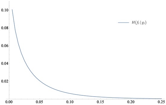
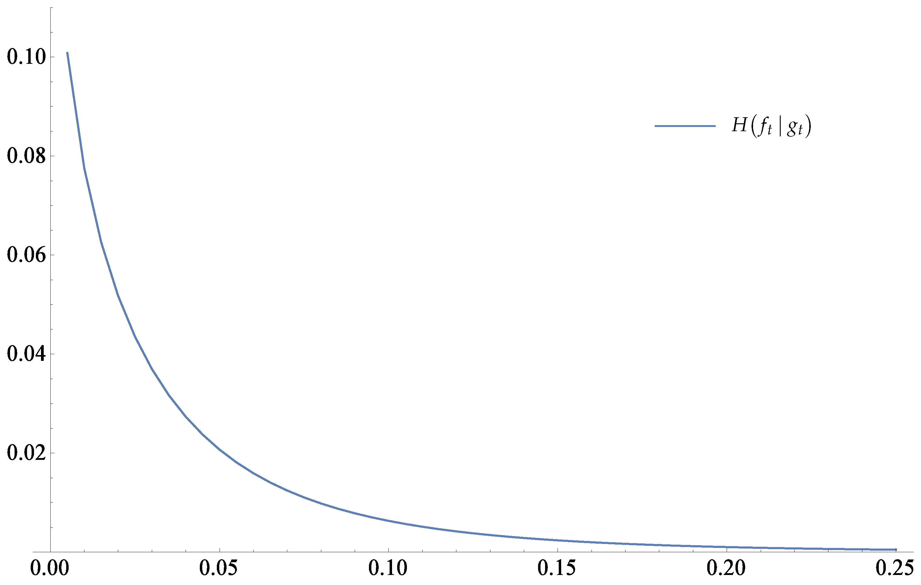
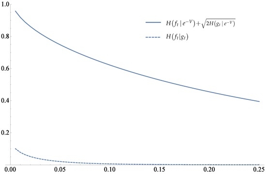
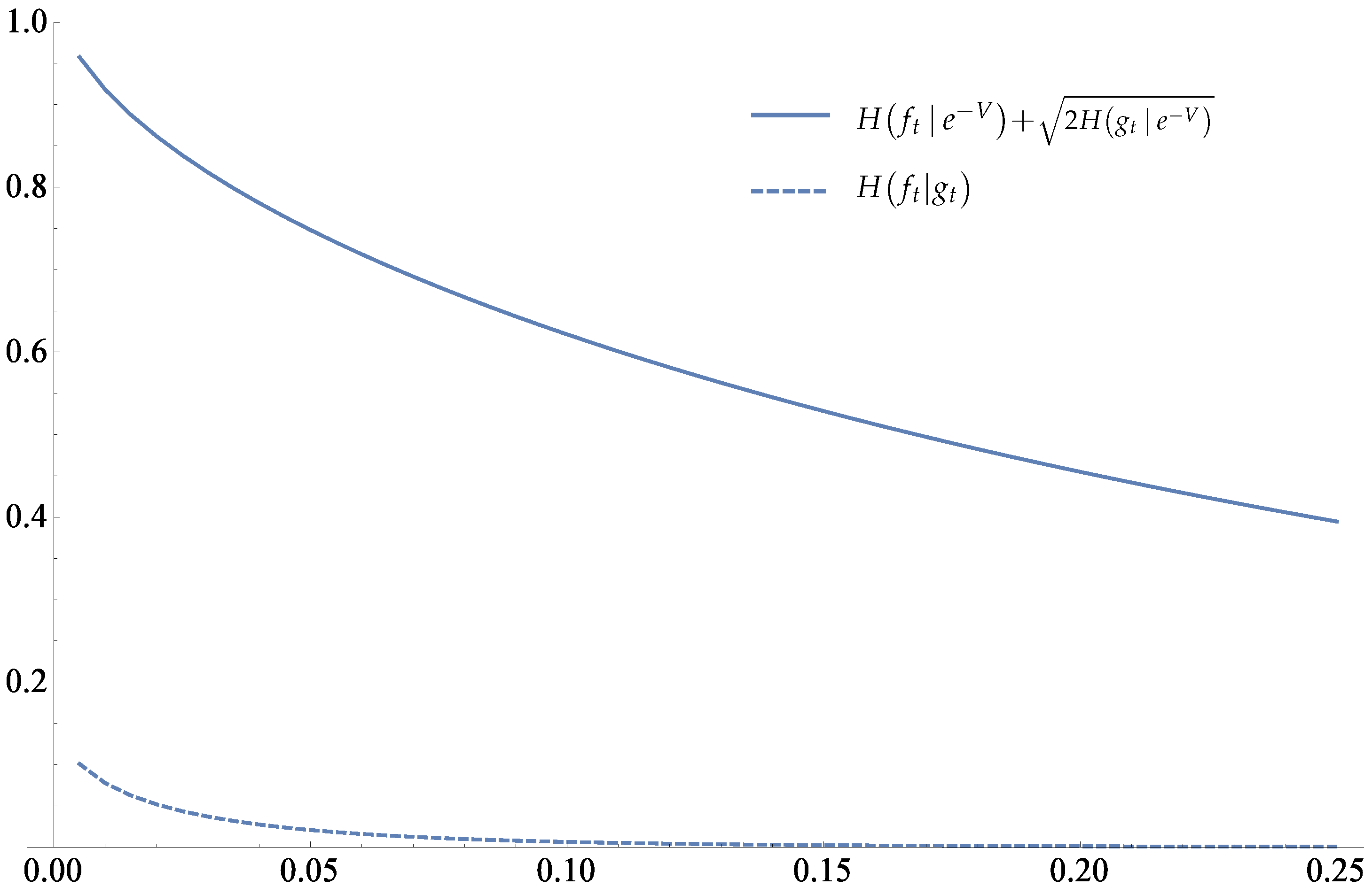
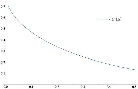
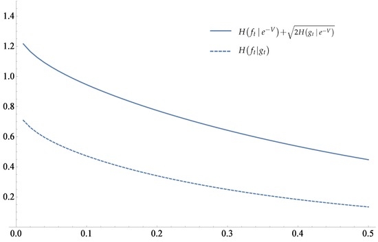
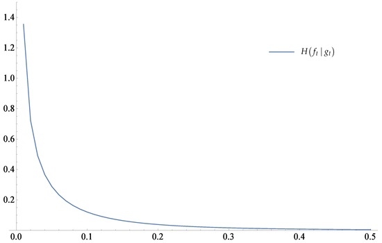
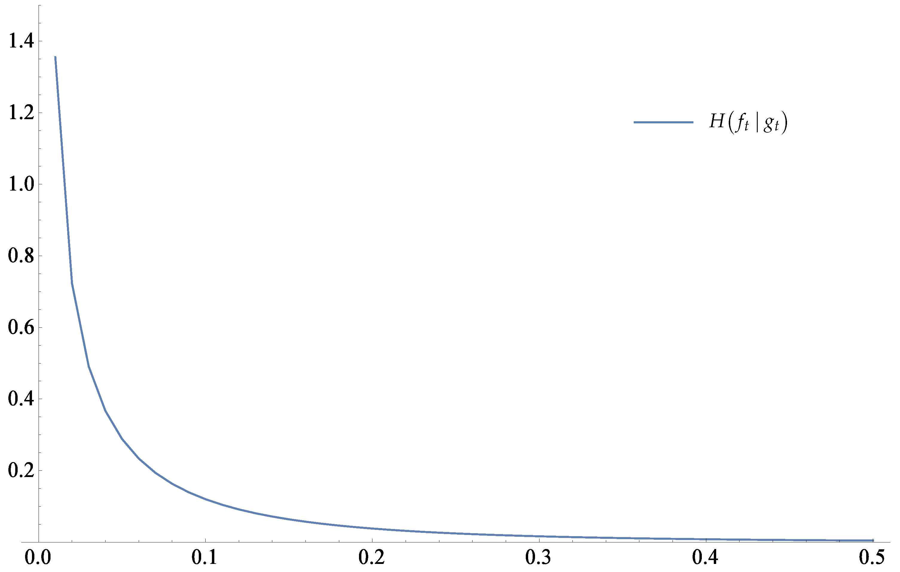
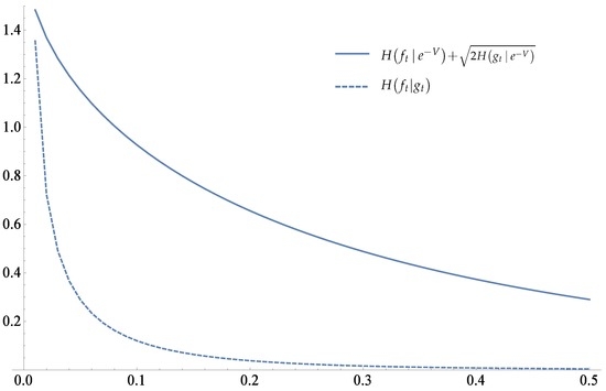
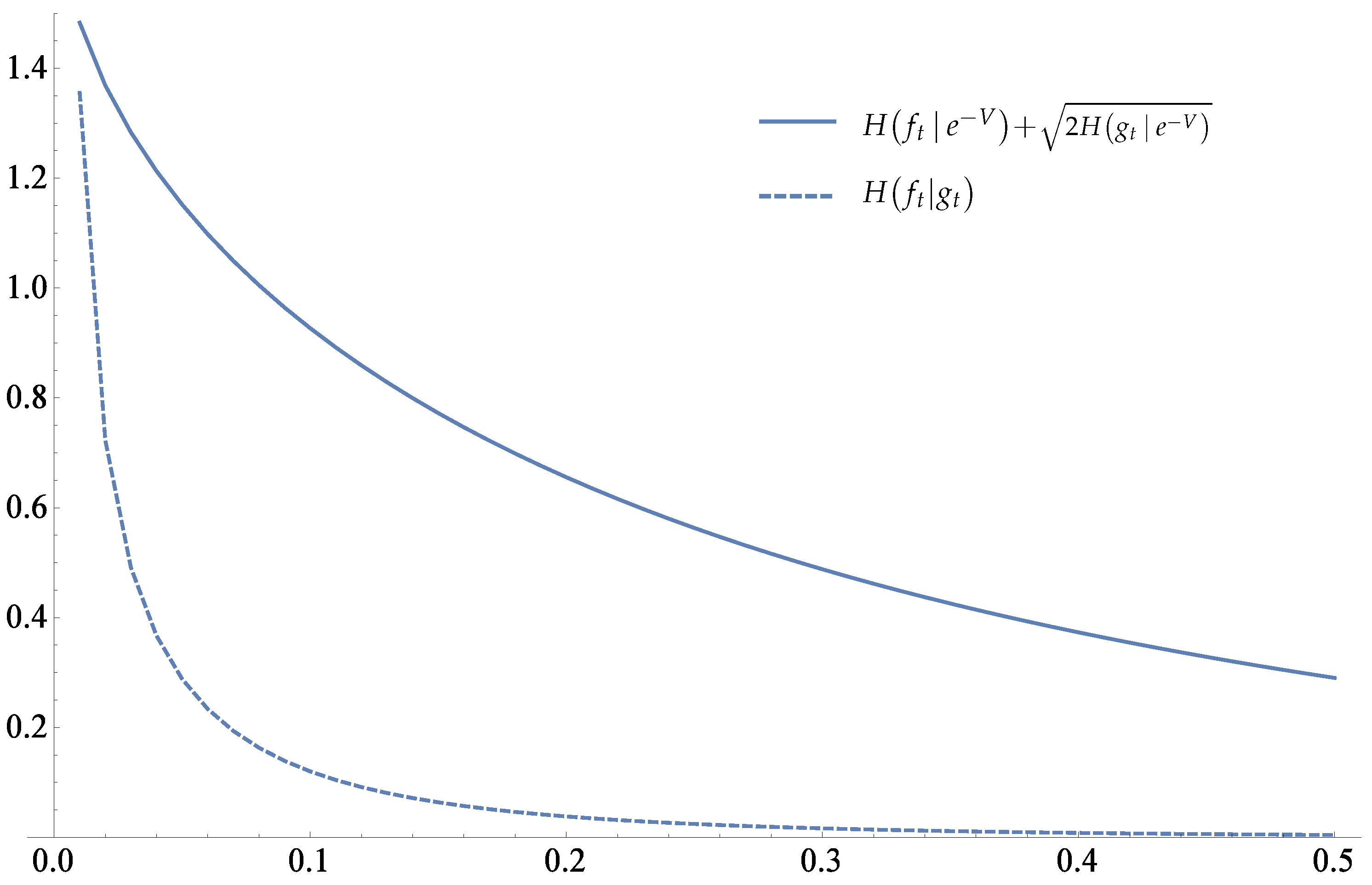
respectively. Now, we shall illustrate the convergence of $H\left(f_t|g_t\right)$ and the upper bound of the right-hand side in (47) numerically by graphs. We claim that the constant $\overline{M}$ can be assumed to be 1 because, in our assumptions (20), (21), and (22), the relative densities converge uniformly to 1. The convergence of $H\left(f_t|g_t\right)$ is illustrated in Figure 1.

Figure 1. The value of $H\left(f_t|g_t\right)$.

In Figure 2, the dashed curve indicates the convergence of $H\left(f_t|g_t\right)$ in Figure 1.

Figure 2. The value of $H\left(f_t|e^{-V}\right)+$ $\sqrt{2H\left(g_t|e^{-V}\right)}$.

Example 2.

In the second example, we put the initial reference measure as $g_0\left(x\right)=\phi (x,3)$, that is, we take the centered Gaussian of variance 3 as the initial reference measure, but $f_0\left(x\right)=u\left(x\right)$ is unchanged. In Figure 3, the convergence of $H\left(f_t|g_t\right)$ is illustrated.

Figure 3. The value of $H\left(f_t|g_t\right)$.

In Figure 4, the dashed curve indicates the convergence of $H\left(f_t|g_t\right)$ in Figure 3.

Figure 4. The value of $H\left(f_t|e^{-V}\right)+$ $\sqrt{2H\left(g_t|e^{-V}\right)}$.

Example 3.

In the third numerical example, the initial objective and the initial reference measures are given as the uniform distributions on the intervals $(-1,1)$ and $(-{\displaystyle \frac{1}{2}},{\displaystyle \frac{1}{2}})$, respectively. Namely, we set the densities as $f_0\left(x\right)=u\left(x\right)$ and $g_0=2u\left(2x\right)$. We illustrate the convergence of $H\left(f_t|g_t\right)$ in Figure 5.

Figure 5. The value of $H\left(f_t|g_t\right)$.

In Figure 6, the dashed curve indicates the convergence of $H\left(f_t|g_t\right)$ in Figure 5.

Figure 6. The value of $H\left(f_t|e^{-V}\right)+$ $\sqrt{2H\left(g_t|e^{-V}\right)}$.

5. Conclusions

The partial differential equation of Fokker–Planck describes the flow of the probability measures for diffusion process. The diffusion by the Fokker–Planck equation with the strictly convex potential V has the long-time asymptotic stationary measure $e^{-V}$. In the case of the relative entropy endowed with the stationary measure $e^{-V}$ as reference, the dissipation formula of the relative entropy of the diffusion flow by the Fokker–Planck equation with the potential V is known in literature.

In this paper, we have derived the similar dissipation formula under the more flexible situation. Namely, we have considered the situation that the reference measure is also evolved by the Fokker–Planck equation with the same potential function V for the objective measure. Then, we have obtained another integral representation of the relative entropy, which gives an extension of the formula of the entropy gap.

References

- Stam, A.J. Some inequalities satisfied by the quantities of information of Fisher and Shannon. Inf. Contr. 1959, 2, 101–112. [Google Scholar] [CrossRef]
- Barron, A. Entropy and the central limit theorem. Ann. Probab. 1986, 14, 336–342. [Google Scholar] [CrossRef]
- Villani, C. Topics in Optimal Transportation; American Mathematical: Providence, RI, USA, 2003. [Google Scholar]
- Verdú, S. Mismatched estimation and relative entropy. IEEE Trans. Inf. Theory 2010, 56, 3712–3719. [Google Scholar] [CrossRef]
- Hirata, M.; Nemoto, A.; Yoshida, H. An integral representation of the relative entropy. Entropy 2012, 14, 1469–1477. [Google Scholar] [CrossRef]
- Arnold, A.; Markowich, P.; Toscani, G.; Unterreiter, A. On convex Sobolev inequalities and the rate of convergence to equilibrium for Fokker–Planck type equations. Commum. Partial Differ. Equ. 2001, 26, 43–100. [Google Scholar] [CrossRef]
- Bakry, D.; Émery, M. Diffusions hypercontractives. In Séminar de Probabilités XIX; Springer: Berlin/Heidelberg, Germany, 1985; pp. 177–206. [Google Scholar]
- Otto, F.; Villani, C. Generalization of an inequality by Talagrand and links with the logarithmic Sobolev inequality. J. Funct. Anal. 2000, 173, 361–400. [Google Scholar] [CrossRef]
- Gross, L. Logarithmic Sobolev inequalities. Am. J. Math. 1975, 97, 1061–1083. [Google Scholar] [CrossRef]
- Carlen, E. Superadditivity of Fisher’s information and logarithmic Sobolev inequalities. J. Funct. Anal. 1991, 101, 194–211. [Google Scholar] [CrossRef]
- Talagrand, M. Transportation cost for Gaussian and other product measures. Geom. Funct. Anal. 1996, 6, 587–600. [Google Scholar] [CrossRef]
- Csiszar, I. Information-type measures of difference of probability distributions and indirect observations. Stud. Sci. Math. Hung. 1967, 2, 299–318. [Google Scholar]
- Csiszar, I.; Korner, J. Information Theory: Coding Theorems for Discrete Memoryless Systems, 2nd ed.; Cambridge University Press: Cambridge, UK, 2011. [Google Scholar]
- Yanomo, T. De Bruijn-type identity for systems with flux. Eur. J. Phys. B 2013, 86, 363. [Google Scholar] [CrossRef]
- Yanomo, T. Phase space gradient of dissipated work and information: A role of relative Fisher information. J. Math. Phys. 2013, 54, 113301. [Google Scholar] [CrossRef]
- Daffertshofer, A.; Plastino, A.R.; Plastino, A. Classical No-Cloning Theorem. Phys. Rev. Lett. 2002, 88, 210601. [Google Scholar] [CrossRef] [PubMed]
- Plastino, A.R.; Daffertshofer, A. Liouville Dynamics and the Conservation of Classical Information. Phys. Rev. Lett. 2004, 93, 138701. [Google Scholar] [CrossRef] [PubMed]
- Carlen, E.A.; Soffer, A. Entropy production by block variable summation and central limit theorems. Commun. Math. Phys. 1991, 140, 339–371. [Google Scholar] [CrossRef]
© 2016 by the author; licensee MDPI, Basel, Switzerland. This article is an open access article distributed under the terms and conditions of the Creative Commons Attribution (CC-BY) license (http://creativecommons.org/licenses/by/4.0/).