COVID-19 Outbreak Prediction with Machine Learning

Abstract

Several outbreak prediction models for COVID-19 are being used by officials around the world to make informed decisions and enforce relevant control measures. Among the standard models for COVID-19 global pandemic prediction, simple epidemiological and statistical models have received more attention by authorities, and these models are popular in the media. Due to a high level of uncertainty and lack of essential data, standard models have shown low accuracy for long-term prediction. Although the literature includes several attempts to address this issue, the essential generalization and robustness abilities of existing models need to be improved. This paper presents a comparative analysis of machine learning and soft computing models to predict the COVID-19 outbreak as an alternative to susceptible–infected–recovered (SIR) and susceptible-exposed-infectious-removed (SEIR) models. Among a wide range of machine learning models investigated, two models showed promising results (i.e., multi-layered perceptron, MLP; and adaptive network-based fuzzy inference system, ANFIS). Based on the results reported here, and due to the highly complex nature of the COVID-19 outbreak and variation in its behavior across nations, this study suggests machine learning as an effective tool to model the outbreak. This paper provides an initial benchmarking to demonstrate the potential of machine learning for future research. This paper further suggests that a genuine novelty in outbreak prediction can be realized by integrating machine learning and SEIR models.

1. Introduction

Access to accurate outbreak prediction models is essential to obtain insights into the likely spread and consequences of infectious diseases. Governments and other legislative bodies rely on insights from prediction models to suggest new policies and to assess the effectiveness of the enforced policies [1]. The novel coronavirus disease (COVID-19) has been reported to have infected more than 2 million people, with more than 132,000 confirmed deaths worldwide. The recent global COVID-19 pandemic has exhibited a nonlinear and complex nature [2]. In addition, the outbreak has differences with other recent outbreaks, which brings into question the ability of standard models to deliver accurate results [3]. In addition to the numerous known and unknown variables involved in the spread, the complexity of population-wide behavior in various geopolitical areas and differences in containment strategies dramatically increased model uncertainty [4]. Consequently, standard epidemiological models face new challenges to deliver more reliable results. To overcome this challenge, many novel models have emerged which introduce several assumptions to modeling (e.g., adding social distancing in the form of curfews, quarantines, etc.) [5,6,7].

To elaborate on the effectiveness of enforcing such assumptions, understanding standard dynamic epidemiological (e.g., susceptible-infected-recovered, SIR) models is essential [8]. The modeling strategy is formed around the assumption of transmitting the infectious disease through contacts, considering three different classes of well-mixed populations; susceptible to infection (class S), infected (class I), and the removed population (class R is devoted to those who have recovered, developed immunity, been isolated, or passed away). It is further assumed that the class I transmits the infection to class S where the number of probable transmissions is proportional to the total number of contacts [9,10,11]. The number of individuals in the class S progresses as a time series, often computed using a basic differential equation as follows (Equation (1)):

$$\frac{dS}{dt}=- \alpha SI$$

(1)

where $I$ is the infected population, and $S$ is the susceptible population, both as fractions. $\alpha$ represents the daily reproduction rate of the differential equation, regulating the number of susceptible infectious contacts. The value of $S$ in the time series produced by the differential equation gradually declines. Initially, it is assumed that at the early stage of the outbreak $S\approx 1$ while the number of individuals in class I is negligible. Thus, the increment $\frac{dI}{dt}$ becomes linear and the class I eventually can be computed as follows (Equation (2)):

$$\frac{dI}{dt}=\alpha SI-\beta I$$

(2)

where $\beta$ regulates the daily rate of new infections by quantifying the number of infected individuals competent in the transmission. Furthermore, the class R, representing individuals excluded from the spread of infection, is computed as follows:

$$\frac{dR}{dt}=\beta I$$

(3)

Under the unconstrained conditions of the excluded group, Equation (3), the outbreak exponential growth can be computed as follows (Equation (4)):

$$I \left(t\right)\approx I_{0 }exp\left\{(\alpha -\beta )\right\}$$

(4)

The outbreaks of a wide range of infectious diseases have been modeled using Equation (4). However, for the COVID-19 outbreak prediction, due to the strict measures enforced by authorities, the susceptibility to infection has been manipulated dramatically. For example, in China, Italy, France, Hungary, and Spain the SIR model cannot present promising results, as individuals committed voluntarily to quarantine and limited their social interaction. However, for countries where containment measures were delayed (e.g., United States) the model has shown relative accuracy [12]. Figure 1 shows the inaccuracy of conventional models applied to the outbreak in Italy by comparing the actual number of confirmed infections and epidemiological model predictions (this trend obviously depends on the approach chosen to model the outbreak; for example, the SEIR model performs usually better than SIR model). SEIR models, by considering the significant incubation period during which individuals are infected, showed increased model accuracy for the Varicella and Zika outbreaks [13,14]. SEIR models assume that the incubation period is a random variable and, similarly to the SIR model, there is a disease-free equilibrium [15,16]. It should be noted, however, that standard SIR and SEIR models will not fit well where the parameters related to social mixing and, thus, the contact network, are non-stationary through time [17]. A key cause of non-stationarity is where the social mixing (which determines the contact network) changes through time. Social mixing determines the reproductive number $R_0$, which is the number of susceptible individuals that an infected person will infect. When $R_0$ is less than 1 the epidemic will die out; when it is greater than 1 it will spread. $R_0$ for COVID-19 prior to lockdown was estimated as a massive 4 [1], representing a pandemic. It is expected that lockdown measures should bring $R_0$ down to less than 1. The key reason why SEIR models are difficult to fit for COVID-19 is non-stationarity of mixing, caused by nudging (step-by-step) intervention measures. A further drawback of conventional epidemiological models is the short lead time. To evaluate the performance of the models, the median success of the outbreak prediction presents useful information. The median prediction factor can be calculated as follows (Equation (5)):

$$f= \frac{Prediction}{True value}$$

(5)

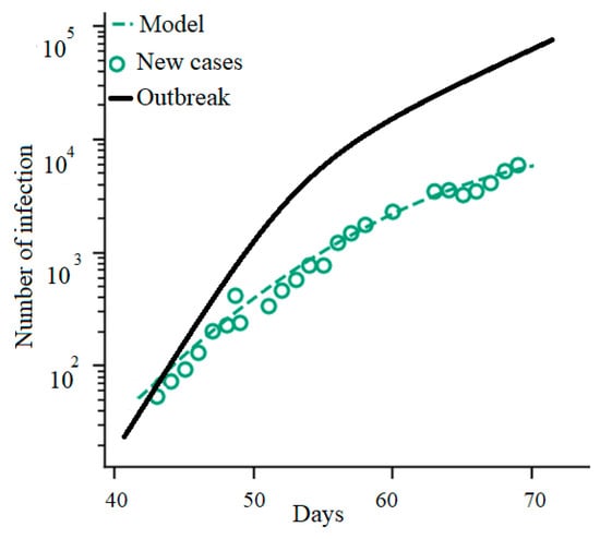
Figure 1. Italy’s COVID-19 outbreak: the actual number of confirmed infections vs. epidemiological model.

As the lead-time increases, the accuracy of the model declines. For instance, for the COVID-19 outbreak in Italy, the accuracy of the model for more than 5 days hence reduces from $f=1$ for the first five days to $f=0.86$ for day 6 [12]. Overall, the standard epidemiological models can be effective and reliable only if (a) the social interactions are stationary through time (i.e., no changes in interventions or control measures), and (b) there exists a great deal of knowledge of class R with which to compute Equation (3). To acquire information on class R, several novel models included data from social media or call data records (CDR), which showed promising results [18,19,20,21,22,23,24,25]. However, observation of the behavior of COVID-19 in several countries demonstrates a high degree of uncertainty and complexity [26]. Thus, for epidemiological models to be able to deliver reliable results, they must be adapted to the local situation based on insights into susceptibility to infection due to changes in public health interventions, and the various states in the SIR/SEIR model [27]. This imposes a huge limit on the generalization ability and robustness of conventional models. Advancing accurate models with a great generalization ability to be scalable to model both the regional and global pandemic is, thus, essential [28].

Due to the complexity and the large-scale nature of the problem in developing epidemiological models, machine learning (ML) has recently gained attention for building outbreak prediction models. ML approaches aim at developing models with higher generalization ability and greater prediction reliability for longer lead times [29,30,31,32,33].

Although ML methods were used in modeling former pandemics (e.g., Ebola, cholera, swine fever, H1N1 influenza, dengue fever, Zika, oyster norovirus [8,34,35,36,37,38,39,40,41,42,43]), there is a gap in the literature for peer-reviewed papers dedicated to COVID-19. Table 1 represents notable ML methods used for outbreak prediction. These ML methods are limited to the basic methods of random forest, neural networks, Bayesian networks, naïve Bayes, genetic programming, and classification and regression tree (CART). Although ML has long been established as a standard tool for modeling natural disasters and weather forecasting [44,45], its application in modeling outbreak is still in the early stages. More sophisticated ML methods (e.g., hybrids, ensembles) are yet to be explored. Consequently, the contribution of this paper is to explore the application of ML for modeling the COVID-19 pandemic. This paper aims to investigate the generalization ability of the proposed ML models and the accuracy of the proposed models for different lead times.

Table 1. Notable machine learning (ML) methods for outbreak prediction.

Authors	Journal	Outbreak Infection	Machine Learning
[39]	Transboundary and Emerging Diseases	Swine fever	Random Forest
[35]	Geospatial Health	Dengue fever	Neural Network
[42]	BMC Research Notes	Influenza	Random Forest
[41]	Journal of Public Health Medicine	Dengue/Aedes	Bayesian Network
[38]	Informatica	Dengue	LogitBoost
[8]	Global Ecology and Biogeography	H1N1 flu	Neural Network
[34]	Current Science	Dengue	Adopted multi-regression and Naïve Bayes
[36]	Environment International	Oyster norovirus	Neural Network
[37]	Water Research	Oyster norovirus	Genetic programming
[43]	Infectious Disease Modelling	Dengue	Classification and regression tree (CART)

The state-of-the-art machine learning methods for outbreak prediction modeling demonstrate two major research gaps for machine learning to address. Firstly, advancement in time-series prediction of outbreak and, secondly, improvement of SIR and SEIR models. Considering the drawbacks to the existing SIR and SEIR, machine learning can certainly contribute. This paper contributes to the advancement of time-series prediction of COVID-19. Consequently, an initial benchmarking is given to demonstrate the potential of machine learning for future research. The paper further suggests that a genuine novelty in outbreak prediction can be realized by integrating machine learning and SEIR models.

The remainder of this paper is organized as follows. Section 2 describes the methods and materials. The results are given in Section 3. Section 4 and Section 5 present the discussion and the conclusions, respectively.

2. Materials and Methods

Data were collected from worldometers website [46] for five countries, namely Italy, Germany, Iran, USA, and China, for total cases over 30 days. Figure 2 presents the total case number (cumulative statistic) for the considered countries. Currently, to contain the outbreak, the governments have implemented various measures to reduce transmission by inhibiting people’s movements and social activities. Although information on changes in social distancing is essential for advancing the epidemiological models, for modeling with machine learning no assumption is required. As can be seen in Figure 2, the growth rate in China was greater than that for Italy, Iran, Germany, and the USA in the early weeks of the disease [46].

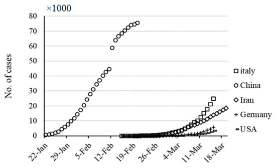
Figure 2. Cumulative number of cases for five countries during a thirty-day period.

The next step is to find the best model for the estimation of the time-series data. Logistic (Equation (6)), linear (Equation (7)), logarithmic (Equation (8)), quadratic (Equation (9)), cubic (Equation (10)), compound (Equation (11)), power (Equation (12)), and exponential (Equation (13)) equations were employed to develop the desired model. These models are generally not good fits for outbreak prediction beyond the available data. In this study, through parameter tuning we aim at finding the optimal performance of these models. The model with the best performance is later used for comparative analysis.

R = A/(1 + exp(((4*µ)*(L − x)/A) + 2))

(6)

R = Ax − B

(7)

R = A + Blog(x)

(8)

R = A + Bx + Cx²

(9)

R = A + Bx + Cx² + Dx³

(10)

R = AB^x

(11)

R = Ax^B

(12)

R = AEXP(Bx)

(13)

A, B, C, µ, and L are parameters (constants) that characterize the above-mentioned functions. These constants need to be estimated to develop an accurate estimation model. One of the goals of this study was to model time-series data based on the logistic microbial growth model. For this purpose, the modified equation of logistic regression was used to estimate and predict the prevalence (i.e., I/Population at a given time point) of disease as a function of time. Estimation of the parameters was performed using evolutionary algorithms such as the genetic algorithm (GA), particle swarm optimizer, and grey wolf optimizer. These algorithms are discussed in the following.

2.1. Evolutionary Algorithms

Evolutionary algorithms (EA) are powerful tools for solving optimization problems through intelligent methods. These algorithms are often inspired by natural processes to search for all possible answers as an optimization problem [47,48,49]. In the present study, the frequently used algorithms, (i.e., genetic algorithm (GA), particle swarm optimizer (PSO) and grey wolf optimizer (GWO)) were employed to estimate the parameters by solving a cost function.

2.1.1. Genetic Algorithm (GA)

GAs are considered a subset of “computational models” inspired by the concept of evolution [50]. These algorithms use “Potential Solutions”, “Candidate Solutions”, or “Possible Hypotheses” for a specific problem in a “chromosome-like” data structure. GA maintains vital information stored in these chromosome data structures by applying “Recombination Operators” to chromosome-like data structures [51,52,53,54]. In many cases, GAs are employed as “Function Optimizer” algorithms, which are algorithms used to optimize “Objective Functions”. Of course, the range of applications that use the GA to solve problems is very wide [53,55]. The implementation of the GA usually begins with the production of a population of chromosomes generated randomly, and bound up and down by the variables of the problem. In the next step, the generated data structures (chromosomes) are evaluated, and chromosomes that can better display the optimal solution of the problem are more likely to be used to produce new chromosomes. The degree of “goodness” of an answer is usually measured by the population of the current candidate’s answers [56,57,58,59,60]. The main algorithm of a GA process is demonstrated in Figure 3.

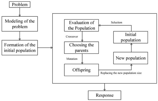
Figure 3. Genetic algorithm (GA).

In the present study, GA [60] was employed for estimation of the parameters of Equations (6) to (13). The population number was selected to be 300 and the maximum generation (as iteration number) was determined to be 500 according to different trial and error processes to reduce the cost function value. The cost function was defined as the mean square error between the target and estimated values according to Equation (14):

$$MSE=\sqrt{\frac{{\left(Es-T\right)}^2}{N}}$$

(14)

where Es refers to estimated values, T refers to the target values, and N refers to the number of data.

2.1.2. Particle Swarm Optimization (PSO)

In 1995, Kennedy and Eberhart [60] introduced the PSO as an uncertain search method for optimization purposes. The algorithm was inspired by the mass movement of birds looking for food. A group of birds accidentally look for food in a space. There is only one piece of food in the search space. Each solution in PSO is called a particle, which is equivalent to a bird in the bird’s mass movement algorithm. Each particle has a value that is calculated by a competency function which increases as the particle in the search space approaches the target (food in the bird’s movement model). Each particle also has a velocity that guides the motion of the particle. Each particle continues to move in the problem space by tracking the optimal particles in the current state [61,62,63]. The PSO method is rooted in Reynolds’ work, which is an early simulation of the social behavior of birds. The mass of particles in nature represents collective intelligence. Consider the collective movement of fish in water or birds during migration. All members move in perfect harmony with each other, hunt together if they are to be hunted, and escape from the clutches of a predator by moving toward other prey if they are preyed upon [64,65,66]. Particle properties in this algorithm include [66,67,68]:

• Each particle independently looks for the optimal point.
• Each particle moves at the same speed at each step.
• Each particle remembers its best position in the space.
• The particles work together to inform each other of the places they are looking for.
• Each particle is in contact with its neighboring particles.
• Every particle is aware of the particles that are in the neighborhood.
• Every particle is known as one of the best particles in its neighborhood.

The PSO implementation steps can be summarized as: the first step establishes and evaluates the primary population. The second step determines the best personal memories and the best collective memories. The third step updates the speed and position. If the conditions for stopping are not met, the cycle will return to the second step.

The PSO algorithm is a population-based algorithm [69,70]. This property makes it less likely to be trapped in a local minimum. This algorithm operates according to possible rules, not definite rules. Therefore, PSO is a random optimization algorithm that can search for unspecified and complex areas. This makes PSO more flexible and durable than conventional methods. PSO deals with non-differential target functions because the PSO uses the information result (performance index or target function to guide the search in the problem area). The quality of the proposed route response does not depend on the initial population. Starting from anywhere in the search space, the algorithm ultimately converges on the optimal answer. PSO has great flexibility to control the balance between the local and overall search space. This unique PSO property overcomes the problem of improper convergence and increases the search capacity. All of these features make PSO different from the GA and other innovative algorithms [62,66,68].

In the present study, PSO was employed for estimation of the parameters of Equations (6) to (13). The population number was selected to be 1000 and the iteration number was determined to be 500 according to different trial and error processes to reduce the cost function value. The cost function was defined as the mean square error between the target and estimated values according to Equation (14).

2.1.3. Grey Wolf Optimizer (GWO)

One recently developed smart optimization algorithm that has attracted the attention of many researchers is the grey wolf algorithm. Like most other intelligent algorithms, GWO is inspired by nature. The main idea of the grey wolf algorithm is based on the leadership hierarchy in wolf groups and how they hunt [71]. In general, there are four categories of wolves among the herd of grey wolves, alpha, beta, delta and omega. Alpha wolves are at the top of the herd’s leadership pyramid; the remainder of the wolves take orders from the alpha group and follow them (usually there is only one alpha wolf in each herd). Beta wolves are in the lower tier, but their superiority over delta and omega wolves allows them to provide advice and help to alpha wolves. Beta wolves are responsible for regulating and orienting the herd based on alpha movement. Delta wolves, which are next in line in the power pyramid of the wolf herd, are usually made up of guards, elderly population, caregivers of damaged wolves, and so on. Omega wolves are the weakest in the power hierarchy [71]. Equations (15) to (18) are used to model the hunting tool:

$$\overrightarrow{D}=|\overrightarrow{C},\overrightarrow{X_p}\left(t\right)-\overrightarrow{X_{ }}\left(t\right)|$$

(15)

$$\overrightarrow{X}\left(t+1\right)=\overrightarrow{X_p}\left(t\right)-\overrightarrow{A},\overrightarrow{D}$$

(16)

$$\overrightarrow{X}\left(t+1\right)=\overrightarrow{X_p}\left(t\right)-\overrightarrow{A},\overrightarrow{D}$$

(17)

$$\overrightarrow{C}=2\overrightarrow{r_2}$$

(18)

where t represents repetition of the algorithm. $\overrightarrow{A}$ and $\overrightarrow{C}$ are vectors of the prey site and the $\overrightarrow{X}$ vectors represent the locations of the grey wolves. $\overrightarrow{a}$ is linearly reduced from 2 to 0 during the repetition. $\overrightarrow{r_1}$ and $\overrightarrow{r_2}$ are random vectors in which each element can take on realizations in the range [0,1]. The GWO algorithm flowchart is shown in Figure 4.

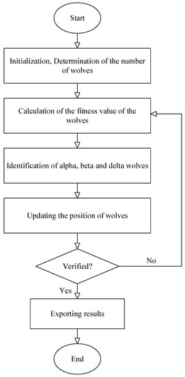
Figure 4. Grey wolf optimizer (GWO) algorithm.

In the present study, GWO [71] was employed for estimation of the parameters of Equations (1) to (8). The population number was selected to be 500 and the iteration number was determined to be 1000 according to different trial and error processes to reduce the cost function value. The cost function was defined as the mean square error between the target and estimated values according to Equation (14).

2.2. Machine Learning (ML)

ML is regarded as a subset of Artificial Intelligence (AI). Using ML techniques, the computer learns to use patterns or “training samples” in data (processed information) to predict or make intelligent decisions without overt planning [72,73]. In other words, ML is the scientific study of algorithms and statistical models used by computer systems that use patterns and inference to perform tasks instead of using explicit instructions [74,75].

Time series are data sequences collected over a period of time [76], which can be used as inputs to ML algorithms. This type of data reflects the changes that a phenomenon has undergone over time. Let X^t be a time-series vector, in which x_t is the outbreak at time point t and T is the set of all equidistant time points. To train ML methods effectively, we defined two scenarios, listed in Table 2.

Table 2. Input and output variables for training ML methods by time-series data.

	Inputs	Input Number	Output
Scenario 1	xt−1, xt−7, xt−14, and xt−21	Four inputs	xt (outbreak)
Scenario 2	xt−1, xt−2, xt−3, xt−4, and xt−5	Five inputs	xt (outbreak)

As can be seen in Table 2, scenario 1 employs data for three weeks to predict the outbreak on day t and scenario 2 employs outbreak data for five days to predict the outbreak for day t. Both of these scenarios were employed for fitting the ML methods. In the present research, two frequently used ML methods, the multi-layered perceptron (MLP) and adaptive network-based fuzzy inference system (ANFIS), were employed for the prediction of the outbreak in the five countries.

2.2.1. Multi-Layered Perceptron (MLP)

The Artificial Neural Network (ANN) is an idea inspired by the biological nervous system, which processes information in the same way as the brain. The key element of this idea is the new structure of the information processing system [77,78,79]. The system is made up of several highly interconnected processing elements called neurons that work together to solve a problem [79,80]. ANNs, like humans, learn by example. The neural network is set up during a learning process to perform specific tasks, such as identifying patterns and categorizing information. In biological systems, learning is regulated by the synaptic connections between nerves. This method is also used in neural networks [81]. By processing experimental data, ANNs transfer knowledge or a law behind the data to the network structure, which is called learning. Basically, learning ability is the most important feature of such a smart system. A learning system is more flexible and easier to plan, so it can better respond to new issues and changes in processes [82].

In ANNs, with the help of programming knowledge, a data structure is designed that can act like a neuron. This data structure is called a node [83,84]. In this structure, the network between these nodes is trained by applying an educational algorithm to it. In this memory or neural network, the nodes have two active states (on or off) and one inactive state (off or 0), and each edge (synapse or connection between nodes) has a weight. Positive weights stimulate or activate the next inactive node, and negative weights inactivate or inhibit the next connected node (if active) [79,85]. In the ANN architecture, for the neural cell c, the input b_p enters the cell from the previous cell p (Equation (19)). w_pc is the weight of the input b_p with respect to cell c and a_c is the sum of the multiplications of the inputs and their weights [86]:

$$a_c={\displaystyle \sum }{w}_{pc}{b}_{pc}$$

(19)

A non-linear function θ_c is applied to a_c. Accordingly, b_c can be calculated as Equation (20) [85]:

$$b_c={\theta }_c\left(a_c\right)$$

(20)

Similarly, w_cn is the weight of the b_cn which is the output of c to n. W is the collection of all of the weights of the neural network in a set. For input x and output y, h_w(x) is the output of the neural network. The main goal is to learn these weights to reduce the error values between y and h_w(x). That is, the goal is to minimize the cost function Q(W), Equation (21) [86]:

$$Q\left(W\right)=\frac{1}{2}{\displaystyle \sum }_{i=1}^n{\left(y_i-o_i\right)}^2$$

(21)

In the present research, one of the frequently used types of ANN called the MLP [77] was employed to predict the outbreak. The MLP was trained using a dataset related to both scenarios. For the training of the network, 8, 12, and 16 inner neurons were tried to achieve the best response. Results were evaluated by root mean square error (RMSE) and correlation coefficient to reduce the cost function value. Figure 5 presents the architecture of the MLP.

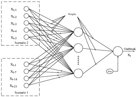
Figure 5. Architecture of the multi-layered perceptron (MLP).

2.2.2. Adaptive Neuro Fuzzy Inference System (ANFIS)

An adaptive neuro fuzzy inference system is a type of ANN based on the Takagi–Sugeno fuzzy system [87]. This approach was developed in the early 1990s. Because this system integrates the concepts of neural networks and fuzzy logic, it can take advantage of both capabilities in a unified framework. This technique is one of the most frequently used and robust hybrid ML techniques. It is consistent with a set of fuzzy if–then rules that can be learned to approximate nonlinear functions [88,89]. Hence, ANFIS was proposed as a universal estimator. An important element of fuzzy systems is the fuzzy partition of the input space [90,91]. For input k, the fuzzy rules in the input space make a k-faced fuzzy cube. Achieving a flexible partition for nonlinear inversion is non-trivial. The idea of this model is to build a neural network whose outputs are a degree of the input that belongs to each class [92,93,94]. The membership functions (MFs) of this model can be nonlinear, multidimensional and, thus, different to conventional fuzzy systems [95,96,97]. In ANFIS, neural networks are used to increase the efficiency of fuzzy systems. The method used to design neural networks is to employ fuzzy systems or fuzzy-based structures. This model is a kind of division and conquest method. Instead of using one neural network for all the input and output data, several networks are created in this model:

• A fuzzy separator to cluster input–output data within multiple classes.
• A neural network for each class.
• Training neural networks with output–input data in the corresponding classes.

Figure 6 presents a simple architecture for ANFIS.

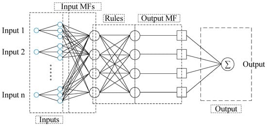
Figure 6. Adaptive neuro fuzzy inference system (ANFIS) architecture.

In the present study, ANFIS is developed to tackle two scenarios described in Table 2. Each input included by two MFs with the Tri shape, Trap shape, and Gauss shape MFs. The output MF type was selected to be linear with a hybrid optimizer type.

2.2.3. Evaluation Criteria

Evaluation was conducted using the root mean square error (RMSE) (Equation (22)) and correlation coefficient (Equation (23)). These statistics compare the target and output values, and calculate a score as an index for the performance and accuracy of the developed methods [88,98]. Presents the evaluation criteria equations.

$$\mathrm{Correlation} \mathrm{coefficient}= \frac{N\sum {(AP)}^{ }-\sum {(A)}^{ }\sum {(P)}^{ }}{\sqrt{[N\sum A^2-{(\sum A)}^{ }{}^2][N\sum P^2-{(\sum AP)}^{ }{}^2] }}$$

(22)

$$\mathrm{RMSE}= \sqrt{\frac{1}{N}\sum \hspace{1em}{(A-P)}^2}$$

(23)

where N is the number of data, and P and A are, respectively, the predicted (output) and desired (target) values.

3. Results

Table 3, Table 4, Table 5, Table 6, Table 7, Table 8, Table 9 and Table 10 present the results of the accuracy statistics for the logistic, linear, logarithmic, quadratic, cubic, compound, power, and exponential equations, respectively. The coefficients of each equation were calculated by the three ML optimizers; GA, PSO, and GWO. The table contains country name, model name, population size, number of iterations, processing time, RMSE, and correlation coefficient.

Table 3. Accuracy statistics for the logistic model.

Country	Model	Pop. Size	Iteration	Processing Time	RMSE	Correlation Coefficient
Italy	GA	300	500	82 s	1028.98	0.996
	PSO	1000	500	36 s	3358.1	0.997
	GWO	500	1000	14 s	187.15	0.999
China	GA	300	500	79 s	42,160.4	0.982
	PSO	1000	500	35 s	2524.44	0.994
	GWO	500	1000	13 s	2270.58	0.995
Iran	GA	300	500	81 s	1267.04	0.992
	PSO	1000	500	36 s	628.62	0.997
	GWO	500	1000	13 s	392.88	0.996
USA	GA	300	500	82 s	1028.98	0.999
	PSO	1000	500	38 s	350.33	0.999
	GWO	500	1000	15 s	22.35	0.999
Germany	GA	300	500	86 s	5339.5	0.983
	PSO	1000	500	39 s	555.32	0.997
	GWO	500	1000	16 s	55.54	0.999

Table 4. Accuracy statistics for the linear model.

Country	Model	Pop. Size	Iteration	Processing Time	RMSE	Correlation Coefficient
Italy	GA	300	500	92 s	3774.06	0.845
	PSO	1000	500	42 s	3645.76	0.844
	GWO	500	1000	16 s	3642.44	0.844
China	GA	300	500	91 s	7188.95	0.981
	PSO	1000	500	39 s	6644.16	0.982
	GWO	500	1000	14 s	5039.48	0.982
Iran	GA	300	500	96 s	3330.45	0.943
	PSO	1000	500	45 s	2072.71	0.944
	GWO	500	1000	18 s	1981.97	0.944
USA	GA	300	500	88 s	850.22	0.745
	PSO	1000	500	40 s	596.69	0.746
	GWO	500	1000	17 s	592.48	0.746
Germany	GA	300	500	93 s	1118.77	0.758
	PSO	1000	500	47 s	964.46	0.759
	GWO	500	1000	20 s	951.63	0.759

Table 5. Accuracy statistics for the logarithmic model.

	Model	Pop. Size	Iteration	Processing Time	RMSE	Correlation Coefficient
Italy	GA	300	500	98 s	8325.33	0.634
	PSO	1000	500	51 s	8818.2	0.634
	GWO	500	1000	20 s	9296.59	0.634
China	GA	300	500	96 s	40,828.2	0.847
	PSO	1000	500	42 s	43,835.37	0.847
	GWO	500	1000	17 s	42,714.93	0.847
Iran	GA	300	500	102 s	4929.97	0.757
	PSO	1000	500	59 s	8775.56	0.757
	GWO	500	1000	22 s	8995.52	0.756
USA	GA	300	500	94 s	889.15	0.538
	PSO	1000	500	37 s	1130.33	0.538
	GWO	500	1000	15 s	1135.12	0.538
Germany	GA	300	500	95 s	1552.22	0.548
	PSO	1000	500	45 s	1966.81	0.548
	GWO	500	1000	21 s	1878.67	0.548

Table 6. Accuracy statistics for the quadratic model.

	Model	Pop. Size	Iteration	Processing Time	RMSE	Correlation Coefficient
Italy	GA	300	500	102 s	6710.01	0.976
	PSO	1000	500	54 s	5102.4	0.953
	GWO	500	1000	26 s	1272.1	0.982
China	GA	300	500	100 s	7921.33	0.992
	PSO	1000	500	46 s	4328.71	0.993
	GWO	500	1000	20 s	3710.16	0.993
Iran	GA	300	500	105 s	6771.74	0.995
	PSO	1000	500	62 s	822.09	0.998
	GWO	500	1000	24 s	310.02	0.998
USA	GA	300	500	98 s	754.6	0.931
	PSO	1000	500	38 s	791.92	0.853
	GWO	500	1000	19 s	307.58	0.938
Germany	GA	300	500	101 s	7577	0.904
	PSO	1000	500	49 s	752.95	0.923
	GWO	500	1000	26 s	472.62	0.946

Table 7. Accuracy statistics for the cubic model.

	Model	Pop. Size	Iteration	Processing Time	RMSE	Correlation Coefficient
Italy	GA	300	500	112 s	7973.11	0.993
	PSO	1000	500	61 s	4827.08	0.996
	GWO	500	1000	34 s	324.33	0.998
China	GA	300	500	113 s	15,697.84	0.971
	PSO	1000	500	59 s	3611.15	0.995
	GWO	500	1000	34 s	2429.45	0.995
Iran	GA	300	500	120 s	5852.66	0.995
	PSO	1000	500	88 s	3809.76	0.997
	GWO	500	1000	39 s	250.2	0.999
USA	GA	300	500	110 s	37,766.56	0.875
	PSO	1000	500	49 s	678.36	0.979
	GWO	500	1000	25 s	118.24	0.991
Germany	GA	300	500	116 s	1709.06	0.744
	PSO	1000	500	59 s	1812.78	0.967
	GWO	500	1000	29 s	196.8	0.99

Table 8. Accuracy statistics for the compound model.

	Model	Pop. Size	Iteration	Processing Time	RMSE	Correlation Coefficient
Italy	GA	300	500	92 s	8347.51	0.912
	PSO	1000	500	53 s	195,705.52	0.918
	GWO	500	1000	22 s	12,585.79	0.951
China	GA	300	500	90 s	41,544.05	0.986
	PSO	1000	500	48 s	40,195.9	0.988
	GWO	500	1000	23 s	24,987.34	0.895
Iran	GA	300	500	99 s	1,487,501.93	0.782
	PSO	1000	500	81 s	8216.81	0.986
	GWO	500	1000	26 s	13,635.01	0.864
USA	GA	300	500	96 s	655.62	0.994
	PSO	1000	500	32 s	1026.03	0.827
	GWO	500	1000	16 s	364.87	0.988
Germany	GA	300	500	98 s	15,333,537.7	0.93
	PSO	1000	500	72 s	1557.23	0.976
	GWO	500	1000	20 s	431.97	0.998

Table 9. Accuracy statistics for the power model.

	Model	Pop. Size	Iteration	Processing Time	RMSE	Correlation Coefficient
Italy	GA	300	500	72 s	7063.4	0.983
	PSO	1000	500	40 s	6150.52	0.982
	GWO	500	1000	13 s	3450.96	0.991
China	GA	300	500	65 s	39,669.92	0.976
	PSO	1000	500	39 s	19,365.58	0.987
	GWO	500	1000	12 s	4078.99	0.989
Iran	GA	300	500	83 s	2,343,032.5	0.951
	PSO	1000	500	65 s	92,755.53	0.975
	GWO	500	1000	15 s	1031.6	0.991
USA	GA	300	500	79 s	1030.01	0.779
	PSO	1000	500	24 s	1005.27	0.751
	GWO	500	1000	11 s	790.16	0.837
Germany	GA	300	500	85 s	1475.39	0.871
	PSO	1000	500	69 s	1387.94	0.916
	GWO	500	1000	14 s	1341.91	0.875

Table 10. Accuracy statistics for the exponential model.

	Model	POP. SIZE	Iteration	Processing Time	RMSE	Correlation Coefficient
Italy	GA	300	500	79 s	8163.1	0.995
	PSO	1000	500	48 s	52,075,925.37	0.839
	GWO	500	1000	18 s	12,585.79	0.951
China	GA	300	500	71 s	68,991.73	0.866
	PSO	1000	500	45 s	80,104.27	0.865
	GWO	500	1000	17 s	24,987.34	0.895
Iran	GA	300	500	89 s	1,436,025.84	0.767
	PSO	1000	500	70 s	3,745,673.26	0.744
	GWO	500	1000	21 s	13,635.01	0.864
USA	GA	300	500	84 s	457,051.4	0.974
	PSO	1000	500	30 s	982.37	0.932
	GWO	500	1000	15 s	364.87	0.988
Germany	GA	300	500	87 s	8176.54	0.981
	PSO	1000	500	74 s	3278.55	0.998
	GWO	500	1000	19 s	431.97	0.998

According to Table 3, Table 4, Table 5, Table 6, Table 7, Table 8, Table 9 and Table 10, GWO provided the highest accuracy (smallest RMSE and largest correlation coefficient) and smallest processing time compared to PSO and GA for fitting the logistic, linear, logarithmic, quadratic, cubic, power, compound, and exponential equations for all five countries. It can be suggested that GWO is a sustainable optimizer due to its acceptable processing time compared with PSO and GA. Therefore, GWO was selected as the best optimizer by providing the highest accuracy values compared with PSO and GA. In general, it can be claimed that GWO, by suggesting the best parameter values for the functions presented in Equations (6)–(13), increases outbreak prediction accuracy for COVID-19 in comparison with PSO and GA. Therefore, the functions derived by GWO were selected as the best predictors for this research.

Table 11, Table 12, Table 13, Table 14 and Table 15 present the description and coefficients of the linear, logarithmic, quadratic, cubic, compound, power, exponential, and logistic equations estimated by GWO. Table 11, Table 12, Table 13, Table 14 and Table 15 also present the RMSE and r-square values for each equation fitted to data for China, Italy, Iran, Germany, and USA, respectively.

Table 11. Model description for China fitted by GWO.

Model Name	Description	RMSE	r-Square
Linear	$\mathrm{R}=3036.4\times \mathrm{x}-13509.84$	5039.48	0.964
Logarithmic	$\mathrm{R}=-33948.15+27124.70\times \log \left(\mathrm{x}\right)$	42,714.93	0.718
Quadratic	$\mathrm{R}=-5080.88+1455.98\times \mathrm{x}+50.98\times {\mathrm{x}}^2$	3710.16	0.98
Cubic	$\mathrm{R}=3984.73-1790.2\times \mathrm{x}+308.52\times {\mathrm{x}}^2-5.53\times {\mathrm{x}}^3$	2429.45	0.99
Compound	$\mathrm{R}=1601.03\times {1.16}^{\mathrm{x}}$	24,987.34	0.801
Power	$\mathrm{R}=262.27\times {\mathrm{x}}^{1.69}$	4078.99	0.98
Exponential	$\mathrm{R}=1601.03\times \mathrm{EXP}\left(0.15\times \mathrm{x}\right)$	24,987.34	0.801
Logistic	$\mathrm{R}=85011.297/\left(1+\mathrm{EXP}\left(\left(\left(4\times 4483.304\right)\ast \left(9.423-\mathrm{x}\right)/85011.297\right)+2\right)\right)$	2270.58	0.992

Table 12. Model description for Italy fitted by GWO.

Model Name	Description	RMSE	r-Square
Linear	$\mathrm{R}=663.71\times \mathrm{x}-5437.25$	3642.44	0.713
Logarithmic	$\mathrm{R}=-7997.93+5162.83\times \log \left(\mathrm{x}\right)$	9296.59	0.402
Quadratic	$\mathrm{R}=2998.21-917.93\times \mathrm{x}+51.02\times {\mathrm{x}}^2$	1272.1	0.965
Cubic	$\mathrm{R}=-978.55+506.05\times \mathrm{B}2-61.95\times {\mathrm{x}}^2+2.42\times {\mathrm{x}}^3$	324.33	0.997
Compound	$\mathrm{R}=2.78\times {1.406}^{\mathrm{x}}$	12,585.79	0.904
Power	$\mathrm{R}=0.096\times {\mathrm{x}}^{3.476}$	3450.96	0.984
Exponential	$\mathrm{R}=2.786\times \mathrm{EXP}\left(0.341\times \mathrm{x}\right)$	12,585.79	0.904
Logistic	$\mathrm{R}=70731.084/\left(1+\mathrm{EXP}\left(\left(\left(4\times 3962.88\right)\times \left(23.88-\mathrm{x}\right)/70731.08\right)+2\right)\right)$	187.15	0.999

Table 13. Model description for Iran fitted by GWO.

Model Name	Description	RMSE	r-Square
Linear	$\mathrm{R}=656.068\times \mathrm{x}-4527.69$	1981.97	0.891
Logarithmic	$\mathrm{R}=-7921.009+5449.784\times \log \left(\mathrm{x}\right)$	8995.52	0.574
Quadratic	$\mathrm{R}=310.48-251.09\times \mathrm{x}+29.26\times {\mathrm{x}}^2$	310.027	0.997
Cubic	$\mathrm{R}=902.33-463.02\times \mathrm{x}+46.07\times {\mathrm{x}}^2-0.36\times {\mathrm{x}}^3$	250.204	0.998
Compound	$\mathrm{R}=13.26\times {1.33}^{\mathrm{x}}$	13,635.014	0.748
Power	$\mathrm{R}=0.51\times {\mathrm{x}}^{3.09}$	1031.607	0.982
Exponential	$\mathrm{R}=13.26\times \mathrm{EXP}\left(0.28\times \mathrm{x}\right)$	13,635.014	0.748
Logistic	$\mathrm{R}=21936.052/\left(1+\mathrm{EXP}\left(\left(\left(4\ast 1255.36\right)\times \left(14.66-\mathrm{x}\right)/21936.052\right)+2\right)\right)$	392.88	0.996

Table 14. Model description for Germany fitted by GWO.

Model Name	Description	RMSE	r-Square
Linear	$\mathrm{R}=128.421\times \mathrm{x}-1130.294$	951.635	0.577
Logarithmic	$\mathrm{R}=-1528.684+959.941\times \log \left(\mathrm{x}\right)$	1878.672	0.3
Quadratic	$\mathrm{R}=911.113-254.342\times \mathrm{x}+12.347\times {\mathrm{x}}^2$	472.624	0.895
Cubic	$\mathrm{R}=-478.087+243.097\times \mathrm{x}-27.118\times {\mathrm{x}}^2+0.848\times {\mathrm{x}}^3$	196.809	0.981
Compound	$\mathrm{R}=3.821\times {1.263}^{\mathrm{x}}$	431.975	0.996
Power	$\mathrm{R}=0.937{\mathrm{x}}^{2.021}$	1341.911	0.766
Exponential	$\mathrm{R}=3.821\times \mathrm{EXP}\left(0.233\times \mathrm{x}\right)$	431.975	0.996
Logistic	$\mathrm{R}=55179.669/\left(1+\mathrm{EXP}\left(\left(\left(4\times 3740.457\right)\times \left(30.49-\mathrm{x}\right)/55179.669\right)+2\right)\right)$	55.546	0.998

Table 15. Model description for USA fitted by GWO.

Model Name	Description	RMSE	r-Square
Linear	$\mathrm{R}=76.833\times \mathrm{x}-666.79$	592.486	0.557
Logarithmic	$\mathrm{R}=-902.637+573.32\times \log \left(\mathrm{x}\right)$	1135.124	0.289
Quadratic	$\mathrm{R}=584.76-157.831\times \mathrm{x}+7.569\times {\mathrm{x}}^2$	307.585	0.88
Cubic	$\mathrm{R}=-333.235+170.881\times \mathrm{x}-18.509\times {\mathrm{x}}^2+0.56\times {\mathrm{x}}^3$	118.247	0.982
Compound	$\mathrm{R}=6.296\times {1.214}^{\mathrm{x}}$	364.875	0.977
Power	$\mathrm{R}=1.707\times {\mathrm{x}}^{1.735}$	790.163	0.702
Exponential	$\mathrm{R}=6.296\times \mathrm{EXP}\left(0.194\times \mathrm{x}\right)$	364.875	0.977
Logistic	$\mathrm{R}=32604.552/\left(1+\mathrm{EXP}\left(\left(\left(4\times 2288.932\right)\times \left(30.303-\mathrm{x}\right)/32604.552\right)+2\right)\right)$	22.354	0.999

As is clear from Table 11, Table 12, Table 13, Table 14 and Table 15, in general, the logistic equation followed by the quadratic and cubic equations provided the smallest RMSE and the largest r-square values for the prediction of COVID-19 outbreak. The claim can also be considered from Figure 7, Figure 8, Figure 9, Figure 10 and Figure 11, which present the capability and trend of each model derived by GWO in the prediction of COVID-19 cases for China, Italy, Iran, Germany, and the USA, respectively.

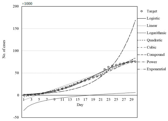
Figure 7. Fitness graph for China fitted by GWO.

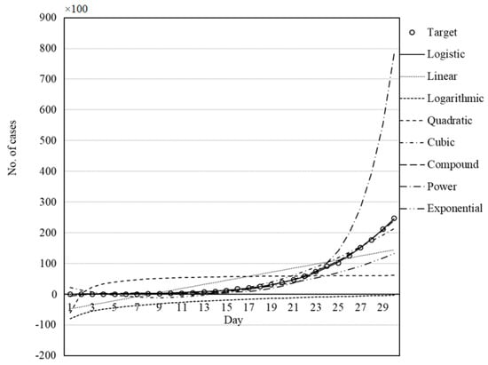
Figure 8. Set of models for Italy fitted by GWO.

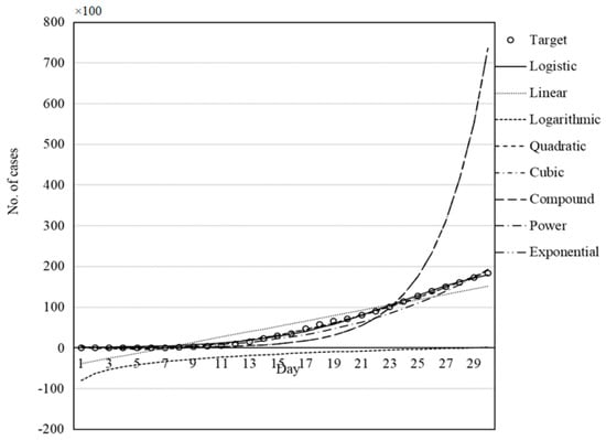
Figure 9. Set of models for Iran fitted by GWO.

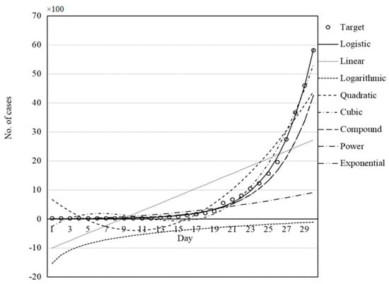
Figure 10. Set of models for Germany fitted by GWO.

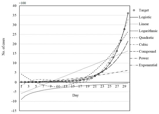
Figure 11. Set of models for USA fitted by GWO.

Figure 7, Figure 8, Figure 9, Figure 10 and Figure 11 illustrate the fit of the models investigated in this paper. The best fit for the prediction of COVID-19 cases was achieved for the logistic model followed by cubic and quadratic models for China (Figure 7), logistic followed by cubic models for Italy (Figure 8), cubic followed by logistic and quadratic models for Iran (Figure 9), the logistic model for Germany (Figure 10), and logistic model for the USA (Figure 11).

Machine Learning Results

This section presents the results for the training stage of ML methods. MLP and ANFIS were employed as single and hybrid ML methods, respectively. ML methods were trained using two datasets related to scenario 1 and scenario 2. Table 16 presents the results of the training phase.

Table 16. Results for the training phase of the ML methods.

	Scenario 1						Scenario 2
	MLP			ANFIS			MLP			ANFIS
	No. of Neurons	r	RMSE	MF Type	r	RMSE	No. of Neurons	r	RMSE	MF Type	r	RMSE
Italy	8	0.999	190.81	Tri.	0.999	189.76	8	0.999	199.52	Tri.	0.999	188.55
	12	0.999	194.84	Trap.	0.841	3743.63	12	0.999	195.79	Trap.	0.876	3276
	16	0.999	188.18	Gauss	0.998	320.93	16	0.999	195.2	Gauss	0.999	206.66
Average		0.999	191.27		0.946	1418.1	Average	0.999	196.83		0.958	1223.73
China	8	0.995	2287.55	Tri.	0.996	2293.09	8	0.996	2265.95	Tri.	0.996	2272.13
	12	0.996	2259.95	Trap.	0.987	4231.05	12	0.996	2285.73	Trap.	0.989	3835.34
	16	0.995	2407.16	Gauss	0.996	2358.3	16	0.996	2260.05	Gauss	0.996	2272.58
Average		0.995	2318.22		0.993	2960.81	Average	0.996	2270.57		0.993	2793.35
Iran	8	0.998	392.17	Tri.	0.998	395.33	8	0.998	404.21	Tri.	0.998	394.04
	12	0.998	391.04	Trap.	0.977	1282.33	12	0.998	392.77	Trap.	0.986	994
	16	0.998	392.19	Gauss	0.998	396.51	16	0.998	395.43	Gauss	0.998	391.96
Average		0.998	391.8		0.991	391.39	Average	0.998	397.47		0.994	593.33
Germany	8	0.999	55.6	Tri.	0.999	56.25	8	0.999	55.58	Tri.	0.999	55.63
	12	0.999	55.38	Trap.	0.12	1658.7	12	0.999	55.56	Trap.	0.13	1537.26
	16	0.999	55.58	Gauss	0.998	154.99	16	0.999	55.56	Gauss	0.999	62.91
Average		0.999	55.52		0.705	623.31	Average	0.999	55.56		0.709	551.93
USA	8	0.999	21.65	Tri.	0.999	21.75	8	0.999	22.31	Tri.	0.999	22.52
	12	0.999	22.36	Trap.	0.22	861.08	12	0.999	22.3	Trap.	0.2	935.41
	16	0.999	22.31	Gauss	0.998	86.32	16	0.999	22.4	Gauss	0.999	25.03
Average		0.999	22.1		0.739	323.05	Average	0.999	22.33		0.739	327.65

According to Table 16, the datasets related to scenarios 1 and 2 have different performance values. Accordingly, for Italy, the MLP with 16 neurons provided the highest accuracy for scenario 1 and ANFIS with Tri. MF provided the highest accuracy for scenario 2. By considering the average values of the RMSE and correlation coefficient, it can be concluded that scenario 1 is more suitable for modeling outbreak cases in Italy because it provides higher accuracy (the smallest RMSE and the largest correlation coefficient) than scenario 2.

For the dataset related to China, for both scenarios, MLP with 12 and 16 neurons, respectively for scenarios 1 and 2, provided the highest accuracy compared with the ANFIS model. By considering the average values of RMSE and correlation coefficient, it can be concluded that scenario 2 with a larger average correlation coefficient and smaller average RMSE than scenario 1 is more suitable for modeling the outbreak in China.

For the dataset of Iran, MLP with 12 neurons in the hidden layer for scenario 1 and ANFIS with Gaussian MF type for scenario 2 provided the best performance for the prediction of the outbreak. By considering the average values of the RMSE and correlation coefficient, it can be concluded that scenario 1 provided better performance than scenario 2. In addition, in general, the MLP has higher prediction accuracy compared with the ANFIS method.

In Germany, MLP with 12 neurons in its hidden layer provided the highest accuracy (smallest RMSE and largest correlation coefficient). By considering the average values of the RMSE and correlation coefficient, it can be concluded that scenario 1 is more suitable for the prediction of the outbreak in Germany than scenario 2.

In the USA, the MLP with 8 and 12 neurons, respectively, for scenarios 1 and 2, provided higher accuracy (the smallest RMSE and the largest correlation coefficient values) than the ANFIS model. By considering the average values of the RMSE and correlation coefficient values, it can be concluded that scenario 1 is more suitable than scenario 2, and MLP is more suitable than ANFIS for outbreak prediction.

Figure 12, Figure 13, Figure 14, Figure 15 and Figure 16 present the model fits for Italy, China, Iran, Germany, and the USA, respectively. By comparing Figure 12, Figure 13, Figure 14, Figure 15 and Figure 16 with Figure 7, Figure 8, Figure 9, Figure 10 and Figure 11, it can be concluded that the MLP and the logistic model fitted by GWO provided a better fit than the other models. In addition, the ML methods provided better performance compared with other models.

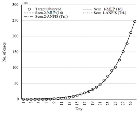
Figure 12. Set of models for Italy fitted by ML methods.

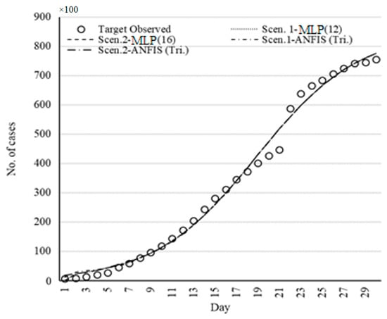
Figure 13. Set of models for China fitted by ML methods.

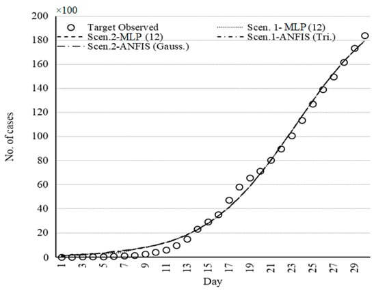
Figure 14. Set of models for Iran fitted by ML methods.

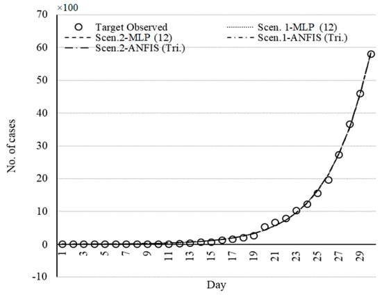
Figure 15. Set of models for Germany fitted by ML methods.

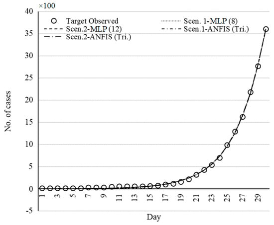
Figure 16. Set of models for USA fitted by ML methods.

Comparing the Fitted Models

This section presents a comparison of the accuracy and performance of the selected models for the prediction of 30 days’ outbreak. Figure 17, Figure 18, Figure 19, Figure 20 and Figure 21 show the deviation from the target values for the selected models.

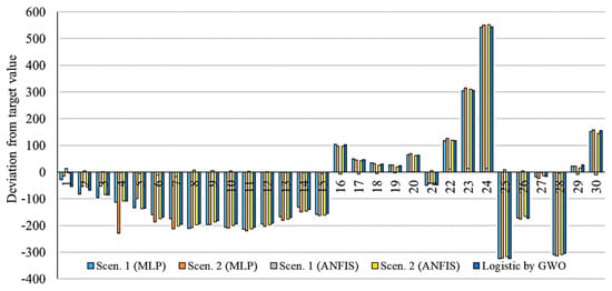
Figure 17. Deviation from target value for models related to Italy.

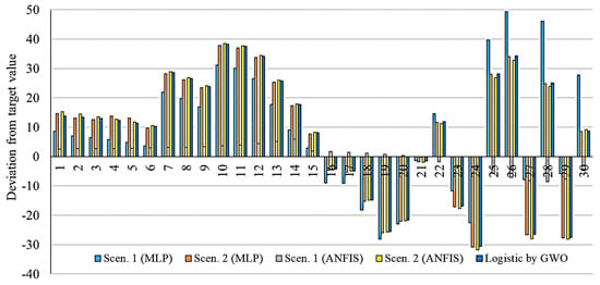
Figure 18. Deviation from target value for models related to China.

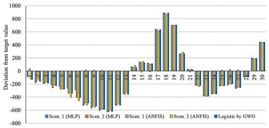
Figure 19. Deviation from target value for models related to Iran.

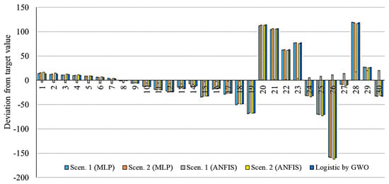
Figure 20. Deviation from target value for models related to Germany.

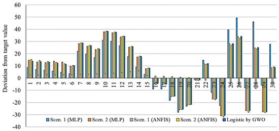
Figure 21. Deviation from target value for models related to USA.

As is clear from Figure 17, Figure 18, Figure 19, Figure 20 and Figure 21, the smallest deviation from the target values is related to the MLP for scenario 1 followed by MLP for scenario 2. This indicates the highest performance of the MLP method for the prediction of the outbreak. Figure 22, Figure 23, Figure 24, Figure 25 and Figure 26 present the outbreak prediction for 75 days and Table 17, Table 18, Table 19, Table 20 and Table 21 present the outbreak prediction for 150 days. Figure 27 represents the dispersion of the outbreak for the countries studied in this paper.

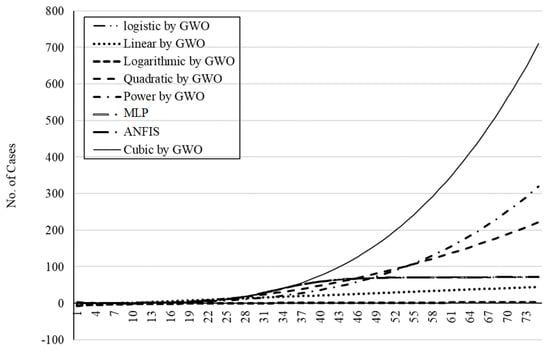
Figure 22. The outbreak prediction for Italy through 75 days.

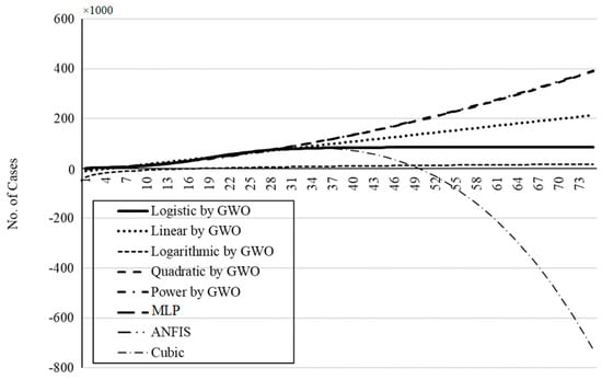
Figure 23. The outbreak prediction for China through 75 days.

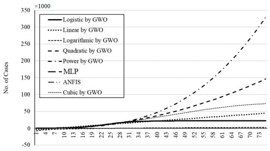
Figure 24. The outbreak prediction for Iran through 75 days.

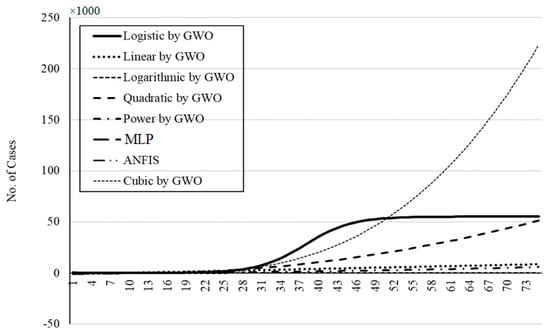
Figure 25. The outbreak prediction for Germany through 75 days.

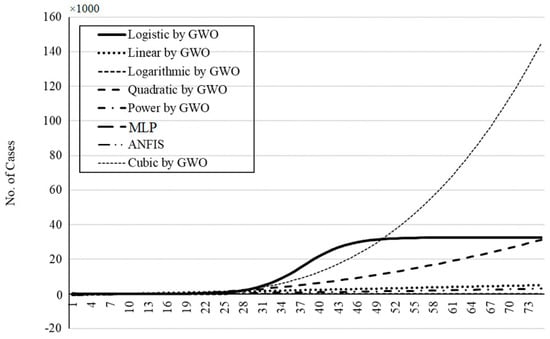
Figure 26. The outbreak prediction for the USA through 75 days.

Table 17. The outbreak prediction for Italy through 150 days.

	Logistic by GWO	Linear by GWO	Logarithmic by GWO	Quadratic by GWO	Power by GWO	MLP	ANFIS
Day 20th	3794.045	7837.054	−1280.93	5047.906	3225.523	3792.734	3796.738
Day 40th	58,966.55	21,111.37	273.235	47,914.4	35,898.08	58,966.74	58,964.96
Day 60th	70,571.86	34,385.68	1182.365	13,1597.7	14,6966.2	70,571.66	70,572.12
Day 80th	70,729.28	47,659.99	1827.402	256,097.8	399,523.4	70,729.27	70,729.15
Day 100th	70,731.06	60,934.31	2327.733	421,414.7	867,822	70,731.09	70,730.93
Day 120th	70,731.08	74,208.62	2736.532	627,548.4	1,635,643	70,731.14	70,730.87
Day 140th	70,731.08	87,482.94	3082.167	874,498.9	2,795,218	70,731.19	70,730.79
Day 150th	70,731.08	94,120.09	3236.862	1,013,280	3,552,851	70,731.21	70,730.75

Table 18. The outbreak prediction for China through 150 days.

	Logistic by GWO	Linear by GWO	Logarithmic by GWO	Quadratic by GWO	Power by GWO	MLP	ANFIS
Day 20th	47,397.6	47,218.47	1341.899	44,431.48	41,916.55	47,397.6	47,360.98
Day 40th	84,030.16	107,946.8	9507.249	134,729.1	135,599.1	84,030.17	84,030.39
Day 60th	84,996.7	168,675.1	14,283.67	265,812	269,471.3	84,996.7	84,996.67
Day 80th	85,011.08	229,403.4	17,672.6	437,680.2	438,660.2	85,011.08	85,011.05
Day 100th	85,011.29	290,131.7	20,301.26	650,333.6	640,132.8	85,011.3	85,011.22
Day 120th	85,011.3	350,860	22,449.02	903,772.3	871,733.6	85,011.34	85,011.13
Day 140th	85,011.3	411,588.3	24,264.94	1,197,996	1,131,815	85,011.38	85,011.05
Day 150th	85,011.3	441,952.5	25,077.68	1,360,403	1,272,113	85,011.41	85,011.01

Table 19. The outbreak prediction for Iran through 150 days.

	Logistic by GWO	Linear by GWO	Logarithmic by GWO	Quadratic by GWO	Power by GWO	MLP	ANFIS
Day 20th	6898.344	8593.676	−830.677	6993.955	5494.377	6902.315	6875.585
Day 40th	21,455.58	21,715.05	809.8719	37,087.98	47,060.48	21,457.4	21,456.65
Day 60th	21,931.01	34,836.43	1769.531	90,592.56	165,300.1	21,932.24	21,930.68
Day 80th	21,936	47,957.8	2450.42	167,507.7	403,082.8	21,935.1	21,935.54
Day 100th	21,936.05	61,079.18	2978.559	267,833.4	804,764.4	21,935.11	21,935.6
Day 120th	21,936.05	74,200.55	3410.08	391,569.6	1,415,829	21,935.12	21,935.63
Day 140th	21,936.05	87,321.93	3774.925	538,716.4	2,282,679	21,935.13	21,935.65
Day 150th	21,936.05	93,882.61	3938.219	621,068.7	2,826,737	21,935.13	21,935.67

Table 20. The outbreak prediction for Germany through 150 days.

	Logistic by GWO	Linear by GWO	Logarithmic by GWO	Quadratic by GWO	Power by GWO	MLP	ANFIS
Day 20th	431.027	1438.128	−279.772	763.1467	400.0548	432.8991	431.8119
Day 40th	35,356.27	4006.551	9.199328	10,492.96	1624.405	35,355.14	35,355.72
Day 60th	55,043.44	6574.974	178.2366	30,100.56	3687.126	55,036.14	55,044.03
Day 80th	55,179.07	9143.397	298.1705	59,585.93	6595.829	55,179.05	55,178.88
Day 100th	55,179.67	11,711.82	391.1984	98,949.09	10,355.87	55,179.9	55,179.47
Day 120th	55,179.67	14,280.24	467.2078	148,190	14,971.42	55,179.92	55,179.42
Day 140th	55,179.67	16,848.66	531.4728	207,308.7	20,445.86	55,179.94	55,179.37
Day 150th	55,179.67	18,132.88	560.2357	240,572.3	23,506.09	55,179.96	55,179.35

Table 21. The outbreak prediction for the USA for 150 days.

	Logistic by GWO	Linear by GWO	Logarithmic by GWO	Quadratic by GWO	Power by GWO	MLP	ANFIS
Day 20th	242.6091	869.8855	−156.73	456.0663	309.616	244.0038	243.6504
Day 40th	21,951.15	2406.562	15.85698	6383.264	1031.324	21,942.25	21,948.25
Day 60th	32,547.08	3943.238	116.8138	18,366.35	2084.876	32,552.6	32,548.47
Day 80th	32,604.34	5479.914	188.4437	36,405.33	3435.319	32,606.19	32,604.47
Day 100th	32,604.55	7016.591	244.0043	60,500.21	5060.548	32,606.63	32,604.72
Day 120th	32,604.55	8553.267	289.4005	90,650.97	6944.676	32,606.7	32,604.76
Day 140th	32,604.55	10,089.94	327.7825	126,857.6	9075.446	32,606.78	32,604.8
Day 150th	32,604.55	10,858.28	344.9611	147,231.9	10,230.16	32,606.81	32,604.82

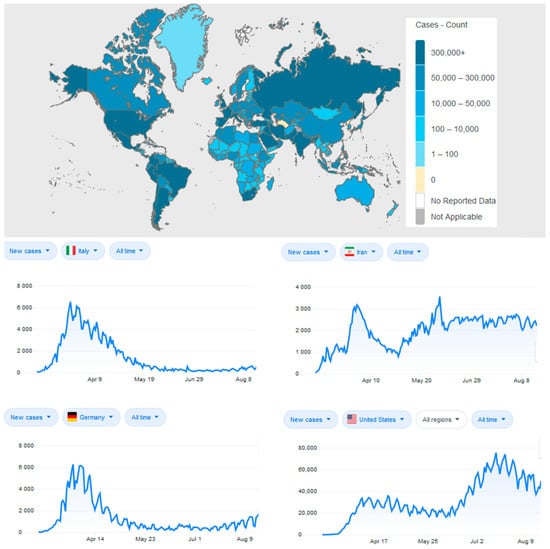
Figure 27. An overview of the current state of the COVID-19 outbreak including daily cases for the four countries of the study (source: World Health Organization).

4. Discussion

The parameters of several simple mathematical models (i.e., logistic, linear, logarithmic, quadratic, cubic, compound, power, and exponential) were fitted using GA, PSO, and GWO. The logistic model outperformed other methods and showed promising results based on training for 30 days. Extrapolation of the prediction beyond the original observation range of 30 days should not be expected to be realistic considering the new statistics. The fitted models generally showed low accuracy and also weak generalization ability for the five countries. Although the prediction for China was promising, the model was insufficient for extrapolation, as expected. In turn, the logistic GWO outperformed the PSO and GA, and the computational cost for GWO was reported as satisfactory. Consequently, for further assessment of the ML models, the logistic model fitted with GWO was used for comparative analysis.

In the next step, for introducing the machine learning methods for time-series prediction, two scenarios were proposed. Scenario 1 considered four data samples from the progress of the infection from previous days, as reported in Table 2. The sampling for data processing was done weekly for scenario 1. However, scenario 2 was devoted to daily sampling for all previous consecutive days. Providing these two scenarios expanded the scope of this study. Training and test results for the two machine learning models (MLP and ANFIS) were considered for the two scenarios. A detailed investigation was also carried out to explore the most suitable number of neurons. For the MLP, the performances of using 8, 12, and 16 neurons were analyzed throughout the study. For the ANFIS, the membership function (MF) types of Tri, Trap, and Gauss were analyzed throughout the study. The five counties of Italy, China, Iran, Germany, and USA were considered. The performance of both ML models for these countries varied between the two different scenarios. Given the observed results, it is not possible to select the most suitable scenario. Therefore, both daily and weekly sampling can be used in machine learning modeling. Comparison between analytical and machine learning models using the deviation from the target value (Figure 17, Figure 18, Figure 19, Figure 20 and Figure 21) indicated that the MLP in both scenarios delivered the most accurate results. Extrapolation for long-term prediction of up to 150 days using the ML models was tested. The actual prediction of MLP and ANFIS for the five countries was reported and showed the progression of the outbreak.

This paper evaluated the applicability of two machine learning models, MLP and ANFIS, for predicting the COVID-19 outbreak. The models showed promising results in terms of predicting the time series without the assumptions that epidemiological models require. Machine learning models, as an alternative to epidemiological models, showed potential in predicting COVID-19, as they did for modeling other outbreaks (see Table 1). Considering the availability of only a small amount of training data, it is expected that machine learning will be developed further as the basis for, or a component of, future outbreak prediction models.

Here, it is worth mentioning that machine learning can also be found useful in dealing with the challenges that SEIR models face for COVID-19. For example, the number of cases reported by worldometer is not the number of infected (E in the SEIR model). For example, the number of cases reported by worldometer for the UK situation is the number of people tested. In addition, data for the number of infectious people (I in SEIR) is a challenging matter because many people who might be infectious may not choose to be for tested if, for example, their symptoms are mild. Although better data exist on the number of people who are admitted to hospital and the number who die, these also do not represent R because it is generally accepted that most people with COVID-19 recover without entering hospital. Considering this data problem, it is extremely difficult to fit SEIR models satisfactorily. Considering such challenges, for future research, the ability of machine learning for estimation of the missing information on the number of exposed E or infected can be evaluated. Furthermore, the temporal non-stationarity data in control measures can also be investigated using machine learning.

5. Conclusions

The global pandemic of the severe acute respiratory syndrome coronavirus 2 (SARS-CoV-2) has become the primary national security issue of many nations. Advancement of accurate prediction models for the outbreak is essential to provide insights into the spread and consequences of this infectious disease. Due to the high level of uncertainty and lack of crucial data, standard epidemiological models have shown low accuracy for long-term prediction. This paper presents a comparative analysis of ML and soft computing models to predict the COVID-19 outbreak. The results of two ML models (MLP and ANFIS) reported a high generalization ability for long-term prediction. With respect to the results reported in this paper and due to the highly complex nature of the COVID-19 outbreak and differences among nations, this study suggests ML as an effective tool to model the time series of the outbreak. We should note that this paper provides an initial benchmarking to demonstrate the potential of machine learning for future research.

For the advancement of higher performance models for long-term prediction, future research should be devoted to comparative studies on various ML models for individual countries. Due to the fundamental differences between the outbreak in various countries, advancement of global models with generalization ability would not be feasible. As observed and reported in many studies, it is unlikely that an individual outbreak will be replicated elsewhere [1].

Although the most difficult prediction is to estimate the maximum number of infected patients, estimation of the individual mortality rate (n(deaths)/n(infected)) is also essential. The mortality rate is particularly important to accurately estimate the number of patients and the required beds in intensive care units. For future research, modeling the mortality rate would be of the utmost importance for nations to plan for new facilities. For future research, integration of machine learning and SIR/SEIR models is suggested to enhance the existing standard epidemiological models in terms of accuracy and longer lead time.

References

- Remuzzi, A.; Remuzzi, G. COVID-19 and Italy: What next? Lancet 2020, 395, 1225–1228. [Google Scholar] [CrossRef]
- Ivanov, D. Predicting the impacts of epidemic outbreaks on global supply chains: A simulation-based analysis on the coronavirus outbreak (COVID-19/SARS-CoV-2) case. Transp. Res. Part E 2020, 136, 101922. [Google Scholar] [CrossRef]
- Koolhof, I.S.; Gibney, K.B.; Bettiol, S.; Charleston, M.; Wiethoelter, A.; Arnold, A.-L.; Campbell, P.T.; Neville, P.J.; Aung, P.; Shiga, T.; et al. The forecasting of dynamical Ross River virus outbreaks: Victoria, Australia. Epidemics 2020, 30, 100377. [Google Scholar] [CrossRef] [PubMed]
- Darwish, A.; Rahhal, Y.; Jafar, A. A comparative study on predicting influenza outbreaks using different feature spaces: Application of influenza-like illness data from Early Warning Alert and Response System in Syria. BMC Res. Notes 2020, 13, 33. [Google Scholar] [CrossRef] [PubMed]
- Rypdal, M.; Sugihara, G. Inter-outbreak stability reflects the size of the susceptible pool and forecasts magnitudes of seasonal epidemics. Nat. Commun. 2019, 10, 2374. [Google Scholar] [CrossRef] [PubMed]
- Scarpino, S.V.; Petri, G. On the predictability of infectious disease outbreaks. Nat. Commun. 2019, 10, 898. [Google Scholar] [CrossRef]
- Zhan, Z.; Dong, W.; Lu, Y.; Yang, P.; Wang, Q.; Jia, P. Real-Time Forecasting of Hand-Foot-and-Mouth Disease Outbreaks using the Integrating Compartment Model and Assimilation Filtering. Sci. Rep. 2019, 9, 2661. [Google Scholar] [CrossRef] [PubMed]
- Koike, F.; Morimoto, N. Supervised forecasting of the range expansion of novel non-indigenous organisms: Alien pest organisms and the 2009 H1N1 flu pandemic. Glob. Ecol. Biogeogr. 2018, 27, 991–1000. [Google Scholar] [CrossRef]
- Dallas, T.; Carlson, C.J.; Poisot, T. Testing predictability of disease outbreaks with a simple model of pathogen biogeography. R. Soc. Open Sci. 2019, 6, 190883. [Google Scholar] [CrossRef] [PubMed]
- De Groot, M.; Ogris, N. Short-term forecasting of bark beetle outbreaks on two economically important conifer tree species. For. Ecol. Manag. 2019, 450, 117495. [Google Scholar] [CrossRef]
- Kelly, J.D.; Park, J.; Harrigan, R.J.; Hoff, N.A.; Lee, S.D.; Wannier, S.R.; Selo, B.; Mossoko, M.; Njoloko, B.; Okitolonda-Wemakoy, E.; et al. Real-time predictions of the 2018–2019 Ebola virus disease outbreak in the Democratic Republic of the Congo using Hawkes point process models. Epidemics 2019, 28, 100354. [Google Scholar] [CrossRef] [PubMed]
- Maier, B.F.; Brockmann, D. Effective containment explains sub-exponential growth in confirmed cases of recent COVID-19 outbreak in Mainland China. medRxiv 2020. [Google Scholar] [CrossRef]
- Pan, J.-R.; Huang, Z.-Q.; Chen, K. Evaluation of the effect of varicella outbreak control measures through a discrete time delay SEIR model. Zhonghua Yu Fang Yi Xue Za Zhi 2012, 46, 343–347. [Google Scholar] [PubMed]
- Zha, W.-T.; Pang, F.-R.; Zhou, N.; Wu, B.; Liu, Y.; Du, Y.-B.; Hong, X.-Q.; Lv, Y. Research about the optimal strategies for prevention and control of varicella outbreak in a school in a central city of China: Based on an SEIR dynamic model. Epidemiol. Infect. 2020, 148, e56. [Google Scholar] [CrossRef] [PubMed]
- Dantas, E.; Tosin, M.; Cunha, A., Jr. Calibration of a SEIR–SEI epidemic model to describe the Zika virus outbreak in Brazil. Appl. Math. Comput. 2018, 338, 249–259. [Google Scholar] [CrossRef]
- Leonenko, V.N.; Ivanov, S.V. Fitting the SEIR model of seasonal influenza outbreak to the incidence data for Russian cities. Russ. J. Numer. Anal. Math. Model. 2016, 31, 267–279. [Google Scholar] [CrossRef]
- Imran, M.; Usman, M.; Dur-E-Ahmad, M.; Khan, A. Transmission Dynamics of Zika Fever: A SEIR Based Model. Differ. Equ. Dyn. Syst. 2017, 1–24. [Google Scholar] [CrossRef]
- Miranda, G.H.B.; Baetens, J.M.; Bossuyt, N.; Bruno, O.M.; De Baets, B. Real-time prediction of influenza outbreaks in Belgium. Epidemics 2019, 28, 100341. [Google Scholar] [CrossRef]
- Sinclair, D.R.; Grefenstette, J.J.; Krauland, M.G.; Galloway, D.D.; Frankeny, R.J.; Travis, C.; Burke, N.S.; Roberts, M.S. Forecasted Size of Measles Outbreaks Associated With Vaccination Exemptions for Schoolchildren. JAMA Netw. Open 2019, 2, e199768. [Google Scholar] [CrossRef]
- Zhao, S.; Musa, S.S.; Fu, H.; He, D.; Qin, J. Simple framework for real-time forecast in a data-limited situation: The Zika virus (ZIKV) outbreaks in Brazil from 2015 to 2016 as an example. Parasites Vectors 2019, 12, 344. [Google Scholar] [CrossRef]
- Fast, S.M.; Kim, L.; Cohn, E.L.; Mekaru, S.R.; Brownstein, J.S.; Markuzon, N. Predicting social response to infectious disease outbreaks from internet-based news streams. Ann. Oper. Res. 2018, 263, 551–564. [Google Scholar] [CrossRef] [PubMed]
- McCabe, C.M.; Nunn, C. Effective Network Size Predicted From Simulations of Pathogen Outbreaks Through Social Networks Provides a Novel Measure of Structure-Standardized Group Size. Front. Vet. Sci. 2018, 5, 71. [Google Scholar] [CrossRef] [PubMed]
- Bragazzi, N.L.; Mahroum, N.; Cruvinel, T.; Mavragani, A. Google Trends Predicts Present and Future Plague Cases During the Plague Outbreak in Madagascar: Infodemiological Study. JMIR Public Health Surveill. 2019, 5, e13142. [Google Scholar] [CrossRef] [PubMed]
- Jain, R.; Sontisirikit, S.; Iamsirithaworn, S.; Prendinger, H. Prediction of dengue outbreaks based on disease surveillance, meteorological and socio-economic data. BMC Infect. Dis. 2019, 19, 272. [Google Scholar] [CrossRef]
- Kim, T.H.; Hong, K.J.; Shin, S.D.; Park, G.J.; Kim, S.; Hong, N. Forecasting respiratory infectious outbreaks using ED-based syndromic surveillance for febrile ED visits in a Metropolitan City. Am. J. Emerg. Med. 2019, 37, 183–188. [Google Scholar] [CrossRef]
- Zhong, L.; Mu, L.; Li, J.; Wang, J.; Yin, Z.; Liu, D. Early Prediction of the 2019 Novel Coronavirus Outbreak in the Mainland China Based on Simple Mathematical Model. IEEE Access 2020, 8, 51761–51769. [Google Scholar] [CrossRef]
- Wu, J.T.; Leung, K.; Leung, G.M. Nowcasting and forecasting the potential domestic and international spread of the 2019-nCoV outbreak originating in Wuhan, China: A modelling study. Lancet 2020, 395, 689–697. [Google Scholar] [CrossRef]
- Reis, J.; Yamana, T.K.; Kandula, S.; Shaman, J. Superensemble forecast of respiratory syncytial virus outbreaks at national, regional, and state levels in the United States. Epidemics 2019, 26, 1–8. [Google Scholar] [CrossRef]
- Burke, R.M.; Shah, M.P.; Wikswo, M.E.; Barclay, L.; Kambhampati, A.; Marsh, Z.; Cannon, J.L.; Parashar, U.D.; Vinjé, J.; Hall, A.J. The Norovirus Epidemiologic Triad: Predictors of Severe Outcomes in US Norovirus Outbreaks, 2009–2016. J. Infect. Dis. 2019, 219, 1364–1372. [Google Scholar] [CrossRef]
- Carlson, C.J.; Dougherty, E.R.; Boots, M.; Getz, W.M.; Ryan, S.J. Consensus and conflict among ecological forecasts of Zika virus outbreaks in the United States. Sci. Rep. 2018, 8, 4921. [Google Scholar] [CrossRef]
- Kleiven, E.F.; Henden, J.; Ims, R.A.; Yoccoz, N.G. Seasonal difference in temporal transferability of an ecological model: Near-term predictions of lemming outbreak abundances. Sci. Rep. 2018, 8, 15252. [Google Scholar] [CrossRef] [PubMed]
- Rivers-Moore, N.A.; Hill, T. A predictive management tool for blackfly outbreaks on the Orange River, South Africa. River Res. Appl. 2018, 34, 1197–1207. [Google Scholar] [CrossRef]
- Yin, R.; Tran, V.H.; Zhou, X.; Zheng, J.; Kwoh, C.K. Predicting antigenic variants of H1N1 influenza virus based on epidemics and pandemics using a stacking model. PLoS ONE 2018, 13, e0207777. [Google Scholar] [CrossRef] [PubMed]
- Agarwal, N.; Koti, S.R.; Saran, S.; Kumar, A.S. Data Mining Techniques for Predicting Dengue Outbreak in Geospatial Domain Using Weather Parameters for New Delhi, India. Curr. Sci. 2018, 114, 2281–2291. [Google Scholar] [CrossRef]
- Anno, S.; Hara, T.; Kai, H.; Lee, M.-A.; Chang, Y.; Oyoshi, K.; Mizukami, Y.; Tadono, T. Spatiotemporal dengue fever hotspots associated with climatic factors in Taiwan including outbreak predictions based on machine-learning. Geospat. Health 2019, 14, 183–194. [Google Scholar] [CrossRef] [PubMed]
- Chenar, S.S.; Deng, Z. Development of artificial intelligence approach to forecasting oyster norovirus outbreaks along Gulf of Mexico coast. Environ. Int. 2018, 111, 212–223. [Google Scholar] [CrossRef] [PubMed]
- Chenar, S.S.; Deng, Z. Development of genetic programming-based model for predicting oyster norovirus outbreak risks. Water Res. 2018, 128, 20–37. [Google Scholar] [CrossRef] [PubMed]
- Iqbal, N.; Islam, M. Machine learning for dengue outbreak prediction: A performance evaluation of different prominent classifiers. Informatica 2019, 43, 363–371. [Google Scholar] [CrossRef]
- Liang, R.; Lu, Y.; Qu, X.; Su, Q.; Li, C.; Xia, S.; Liu, Y.; Zhang, Q.; Cao, X.; Chen, Q.; et al. Prediction for global African swine fever outbreaks based on a combination of random forest algorithms and meteorological data. Transbound. Emerg. Dis. 2020, 67, 935–946. [Google Scholar] [CrossRef]
- Mezzatesta, S.; Torino, C.; De Meo, P.; Fiumara, G.; Vilasi, A. A machine learning-based approach for predicting the outbreak of cardiovascular diseases in patients on dialysis. Comput. Methods Programs Biomed. 2019, 177, 9–15. [Google Scholar] [CrossRef]
- Raja, D.B.; Mallol, R.; Ting, C.Y.; Kamaludin, F.; Ahmad, R.; Ismail, S.; Jayaraj, V.J.; Sundram, B.M. Artificial Intelligence Model as Predictor for Dengue Outbreaks. Malays. J. Public Health Med. 2019, 19, 103–108. [Google Scholar] [CrossRef]
- Tapak, L.; Hamidi, O.; Fathian, M.; Karami, M. Comparative evaluation of time series models for predicting influenza outbreaks: Application of influenza-like illness data from sentinel sites of healthcare centers in Iran. BMC Res. Notes 2019, 12, 1–6. [Google Scholar] [CrossRef] [PubMed]
- Muurlink, O.; Stephenson, P.; Islam, M.Z.; Taylor-Robinson, A.W. Long-term predictors of dengue outbreaks in Bangladesh: A data mining approach. Infect. Dis. Model. 2018, 3, 322–330. [Google Scholar] [CrossRef] [PubMed]
- Choubin, B.; Mosavi, A.; Alamdarloo, E.H.; Hosseini, F.S.; Shamshirband, S.; Dashtekian, K.; Ghamisi, P. Earth fissure hazard prediction using machine learning models. Environ. Res. 2019, 179, 108770. [Google Scholar] [CrossRef]
- Choubin, B.; Abdolshahnejad, M.; Moradi, E.; Querol, X.; Mosavi, A.; Shamshirband, S.; Ghamisi, P. Spatial hazard assessment of the PM10 using machine learning models in Barcelona, Spain. Sci. Total Environ. 2020, 701, 134474. [Google Scholar] [CrossRef]
- Reported Cases and Deaths by Country, Territory, or Conveyance. Available online: https://www.worldometers.info/coronavirus/#countries (accessed on 30 September 2020).
- Back, T. Evolutionary Algorithms in Theory and Practice: Evolution Strategies, Evolutionary Programming, Genetic Algorithms; Oxford University Press: Oxford, UK, 1996. [Google Scholar]
- Deb, K. Multi-Objective Optimization Using Evolutionary Algorithms; John Wiley & Sons: Hoboken, NJ, USA, 2001; Volume 16. [Google Scholar]
- Zitzler, E.; Deb, K.; Thiele, L. Comparison of Multiobjective Evolutionary Algorithms: Empirical Results. Evol. Comput. 2000, 8, 173–195. [Google Scholar] [CrossRef]
- Ghamisi, P.; Benediktsson, J.A. Feature Selection Based on Hybridization of Genetic Algorithm and Particle Swarm Optimization. IEEE Geosci. Remote. Sens. Lett. 2014, 12, 309–313. [Google Scholar] [CrossRef]
- Dineva, A.A.; Mosavi, A.; Ardabili, S.F.; Vajda, I.; Shamshirband, S.; Rabczuk, T.; Chau, K.-W. Review of Soft Computing Models in Design and Control of Rotating Electrical Machines. Energies 2019, 12, 1049. [Google Scholar] [CrossRef]
- Mosavi, A.; Salimi, M.; Ardabili, S.F.; Rabczuk, T.; Shamshirband, S.; Várkonyi-Kóczy, A.R. State of the Art of Machine Learning Models in Energy Systems, a Systematic Review. Energies 2019, 12, 1301. [Google Scholar] [CrossRef]
- Mühlenbein, H.; Schomisch, M.; Born, J. The parallel genetic algorithm as function optimizer. Parallel Comput. 1991, 17, 619–632. [Google Scholar] [CrossRef]
- Whitley, D. A genetic algorithm tutorial. Stat. Comput. 1994, 4, 65–85. [Google Scholar] [CrossRef]
- Horn, J.; Nafpliotis, N.; Goldberg, D.E. A niched Pareto genetic algorithm for multiobjective optimization. In Proceedings of the First IEEE Conference on Evolutionary Computation: IEEE World Congress on Computational Intelligence, Orlando, FL, USA, 27–29 June 2002; pp. 82–87. [Google Scholar]
- Reeves, C.R. A genetic algorithm for flowshop sequencing. Comput. Oper. Res. 1995, 22, 5–13. [Google Scholar] [CrossRef]
- Jones, G.; Willett, P.; Glen, R.C.; Leach, A.R.; Taylor, R. Development and validation of a genetic algorithm for flexible docking. J. Mol. Biol. 1997, 267, 727–748. [Google Scholar] [CrossRef] [PubMed]
- Ardabili, S.F.; Mosavi, A.; Várkonyi-Kóczy, A.R. Advances in Machine Learning Modeling Reviewing Hybrid and Ensemble Methods. In Proceedings of the 18th International Conference on Global Research and Education, Budapest, Hungary, 4–9 September 2020; pp. 215–227. [Google Scholar]
- Houck, C.R.; Joines, J.; Kay, M.G. A genetic algorithm for function optimization: A Matlab implementation. Ncsu-ie tr 1995, 95, 1–10. [Google Scholar]
- Whitley, D.; Starkweather, T.; Bogart, C. Genetic algorithms and neural networks: Optimizing connections and connectivity. Parallel Comput. 1990, 14, 347–361. [Google Scholar] [CrossRef]
- Kennedy, J.; Eberhart, R. Particle swarm optimization. In Proceedings of the ICNN’95-International Conference on Neural Networks, Perth, WA, Australia, 27 November–1 December 1995; pp. 1942–1948. [Google Scholar]
- Poli, R.; Kennedy, J.; Blackwell, T. Particle swarm optimization. Swarm Intell. 2007, 1, 33–57. [Google Scholar] [CrossRef]
- Clerc, M. Particle Swarm Optimization; John Wiley & Sons: Hoboken, NJ, USA, 2010; Volume 93. [Google Scholar]
- Angeline, P.J. Using selection to improve particle swarm optimization. In Proceedings of the 1998 IEEE International Conference on Evolutionary Computation Proceedings IEEE World Congress on Computational Intelligence (Cat No 98TH8360), Anchorage, AK, USA, 4–9 May 1988; pp. 84–89. [Google Scholar]
- Sun, J.; Feng, B.; Xu, W. Particle swarm optimization with particles having quantum behavior. In Proceedings of the 2004 Congress on Evolutionary Computation (IEEE Cat No 04TH8753), Portland, OR, USA, 19–23 June 2004; pp. 325–331. [Google Scholar]
- Parsopoulos, K.; Vrahatis, M. Recent approaches to global optimization problems through Particle Swarm Optimization. Nat. Comput. 2002, 1, 235–306. [Google Scholar] [CrossRef]
- Bai, Q. Analysis of Particle Swarm Optimization Algorithm. Comput. Inf. Sci. 2010, 3, 180. [Google Scholar] [CrossRef]
- Parsopoulos, K.E.; Vrahatis, M.N. Particle swarm optimization method in multiobjective problems. In Proceedings of the 2002 ACM Symposium on Applied Computing, Madrid, Spain, 10–14 March 2002; pp. 603–607. [Google Scholar]
- Ghamisi, P.; Couceiro, M.S.; Benediktsson, J.A.; Ferreira, N.M.F. An efficient method for segmentation of images based on fractional calculus and natural selection. Expert Syst. Appl. 2012, 39, 12407–12417. [Google Scholar] [CrossRef]
- Ghamisi, P.; Couceiro, M.S.; Martins, F.M.L.; Benediktsson, J.A. Multilevel Image Segmentation Based on Fractional-Order Darwinian Particle Swarm Optimization. IEEE Trans. Geosci. Remote. Sens. 2013, 52, 2382–2394. [Google Scholar] [CrossRef]
- Mirjalili, S.; Mirjalili, S.M.; Lewis, A. Grey Wolf Optimizer. Adv. Eng. Softw. 2014, 69, 46–61. [Google Scholar] [CrossRef]
- Ardabili, S.; Mosavi, A.; Varkonyi-Koczy, A. Building Energy information: Demand and consumption prediction with Machine Learning models for sustainable and smart cities. In Proceedings of the 18th International Conference on Global Research and Education, Budapest, Hungary, 4–7 September 2019. [Google Scholar]
- Ardabili, S.F.; Mosavi, A.; Várkonyi-Kóczy, A.R. Systematic Review of Deep Learning and Machine Learning Models in Biofuels Research. In Proceedings of the 18th International Conference on Global Research and Education, Budapest, Hungary, 4–7 September 2019. [Google Scholar]
- Gundoshmian, T.M.; Ardabili, S.F.; Mosavi, A.; Várkonyi-Kóczy, A.R. Prediction of Combine Harvester Performance Using Hybrid Machine Learning Modeling and Response Surface Methodology. In Proceedings of the 18th International Conference on Global Research and Education, Budapest, Hungary, 4–7 September 2019. [Google Scholar]
- Fotovatikhah, F.; Herrera, M.; Shamshirband, S.; Chau, K.-W.; Ardabili, S.F.; Piran, J. Survey of computational intelligence as basis to big flood management: Challenges, research directions and future work. Eng. Appl. Comput. Fluid Mech. 2018, 12, 411–437. [Google Scholar] [CrossRef]
- Hamilton, J.D. Time Series Analysis; Princeton University Press: Princeton, NJ, USA, 1994; Volume 2. [Google Scholar]
- Ardabili, S.F.; Mosavi, A.; Mahmoudi, A.; Gundoshmian, T.M.; Nosratabadi, S.; Várkonyi-Kóczy, A.R. Modelling Temperature Variation of Mushroom Growing Hall Using Artificial Neural Networks. In Proceedings of the 18th International Conference on Global Research and Education, Budapest, Hungary, 4–7 September 2019. [Google Scholar]
- Khosravi, A.; Koury, R.; Machado, L.; Pabon, J.J. Prediction of wind speed and wind direction using artificial neural network, support vector regression and adaptive neuro-fuzzy inference system. Sustain. Energy Technol. Assess. 2018, 25, 146–160. [Google Scholar] [CrossRef]
- Amid, S.; Gundoshmian, T.M. Prediction of output energies for broiler production using linear regression, ANN (MLP, RBF), and ANFIS models. Environ. Prog. Sustain. Energy 2017, 36, 577–585. [Google Scholar] [CrossRef]
- Hossain, M.A.; Ayodele, B.V.; Cheng, C.K.; Khan, M.R. Artificial neural network modeling of hydrogen-rich syngas production from methane dry reforming over novel Ni/CaFe2O4 catalysts. Int. J. Hydrog. Energy 2016, 41, 11119–11130. [Google Scholar] [CrossRef]
- Taghavifar, H.; Mardani, A. Wavelet neural network applied for prognostication of contact pressure between soil and driving wheel. Inf. Process. Agric. 2014, 1, 51–56. [Google Scholar] [CrossRef][Green Version]
- Sharabiani, V.; Kassar, F.; Gilandeh, Y.; Ardabili, S. Application of Soft Computing Methods and Spectral Reflectance Data for Wheat Growth Monitoring. Iraqi J. Agric. Sci. 2019, 50, 1064–1076. [Google Scholar]
- Mirzazadeh, A.; Abdollahpour, S.; Mahmoudi, A.; Bukat, A. Intelligent modeling of material separation in combine harvester’s thresher by ANN. Int. J. Agric. Crop Sci. 2012, 4, 1767–1777. [Google Scholar]
- Khalesi, S.; Mahmoudi, A.; Hosainpour, A.; Alipour, A. Detection of Walnut Varieties Using Impact Acoustics and Artificial Neural Networks (ANNs). Mod. Appl. Sci. 2012, 6, 43. [Google Scholar] [CrossRef][Green Version]
- Reshadsedghi, A.; Mahmoudi, A. Detection of almond varieties using impact acoustics and artificial neural networks. Int. J. Agric. Crop Sci. 2013, 6, 1008. [Google Scholar]
- Hassoun, M.H. Fundamentals of Artificial Neural Networks; MIT Press: Cambridge, MA, USA, 1995. [Google Scholar]
- Jang, J.-S.R. ANFIS: Adaptive-network-based fuzzy inference system. IEEE Trans. Syst. Man Cybern. 1993, 23, 665–685. [Google Scholar] [CrossRef]
- Ardabili, S.F.; Mahmoudi, A.; Gundoshmian, T.M. Modeling and simulation controlling system of HVAC using fuzzy and predictive (radial basis function, RBF) controllers. J. Build. Eng. 2016, 6, 301–308. [Google Scholar] [CrossRef]
- Amid, S.; Gundoshmian, T.M. Prediction of Output Energy based on Different Energy Inputs on Broiler Production using Application of Adaptive Neural-Fuzzy Inference System. Agric. Sci. Dev. 2016, 5, 14–21. [Google Scholar] [CrossRef]
- Ardabili, S.F.; Mosavi, A.; Dehghani, M.; Várkonyi-Kóczy, A.R. Deep Learning and Machine Learning in Hydrological Processes Climate Change and Earth Systems a Systematic Review. In Proceedings of the 18th International Conference on Global Research and Education, Budapest, Hungary, 4–7 September 2019; pp. 52–62. [Google Scholar]
- Nosratabadi, S.; Mosavi, A.; M-Keivani, R.; Ardabili, S.F.; Aram, F. State of the Art Survey of Deep Learning and Machine Learning Models for Smart Cities and Urban Sustainability. In Proceedings of the 18th International Conference on Global Research and Education, Budapest, Hungary, 4–7 September 2019; pp. 228–238. [Google Scholar]
- Güler, I.; Übeyli, E.D. Adaptive neuro-fuzzy inference system for classification of EEG signals using wavelet coefficients. J. Neurosci. Methods 2005, 148, 113–121. [Google Scholar] [CrossRef] [PubMed]
- Chang, J.-R.; Wei, L.-Y.; Cheng, C.-H. A hybrid ANFIS model based on AR and volatility for TAIEX forecasting. Appl. Soft Comput. 2011, 11, 1388–1395. [Google Scholar] [CrossRef]
- Chang, F.-J.; Chang, Y.-T. Adaptive neuro-fuzzy inference system for prediction of water level in reservoir. Adv. Water Resour. 2006, 29, 1–10. [Google Scholar] [CrossRef]
- Moghaddamnia, A.; Gousheh, M.G.; Piri, J.; Amin, S.; Han, D. Evaporation estimation using artificial neural networks and adaptive neuro-fuzzy inference system techniques. Adv. Water Resour. 2009, 32, 88–97. [Google Scholar] [CrossRef]
- Çaydaş, U.; Hasçalık, A.; Ekici, S. An adaptive neuro-fuzzy inference system (ANFIS) model for wire-EDM. Expert Syst. Appl. 2009, 36, 6135–6139. [Google Scholar] [CrossRef]
- Yadav, D.; Chhabra, D.; Gupta, R.K.; Phogat, A.; Ahlawat, A. Modeling and analysis of significant process parameters of FDM 3D printer using ANFIS. Mater. Today Proc. 2020, 21, 1592–1604. [Google Scholar] [CrossRef]
- Ardabili, S.F.; Mahmoudi, A.; Gundoshmian, T.M.; Roshanianfard, A. Modeling and comparison of fuzzy and on/off controller in a mushroom growing hall. Measurement 2016, 90, 127–134. [Google Scholar] [CrossRef]
Publisher’s Note: MDPI stays neutral with regard to jurisdictional claims in published maps and institutional affiliations. |
© 2020 by the authors. Licensee MDPI, Basel, Switzerland. This article is an open access article distributed under the terms and conditions of the Creative Commons Attribution (CC BY) license (http://creativecommons.org/licenses/by/4.0/).