Spatial–Spectral Squeeze-and-Excitation Residual Network for Hyperspectral Image Classification

Abstract

Jointly using spectral and spatial information has become a mainstream strategy in the field of hyperspectral image (HSI) processing, especially for classification. However, due to the existence of noisy or correlated spectral bands in the spectral domain and inhomogeneous pixels in the spatial neighborhood, HSI classification results are often degraded and unsatisfactory. Motivated by the attention mechanism, this paper proposes a spatial–spectral squeeze-and-excitation (SSSE) module to adaptively learn the weights for different spectral bands and for different neighboring pixels. The SSSE structure can suppress or motivate features at a certain position, which can effectively resist noise interference and improve the classification results. Furthermore, we embed several SSSE modules into a residual network architecture and generate an SSSE-based residual network (SSSERN) model for HSI classification. The proposed SSSERN method is compared with several existing deep learning networks on two benchmark hyperspectral data sets. Experimental results demonstrate the effectiveness of our proposed network.

1. Introduction

Hyperspectral sensors collect information as a series of images, represented by hundreds of narrow and contiguous spectral bands across a wide range of the spectrum, which allows detailed spectral signatures to be identified for different imaged materials [1,2,3]. The resulting hyperspectral image (HSI) can be used to find objects, identify specific materials and detect processes in different application fields [1,3], such as military, agriculture, and mineralogy. Among these applications, classification is a basic problem which aims to assign a class label to each pixel in a HSI [4]. Due to the discriminative characteristics of spectral curves, traditional HSI classification models are often based on spectral information. Typical spectral-based classifiers [2] include support vector machines (SVM), bayesian models, random forests (RF), and artificial neural networks.

However, the intrinsic complexity of hyperspectral images usually makes these traditional methods unsuitable for consistently providing satisfactory classification results. Compared with the large number of spectral bands, in practice the number of labeled training samples is usually quite limited. This high dimensionality-small sample problem makes classification much more difficult and can lead to the Hughes phenomenon [5]. In addition, due to the effects of the acquisition condition and imaging mechanism, there often exist redundant or even noisy spectral bands in the HSI. By performing feature extraction, the above two problems can be alleviated, to a certain extent [6,7]. One of key problems is how to effectively extract features of the HSI. Currently, spectral–spatial features are widely used, and HSI classification performance has gradually improved from the use of only spectral features to the joint use of spectral–spatial features [8,9,10,11].

To extract spectral–spatial features, deep learning models have been introduced for the purpose of HSI classification [12,13,14,15,16,17,18,19]. The main idea of deep learning is to extract more abstract features from raw data, by means of multi-layer superimposed representation [20,21,22]. Chen et al. [12] proposed the use of a stacked auto-encoder (SAE) model to extract high-level features of a HSI by using spatial–spectral joint information. Zhao et al. [16] used a stacked sparse auto-encoder to extract more abstract and deep-seated features from spectral feature sets, spatial feature sets, and spectral space vectors. Li et al. [17] introduced the deep belief network (DBN) for spectral–spatial feature extraction and classification of HSIs. Zhong et al. [18] introduced a diversity-promoting prior to the pre-training and fine-tuning of the DBN model in order to enhance the HSI classification performance. These earlier deep learning-based HSI classification models were generally based on mature deep learning frameworks, such as SAE and DBN. SAE and DBN could extract high-level features and usually showed better classification performance than traditional methods. However, due to the full connection of different layers, they demand the training of a lot of parameters [19]. In addition, they suffer from spatial information loss, as they require flat spatial HSI patches (in one dimension as a vector) to satisfy their input requirements. Differing from SAE and DBN, a convolutional neural network (CNN) uses local connections to effectively extract the spatial information and uses shared weights to significantly reduce the number of parameters [19]. Mei et al. [23] proposed a five-layer CNN model that fused spectral and spatial features, where these features were obtained by calculating the mean and standard deviation per spectral band of the spatial neighborhood. Yang et al. [24] proposed a two-channel CNN model, where each channel learned features from the spectral domain and spatial domain, respectively. Zhang et al. [25] proposed a dual-channel CNN model, where a one-dimensional CNN was utilized to automatically extract the hierarchical spectral features and a two-dimensional CNN was applied to extract the hierarchical space-related features. To fully use the spatial–spectral joint information of a HSI, 3D-CNN models (instead of 2D-CNN) have been proposed for HSI classification [19,26,27]. A 3D-CNN model directly processes a 3D data cube in the original HSI, which contains the central target pixel, its spatial neighbors and corresponding spectral information. Therefore, it can fully capture both spatial and spectral information.

The central building block of a CNN is the convolution operator, which enables networks to construct informative features by fusing both spatial and channel-wise information within local receptive fields at each layer [28]. In this operation, the relationship between channels should be carefully investigated [28]. From the viewpoint of feature re-calibration, a squeeze and excitation (SE) structure has been proposed to model the interdependencies between the channels of convolutional features [28]. The SE block contains two operations: squeeze and excitation. The squeeze operation produces a channel descriptor for global information embedding, by aggregating feature maps across their spatial dimensions; and the excitation operation produces channel-specific weights. By performing feature re-calibration, a SE block can selectively emphasise informative features and suppress less-useful ones. The SE block can be integrated into standard deep learning architectures, such as residual networks. A supervised spectral–spatial residual network (SSRN) has been previously proposed for HSI classification [29]. A SSRN contains spectral and spatial residual blocks, which can be used to extract finer spectral and spatial features from the HSI, and has achieved state-of-the-art HSI classification accuracy in a wide range of applications [29]. However, the design of spectral and spatial residual blocks hasn’t taken full consideration of the characteristics of a HSI.

A HSI usually contains a large number of spectral bands, where some bands are correlated (redundant) or even noisy, as shown in Figure 1a,b. Figure 1a shows the correlation coefficient between different bands of the Indian Pines hyperspectral image. It can be seen that adjacent bands are highly correlated. Figure 1b shows a noisy band of Indian Pines, where the ground objects are almost covered by noise. In addition, the pixels in a spatial neighborhood may also be inhomogeneous, especially for boundary pixels. For each pixel $\mathbf{z}$, we define an $11\times 11$ spatial neighborhood, centered at $\mathbf{z}$, and compute the ratio of the number of inhomogeneous pixels (the pixels whose labels are different from the central pixel $\mathbf{z}$) to the number of total pixels in the spatial neighborhood. Figure 1c shows the ratio for each pixel. It can be clearly seen that the pixels around the boundary usually have high ratio values, which means that their spatial neighborhoods contain a large number of inhomogeneous pixels. Both the redundant or noisy bands and inhomogeneous neighboring pixels will produce negative effects in the classification.

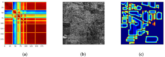
Figure 1. Data characteristics of the Indian Pines hyperspectral image: (a) Spectral band correlation matrix; (b) a noisy spectral band; and (c) spatial inhomogeneous pixel distribution.

In this paper, motivated by the idea of attention mechanisms, we construct a spatial–spectral squeeze-and-excitation (SSSE) structure to adaptively learn the weights for different spectral bands and for different neighboring pixels at the same time. SSSE can learn to train the network to suppress or motivate features at certain spectral bands or spatial positions, which can effectively overcome the redundancy in the spectral channels and the pixel inconsistency in the spatial neighborhood. Furthermore, we embed several SSSE modules into a residual network architecture and generate an SSSE based-residual network (SSSERN) model for HSI classification.

The rest of this paper is organized as follows. Section 2 introduces the residual network and SE structure, and then describes our proposed method. The experimental results and analysis are provided in Section 3. Section 4 gives a discussion. Finally, Section 5 draws the conclusions.

2. Spatial-Spectral Squeeze-and-Excitation Residual Network

For spectral-based classifiers, hundreds of spectral bands in the hyperspectral data will lead to a large degree of feature redundancy and noise, which dramatically affects the classification performance; especially when the number of training samples is small. For the spatial-neighborhood-based classification methods, neighboring pixels which are too far from the center pixel usually provide limited contributions to the classification of the central target pixel, especially when the neighborhood window is large. To overcome the redundancy in the spectral channels and the pixel inconsistency in the spatial neighborhoods, we propose a spatial–spectral squeeze-and-excitation (SSSE) structure, which can adaptively learn the weights for different spectral bands and for different neighboring pixels at the same time. Motivated by the idea of recalibration of the SE structure, the SSSE trains the network to suppress or motivate features at a certain position, which can effectively resist noise interference and improve the classification result.

2.1. Residual Connections

It has been demonstrated, in previous studies, that skip-connections can take advantage of the multi-level features of a CNN and are effective for various visual tasks [29,30,31,32]. Here, we briefly introduce the concept of residual connectivity [31,32]. A residual connection adds a shortcut by identity mapping, forcing the network to learn the residual function to restore the original non-linear transformation. The residual connection can be obtained by the following formula:

$$\begin{array}{c}\hfill {\mathit{X}}^l=h\left({\mathit{X}}^{l-1}\right)=f\left({\mathit{X}}^{l-1}\right)+{\mathit{X}}^{l-1},\end{array}$$

(1)

where ${\mathit{X}}^{l-1}$ and ${\mathit{X}}^l$ refer to the input and output of the l-th layer, and $h(·)$ is the original mapping. The desired underlying mapping h can be recovered by training the residual function $f(·)$ indirectly, which can be a composite transformation of conventional CNN operations. A typical residual module structure, called a bottleneck residual block, is shown in Figure 2.

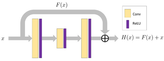
Figure 2. Schema of residual connections.

Residual connections can effectively enhance the flow of information between the top and bottom of the network and can alleviate the over-fitting problem. In addition, the extra mapping structure almost does not increase the parameter consumption of the network, and the residual networks are easier to optimize [30].

2.2. SpectralSE: Squeeze Spatial Information and Excite Spectral Features

In order to deal with hyperspectral images, we define a SpectralSE structure which squeezes spatial information and excites spectral features. Similar to the traditional squeeze-and-excitation (SE) module [28], SpectralSE aims to recalibrate the channel-wise feature responses by modelling interdependencies between the channels. Let $\mathbf{U}=\left[{\mathit{u}}_1,{\mathit{u}}_2,\cdots ,{\mathit{u}}_C\right]$ denote the input of the SE module, where ${\mathit{u}}_k\in {\mathbb{R}}^{H\times W}$ is the feature map of the k-th channel. As each element in ${\mathit{u}}_k$ corresponds to only one local area, this blind defect will result in a severe lack of global information in the bottom layer, with a less-receptive field [28]. In order to alleviate this problem, we propose to squeeze the global spatial information into a channel descriptor. This is achieved by using the global average operation over the spatial dimension, which generates a channel-wise statistic $\mathit{z}\in {\mathbb{R}}^C$, with elements

$$\begin{array}{c}\hfill z_k={\mathbf{F}}_{sq}\left({\mathit{u}}_k\right)=\frac{1}{H\times W}\sum _{i=1}^H\sum _{j=1}^W{\mathit{u}}_k(i,j),k=1,\cdots ,C,\end{array}$$

(2)

where ${\mathbf{F}}_{sq}(·)$ is called the squeeze operator.

To fully capture the channel-wise dependencies, in the process of excitation, a simple gating mechanism with a sigmoid activation $\sigma (·)$ is used to get the final stimulus value:

$$\begin{array}{c}\hfill \mathit{s}={\mathbf{F}}_{ex}(\mathbf{z},\mathbf{W})=\sigma \left({\mathit{W}}_1\left(\delta \left({\mathit{W}}_2\mathit{z}\right)\right)\right),\end{array}$$

(3)

where $\delta (·)$ is the ReLU function. In order to limit the complexity of the model, a bottleneck with two fully-connected (FC) layers is used to parameterize the excitation operation, and ${\mathit{W}}_1\in {\mathbb{R}}^{C\times \frac{C}{2}}$ and ${\mathit{W}}_2\in {\mathbb{R}}^{\frac{C}{2}\times C}$ are the weight matrices of the two fully-connected layers.

After the squeeze and excitation operations, the final output of the block is:

$$\begin{array}{c}\hfill {\mathbf{U}}_{SpectralSE}=\left[s_1{\mathit{u}}_1,s_2{\mathit{u}}_2,\cdots ,s_C{\mathit{u}}_C\right].\end{array}$$

(4)

Figure 3a depicts the schema of SpectralSE.

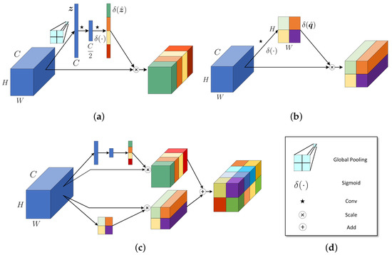
Figure 3. Mechanism of the proposed structure: (a) SpectralSE; (b) SpatialSE; (c) spatial–spectral squeeze-and-excitation (SSSE); and (d) key.

2.3. SpatialSE: Squeeze Spectral Information and Excite Spatial Features

Similar to SpectralSE, we also define a SpatialSE module, which transforms the dimensions of the SpectralSE operation from spectra to space. The feature maps of $\mathbf{U}$ are squeezed along the channel to compress the information of all channels. Then, we excite it and scale by the original spatial information. Let $\mathbf{U}=\left[{\mathit{u}}^{1,1},{\mathit{u}}^{1,2},\cdots ,{\mathit{u}}^{i,j},\cdots ,{\mathit{u}}^{W,H}\right]$ denote the slice on the spatial dimension, where ${\mathit{u}}^{i,j}\in {\mathbb{R}}^{1\times 1\times C}$ refers to the feature at the spatial position $(i,j)$. Squeeze and excitation operations are completed by performing the following convolution and sigmoid activation transformations:

$$\begin{array}{c}\hfill \mathit{q}={\mathbf{F}}_{ex}\left({\mathbf{F}}_{sq}\left(\mathbf{U}\right)\right)=\sigma (\mathit{W}\otimes \mathbf{U}),\end{array}$$

(5)

where $\mathit{W}\in {\mathbb{R}}^{1\times 1\times C}$ and $\mathit{q}\in {\mathbb{R}}^{W\times H}$. Each ${\mathit{q}}^{i,j}$ refers to an excited linear combination of all channels of U at position $(i,j)$.

The final recalibration result is obtained by multiplying $\mathbf{U}$ with the activation value:

$$\begin{array}{c}\hfill {\mathbf{U}}_{SpatialSE}=\left[{\mathit{q}}^{1,1}{\mathit{u}}^{1,1},\cdots ,{\mathit{q}}^{i,j}{\mathit{u}}^{i,j},\cdots ,{\mathit{q}}^{H,W}{\mathit{u}}^{H,W}\right].\end{array}$$

(6)

Figure 3b shows the framework of the SpatialSE module.

2.4. SSSE: Combination of SpectralSE and SpatialSE

Finally, we combine the spectralSE and SpatialSE modules to get the spatial–spectral squeeze-and-excitation (SSSE) structure:

$$\begin{array}{c}\hfill {\mathbf{U}}_{SSSE}=\alpha ·{\mathbf{U}}_{SpectralSE}+(1-\alpha )·{\mathbf{U}}_{SpatialSE},\end{array}$$

(7)

where $\alpha$ is a trainable variable, allowing the network to learn the proportions of channel excitation and spatial excitation, respectively. When the value at position $(i,j,c)$ in U is highly important, it will have a high activation value in the recalibration of the channel dimension and the spatial dimension. This recalibration encourages the network to learn more meaningful feature maps that are spectrally and spatially related. The SSSE structure is shown in Figure 3c.

2.5. SSSERN: Spatial-Spectral Squeeze-and-Excitation Residual Network

Now, we propose a new residual network that includes the SSSE structure, as shown in Figure 4. In the proposed SSSERN, batch normalization is used to correct the distribution of each layer and speed up the training [33]. The Xavier initialization method is used to initialize the network weights [34] and the Adam optimizer is used to minimize cross-entropy loss [35].

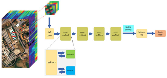
Figure 4. The procedure of the SSSE-based redisual network (SSSERN) method.

The details of the layers of the proposed SSSERN method are described in Table 1. The proposed network has four SSSE residual blocks. At the beginning, we use a $1\times 1$ convolution kernel to extract features. Taking the Indian Pines data set as an example, the hyperspectral cube with size $11\times 11\times 200$ is compressed to $11\times 11\times 128$ by performing convolution with 128 filters of size $1\times 1\times 200$. Here, the number of residual blocks and compression channels are adjustable. Following the SSSE residual blocks, a global pooling is used to transform the feature map into a one-dimensional vector. Finally, through softmax regression, the prediction labels corresponding to each category are obtained.

Table 1. Network architecture details of SSSERN for the Indian Pines Dataset.

Name	Details	Kernel Size
Input	-	-
Conv1	-	1, 1, 200, 128
SSSE-resBlock	resBlock	1, 1, 128, 32
		3, 3, 32, 32
		1, 1, 32, 128
	SpectralSE	128, 32
		32, 128
	SpatialSE	128, 1
⋯Repeat the Block 4 Times
Global pooling	-	-
Softmax Reg	-	128, 16

3. Experiments Results

3.1. Datasets

To evaluate the performance of the proposed method in HSI classification, we use the following two benchmark hyperspectral data sets:

(1) Indian Pines: This data was taken by the airborne visible/infrared imaging spectrometer (AVIRIS) sensor. The image scene contains $145\times 145$ pixels and 220 spectral bands, from 0.4–2.5 $\mathsf{\mu }$m, where 20 bands were discarded because of atmospheric affection. The spatial resolution of the Indian Pines data was 20 m. There are 16 classes in the data, as shown in Figure 5. The number of samples in each class is shown in Table 2.

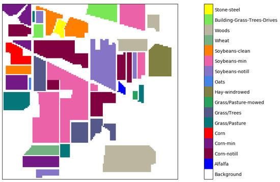
Figure 5. Color coding for the Indian Pines data set.

Table 2. Sample size for the Indian Pines scene.

Class		Samples
Number	Name	Number of Samples
1	Alfalfa	46
2	Corn-notill	1428
3	Corn-min	830
4	Corn	237
5	Grass/Pasture	483
6	Grass/Trees	730
7	Grass/Pasture-mowed	28
8	Hay-windrowed	478
9	Oats	20
10	Soybeans-notill	972
11	Soybeans-min	2455
12	Soybeans-clean	593
13	Wheat	205
14	Woods	1265
15	Building-Grass-Trees-Drives	386
16	Stone-steel Towers	93
Total		10,249

(2) University of Pavia: This data was acquired by the Reflective Optical System Imaging Spectrometer (ROSIS) sensor. The ROSIS sensor generates 115 bands, ranging from 0.43–0.86 $\mathsf{\mu }$m, in which 12 noisy bands were deleted and the remaining 103 bands are used for the experimental analysis. The spatial resolution is 1.3 m. The scene has the size of $610\times 340$, and contains 9 ground categories, as shown in Figure 6. The number of samples in each class is shown in Table 3.

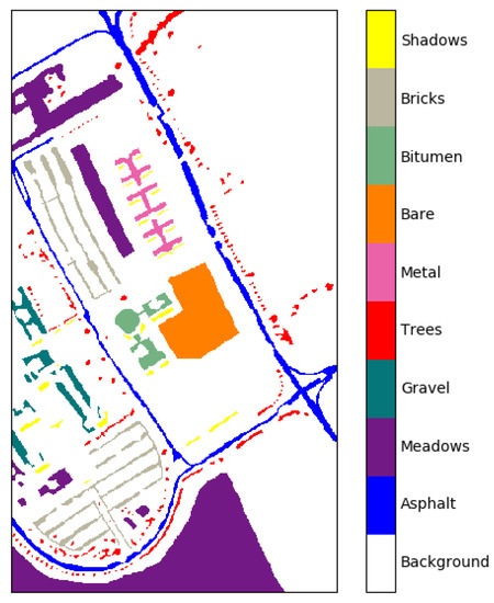
Figure 6. Color coding for the Pavia University data set.

Table 3. Sample size for the Pavia University scene.

Class		Samples
Number	Name	Number of Samples
1	Asphalt	6631
2	Meadows	18,649
3	Gravel	2099
4	Trees	3064
5	Metal sheets	1345
6	Bare soil	5029
7	Bitumen	1330
8	Bricks	3682
9	Shadows	947
Total		42,776

3.2. Classification Performance on Indian Pines and University of Pavia Data Sets

In this paper, the TensorFlow deep learning framework was used to build and train the proposed SSSERN. We compare the proposed method with six available classification methods in the literature: (1) Support Vector Machine (SVM) with a radial basis function kernel; (2) Random Forest (RF); (3) Multi-Layer Perceptron (MLP); (4) 2D-CNN [25]; (5) 3D-CNN [12]; and (6) SSRN [29]. Among these methods, SVM, RF, and MLP are spectral classifiers, and 2D-CNN can be considered as a spatial method which uses PCA to reduce the dimensionality of hyperspectral data and extracts only one principal component. Finally, 3D-CNN, SSRN, and the proposed SSSERN are spatial–spectral methods.

In the experiments, we randomly selected 15% samples from each class to form the training set and the test set consisted of the remaining samples. The experiment was repeated five times with randomly-chosen training samples, and the results of five runs were averaged. The class accuracy (CA), overall accuracy (OA), average accuracy (AA), and kappa coefficient ($\kappa$) on the testing set were recorded to assess the performance of the different classification methods. In 2D-CNN, 3D-CNN, and our proposed algorithm, the neighborhood window was set as $11\times 11$. The classification results on the two data sets are shown in Table 4 and Table 5, respectively.

Table 4. Overall, average, and individual class accuracies and $\kappa$ statistics in the form of mean ± standard deviation for the Indian Pines data set. The best results are highlighted in bold typeface.

Class	SVM	RF	MLP	2D-CNN	3D-CNN	SSRN	SSSERN
1	85.19 ± 3.02	73.15 ± 9.26	83.76 ± 9.00	70.94 ± 10.68	95.14 ± 7.98	97.53 ± 1.39	98.12 ± 0.97
2	82.68 ± 0.78	73.22 ± 1.74	71.78 ± 5.63	73.40 ± 3.19	96.96 ± 1.58	98.45 ± 0.26	99.63 ± 0.56
3	71.53 ± 2.21	72.13 ± 2.21	69.93 ± 1.13	74.85 ± 0.94	97.05 ± 1.90	97.70 ± 0.33	99.57 ± 0.54
4	65.67 ± 5.28	69.01 ± 5.98	74.96 ± 2.74	88.56 ± 5.24	89.68 ± 2.46	89.46 ± 2.78	99.41 ± 0.72
5	94.03 ± 1.53	90.92 ± 1.28	88.94 ± 2.03	69.35 ± 1.49	96.95 ± 1.65	99.16 ± 0.54	100.00 ± 0.00
6	97.54 ± 0.88	97.43 ± 0.51	94.89 ± 2.28	92.10 ± 3.52	98.71 ± 1.02	99.80 ± 0.29	99.74 ± 0.28
7	82.81 ± 9.38	73.44 ± 16.44	94.20 ± 2.51	65.22 ± 15.06	97.73 ± 4.55	100.00 ± 0.00	100.00 ± 0.00
8	98.08 ± 1.29	99.13 ± 0.45	97.29 ± 2.26	97.29 ± 1.37	99.21 ± 1.25	99.80 ± 0.25	100.00 ± 0.00
9	70.45 ± 13.64	72.73 ± 7.42	75.00 ± 6.25	81.25 ± 12.50	78.57 ± 24.74	94.64 ± 6.84	100.00 ± 0.00
10	73.20 ± 2.58	79.89 ± 3.44	84.42 ± 1.10	77.12 ± 4.97	95.52 ± 1.41	96.75 ± 0.37	99.52 ± 0.77
11	80.79 ± 1.16	90.23 ± 1.13	86.31 ± 2.78	86.19 ± 1.05	97.33 ± 1.02	98.13 ± 0.23	99.85 ± 0.69
12	78.17 ± 1.53	76.34 ± 2.10	74.21 ± 6.15	74.27 ± 1.27	97.46 ± 4.10	99.00 ± 0.61	96.54 ± 0.68
13	97.54 ± 1.50	96.72 ± 1.50	97.32 ± 0.33	98.85 ± 0.57	100.00 ± 0.00	100.00 ± 0.00	97.45 ± 0.82
14	94.82 ± 1.34	96.17 ± 0.81	96.16 ± 1.11	94.82 ± 2.07	99.38 ± 0.09	99.23 ± 0.28	99.91 ± 0.13
15	73.38 ± 2.93	58.87 ± 2.94	58.43 ± 2.83	80.89 ± 13.29	90.18 ± 3.76	94.07 ± 2.26	100.00 ± 0.00
16	93.64 ± 3.48	88.18 ± 5.65	90.72 ± 1.46	76.62 ± 4.10	89.73 ± 7.46	88.36 ± 4.26	95.94 ± 0.63
OA	83.61 ± 0.69	84.59 ± 0.55	83.48 ± 0.33	82.98 ± 0.78	97.01 ± 1.29	98.07 ± 0.17	99.44 ± 0.14
AA	83.72 ± 0.31	81.72 ± 1.24	83.64 ± 0.61	80.95 ± 1.54	96.98 ± 1.95	97.07 ± 0.68	98.89 ± 0.11
$\kappa$	81.29 ± 0.79	82.31 ± 0.63	81.09 ± 0.41	80.54 ± 0.90	96.59 ± 1.47	97.79 ± 0.19	99.03 ± 0.21

Table 5. Overall, average, and individual class accuracies and $\kappa$ statistics in the form of mean ± standard deviation for the University of Pavia data set. The best results are highlighted in bold typeface.

Class	SVM	RF	MLP	2D-CNN	3D-CNN	SSRN	SSSERN
1	90.72 ± 0.69	89.45 ± 0.01	89.91 ± 1.09	91.83 ± 0.33	99.10 ± 0.49	99.74  ± 0.11	100.00 ± 0.00
2	94.42 ± 0.63	97.83 ± 0.27	96.67 ± 0.75	97.11 ± 0.99	98.29 ± 0.68	99.35  ± 0.37	100.00 ± 0.00
3	70.34 ± 0.93	64.65 ± 0.83	79.32 ± 1.05	89.46 ± 0.68	90.01 ± 0.35	97.50  ± 0.50	98.39 ± 0.31
4	92.20 ± 0.56	90.52 ± 0.90	91.54 ± 0.58	91.89 ± 1.08	94.58 ± 0.16	98.68  ± 0.09	98.38 ± 0.11
5	98.87 ± 0.97	98.94 ± 0.89	98.87 ± 0.72	97.45 ± 0.70	100.00 ± 0.00	100.00 ± 0.00	100.00 ± 0.00
6	57.71 ± 0.78	63.39 ± 2.77	77.85 ± 1.09	68.09 ± 0.76	97.06 ± 0.26	98.50  ± 0.26	100.00 ± 0.00
7	77.73 ± 0.85	70.33 ± 0.97	81.77 ± 0.88	96.14 ± 0.74	89.54 ± 0.46	98.61  ± 0.18	99.74 ± 0.26
8	80.44 ± 0.69	86.36 ± 0.45	78.70 ± 0.98	95.27 ± 0.29	90.25 ± 0.28	95.76  ± 0.44	99.43 ± 0.35
9	92.39 ± 0.80	92.05 ± 0.51	93.87 ± 0.82	86.16 ± 0.14	99.51 ± 0.46	99.81  ± 0.54	96.19 ± 0.89
OA	86.17 ± 0.93	87.59 ± 0.35	90.64 ± 0.11	92.20 ± 0.16	96.59 ± 0.52	98.79  ± 0.26	99.62 ± 0.31
AA	83.78 ± 0.73	83.48 ± 0.21	87.61 ± 0.17	90.96 ± 0.70	95.12 ± 0.09	98.58  ± 0.26	99.13 ± 0.19
$\kappa$	81.63 ± 0.60	83.91 ± 0.33	87.36 ± 0.07	89.79 ± 1.02	95.37 ± 0.39	98.76  ± 0.54	99.35 ± 0.32

From the classification results, we can see that:

(1) The proposed SSSERN provided the best classification results on the two data sets.

(2) By jointly using the spectral and spatial information in a deep network architecture, the spatial–spectral methods (i.e., 3D-CNN, SSRN, and the proposed SSSERN) dramatically improved the spectral-based and spatial-based methods.

(3) Compared with existing deep learning methods (i.e., 2D-CNN, 3D-CNN and SSRN), the proposed SSSERN showed better results. This demonstrates that the proposed SSSE structure can extract much more effective spectral–spatial features by highlighting important spectral bands or neighboring pixels and suppressing noisy spectral bands or dissimilar neighboring pixels.

Figure 7 and Figure 8 show the classification maps of SVM, RF, MLP, 2D-CNN, 3D-CNN, SSRN, and our proposed SSSERN on the Indian Pines and University of Pavia data sets, respectively. The spectral-based classifiers, such as SVM and RF, generated noisy classification maps because they only considered isolated spectral samples and did not use spatial information to enhance the spatial neighborhood consistency. The spatial–spectral classifiers (i.e., 3D-CNN, SSRN, and SSSERN) provided much better results than the spectral classifiers and generated maps with little noise and clear object boundaries. Among all methods, our proposed SSSERN achieved a classification map that was the closest to the actual ground-truth; that is to say, the class boundaries were better defined and the background pixels were better classified.

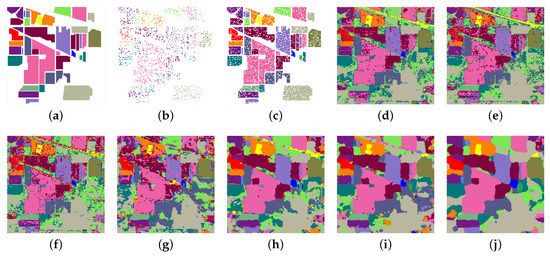
Figure 7. Classification maps for the Indian Pines data set. (a) Ground-truth. (b) Training set. (c) Testing set. Classification maps by: (d) SVM (83.77%); (e) RF (78.41%); (f) MLP (83.02%); (g) 2D-CNN (82.35%); (h) 3D-CNN (97.82%); (i) SSRN (98.09%); (j) SSSERN (99.45%).

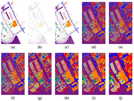
Figure 8. Classification maps for the University of Pavia data set. (a) Ground-truth; (b) training set; and (c) testing set. Classification maps by: (d) SVM (87.14%); (e) RF (88.15%); (f) MLP (90.71%); (g) 2D-CNN (92.65%); (h) 3D-CNN (97.01%); (i) SSRN (99.27%); and (j) SSSERN (99.70%).

3.3. Investigation on the Effect of Network Parameters

Now, we investigate the effect of parameters on the classification performance of SSSERN. The parameters are the width of input feature window $\omega$ (i.e., $\omega \times \omega$ is the window), the combination coefficient $\alpha$, and the number of residual blocks $N_{block}$, where $\omega$ controls the size of the input features, $\alpha$ is used to indicate the ratio of SpatialSE to SpectralSE, and $N_{block}$ decides the deepness of the network. We also investigate the effect of the number of training samples, where 5% and 15% samples from each class in Indian Pines are chosen for training.

We first fix $\alpha =0.5$ and $N_{block}=4$, and show the effect of $\omega$. Six different values of $\omega$ (3, 5, 7, 9, 11, and 13) were considered. The corresponding OA values of SSSERN, in the case of 5% and 15% training samples, are shown in Figure 9. It can be clearly seen that the OA of SSSERN increased rapidly with the increase of $\omega$ and achieved relatively stable results when $\omega \ge 9$. The optimal values of $\omega$ were 9 and 11 for 5% and 15% training samples, respectively. In the experiment, $\omega =11$ was used.

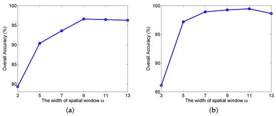
Figure 9. OA versus the width of the input feature window $\omega$: (a) 5% training samples; and (b) 15% training samples.

Next, we investigate the effect of $\alpha$. From Equation (7), when $\alpha =0$, the SSSE module is reduced to SpatialSE. When $\alpha =1$, SSSE is reduced to SpectralSE. When $\alpha =0.5$, SpatialSE and SpectralSE have the same importance in the SSSE. For simplicity, we only considered these three values of $\alpha$ (i.e., 0, 1, and 0.5). The OA of SSSERN versus different $\alpha$ values is shown in Figure 10, where SpectralSE, SpatialSE, and SSSE correspond to $\alpha =1$, $\alpha =0$, $\alpha =0.5$, respectively. It can be seen that the SSSE module that combined SpatialSE and SpectralSE provided the best results.

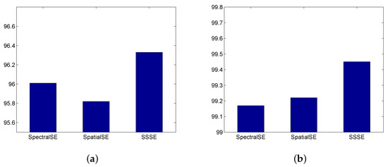
Figure 10. OA versus the combination coefficient $\alpha$: (a) 5% training samples; and (b) 15% training samples.

To further investigate the effectiveness of SSSE, we show the results of SSSERN with and without SSSE modules. As shown in Figure 4, the SSSE module is attached onto the residual block (resBlock). When the SSSE modules are deleted, SSSERN is reduced to a general residual network. Figure 11 shows the OA of SSSERN with and without SSSE modules. It can be clearly seen that SSSE modules were more effective than traditional residual modules, and the optimal number of SSSE blocks was either 3 or 4.

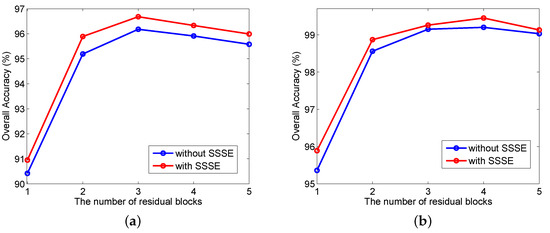
Figure 11. OA versus the number of SSSE residual modules: (a) 5% training samples; and (b) 15% training samples.

3.4. Investigation on the Stimulus Values by the SSSE Structure

Although previous experiments have proven the effectiveness of SSSE blocks in improving the network performance, we also want to understand how the automatic gating incentive mechanism works in practice. In this subsection, to show the behavior of the SSSE structure more clearly, we will study the activation outputs of individual samples in the model and check their distribution for different classes on different residual modules. Specifically, we choose six different classes from the Indian Pines data set (Classes 1, 3, 4, 11, 14, and 15), and select 50 samples from each class, and then calculate the average of the SSSE module output of these samples in different layers.

As the activation value in the SSSE structure is composed of two parts—namely, the stimulus value in the spectral and spatial dimensions—the visualization results of these two parts will be shown below. Figure 12 shows the averaged spectral dimension stimulus value for each class. It can be seen that different classes of samples had different stimulus values for each channel, in each SSSE structure. In the third SSSE structure, Classes 1, 3, 4, and 14 showed synchronization suppression effects at the 36th channel, which demonstrates that the spectral characteristics of these classes were similar in this channel.

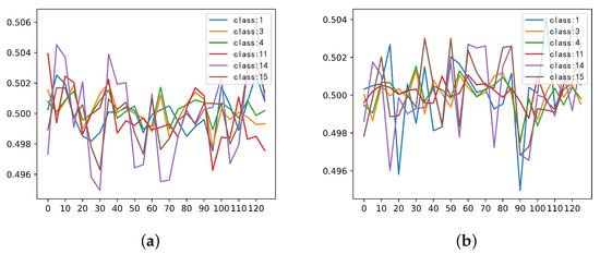
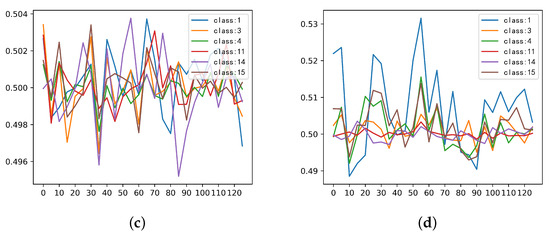
Figure 12. Averaged spectral dimension stimulus value for the six classes in different SpectralSE blocks: (a) SpectralSE 1; (b) SpectralSE 2; (c) SpectralSE 3; and (d) SpectralSE 4.

Figure 13 shows the activation values of the six classes in the spatial dimensions of different SSSE layers. In the figure, the brighter part corresponds to higher activation values. It can be seen that the features were almost always activated at the center position, and the positions around the boundary were suppressed. The boundary pixels may have been background pixels or pixels from different classes for a large window. In addition, they were far away from the central pixel and, hence, were less important. By suppressing these boundary pixels, the SSSERN model can obtain better results.

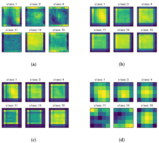
Figure 13. Averaged spatial dimension stimulus value for the six classes in different SpatialSE blocks: (a) SpatialSE 1; (b) SpatialSE 2; (c) SpatialSE 3; and (d) SpatialSE 4.

4. Discussion

The SSSE structure can re-calibrate the spatial and spectral features by using learning methods and has achieved the purpose of suppressing or stimulating certain features related to classification. In the following, we will provide an example to display the effect of SSSE. Given a pixel from Class 11 of the Indian Pines data set, we can construct an $11\times 11$ spatial neighborhood, as shown in Figure 14. It is clear that the neighborhood contains background pixels with label 0, and pixels from the same class 11, and from the (different) classes 5 and 6. We compute the simulation value of the first layer SpatialSE structure, corresponding to the pixels in the neighborhood, and show the simulation values as different colors in Figure 14. The brighter or darker colors correspond to larger or smaller excitation values. It can be clearly seen that SpatialSE can generate a mask to stimulate the homogeneous pixels which are helpful for classification and, meanwhile, suppress inhomogeneous pixels (i.e., background pixels and pixels from classes 5 and 6) which have negative effects on the classification.

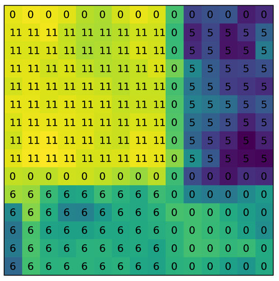
Figure 14. The first-layer SpatialSE simulation value for an $11\times 11$ spatial neighborhood.

5. Conclusions

In this paper, we have proposed a spatial–spectral squeeze-and-excitation residual network (SSSERN) method for HSI classification. In the framework of a residual network, the proposed SSSERN contains four SSSE blocks, which can excite or suppress features in the spectral and spatial dimensions, simultaneously, by feature re-calibration. The proposed SSSERN is compared with some state-of-the-art deep learning methods. The experimental results on the Indian Pines and University of Pavia data sets have shown the effectiveness of SSSERN.

References

- Landgrebe, D. Hyperspectral image data analysis. IEEE Signal Process. Mag. 2002, 19, 17–28. [Google Scholar] [CrossRef]
- Fauvel, M.; Tarabalka, Y.; Benediktsson, J.A.; Chanussot, J.; Tilton, J.C. Advances in spectral-spatial classification of hyperspectral images. Proc. IEEE 2013, 101, 652–675. [Google Scholar] [CrossRef]
- Bioucas-Dias, J.M.; Plaza, A.; Camps-Valls, G.; Scheunders, P.; Nasrabadi, N.; Chanussot, J. Hyperspectral remote sensing data analysis and future challenges. IEEE Geosci. Remote. Sens. Mag. 2013, 1, 6–36. [Google Scholar] [CrossRef]
- Wang, Q.; Meng, Z.; Li, X. Locality adaptive discriminant analysis for spectral-spatial classification of hyperspectral images. IEEE Geosci. Remote. Sens. Lett. 2017, 14, 2077–2081. [Google Scholar] [CrossRef]
- Donoho, D.L. High-dimensional data analysis: The curses and blessings of dimensionality. AMS Math Chall. Lect. 2000, 1, 32. [Google Scholar]
- Huang, Z.; Zhu, H.; Zhou, T.; Peng, X. Multiple marginal fisher analysis. IEEE Trans. Ind. Electron. 2018. [Google Scholar] [CrossRef]
- Zhou, Y.; Peng, J.; Chen, C.L.P. Dimension reduction using spatial and spectral regularized local discriminant embedding for hyperspectral image classification. IEEE Trans. Geosci. Remote. Sens. 2015, 53, 1082–1095. [Google Scholar] [CrossRef]
- He, L.; Li, J.; Liu, C.; Li, S. Recent advances on spectral-spatial hyperspectral image classification: An overview and new guidelines. IEEE Trans. Geosci. Remote. Sens. 2018, 56, 1579–1597. [Google Scholar] [CrossRef]
- Zhou, Y.; Peng, J.; Chen, C.L.P. Extreme learning machine with composite kernels for hyperspectral image classification. IEEE J. Sel. Top. Appl. Earth Obs. Remote. Sens. 2015, 8, 2351–2360. [Google Scholar] [CrossRef]
- Peng, J.; Zhou, Y.; Chen, C.L.P. Region-kernel-based support vector machines for hyperspectral image classification. IEEE Trans. Geosci. Remote. Sens. 2015, 53, 4810–4824. [Google Scholar] [CrossRef]
- Peng, J.; Du, Q. Robust joint sparse representation based on maximum correntropy criterion for hyperspectral image classification. IEEE Trans. Geosci. Remote. Sens. 2017, 55, 7152–7164. [Google Scholar] [CrossRef]
- Chen, Y.; Lin, Z.; Zhao, X.; Wang, G.; Gu, Y. Deep learning-based classification of hyperspectral data. IEEE J. Sel. Top. Appl. Earth Obs. Remote. Sens. 2014, 7, 2094–2107. [Google Scholar] [CrossRef]
- Hu, F.; Xia, G.; Hu, J.; Zhang, L. Transferring deep convolutional neural networks for the scene classification of high-resolution remote sensing imagery. Remote Sens. 2015, 7, 14680–14707. [Google Scholar] [CrossRef]
- Zhang, L.; Zhang, L.; Du, B. Deep learning for remote sensing data: A technical tutorial on the state of the art. IEEE Geosci. Remote. Sens. Mag. 2016, 4, 22–40. [Google Scholar] [CrossRef]
- Zhu, X.; Tuia, D.; Mou, L.; Xia, G.; Zhang, L.; Xu, F.; Fraundorfer, F. Deep learning in remote sensing: A comprehensive review and list of resources. IEEE Geosci. Remote. Sens. Mag. 2017, 5, 8–36. [Google Scholar] [CrossRef]
- Zhao, C.; Wan, X.; Zhao, G.; Cui, B.; Liu, W.; Qi, B. Spectral-spatial classification of hyperspectral imagery based on stacked sparse autoencoder and random forest. Eur. J. Remote. Sens. 2017, 50, 47–63. [Google Scholar] [CrossRef]
- Li, T.; Zhang, J.; Zhang, Y. Classification of hyperspectral image based on deep belief networks. In Proceedings of the 2014 IEEE International Conference on Image Processing, Paris, France, 27–30 October 2014; pp. 5132–5136. [Google Scholar]
- Zhong, P.; Gong, Z.; Li, S.; Schnlieb, C. Learning to diversify deep belief networks for hyperspectral image classification. IEEE Trans. Geosci. Remote. Sens. 2017, 55, 3516–3530. [Google Scholar] [CrossRef]
- Chen, Y.; Jiang, H.; Li, C.; Jia, X.; Ghamisi, P. Deep feature extraction and classification of hyperspectral images based on convolutional neural networks. IEEE Trans. Geosci. Remote. Sens. 2016, 54, 6232–6251. [Google Scholar] [CrossRef]
- Lecun, Y.; Bengio, Y.; Hinton, G. Deep learning. Nature 2015, 521, 1476–4687. [Google Scholar] [CrossRef] [PubMed]
- Wang, Q.; Gao, J.; Yuan, Y. Embedding structured contour and location prior in siamesed fully convolutional networks for road detection. IEEE Trans. Intell. Transp. Syst. 2018, 19, 230–241. [Google Scholar] [CrossRef]
- Peng, X.; Feng, J.; Xiao, S.; Yau, W.; Zhou, T.; Yang, S. Structured autoEncoders for aubspace clustering. IEEE Trans. Image Process. 2018, 27, 5076–5086. [Google Scholar] [CrossRef] [PubMed]
- Mei, S.; Ji, J.; Bi, Q.; Hou, J.; Du, Q.; Li, W. Integrating spectral and spatial information into deep convolutional neural networks for hyperspectral classification. In Proceedings of the 2016 IEEE International Geoscience and Remote Sensing Symposium, Beijing, China, 10–15 July 2016; pp. 5067–5070. [Google Scholar]
- Yang, J.; Zhao, Y.; Chan, J.C.; Yi, C. Hyperspectral image classification using two-channel deep convolutional neural network. In Proceedings of the 2016 IEEE International Geoscience and Remote Sensing Symposium, Beijing, China, 10–15 July 2016; pp. 5079–5082. [Google Scholar]
- Zhang, H.; Li, Y.; Zhang, Y.; Shen, Q. Spectral-spatial classification of hyperspectral imagery using a dual-channel convolutional neural network. Remote Sens. Lett. 2017, 8, 438–447. [Google Scholar] [CrossRef]
- Li, Y.; Zhang, H.; Shen, Q. Spectral-spatial classification of hyperspectral imagery with 3D convolutional neural network. Remote Sens. 2017, 9, 67. [Google Scholar] [CrossRef]
- Paoletti, M.E.; Haut, J.M.; Plaza, J.; Plaza, A. A new deep convolutional neural network for fast hyperspectral image classification. ISPRS J. Photogramm. Remote. Sens. 2018, 145, 120–147. [Google Scholar] [CrossRef]
- Hu, J.; Shen, L.; Sun, G. Squeeze-and-excitation networks. In Proceedings of the IEEE Conference on Computer Vision and Pattern Recognition, Salt Lake City, Salt Lake City, UT, USA, 18–22 June 2018; pp. 7132–7141. [Google Scholar]
- Zhong, Z.; Li, J.; Luo, Z.; Chapman, M. Spectral-spatial residual network for hyperspectral image classification: A 3-D deep learning framework. IEEE Trans. Geosci. Remote. Sens. 2018, 56, 847–858. [Google Scholar] [CrossRef]
- He, K.; Zhang, X.; Ren, S.; Sun, J. Deep residual learning for image recognition. In Proceedings of the IEEE Conference on Computer Vision and Pattern Recognition, Las Vegas, NV, USA, 27–30 June 2016; pp. 770–778. [Google Scholar]
- He, K.; Zhang, X.; Ren, S.; Sun, J. Delving deep into rectifiers: Surpassing human-level performance on imagenet classification. In Proceedings of the IEEE International Conference on Computer Vision, Santiago, Chile, 7–13 December 2015; pp. 1026–1034. [Google Scholar]
- He, K.; Zhang, X.; Ren, S.; Sun, J. Identity mappings in deep residual networks. In Proceedings of the European Conference on Computer Vision, Amsterdam, The Netherlands, 8–16 October 2016; pp. 630–645. [Google Scholar]
- Ioffe, S.; Szegedy, C. Batch normalization: Accelerating deep network training by reducing internal covariate shift. arXiv, 2015; arXiv:1502.03167. [Google Scholar]
- Glorot, X.; Bordes, A.; Bengio, Y. Deep sparse rectifier neural networks. In Proceedings of the 14th International Conference on Artificial Intelligence and Statistics, Fort Lauderdale, FL, USA, 11–13 April 2011; pp. 315–323. [Google Scholar]
- Kingma, D.P.; Ba, J. Adam: A method for stochastic optimization. arXiv, 2014; arXiv:1412.6980. [Google Scholar]
© 2019 by the authors. Licensee MDPI, Basel, Switzerland. This article is an open access article distributed under the terms and conditions of the Creative Commons Attribution (CC BY) license (http://creativecommons.org/licenses/by/4.0/).