Review

Retrieving Sea Level and Freeboard in the Arctic: A Review of Current Radar Altimetry Methodologies and Future Perspectives

1
Plymouth Marine Laboratory, Prospect Place, The Hoe, Plymouth PL1 3DH, UK
2
Finnish Meteorological Institute, Erik Palménin aukio 1, FI-00560 Helsinki, Finland
3
Deutsches Geodätisches Forschungsinstitut, Technische Universität München, (DGFI-TUM), 80333 München, Germany
4
DTU Space, National Space Institute, Elektrovej Bygning 327, 2800 Kongens Lyngby, Denmark
5
He Space, Robert-Bosch-Strasse 7, 64293 Darmstadt, Germany
6
LEGOS, 4 Avenue Edouard Belin, 31400 Toulouse, France
7
Centre National d’Etudes Spatiales, 18 Avenue Edouard Belin, 31400 Toulouse, France
8
Alfred Wegener Institute, Am Handelshafen 12, 27570 Bremerhaven, Germany
9
Centre for Polar Observation and Modelling, Earth Sciences, University College London, 5, Gower Place, London WC1E 6BS, UK
*
Author to whom correspondence should be addressed.
Remote Sens. 2019, 11(7), 881; https://doi.org/10.3390/rs11070881
Submission received: 13 March 2019 / Revised: 4 April 2019 / Accepted: 9 April 2019 / Published: 11 April 2019
(This article belongs to the Special Issue Advances in Satellite Altimetry and Its Application)

Abstract

:
Spaceborne radar altimeters record echo waveforms over all Earth surfaces, but their interpretation and quantitative exploitation over the Arctic Ocean is particularly challenging. Radar returns may be from all ocean, all sea ice, or a mixture of the two, so the first task is the determination of which surface and then an interpretation of the signal to give range. Subsequently, corrections have to be applied for various surface and atmospheric effects before making a comparison with a reference level. This paper discusses the drivers for improved altimetry in the Arctic and then reviews the various approaches that have been used to achieve the initial classification and subsequent retracking over these diverse surfaces, showing examples from both LRM (low resolution mode) and SAR (synthetic aperture radar) altimeters. The review then discusses the issues concerning corrections, including the choices between using other remote-sensing measurements and using those from models or climatology. The paper finishes with some perspectives on future developments, incorporating secondary frequency, interferometric SAR and opportunities for fusion with measurements from laser altimetry or from the SMOS salinity sensor, and provides a full list of relevant abbreviations.

Graphical Abstract

1. Introduction

Within the Arctic Ocean, radar altimetry is used to monitor both the sea level and the freeboard of sea ice, i.e., how far the ice surface is above the surrounding water level. The sea level is a measure of the amount of water within a basin, but assuming the geostrophic approximation to be valid, its spatial derivative is also an indicator of surface currents. The freeboard is used to infer sea-ice thickness (SIT), which may be combined with sea-ice concentration (SIC), i.e., the areal fraction (as determined by passive microwave sensors) to give the volume of sea ice. Changes in this volume are then indicators of latent heat lost from the Arctic and of the amount of highly saline water produced through brine rejection. Thus, Arctic Ocean altimetry helps provide a number of measures for monitoring the environment, both for short-term responses to force and to understand the effects of climate change. This paper provides a review of the methodological techniques required to obtain useful environmental information from altimeters, giving an overview of the choice of approaches available to interested users. This paper does not explore the scientific results achieved because there has been a good recent summary of those by Johannessen and Andersen [1].

1.1. Scientific and Operational Requirements

The ice cover in the Arctic changes markedly in the course of a year [2]: as air temperatures drop from September onwards, heat loss from the water leads to ice formation first as pancake and frazil ice that are then aggregated to produce a near-continuous layer, which subsequently thickens and eventually breaks into pieces. These pieces, known as ice floes are flexed by waves and moved by winds and currents. A short-term divergence between neighbouring ice floes leads to the creation of a linear, narrow lead of ice free water, which will then freeze up, whereas offshore winds near a coast may lead to a more permanent open water feature known as a polynya. From roughly March onwards solar irradiation leads to melting and the formation of fresh water “melt ponds” on top of the ice, before complete thawing to produce low salinity surface water. The resultant stratification supports an immediate phytoplankton bloom [3]. At minimum sea-ice extent (in September) there is still much of the central Arctic that is ice-covered (see Figure 1b), but due to the continual ice drift the resultant multi-year ice (which has different physical properties to first-year ice) will occupy a different region to that of minimum ice extent, with new freshly-produced ice replacing it. Further details on the nomenclature of different ice types and features are provided by WMO [4].
The Arctic environment is changing dramatically, such that over the past 50 years, the Arctic has warmed more than twice as rapidly as the rest of the Earth [5]. Since February of last year (2018), the north of Greenland has been around 15 C warmer than average for this month, possibly retarding the thermodynamic ice growth in the polynya that opened due to the strong katabatic winds. Together with these clear atmospheric temperature changes, ocean temperatures are also increasing with a warming hotspot observed consistently over the last few autumns and winters in the Barents Sea [6,7], also contributing to the global sea level rise by thermal expansion. Other indicators of the changes occurring in the Arctic are the numerous records for the lowest sea-ice extent and thickness during the past years [8]. Despite a strong interannual variability, the sea-ice extent clearly continues a long-term downward trend [8]. By extrapolating the recent observations, we can predict a summer ice-free Arctic Ocean by the late 2030s [9,10], which is earlier than previously expected. These long-term changes affect the Arctic ecosystems and the weather in lower latitudes (e.g., extreme cold events in Europe and Southeast Asian monsoons) due to the modifications of atmospheric circulation [11].
To understand these issues of climate change, a number of different Earth Observation (EO) datasets are brought together: sea-ice area, concentration, drift, thickness as well as the topography of the ocean at global and regional scales. In climate change studies based on satellite data, it is a major challenge to construct homogeneous time series from consecutive satellite sensors, which are required for the detection of changes over several decades. This is the main goal of the Climate Change Initiative from European Space Agency (ESA), with projects both on the Sea Level [12,13] and on Sea Ice [14]. For climate studies, the sea level needs to be measured on a regional basis (using a grid mesh of size 50–100 km) to within 1 cm, with a stability of the measurement able to resolve any long-term trend to within 1 mm yr 1 [15]. Using non-altimetry data for 1954 to 1989, Proshutinsky et al. [16] estimated the sea level rise in the Russian sector of the Arctic to be 1.85 mm yr 1 after a global isostatic adjustment. These accuracy requirements are very challenging over the Arctic, knowing the geophysical correction uncertainties and the sparsity of sea level measurements in ice-infested areas. Larger amplitude changes are expected on a regional basis, e.g., in response to changes in the Arctic Ocean Oscillation [17]. Declassified submarine sonar data for part of the Arctic reveal that the ice thickness for that region has almost halved between 1979 and 2008 [18]. To address the issues concerning the sea ice’s response to polar warming, GCOS [15] proposed a target accuracy for sea ice thickness measurements of 10 cm, although acknowledging that the accuracy achievable at that time was approx. 50 cm when averaged over a month.
On the other hand, operational applications today require high-resolution products over the Arctic with a minimal time delay. The typical diameter of mesoscale eddies in the Arctic is less than 20 km [20], but the dominant circulation features (see Figure 1a) have a coherence along their flow, which aids in their monitoring. Modellers need the Arctic sea level and SIT products on a daily basis. The navigational requirements include products detailing ice-free time and zones, ice thickness, ice drift and snow on sea ice. There is a particular need for data along the main intended shipping routes, where the requirement is for the ice concentration, channel portion (open water portion that can be used for navigation), ridged ice fraction [21] and sizes for different ice types. For many of these parameters, thet daily evolutions and high spatial resolution are of great interest, but ship operators also need a long time series of the sea-ice thickness when planning operations in the Arctic. The Polar Code [22] requires manuals for ship operations to include considerations of the ice conditions in their planned area of operations, and altimeter SIT estimates can be used to complement other sources of information in this planning.
Improving our ability to project future sea-level rise and sea-ice conditions implies developments in both the observing systems (to constrain and validate the models with present and recent past observations) and the modelling of various processes at different spatial and temporal scales. Although significant progress has been made in the past decade, there are significant benefits in improving all the observing systems needed to measure and interpret sea-ice characterization and sea-level change as well as improving the modelling of future projections of ice melt and global sea-level rise and their regional impacts.

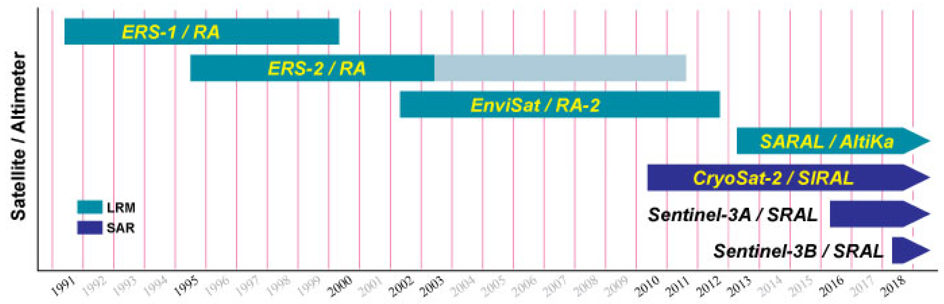
1.2. Relevant Altimeter Datasets

Altimeters provide nadir measurements of range, with a fine along-track spacing but with no swath coverage. This means that with a single altimeter, adequate spatial coverage is only achieved upon collating a pattern of different tracks spanning tens of days; therefore, the production of self-consistent maps of the sea level on a monthly basis requires an analysis and homogenization of the data from multiple altimeters (see Figure 1 of Quartly et al. [12]). For Arctic analyses, there is the complication that whilst there is a dense coverage at the satellite’s turning latitude (defined by its orbital inclination), there is no coverage beyond that. Since the chosen orbit for a satellite is a compromise with other mission demands, only a few altimeters have provided data north of 72 N (the limit for Geosat and Geosat Follow On).
ESA has launched a series of satellites (see Figure 2 and Table 1) into orbits with an inclination of approx. 98.5 , enabling coverage up to 81.5 N. These were ERS-1 (launched in 1991), ERS-2 (1996) and Envisat (2002), all with operations at Ku-band (13.6 GHz), with the principal differences being that Envisat had a higher pulse repetition frequency (PRF), enabling more independent pulses to be averaged in each 0.05 seconds, and had an additional frequency of operation, in S-band (3.2 GHz).
The ERS/Envisat 35-day orbit was adopted by SARAL/AltiKa, which is the only altimeter to eschew the Ku-band in favour of the Ka-band for operations [24]. This enables it to operate with shorter radio pulses and gives it a slightly smaller ground footprint than the equivalent Ku-band sensors and less sensitivity to delays by free electrons in the ionosphere. Radio waves at the Ka-band are much more affected by moisture in the troposphere than is the case for Ku-band, but this is not relevant for polar studies. Although all these instruments posted data at 20 Hz corresponding to approx. 330 m along the track, the size of their effective footprint is much larger, being “pulse-limited” (i.e., dependent upon the width of the emitted pulse), with values between 2 and 10 km in diameter depending upon wave height [23].
A major technological change from these “conventional” low-resolution measurement (LRM) sensors was the introduction of instruments with a delay-Doppler or SAR Measurement (SARM) processing capability. [The term “delay-Doppler altimeter” (DDA) describes the specific implementation used for Cryosat-2 and Sentinel-3, but the expression “SAR altimetry” is more commonly used, and this should not be confused with the 2-D radar images achieved by side-looking synthetic aperture radars.] For details on the technological advances, please consult Raney [25] and Wingham et al. [26]. This latter mode of operation enables a finer along-track resolution and lower noise levels due to the accumulation of looks (multi-looking) from multiple viewing geometries. The resultant radar echoes (“waveforms”) have a narrower shape (see Figure 3). Although their output can be degraded into a pseudo-LRM waveform and processed similarly to previous LRM instruments, it is preferable to develop new processing techniques to utilise the greater information content available in these SAR waveforms. This technology was first demonstrated by CryoSat-2 and has become more operational with Sentinel-3A and the recently-launched Sentinel-3B.
In the succeeding sections, we discuss first how these waveform data and derived fields are used to discriminate between different reflecting surfaces (principally open ocean, leads and floes) and then how these data are subsequently retracked, i.e., processed to give an accurate estimate of range.

2. Waveform Discrimination

It is important to be able to distinguish accurately between reflections from different surfaces (open ocean, floes and leads), as different stages of processing are usually applied to each surface type. This section reviews the methodologies available to achieve this discrimination. First, we consider waveforms from LRM instruments, detailing the classification approaches based on physically interpretable characteristics (Section 2.1.1), and then, we provide an overview of the key techniques implementing machine-learning (Section 2.1.2); Section 2.2 covers the equivalent ideas for SAR instruments. Section 2.3 then summarises the challenges and approaches to providing a quantitative validation of these classifications.

2.1. LRM Altimeters

Reflections from open ocean normally produce waveforms to which a smooth functional form can be fitted (see Figure 4a). For LRM echoes, the leading edge width (LEW) is related to the wave height, and the normalized backscatter, σ 0 , is related to the surface roughness [27,28], and the trailing edge slope (TES) is sometimes associated with the mispointing of the satellite [29]. The parameters LEW, TES and σ 0 are also relevant over sea-ice free from leads, although the waveform shape may be slightly different (Figure 3), and the backscatter from the ice will give a different range of σ 0 values. LRM waveforms over leads in the sea ice have a significantly different shape because the calm conditions within the lead to provide a mirror-like surface and, thus, high backscatter values. The specular reflections from such a surface mean that only points directly at nadir contribute significantly, so virtually all the power in the signal originates from a small area and is, thus, confined to a small number of waveform bins.

2.1.1. Classical Techniques

The simplest approaches to surface discrimination identify certain waveform characteristics which have significantly different values over disparate surfaces and use permitted ranges to assign the data to different classifications. Several of the parameters used are descriptors of the fitted waveform, e.g., LEW, TES and σ 0 , which are shown in Figure 4a. Various definitions of σ 0 may exist within the data stream according to which model is fitted. Another characteristic of the waveform is pulse peakiness ( P P ), which was introduced by Laxon [30] and is defined as the ratio of the peak power in any of the waveform bins to the mean power over those bins expected to hold the signal (i.e., from the leading edge onwards). There are variants as some users chose different integration ranges or normalization factors, but a generally-accepted implementation is included in modern GDRs (Geophysical Data Records). Zakharova et al. [31] note that there was a hard limit on the waveform counts for AltiKa of 1250 (see Figure 4b), affecting 6–10% of data. This limited the usefulness of P P for lead discrimination for that mission, especially as different settings for the AGC (Automatic Gain Control) would change the scaling of the waveform and, thus, the mean number of counts but not the maximum. Therefore, for the surface discrimination for AltiKa, they introduced a new term, the maximal waveform power ( M P ):
M P = 10 l o g 10 ( m a x ( P i ) ) + A G C
where P i is the power level in the ith waveform bin.
Although there are basic physical models governing the expected waveform shape over an open ocean and ice floes, the thresholds used in the classification tend to be chosen empirically by various research teams. Usually, the precise thresholds are not important; what limits the efficacy of the classification is whether the assumptions behind the evaluation are valid. Indeed, the distribution of values for PP depends upon the waveform shape (and thus on radar frequency) and on the number of pulses summed to generate an “average waveform”. The sea-ice processing chain at University College London (UCL) has used P P and σ 0 , with additional contextual information from daily composites of the sea-ice concentration (SIC) from passive microwave satellites. From this, they generated the first pan-Arctic view of the sea-ice thickness from ERS-1 and ERS-2 [32] and the first accurate mean sea surface for the Arctic [33]. The “multiple criteria” approach used by Poisson et al. [34] also included some constraints on P P , L E W and σ 0 . For AltiKa, Zakharova et al. [31] used M P , which is akin to a combination of peakiness and σ 0 (as the AGC setting is the altimeter’s delayed on-board response to changes in σ 0 ).

2.1.2. Statistical Techniques

In the preceding section, the waveform classification was based on simple thresholds for various criteria, with those bounds set by the user on the basis of physical insight and empirical interpretation of histograms of those parameters. Further classification approaches are developed that adopt machine-learning techniques and data-mining strategies, such as partitional clustering methods like K-Means or Neural Networks (NN). Previous studies [34,35,36,37,38] used fixed thresholds for the echo assignment; machine-learning classification strategies are characterized by a high flexibility and dynamic adaption to various surface characteristics. An analysis by Dettmering et al. [39] compares different classification strategies based on CryoSat-2 waveforms and points out their benefits and advantages. The algorithms are used to assign the received radar echoes based on pattern recognition, by analysing similarities and differences among the waveform data, without being limited to a certain satellite altimetry mission or specific surface conditions. The statistical approaches are divided into (i) supervised classification algorithms, which require already classified training datasets (e.g., NN) in order to link received waveforms on the basis of predefined characteristics for specific surface types, and (ii) unsupervised classification algorithms (e.g., partitional clustering), which perform a waveform assignment without pre-classified radar echoes. The present paper provides one example for each of these approaches.
Müller et al. [37] produced a clustering algorithm that used six waveform features in an unsupervised classification (i.e., a system in which there no predefined target groupings). For this, they needed a reference dataset comprising the majority of all possible scatter types. The partitioning of data is achieved using the K-medoids clustering algorithm, which categorizes waveforms into a predefined number of K classes. Figure 5 shows the separation of more than 300,000 Envisat waveforms into 30 classes. These clusters are then assigned to different surface conditions in order to condense them to “ocean”, “ice floe” and “lead/polynya” returns. This is achieved by analysing the mean feature values of each cluster and comparing the selected exemplary waveforms with the SAR data (see Section 2.3.2). For example, clusters displaying very narrow and clear single-peaked waveforms (e.g., cluster numbers 2, 10, 11, 12, 20 and 26) are assigned to the lead/polynya clusters. Waveforms exhibiting a typical ocean-like shape, characterized amongst other aspects by a weak trailing edge slope or decreased maximum power value, (e.g., clusters 1, 3, 6 and 25) are allocated to ocean waveforms. The remaining clusters represent ice returns. If there is no clearly interpretable signature, then they are set to “undefined” (e.g., clusters 4 and 15). Afterwards, the obtained waveform model is used to classify and label all remaining waveforms. This is done by the K-nearest neighbour, which is a memory-based classifier method.
Another possible classification method is based on the use of a Neural Network (NN), as described in Gommenginger et al. [38] and Poisson et al. [34]. This approach is a supervised classification, i.e., the neural net is trained to associate particular waveform shapes with user-specified classes (Figure 6). Again the input data is not the full set of waveform bins but a small set of characteristics describing the shape and amplitude of the waveform, which include P P , TES and LEW, as well as the existence or not of extra peaks in the trailing edge. Neural network classifiers directly model discriminant functions (functions enabling the prediction of the group membership of a sample based on the values of the input predictive variables) if the output values are defined in an appropriate way. It requires a large training dataset with enough representative examples of each of the predefined classes.
The purpose is to classify the different geometrical shapes of the echoes (see Figure 6) and not the different surfaces, even if some links can be made between them. It is important to define the classes not only for all echo shapes of interest but also for all other waveforms numerous enough to impact the classifier. Even if they do not provide useful information, their identification as a dedicated class number prevents the algorithm from misclassifying them as shapes of interest. Poisson et al. [34] used 12 classes to cover all possible Envisat waveforms in the Arctic, with one of those corresponding to “ocean”, one to “leads” and three of them subsequently amalgamated to specify “floes”. The remaining classes were deemed too complex for further interpretation and retracking. This method has been expanded to also work with waveforms from AltiKa and Sentinel-3 [40].

2.2. SAR Altimeters

In SAR altimetry, the information telemetered to the ground station can be used to infer the time delay and the Doppler shift of the echoes. Whilst the time delay indicates, as for LRM, which annulus about the nadir point is contributing, the Doppler shift gives the position fore or aft of the satellite flight direction; together, these give a much finer resolution cell [25]. A SAR altimeter, thus, provides a multi-look viewing for each sub-satellite point; the range correction then aligns these multiple records for a given point within a “waveform stack” (Figure 4c,f). An incoherent sum over all look directions gives a SAR waveform (Figure 4e), which is sharper than an LRM waveform because of the finer footprint achieved through Doppler processing, and has a lower noise level due to the higher number of pulses averaged. Alternatively, the stack may be summed in the orthogonal direction to give the Range Integrated Power (RIP, see Figure 4d).
Both waveforms and RIP will be peaky when the satellite moves over a very smooth surface, such as a lead. For open sea and ice, i.e., for areas in which the scatterers have different orientations (diffuse scattering of rough surfaces), the RIP will be closer to a Gaussian shape, with a much larger value for the SSD (Stack Standard Deviation). The Stack Skewness (SS) and Stack Kurtosis (SK) are the other characteristics calculated from the RIP and provided within the GDRs. Because of its finer along-track resolution, SAR altimetry, therefore, has the potential to provide sea-ice observations closer to the edge of leads. Nevertheless, waveforms returned over a floe may still be strongly affected by bright reflections from off-nadir leads, especially those to the side of the track.
The current research on SAR waveform discrimination can be divided into three main techniques, which are described below.

2.2.1. Power-Based Methods

Power-based methods build on the assumption that the smoother the illuminated surface is at nadir, the higher will be the power received back to the altimeter. Not only does this work for the discrimination between sea ice and leads but also the off-nadir leads are usually characterised by lower σ 0 values compared with leads at nadir [41]. However, the determination of the appropriate threshold, in particular to avoid off-nadir leads, is challenging. The absolute value of the returned power is affected by the proportion of sea ice in the illuminated area and its characteristics, the size of leads and the presence of refrozen areas within leads. A conservative choice of a high threshold minimizes the false detection of leads but considerably reduces the number of leads detected and, thus, may provide insufficient coverage of sea level data. Indeed, it may be necessary to use different threshold values in different regions [42]. Passaro et al. [42] advocate using a relative power, i.e., the ratio between the maximal power for a given waveform and the median value for that region.

2.2.2. RIP and Waveform Shape-Based Methods

Various stack characteristics based on either the RIP or the SAR waveform have been proposed to help with the classification, especially in the discrimination between echoes from leads at nadir and off-nadir. In the original specification for the CryoSat-2 processing, Wingham et al. [26] had already detailed that a Gaussian shape be fitted to the RIP, with the SSD, SS and SK all being automatically determined. Passaro et al. [42] have also defined a stack peakiness (SP) in a similar manner to pulse peakiness; this is a characteristic that is independent of the fitting of a Gaussian. An alternative approach to elucidating the off-nadir leads has been to define the “left” and “right” PP values corresponding to the maximum power divided by the mean power over just those waveform bins immediately before or after the peak [43]. Figure 7 shows that all the indicators show strong similarities, with high values for SS, SK and P P coinciding with low values for SSD and the selection of Ricker et al. [43] using multiple criteria. In the figure, the leads identified by the classification from Ricker et al. [43] (blue squares) and from Passaro et al. [42] (red circles) are highlighted. Details of the adopted thresholds can be found in the respective studies. Despite the similarities, considerable differences remain in particular in the number of echoes classified as leads. This shows that, although the statistical indicators based on RIP statistics show similar patterns, differences in the selection criteria have a strong impact on the classification results and it remains challenging to set appropriate thresholds that allow an effective discrimination.

2.2.3. Statistical Techniques

There are now also some attempts at applying statistical techniques to the characteristics derived from the SAR waveform or RIP. The K-medoids approach of Müller et al. [37] has been extended to work successfully with these data [39], and Shen et al. [44] have implemented the machine-learning approach known as “random forest”.
Challenges still remain in the discrimination between leads and melt ponds, i.e., calm water patches lying on top of the ice during the melt season. Finally, it has to be stressed that, in defining absolute thresholds for SAR altimetry classifiers, developers must be aware that changes in the Level 0 to Level 1 data processing (e.g., application of Hamming weights in the Fourier analysis) can influence the performances of the method. Thus, conclusions about the most appropriate waveform classification and, especially, on the relevant thresholds are likely to be specific to the ground processing applied before the user sees the data.

2.3. Validation of Discrimination

Leads range is width from a few metres to many kilometres [45] and, in winter, are much more frequent at the edges of the ice cover than in the centre [46]. However, even narrow leads provide a major contribution to air-sea heat fluxes [47]. Given the challenges of in situ observation in the Arctic and the tendency of leads to change in time as well as to be advected by the currents, it is not surprising that the usable ground truth data on the occurrence of leads are scarce. Indeed, the three principal sources of validation data for the waveform classification come from other remote-sensing techniques.

2.3.1. Validation with Optical Sensors

There are a number of visible light and infrared sensors that can provide sub-kilometre resolution imagery, with bright ice floes and dark leads (due to the much lower albedo of water). Many of the papers proposing waveform classification methodologies have simply overlain altimeter tracks on such optical imagery [32,48]; Peacock and Laxon [33] showed that the careful choice of a waveform selection criterion (see also Tilling et al. [49]) can eliminate most erroneously classified surfaces or off-nadir leads. Given currents of up to 40 km day 1 [50,51], such images must match the time of the altimeter overpass to within a few hours or else must employ an ice drift model. Many of these studies have just provided an illustrative scene selected as a good example, with an operator-controlled selection of regions to avoid the effects of land and clouds rather than a full automation of the processing.
An interesting exception is the work by Poisson [34] on the validation of an Envisat classifier using a fine-resolution (300 m) output of the MERIS sensor.As both it and the RA-2 altimeter provide nadir measurements from the same satellite, there is a perfect spatial and temporal match-up. Variations in solar illumination angle meant that the water-leaving radiances derived from the MERIS scenes varied considerably; however, the ratio between the values at two different wavelengths provided a reasonably robust indicator. Their analysis that was applied to 42 selected scenes showed a good correspondence with the multiple criteria approach applied to the altimeter, but the selection of scenes was driven partly by the need to avoid clouds, which are spectrally quite similar to sea ice.
Lee et al. [35] compared various SAR waveform classifications to 250-m resolution images from MODIS, with a “visual interpretation” of the latter, rather than an automatic scheme. Although their implementation of the “random forest” technique did not detect as many of the visible leads as the algorithm of Laxon et al. [52], it created far fewer false detections. The most thorough investigation was by Wernecke and Kaleschke [41], who compared the altimeter waveform classification with images from MODIS, which occur every 1–2 days at a high latitude. They analysed many months of data, with their “ground truth” being based on a manual interpretation of the scenes, producing curves denoting the compromise between successfully detecting leads and increasing false lead detections as thresholds on classifiers are changed. They also evaluated the variance in the sea level within a region according to which groups of waveforms were designated as “leads”. For both these evaluations, they found the best discriminator for the LRM waveforms to be maximal power. Note, however, that their evaluation was carried out for the months January to March because those were the least affected by cloud, and so, their assessment does not cover the period of ice melt.
However, it is to be expected that a myriad of usable data for the development and classification of surface classification methods will be provided by Sentinel-3 satellites, since they carry both a delay-Doppler altimeter SRAL and an imaging optical instument OLCI. However, at the time of writing, no studies using Sentinel-3 on the surface-type classification have been published.

2.3.2. Validation with SAR

A different validation source is provided by high-resolution images from Synthetic Aperture Radar (SAR), which are slant-viewing instruments recording the surface backscatter intensity arising from suitably orientated reflecting facets. The validation of radar altimetry waveform discrimination against SAR imagery was demonstrated by researchers at UCL from Seasat [53] and Geosat [54]. This takes advantage of the different SAR scattering properties from various sea-ice surface conditions. Very flat and smooth areas, for example, small open water areas, generate very specular backscatter characteristics; thus, they appear very dark. In contrast, many sea-ice affected areas exhibit a rougher surface and more diffuse reflections, which produce brighter pixel values. However, young ice not affected by rafting can also have a smooth flat surface and, thus, appear dark in SAR images [55]. In general, the brightness of the pixel is not only dependent on the surface conditions but also on the transmitting frequency, the penetration depth and the incidence angle.
In contrast to multispectral visible and infrared sensors, SARs are unaffected by clouds and illumination conditions, which enhance the opportunity to find spatiotemporally suitable images for a robust and reliable comparison process. As SAR instruments cannot view the nadir locations observed by an altimeter, there is always the challenge of matching up SAR and altimeter observations from different satellites. The winds are the primary driver of the sea-ice motion, with drift speeds of up to 40 km day 1 [50,51]. Consequently, it is necessary to match up observations to within an hour (e.g., in Reference [42]) to apply a model for sea-ice drift to correct the observations to the same time frame. Given the suite of different SAR instruments from different providers and that power constraints limit the duty cycle (i.e., the proportion of time for which the instrument operates), developing a large matchup database of SAR and altimeter measurements with appropriate sea-ice drift corrections is a large time-consuming task.
Müller et al. [37] used short-wave C-Band SAR data from Sentinel-1A and Radarsat-2 and long-wave L-Band images from ALOS with image coordinates shifted according to the daily ice motion vectors from NSIDC (National Snow and Ice Data Center). Figure 8 illustrates the processing steps they used. First, a median filter is applied to the original image to reduce speckle noise, and then, a minimum filter is used to emphasise the dark areas (probable leads). The minimum filtering effectively expands the area ascribed as “leads” and is applied to overcome some of the uncertainties in the sea-ice motion. It uses a structure or kernel matrix that can have a variable size to accommodate different conditions. Then, an adaptive threshold is applied to take into account the illumination and to contrast the variations within the image.
The last step produces a linking of fragmented and adjacent open water areas. This is necessary because of local meteorological and instrumental influences (e.g., wind, refreezing or an insufficient pixel resolution), which can cause small open water regions to brighten up and to show a noisier scatter signature. As a consequence, leads and polynyas get divided after thresholding. To reconnect these areas, a mathematical morphological closing operation is used. It enlarges open water areas by mainly preserving their spatial extent and shape. Furthermore, it fills the gap between directly neighboring lead or polynya fragments. Similar to minimum filtering, the closing operation is controlled by a kernel. In this case, the kernel size is set with regard to the pixel resolution of the used images. For the comparison between the SAR images and the altimetry open water detection results, the binary converted SAR pixels are interpolated to the altimetry track coordinates using nearest neighbor interpolation. Nevertheless, misclassifications or ambiguities in the pixels are possible due to poorly distinguishable surface types, e.g., very flat sea-ice surfaces or melt ponds on top of sea ice that may be confused with leads. Further details on the method are published in Passaro et al. [42].
Passaro et al. [42] compared various characteristics of the SAR waveform stack (Figure 7) to a selection of SAR scenes. There is a good general agreement between the various measures (SP, SSD, SS, SK and the multiparameter test of Ricker et al. [56]); however, the SP-based classification was devised to identify a single point corresponding to each lead in order to avoid off-nadir returns, whereas SK and Ricker et al. [56] sometimes identify several points. This issue may be mitigated by suitable editing later in the processing (Section 3.4). It is difficult to set a threshold for SSD to work on its own, but it is one of the 6 parameters invoked by Ricker et al. [56]. A comparison with the dark areas in the SAR images (Figure 8), within a tolerance of 400 m, shows the various methods to successfully detect approximately 50% of leads found in SAR images but also that around half of those leads detected in the altimetry were not represented in the SAR images.
Changes in the selected thresholds or characteristics used involve a compromise between a successful detection and the increasing number of false detections, e.g., in the analysis by Passaro et al. [42], SP detected 9% more leads than the method of Ricker et al. [56] but also yielded a similar proportion of false detections. This could be a problem of the SAR image resolution, since Sentinel-1 is not able to distinguish leads that are more narrow than 40 m, which is still large enough to be the dominant return in altimetric waveforms [42].

2.3.3. Validation Through Dedicated Aircraft Campaigns

A convenient way to acquire coincident altimeter and image data is to carry both instruments on the same aircraft platform. Such data could be used for the validation of surface classification, since coincident measurements would eliminate the need to compensate for ice drift between acquisitions. To date, there have been two large airborne campaigns flying suitable instruments: NASA’s Operation IceBridge (OIB) and ESA’s CryoSat Validation Experiment (CryoVEx). However, the aim of the missions has been to provide freeboard and snow and sea ice thickness estimates, so the data from imaging sensors have been used as an integral part of surface classification rather than for validation.
Among the many airborne instruments often used during OIB are the Airborne Topographic Mapper (ATM, a conically-scanning laser altimeter), a Ku-band radar altimeter and optical systems such as CAMBOT and Digital Mapping System (DMS) [57]. Onana et al. [58] developed a lead detection technique for data from the high-resolution DMS, which Kurtz et al. [57] used in an assessment of the data from the ATM. However, the latter instrument is a non-nadir pointing laser instrument, so the characteristics of its return signal are very different from a spaceborne nadir-pointing radar altimeter; for example, very flat surfaces (such as leads or thin new ice) give little return to obliquely-incident lidars. Thus, visual imagery data provides the main source of reference data, with the analysis by Kurtz et al. [57] using a surface classification scheme based on the interpretation of data from the CAMBOT or DMS systems [58].
A similar approach is taken by King et al. [59] in comparing CryoVEx radar and laser altimeter data with coincident aerial photography. They apply a lead detection algorithm to data from the airborne laser scanner (ALS)—in this case, taking the lowest elevations to originate from leads. However, for ASIRAS (a CryoSat-like airborne SAR altimeter), they do not use a surface classification from its waveforms [36] but proceed straight to an evaluation of the freeboard. It is hoped that future studies will investigate a comparison of the waveform classification from ASIRAS and spaceborne altimeters. Aerial imagery is simply used to determine a possible bias between ALS and ASIRAS by manually selecting leads where the two should measure the same elevation. Previously, the ATM had been used to provide elevation data synoptic with an Envisat pass; Connor et al. [60] showed visually the alignment of RA-2-detected leads with some changes in the surface height from the ATM but did not automate the analysis to quantify how well the altimeter classification worked.
A rare direct comparison is shown in Figure 9, indicating a good correspondence between high stack peakiness values (from a CryoSat-2 overflight) and the presence of large leads (as determined from aerial imagery). OIB has recently recorded some airborne data coincident with Sentinel-3A overflights; it is hoped that this will help the tuning of surface discrimination algorithms for that instrument.

3. Waveform Retracking

The received radar signal (waveform) is the sum of reflections from multiple facets within the instrument footprint, which are individually at different ranges from the altimeter. The key measure of interest is the mean range of those facets at nadir, which is determined by fitting a model shape to the waveform data, noting that the observed signal will also contain elements of thermal noise (an additive component from the altimeter electronics) and fading (multiplicative) noise [61]. Over the open ocean, the waveform shape conforms to the Brown model [27] for which a number of algorithmic approaches exist, e.g., in Reference [29]. Alternative models are used for radar echoes from ice floes and from leads, and these are described below. In some cases, the model has a mathematical form derived from the expected statistics of the physical processes producing the return; in the other cases, the “model” is empirical, simply based on getting a robust estimate of the delay in the return signal.
Section 3.1 details the retracking approach applied to waveforms deemed to be from “ice floes”, first for LRM and then for SAR; Section 3.2 provides the equivalent discussion for those classified as “leads”, with Section 3.3 looking at more recent approaches to develop retracking algorithms that can work seamlessly across both surface types. The final subsection looks at the use of data-editing to remove spurious values from further quantitative analysis—Section 3.4.1 and Section 3.4.2 discuss the artefacts caused by strong reflectors potentially contaminating spatially neighbouring returns; Section 3.4.3 examines the issues associated with generating a homogeneous time series.

3.1. Waveform Retracking for Ice Floes

There are similarities in the waveforms from unbroken sea ice and from the ocean, but the former has more variability in the trailing edge (see Figure 3). This is because the sea-ice surface differs from the open ocean by its snow cover, which may contribute to the waveform shape, as well as by the surface roughness distribution [62]. On sea ice, the roughness is constituted from different components (e.g., snow-covered level ice or blocky ridges) as well as internal scatterers, compared with the ocean surface that is a single physical medium. Single waveform shape parameters, such as the backscatter coefficient might have overlapping ranges for rough sea ice and the open ocean, but the two surface types can usually be easily discriminated using a sea-ice concentration mask. Consequently, some approaches for determining the range to ice floes have a strong inheritance of the physical retrackers used over the ocean, although others are more empirical.

3.1.1. LRM Retracking for Ice Floes

Seymour Laxon and colleagues from UCL detailed the early basis for sea-ice retracking [53]. Originally, there was no specific sea-ice retracking algorithm for ERS-1, but Scott et al. [63] showed that the ICE-1 mode (designed for land ice) yielded more reasonable measurements over non-ocean surfaces than were achieved by fitting the Brown model. This is because the echoes from many non-ocean surfaces often do not fit that theoretical model, whereas ICE-1 [64], based on an OCOG (offset centre-of-gravity) retracker, is much more robust as it only considers the position of the centre of the waveform. The same OCOG retracker was later implemented in the ERS-2 RA, Envisat RA-2 and CryoSat-2 ground processors.
Laxon et al. [32] was the first to publish satellite altimeter-based sea-ice thickness estimates on an Arctic-wide basis (up to the 81.5 N turning latitude of ERS-1). They used OCOG to retrack the diffuse echoes from floes. The approach has since been followed, for example, by Giles et al. [65] and Schwegmann et al. [66] for Envisat. Both of these papers used, essentially, the methodology developed by Seymour Laxon at UCL.
An alternative to OCOG is TFMRA (Threshold First Maximum Retracker Algorithm), which, instead of considering the centre-of-gravity, utilises the position of the maximum power of the waveform. However, the main characteristic of TFMRA [67] is its ability to select the first local maximum instead of some later peak, which could be due to off-nadir leads. Recently, Guerreiro et al. [48] and Paul et al. [14] both used TFMRA for retracking ice floe echoes from Envisat.

3.1.2. Empirical SAR Waveform Retracking for Ice Floes

Many of the published CryoSat-2 sea-ice thickness studies, including the first one by Laxon et al. [52], use an empirical retracker for sea-ice floe echoes. The main advantage is that they are simple and easy to realise yet match well to independent validation data. Laxon et al. [52] introduced a retracking scheme where the retracked point was set at 70% of the first local maximum power. That is, at a conceptual level, identical to TFMRA, which was described in detail by Helm et al. [67]. Such an approach is efficient at eliminating the effect of maximum peaks later in the waveform due to off-nadir leads, which is an issue for SAR waveforms too [68]. TFMRA has since been used in several CryoSat-2 sea-ice studies, with varying thresholds for the retracking point [49,69,70].
Snow lying on the sea ice is a major concern not simply because it is a delay correction to be applied (see Section 4.2.2) but also because the physical characteristics of the snow affect the shape of the waveform (see Section 4.2.3). For example, wet snow will shift the main reflecting horizon towards the snow surface, and the scattering from internal layers (ice lenses) may also alter the reflecting horizon. Surface roughness also plays an important role. Ricker et al. [56] showed that the choice of threshold affects estimates of freeboard but that this effect is relatively spatially constant. However, they do suggest that varying the threshold according to surface conditions may be necessary in further detailed studies. Kwok [71] raised the same concern based on airborne measurements and modelling. Due to the expected sensitivity of the leading edge to snow, Kwok and Cunningham [72] used an OCOG-style retracker, taking the centroid of the waveform as the retracking point. However, TFMRA remains the most used retracker today for SAR waveforms originating from ice floes.

3.1.3. Physical SAR waveform Retracking for Ice Floes

In physical waveform retracking, the altimeter radar range is estimated by fitting the received return waveform with a model which best matches the received waveform shape and which is based on the physics of the electromagnetic interaction between the transmitted pulse and the scattering surface. Also, this waveform model must incorporate, as much as possible, all the signal processing which has been applied on-board and on the ground.
For SAR altimetry processing, many waveform models are currently available in the literature which can be characterized as having either only a numerical solution or an analytical solution as well. Kurtz et al. [62] developed an analytical form and showed how the SAR waveform shape and position (especially the 50% power level) varied with the angular backscattering efficiency and the S.D. of the height variations. The SAMOSA SAR waveform model [73,74] also belongs to the category of models with analytical solutions. It has been derived originally for open ocean thematic applications; it is widely used over this type of surface and is the standard SAR waveform model for the ocean retracking of Sentinel-3. Further, being an analytical model, it has the versatility to be very easily adapted to any scattering surface once an appropriate scattering model of the surface has been incorporated in its formulation.

3.2. Waveform Retracking for Leads

Neither the LRM nor SAR waveforms over leads correspond to their open ocean equivalents (see Figure 3), and due to differing surface roughness statistics for an open ocean and sea ice, alternative retracking approaches are required.

3.2.1. LRM Model for Leads

The first attempt to retrack lead waveforms for a range determination in LRM missions was based on Laxon [54], further implemented by Peacock and Laxon [33] and included in the official ESA products from Envisat and ERS-2. The algorithm was based on a threshold retracker, while waveforms classified as open ocean were retracked with the standard Brown-Hyane (BH) model [27,28].
As a threshold retracker works by noting when the power exceeds a certain fraction of the maximum (50% in the case of Peacock and Laxon [33]), it requires a linear interpolation between the adjacent waveform samples within the leading edge [38]. The problem of using such a method with a fixed threshold is the assumption that the retracking point falls at the half-power point of the apparent leading edge, which in the case of peaky waveform is poorly resolved since the whole of the leading edge is encompassed within a step of one bin. This had been noted already in the case of oceanic waveforms at very low sea state [75]. Jenson [75] showed that the process of power detection (i.e., squaring the signal) effectively changes the bandwidth of the processor and, thus, its resolution; Smith and Scharroo [76] advocate the application of zero-padding prior to the Fourier Transform to prevent this loss of information.
Giles et al. [77] also adopted a dedicated retracking strategy for lead waveforms, by dividing the modelled echo into a Gaussian, for the leading edge, and an exponentially decaying function to describe the tail. The strategy was originally developed for airborne radar altimeter waveforms. This model was also adopted by the Sea Ice CCI project Phase 1 for Envisat RA-2 [78] but was later replaced by a TFMRA scheme for both the lead and sea ice surfaces in Phase 2 [14].

3.2.2. SAR Retracking for Leads

The lead detection algorithm by Giles et al. [77] was adapted by Laxon et al. [52] to lead detection from CryoSat-2 and is still currently used in the CPOM and ESA level 2 processing chains [49]. Threshold algorithms such as TFMRA [67] have been used to retrack SAR altimeter returns across both leads and floes, accepting that there is a great difference in the waveform shape, and thus, there will be an offset between the measurements over the different surfaces. However, now there is an increasing push to use physical models for deriving information over leads.
As the returns of a SAR altimeter over a lead are even more peaky than for LRM (see Figure 3), it is beneficial to apply zero-padding in the processing to acquire a finer sampling within the waveform (see Figure 10). This process, which is most relevant for very sharp leading edges, avoids the loss of information that otherwise occurs upon squaring the voltages [76] and is fully consistent with the process to estimate the range path delay within the instrument during the internal calibration (CAL1) or transponder calibration: In this case, the signal is always highly oversampled in order to estimate the path delay to within a few mm. Dinardo et al. [79] have also suggested that the processing scheme could be configured to forego the multi-look capability of SAR altimetry and to use a single (nadir) look in these circumstances, as this will be sufficient to fit the peaky specular echo. Such an approach would have the benefit of a faster computational speed.
Further, it is important to point out that, when retracking SAR altimetry data over sea-ice, different Level1b processing baselines can be implemented in order to identify that which is most appropriate for the procedure to retrieve sea-ice freeboard. Amongst these options are the application of zero-padding [75] in the range dimension (leading to waveform oversampling by factor of two), the application of a weighting window on burst data in the azimuth direction prior to the Fast Fourier Transform (FFT) and the extension of the radar window by a factor of two. For CryoSat-2 baseline-C products, a Hamming window is used, but other authors (e.g., Smith [80]) propose alternative weighting windows more tailored for applications over sea ice. The effect of these processing options on the final quality of the freeboard can be significant and needs to be properly assessed.

3.3. Unified Models for Physical Retracking

Empirical algorithms (such as OCOG and TFMRA) can be readily applied to all waveforms, but the very different shapes for radar echoes from leads and floes mean that the “retrack point” (the position on the waveform corresponding to actual range) is effectively different for the two, and thus, a relative bias needs to be determined [52,77,81]. Similarly, if different physical models are used for the two sets of waveforms (ice floes and leads), then a bias may exist between the two, which needs to be estimated and removed. To use a single physical retracker across these different surfaces requires that it be based on a shape model able to accommodate correctly both specular and diffuse waveforms.
Recently, two approaches have been proposed and applied to LRM missions. They are both based on a flexible approach to the BH model in order to adapt the fitting process to include peaky echoes. They build on the heritage of Jackson et al. [82], who showed that the surface roughness, expressed as mean square slope ( m s s ) influences both the slope of the trailing edge and the location of the retrack point.
The key feature of Poisson et al. [34] is the incorporation of m s s in the model of the flat surface response, resulting in a modified-BH functional form in which the m s s is an unknown to be estimated together with the usual BH parameters (see Figure 11). Passaro et al. [83] adapted the Adaptive Leading Edge Sub-waveform (ALES) retracker [84] (which uses only a portion of the waveform around the leading edge) to adopt the value for the trailing edge slope coming from a prior estimate from the BH model. Both the Poisson et al. [34] and Passaro et al. [83] retrackers utilise an adaptive window at some stage in the estimation process: This feature focuses the fit on the leading edge, in order to avoid spurious contributions from the trailing edge. Poisson et al. [34] found it challenging to demonstrate the continuity of their retracker across different surfaces because those waveforms designated as “ocean”, “lead” or “floe” tended to be well-separated with many “unclassified” waveforms inbetween.
Similarly, for SAR waveforms, two physical models have been proposed to deal with reflections from different surfaces using a single algorithm. One approach adapts the SAMOSA model to operate in coastal waters by involving m s s as an additional parameter [85,86] and by implementing a more appropriate choice of the initialization that gives a greater resilience to strong noncentral returns, whether from land or off-nadir leads. This new retracker, referred to as SAMOSA+, can discriminate between return waveforms from diffusive and specular scattering surfaces, enabling an appropriate retracking to be carried out. It has been applied successfully to retrieve sea-ice freeboard from CryoSat-2 SAR data.
The other approach by Kurtz et al. [62] is the development of a physical model to retrack SAR and SAR in echoes from both sea-ice and lead reflections. The ability of the model to adapt for both sea-ice and lead echoes is based on the variation of two parameters: one modelling the efficiency of backscattering from a surface as a function of the incidence angle and another modelling the standard deviation of the heights illuminated by the footprint. The validation against OIB data showed a significant gain in consistency in freeboard and thickness retrievals when compared with the results obtained with a threshold retracker.

3.4. Quality Control: Further Editing of Data

The waveform classification procedure applies many aspects of quality control, in that data that do not conform well to the expected model for “ocean”, “ice floe” or “leads” are rejected from the retracking process. This amounts to a point-wise editing of the data according to thresholds on σ 0 and P P , for example. There are further aspects to the editing that consider waveforms within the context of their neighbours in order to ascertain whether the returns belong unambiguously to one surface type or another and are, thus, open to quantitative interpretation. Two related effects are discussed below, where the effects manifest themselves very differently: snagging is a response to bright targets away from nadir that generate peaks at a longer delay than nadir (i.e., within the trailing edge), whereas azimuth ambiguity is an effect particular to SAR processing that misconstrues a nadir return as though from a slant view and produces a peak before the leading edge. The SARIn mode can account for and correct for off-nadir lead-related biases (several centimetres bias on SLA), but this error reduction is partly cancelled by the lower number of measurement bursts in the SARIn acquisition mode than in the SAR mode (1 burst instead of 4) [68]. However the SARin mode operation is primarily confined to sloping land ice, but its potential application for marine areas is discussed later (see Section 6.3).

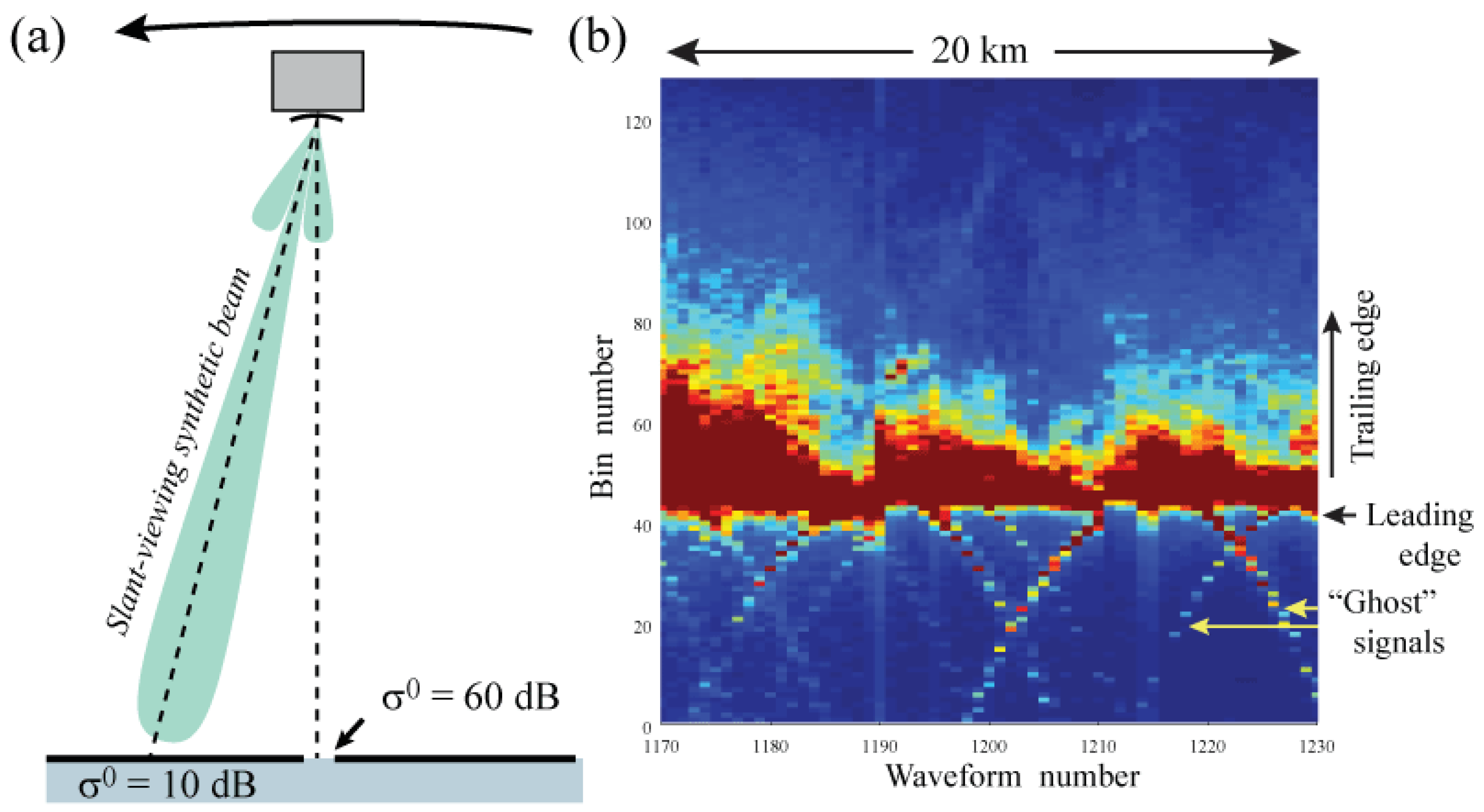
3.4.1. Snagging Effect Within Altimeter Data

In the calculation of sea surface height, there is the assumption that the range recorded on-board the satellite is that to the nearest reflecting surface, which will generally be at nadir. However, the signal from a strongly reflecting lead will dominate the return signal for many consecutive waveforms (Figure 12). The retracking algorithms tend to follow such a feature leading to large errors in the estimates of surface height, with the distance from such a “bright target” tracing out a hyperbola in the waveform data [87]. This phenomenon is referred to as “snagging” by Peacock and Laxon [33] and was given the name “off-nadir hooking” with an application to radar altimetry over rivers [88,89]. Using high-resolution MODIS imagery coincident with an Envisat track, Connor et al. [60] have shown that reflections from a lead more than 1 km off the subsatellite track can dominate the signals. Range errors related to returns from off-nadir leads have been shown to also occur for SAR altimetry data from CryoSat-2, with an underestimation of the sea surface height by 1–4 cm and strong biases in ice thickness estimation [68].
To reduce this effect and to improve the accuracy of surface height estimation, Gomez-Enri et al. [87] used a modelling approach, in which they replicated bright target features in the waveform sequence and subtracted them from the waveforms to assist the retracking process. An automatic technique was proposed by Quartly [90] to fit hyperbolic features within the waveform data. Santos da Silva et al. [88] investigated the snagging effect in ERS and Envisat data over rivers and lakes by modelling and removing the response of off-nadir reflectors. This method has been applied to correct the altimeter measurements over narrow rivers but could not describe the off-nadir distortions over large channels or lakes [88]. The correction method also required a visual inspection of range measurements close to river banks and open water and could not be implemented automatically. Maillard et al. [89] applied a pattern recognition technique to fit the sequence of surface height measurements over rivers. However, it has limited application to the measurements over sea ice, as the location and shape of leads are not known a priori.
Poisson et al. [34] improved their sea level estimates by a data-editing approach that consisted of detecting the waveforms with a strong reflection in the nadir direction and then discarding the neighbouring waveforms. This editing approach improved the retracker accuracy by discarding potentially biased range measurements around strong nadir reflection points and is illustrated in Figure 12 for the RA-2 Ku-band waveforms over Arctic leads and floes. Strong nadir reflections produced sharp spikes, which were automatically discriminated from the rest of waveforms (Figure 12b). This procedure discarded sea-level measurements around such spikes (blue dots in Figure 12c) as they were likely to produce biased results. In contrast, the output of the Giles et al. [77] retracker in Figure 12c was affected by the “snagging” effect with larger range estimates produced in the neighborhood of spikes.

3.4.2. Azimuth Ambiguity Effect Within SAR Data

The off-nadir ranging effect, as described for the LRM mode, has less impact on the SAR echoes. This is due to the along-track beam-limited resolution, but the response to across-track bright targets (such as leads) remains the same. However, it nevertheless remains present and still needs to be filtered out. However, a much more important side effect must be considered while operating in the SAR mode over sea-ice, which is known as the “side-lobe effect” or “azimuth ambiguity” effect. This effect of the SAR processing occurs while measuring low backscattering surfaces with nearby high backscattering surfaces along the track of the satellite, which is a situation typically encountered while measuring floes surrounded by leads. In this case, the weighting provided by the synthetic beam’s antenna pattern cannot fully compensate for the highly contrasting backscatter strengths. In practice, this phenomenon introduces a spurious power before the leading edge of the nadir backscatter (see Figure 13), whereas the snagging effect (in the previous subsection) introduces spurious backscatter after the leading edge, with the tails of its hyperbolae tending towards longer range. These early “ghost” peaks along the waveforms can confuse the retrackers or even corrupt the nadir peak.
Several strategies can be used to overcome this phenomenon, the first of which is the application of a Hamming filtering before the Doppler beam processing. This is the case for the ESA CryoSat-2 products but not for the Sentinel-3 products from ESA and EUMETSAT. This filter is not systematically applied on all the products because it has some minor effects on the final waveforms, including a slight reduction in the along-track resolution [91]. Two alternative approaches can be considered for products which have not filtered out the side-lobes: The first one consists simply of eliminating the waveforms that contains multiple peaks, and the second one aims to localise the peak that corresponds to the nadir and which is the one to be retracked. Only the waveforms that show clearly distinct peaks can be kept, but they may provide very useful intermittent measurements in highly fractured sea-ice areas.

3.4.3. Ensuring Consistency in Space and Time

When compiling a long-term dataset spanning multiple instruments and various retrackers, it is essential to minimise the biases between constituent parts. Although a mean bias between instruments may be determined on a global basis or via dedicated calibration sites, it is important that these offsets are also evaluated in the Arctic context. This is critical because some studies have used different retrackers for waveforms from floes, leads and open ocean, whilst others have adopted one retracker, such as TFMRA, but noted that the very different waveform shapes essentially mean that they have different retrack points [77]. Ideally, the utilisation of a unified model (see Section 3.3) should avoid any artificial change in the sea level associated with the ice edge (as the sea level is derived from open ocean waveforms on one side and predominantly from leads on the other).
Further challenges exist in the context of multi-mission datasets spanning several decades, as there have been changes in technology (LRM and SAR) and differences in processing methodology between missions (e.g., the use or not of Hamming weighting). Of particular note is that AltiKa operates at a different radar frequency to all other missions (Table 1); thus, volume scattering from snow is more significant at this frequency, leading to changes in the retrack point over ice floes [92].
A critical issue in the area of consistency is the quality and reliability of the geophysical corrections (see Section 4), since some missions enable more reliable corrections than others, e.g., due to the presence of a second radar frequency or having an on-board microwave radiometer. Finally, we note that the changes in a sea-ice cover on both seasonal and interannual scales necessitate extra care when analysing for long-term changes in sea level. The time series in Figure 14 are made from data downloaded from the Radar Altimetry Database System (RADS) using default editing (for a retrieval of the sea level from the open ocean, not from within leads) and wet tropospheric corrections from the ECMWF. Data were downloaded for four different missions in two areas: the Greenland Sea (10 W–10 E, 75–80 N) and the Beaufort Sea (150–130 W, 75–80 N). The seasonal availability of data is very different for the two regions.
Whilst the selected part of the Greenland Sea is rarely fully ice-covered, the specified region of the Beaufort Sea is ice-covered to some degree throughout most of the year but with some months (especially in recent years) returning some sea level estimates. This causes a distribution of the sea level anomaly (SLA) estimates for the latter region that is very biased towards the summer months (see Figure 14b), since data from winter and spring are flagged and discarded. In fact, most of the available data in the Beaufort Sea are obtained in late summer and early autumn, where the sea ice has reached a minimum and where there is a high risk of inaccurate range estimates due to the presence of melt ponds on the sea ice. It might be possible to recover more of the data by lowering the requirements on their quality and with different processing. Nevertheless, this seasonal variation in data quantity may affect the estimation of annual and inter-annual signals. In addition, the amplitude of the seasonal variation seems to be decreasing slightly in recent missions compared with the Envisat period. This could be due to the higher resolution of the altimeters or because of decreasing sea-ice cover.

4. Corrections and References Needed for Inferring Precise Geophysical Values

4.1. Determining Sea Level

For measuring sea level and investigating temporal changes or spatial variations associated with geostrophic currents, it is essential that no bias remains between different altimeters or between any altimeter’s processing over open ocean and over leads. Not only must the measurements be consistent but also a host of corrections need to be estimated and applied rigourously. The particular constraints within the Arctic environment are discussed below: firstly, for the atmospheric corrections (which predominantly come from models) and, secondly, for the tides and mean sea surface (which are principally based on other altimeter measurements). Section 4.1.3 gives a brief analysis of the magnitude and length scale of these corrections within the Arctic.

4.1.1. Atmospheric Corrections

In a standard open ocean altimetry processing [12,61], there are three atmospheric components that alter the propagation speed of the radio waves and one atmospheric process that affects the sea level. The three corrections are the ionospheric correction, the dry tropospheric correction (DTC) and the wet tropospheric correction (WTC). The ionospheric correction is to compensate for the effect of free electrons in the propagation path, which is a very minor effect at polar latitudes, and thus, the output from a model may be reliably used. The DTC relates to the mass of air and, thus, the surface pressure, with high-resolution meteorological reanalyses being used to calculate this correction.
Over an open ocean, WTC is normally calculated from the measurements by the on-board microwave radiometer (MWR); however, the brightness temperatures recorded by the MWR do not provide reliable estimates of atmospheric moisture over ice, and thus, the output from numerical reanalyses is again preferred (see Figure 15). Indeed, CryoSat-2, which initially had a purely cryospheric focus, does not carry an MWR. The Dynamic Atmospheric Correction (DAC) is a modelling of the sea surface response to the preceding time series of pressure and wind and is also calculated from a meteorological model [93]. The DAC comprises of both a simple “static” response to the atmospheric pressure at that time (also known as the “inverse barometer correction”) and the high-frequency “dynamic” response to the history of changes in atmospheric pressure and winds. Over the open ocean, the full DAC is normally implemented, but for the sea level under ice floes, only the simple “static” response to the pressure field is applied.

4.1.2. Tides and Mean Sea Surface

Arctic Ocean tides are generally difficult to determine as the data available are predominantly from sun-synchronous satellites. In particular, the S2 constituent, which can have a magnitude of 50 cm in the Arctic, is frozen in the orbit (i.e., the satellite always observes exactly the same phase of that tidal component), so neither it can be determined nor can sun-synchronous satellites help us disentangle the aliasing of the K1 tide and the annual sea level variation (see Table 2). Consequently, the development of new and better tide models using hydrodynamic modelling is essential for the Arctic Ocean.
The first empirical tide model of the Arctic Ocean was derived from ERS-1 data by Andersen [94]. Since then, numerous ocean tide models have been derived. Stammer et al. [95] performed a comparison for 8 state-of-the-art models with tidal constituents derived from some of the 240 Arctic tide gauges maintained by Kowalik and Proshutinsky (available via http://www.ims.uaf.edu/tide/). The agreement found is still far from as good as that noted in comparisons with tide gauges at mid to low latitudes.
To calculate the freeboard, the surface height of the ice floe has to be compared with the expectation of where the sea level would be. This is inferred by interpolating the occasional measurements within leads of the sea level relative to the mean sea surface (MSS). The MSS is, thus, the largest correction, as it ranges over more than 40 m across the Arctic Ocean, but an adequate model of the tides (including S2) is essential in order to provide an accurate MSS. The Sentinel-3 adds crucial information about the MSS north of Canada. However, the WTC correction based on MWR data must be avoided to prevent highly unrealistic values north of the Canadian Arctic Archipelago (see Figure 15).
Several MSS products exist based on different satellite altimetry input data over varying periods. Differences and properties of these products are assessed in Skourup et al. [96]. The state-of-the-art MSS fields covering the whole Arctic Ocean are the UCL13 and DTU15 MSS. (The coverage of the CNES/CLS15 MSS is incomplete, and it is therefore not generally applicable for pan-Arctic studies.) The UCL13 MSS is the one provided to the user within the ESA CryoSat-2 baseline-C data products and has been specially tuned to improve sea-ice freeboard retrieval. Outside of the Arctic, the CryoSat products revert to the CLS 2011 MSS to enable global applicability. The choice of MSS should also reflect the period of data to be analysed, as the mean will change (by definition) with time. For example, the DTU MSS surface is referenced to the 1993–2012 period and, in the Arctic, is derived from ERS-1, ERS-2, Envisat and almost six years (2010–2015) of CryoSat-2 baseline-B data. North of 88 N, this MSS is tapered towards EGM2008 GGM [97], which is a representation of the geoid.

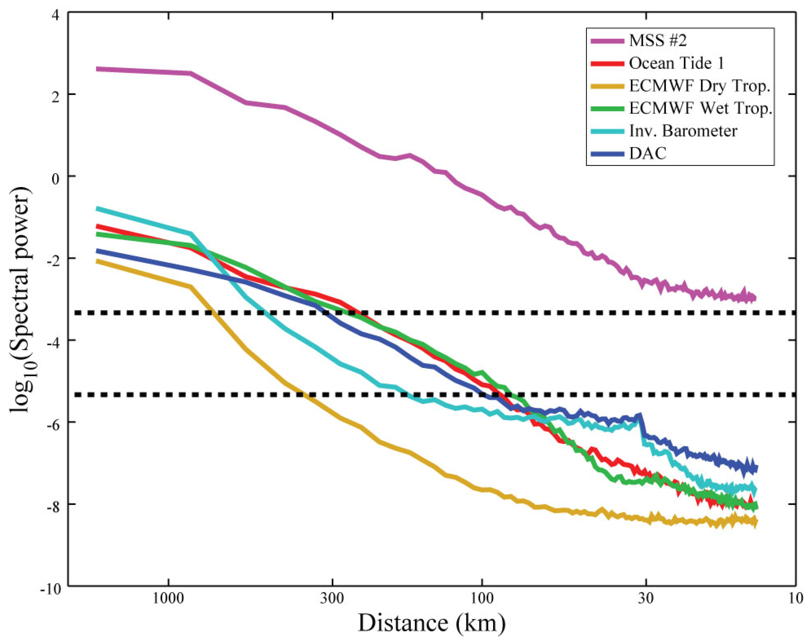
4.1.3. Amplitude and Scale Length of Corrections

Table 3 and Figure 16 show a simple analysis of the magnitude and length scales of the various corrections for Sentinel-3A. (The majority of the corrections are from models, and thus, similar values would be obtained for extracts from models along other altimeter tracks; the exceptions are WTC derived from the MWR and the ionospheric correction derived from the dual-frequency measurements.)
Table 3 shows that MSS and DTC are the largest corrections, but the latter has little spatial variation. MSS solution 1 is not appropriate for pan-Arctic studies on account of no values being supplied for 12.8% of locations, and the WTC based on MWR measurements is also invalid for many locations (as is expected when the instrument footprint is dominated by sea ice). The ionospheric correction derived from dual-frequency measurements is too noisy and frequently unavailable, as the underlying range measurements at Ku- and C-band are highly variable.
Figure 16 provides a spectral description of the pertinent corrections for Sentinel-3A. For basin scale analyses, a number of the corrections are seen to be important (i.e., contain a greater signal power than some anticipated level of white noise). The corrections appear to have a negligible impact at the mesoscale (e.g., <50 km); however, it must be recalled that these are principal corrections derived from models, and the brief analysis shown is of the corrections themselves rather than of the errors in these fields.

4.2. Determining Freeboard and Ice Thickness

4.2.1. Interpolating Sea Level Anomaly and Calculating Freeboard

Surface elevations are determined for ice floes and water in leads relative to the ellipsoid describing the approximate shape of the Earth, with the appropriate range corrections, including MSS, being subsequently applied (see Section 4.1). Next, lead elevations are interpolated to retrieve the sea level anomaly (the difference between the instantaneous sea surface height and the MSS) along the whole altimeter track. This sea level anomaly is subtracted from the sea-ice elevations to give the freeboard. Since the freeboard is a relative quantity, geophysical corrections should not affect the retrieval; however, due to spatial variations in the sea surface height between leads, interpolation errors are likely to occur. Therefore, applying geophysical range corrections (atmospheric, geophysical and MSS) is essential for minimizing such interpolation errors, which can lead to significant biases in the freeboard retrieval. The importance and impact of these range corrections on sea level anomaly and sea-ice freeboard retrievals are discussed in Skourup et al. [96] for the MSS and in Ricker et al. [43] for geophysical and atmospheric corrections. Errors in the atmospheric and oceanic corrections contribute a high frequency noise to the dynamic ocean topography (DOT) and geostrophic currents that are defined over longer time scales (i.e., weeks) and length scales (∼100 km). Errors in the DOT are calculated at orbit crossovers [33,98] or statistically at gridded level [99,100].

4.2.2. Freeboard to Thickness Conversions

In this subsection, we assume that the mean altimetric return is from the surface of the sea ice, as expected by Beaven et al. [101]; in this case, the overlying snow layer produces a path length correction due to the reduced speed of radar propagation in snow. The issue of whether the reflection is always from the ice/snow interface is addressed in Section 4.2.3. The estimation of sea-ice thickness, t i , from the altimeter-derived sea-ice freeboard is based on Archimedes Principle, assuming that the sea ice is freely floating (see Figure 17). The application of this is common to all studies using altimeter data over sea ice in the scientific literature. Variations to a certain degree do exist in the parameterization of the conversion, which requires the densities of sea ice, ρ i , sea water, ρ w and the snow load given by snow depth, t s and density ρ s as input parameters:
t i = t s · ρ s + f · ρ w ρ w ρ i
where f is the freeboard determined from the altimetry. However, aside from the uncertainty in the freeboard estimate, there is significant uncertainty in the values of the constants to be used. Whilst the density of the sea water is a well-known parameter with little variation between 1023 to 1024 kg m 3 [102], there is much less clarity about the ice density, and snow depth and density. An ice-type dependent parametrization is common for sea-ice density, which varies with the amount of brine or air bubbles entrapped in the ice layer. The main difference is the higher amount of air bubbles in multi-year ice (MYI), making its density lower than that of first-year ice (FYI). Alexandrov et al. [103] report bulk densities for level-ice of 882 ± 23 kg m 3 (MYI) and 916 ± 35.7 kg m 3 (FYI), values that are commonly used in the freeboard to thickness conversion. However, it must be noted that these values are associated with the level of sea ice only: the mean thickness of sea ice also contains a significant fraction of deformed ice where the density is likely to deviate. Other solutions, e.g., explored by Kwok and Cunningham [72] include a single bulk ice density or thickness-dependent densities.
Snow depth is not a routinely observed parameter on basin scales, a limitation that introduces a significant error component in the freeboard to thickness conversion [77,104]. The most common approach in calculating recent sea-ice thickness products [48,49,52,56,62,72] is to replace the limited observational data with a snow load climatology compiled from in situ observations in the period of 1954–91 [105]. This provides monthly fields of snow depth and density in the form of a fitted two-dimensional quadratic function and a measure of interannual variability for both depth and density. Recent airborne observations have, however, shown that the climatology overestimates snow depth in regions of FYI by as much as 50% [106,107]. Most snow climatology-based sea-ice thickness studies, therefore, apply a 50% snow depth reduction for areas of FYI. The notable exception is Kwok and Cunningham [72], who found that the agreement between the validation data and CS-2-based thickness improved when using only a 30% reduction for snow on FYI.
While the ice-type based modification of climatological snow depth may compensate for a potential trend in snow depth on sea ice, the interannual and regional variability in snow accumulation will not be mapped correctly. There have been recent efforts to infer the snow depth from the difference in observations by Ku- and Ka-band altimeters [48], but these cannot furnish values prior to the launch of AltiKa in 2013. However, Lawrence et al. [100] claim some success using a combination of Ku-band radar (Envisat) and laser (ICESat); although the operation of ICESAT was intermittent (operating for only a few months in the year), this could still contribute to a better snow-depth climatology for the 21st century. Field observations over large areas that study the relationship of freeboard and draft [108] are still required to reduce uncertainties in the freeboard to thickness conversion. In the future, the snow depth from reanalysis products may be provided as an auxiliary data source to improve the ice thickness retrieval from radar altimetry.

4.2.3. Impact of Snow on Sea-Ice Freeboard and Thickness Retrievals

The snow cover represents an additional uncertainty contributing to the remote sensing signature of sea ice. A heterogenous snow layer may affect the scattering of the radar, especially at Ku-band frequencies, such as those used by CryoSat-2. Prior to the CryoSat-2 era, it was widely assumed that the main scattering horizon at Ku-band is located at, or close to, the snow-ice interface during Arctic winter, i.e., between October and April. This assumption is based on laboratory experiments by Beaven et al. [101], who showed that, at 13.4 GHz, the radar echo originates at the snow-ice interface under dry and cold conditions with a uniform snow stratigraphy.
However, during the winter season, metamorphic processes and densification can occur, e.g., concrete snow due to wind compaction and the forming of ice lenses due to temperature gradients. Data from airborne Ku-band radar altimeters and in situ field measurements from the CryoVEx 2006 and 2008 campaigns were analyzed in Willatt et al. [109]. Their analysis reveals that, in spring 2006 at temperatures close to 0 C, only 25% of the radar returns showed the dominant scattering surface to be located close to the snow-ice interface, whereas in 2008 when the temperatures were lower, this proportion was up to 80%. They conclude that an accurate estimation of the sea-ice freeboard is only possible under dry and cold snow conditions with a known snow load and without a distinct metamorphic history. King et al. [59] found, by comparing ariborne and CryoSat-2 satellite data in a region north of Svalbard in April 2015, that even under such cold conditions the radar freeboard can be close to the snow freeboard.
Another approach to retrieving information about the scattering mechanisms at the interfaces within the snow layer and how the scattering horizons depend on the snow properties is to simulate the interaction of radar waves with snow [71,110,111]. Tonboe et al. [110] used a radiative transfer model to simulate the sea-ice effective scattering surface variability as a function of snow depth and density. They conclude that snow cover might have a variable but significant impact on the estimation of the sea-ice thickness with radar altimetry. Makynen and Hallikainen [111] have built a simulator for airborne Ku-band radar altimeter echoes over snow-covered first-year sea ice, taking into account antenna gain and pulse shape. Their results show that, for dry snow, the main scattering horizon originates at the sea-ice surface and the volume echo is negligible, but under moist snow conditions, the snow surface echo dominates.
Kwok [71] simulated the impact of the snow layer on the tracking point for determining surface elevations. He also examined airborne snow and Ku-band airborne radar data from OIB and concluded that scattering at the snow surface and within the snow layer is non-negligible and causes an alteration of the CryoSat-2 waveform tracking point that is evaluated to derive surface elevations. Similar findings have been reported by Ricker et al. [112], who compared snow and ice thickness measurements from buoys with coincident CryoSat-2 overflights. They estimated that the assumption that the main scattering horizon is represented by the snow-ice interface led to a mean ice thickness bias of 1.4 m for MYI after the strong snowfall events during 2013/2014.
Armitage and Ridout [81] derived a freeboard from CryoSat-2 Ku-band and AltiKa Ka-band radar altimeters. Using OIB airborne laser and radar measurements from spring 2013 and 2014, they evaluated the main scattering horizons for CryoSat-2 and AltiKa. For CryoSat-2 over FYI, the main scattering horizon coincides with the snow-ice interface, while over MYI, it corresponds to penetration through 82 ± 3% of the snow layer; in contrast, AltiKa echoes represent the penetration through only 46 ± 5% for both FYI and MYI.
During the formation of FYI, a brine rejection occurs both upward and downward, with the brine pool above the ice often wicked up into the subsequent snow [113]; the summer melt allows such brine to escape, such that the snow on MYI is free from brine [114]. The brine within snow affects its scattering properties [114], and in a recent study, Nandan et al. [115] investigated the effect of snow salinity on CryoSat-2 retrievals of FYI freeboard and thickness. They used in situ measurements of snow thermophysical properties on FYI in the Canadian Arctic during late winter (April/May) and found that saline snow on FYI vertically shifts the location of the main radar scattering horizon by approximately 0.07 m and, therefore, suggest introducing a snow salinity correction factor for CryoSat-2 estimates of freeboard.
To conclude, during the last decade, several studies have provided evidence that the snow layer on sea ice affects the retrieval of sea-ice freeboard and thickness from radar altimetry. However, due to differences among the existing retrieval algorithms, it is ultimately difficult to quantify this effect. Moreover, studies have shown that the impact of the snow layer varies in space and time, depending on snow properties, e.g., thickness, stratigraphy, density, salinity and temperature, and indirectly on the ice type.

5. Comparison With In Situ and Airborne Measurements

In Section 3, we showed the use of in situ, airborne and other satellite data for the validation of the waveform classification; in this section, we assess the quality of the overall physical retrievals as the results of classification, retracking and application of corrections. The first subsection deals with the oceanographic quantities, and the second deals with those relating to the sea-ice.

5.1. Sea Level and Currents

One of the first oceanographic applications of radar altimetry over the Arctic Ocean was the derivation of the marine gravity field for the permanently ice-covered regions. Laxon and McAdoo [116] analysed the mean topography of the ocean derived from the elevation measurements in leads during a 35-day cycle of ERS-1. They showed that this mean sea surface conforms to the geoid and variations of the Earth’s gravity due to density variations in the mantle (low spatial frequencies) and to sea floor topography (high frequencies). Such satellite-derived gravity fields were validated against airborne gravity surveys (i.e., Canadian Geophysical Survey) and shown to conform very well in the Beaufort Sea.
A greater precision is gained from improved altimeter measurements, and a better resolution is acquired through the denser pattern of tracks in long-repeat orbits. ERS-1 had a so-called “geodetic phase”, providing finer longitudinal sampling than in its usual 35-day repeat, but there has been a marked improvement in the Arctic marine gravity field modelling since the launch of the CryoSat-2 mission in 2010. With its 369-day repeat, it provides one cycle of geodetic mission data with 8 km global resolution each year. The higher precision of these new sea surface height observations compared with observations from ERS-1 and Geosat means that these latter data are no longer used, which has resulted in a dramatic improvement of the shorter wavelength of the gravity field (12–20 km) and s better comparison with marine gravity data [117]. The pan-Arctic altimetric gravity field DTU15 now surpasses the 2008 Arctic Gravity Field project compilation of marine gravy data from multiple sources, as can be seen from comparison with an independent gravity field from GOCE [118].
The sea surface height signal can be decomposed into two components: eustatic (change of mass of the column of water) and steric (change of ocean density). Armitage et al. [119] compared two estimates of the steric signal—integration of density profiles from ice-tethered profilers (ITPs, [120]) and altimetry minus gravity field from GRACE—and found a good correlation (R ∼ 0.86). They concluded that the Arctic SLA variability is dominated by the seasonal cycle, with the first principal component capturing 38.7% of the total SLA variance.
A mean dynamic topography (MDT), that is, the height signature consistent with the mean surface geostrophic currents, has traditionally been derived using the temporal averaging of a hydrodynamic model (such as TOPAZ or SODA). With developments in the accuracy of the MSS and geoid, the MDT can also be derived from the difference between them. The resultant MDT will consequently represent the temporal averaging period over which the corresponding MSS was derived. Farrell et al. [121] derived one of the first satellite-based MDT using ICESat; recently Andersen et al. [117] derived one called DTU15MDT (see Figure 18) taking into account GOCE and CryoSat-2 data. Its main features are consistent with an MDT derived from the TOPAZ model [122], including a signal larger than 0.3 m in the Beaufort Sea associated with the anticyclonic Beaufort Gyre and a large-scale slope (∼0.6 m/1300 km) in the topography from the Amerasian Basin to the Eurasian Basin associated with the transpolar current (see Figure 1a). Qualitatively, these results agree well with others derived from satellite altimetry [98,123] as well as from ocean models [124].
The first empirical tide model of the Arctic Ocean derived from the ERS-1 and ERS-2 altimeters [125] was validated against tide gauge measurements. Similar validations and comparisons have since been generalised to more recent models that assimilate all low inclination radar altimeters [126]. The validation of an interpolated gridded tide model against tide gauges is typically performed at the location of coastal and pelagic stations, with there being hundreds of the former but only tens of the latter. In general, an agreement between the tide models or sea surface heights derived from radar altimeters and tide gauge measurements is very good, particularly for locations away from bays and very shallow waters where strong tidal signatures are present. Armitage et al. [119] compared all Arctic tide gauge records [127] with more than 72 months of data for the 2003–2014 period, covering measurements from Envisat and CryoSat-2, and confirmed this good agreement for tide gauges in the Canadian Arctic, Barents Sea and Svalbard (R ∼ 0.8–0.9), while correlations for stations in the Kara, Laptev and East Siberian Seas were found to be lower (R ∼ 0.5–0.7) due to the larger impact of seasonal runoff and to the proximity to river estuaries. Recently, Armitage et al. [128] produced a 12-year time series of geostrophic currents in the Arctic and performed the first direct evaluation against in situ measurement by three acoustic Doppler current profilers (ADCPs) in the Beaufort Sea, showing a significant correlation in speed for two out of three moorings and a significant correlation in the bearing for one of them. Some of the differences are explained by the difference in footprint and timescale over which the data are collected for both techniques.

5.2. Freeboard and Sea-Ice Thickness

There are several different methods to evaluate the satellite-derived sea-ice freeboard and thickness. Through the years of satellite altimetry, in situ observations, airborne campaigns, submarines, and drifting and moored buoys have all been invaluable in measuring the sea-ice and snow properties. However, as it is difficult and expensive to operate in the harsh environment with cold temperatures and darkness during the Arctic winter, such observations are still sparsely distributed in space and time (see Figure 19).
The various evaluation data sets have their own pros and cons with respect to spatial and temporal resolution. Airborne and submarine surveys cover larger areas and usually represent short temporal scales (days or months), whereas the moored and drifting buoys represent point measurements over longer time scales and provide information about seasonal variations.

5.2.1. Freeboard

There are two reasonably extensive datasets for a direct satellite sea-ice freeboard evaluation. One is from NASA’s Operation IceBridge, with the sea-ice freeboard given by the total freeboard (snow + sea ice) measured by a laser altimeter minus the snow depth measured by the snow radar. The other is from the airborne campaigns carried out as part of ESA’s CryoSat Validation Experiment (CryoVEx), where ASIRAS (an airborne version of the CryoSat-2 SIRAL altimeter) provides coincident Ku-band radar freeboard data. More recent campaigns (2016 and 2017) have included an airborne Ka-band radar altimeter (KAREN) to evaluate SARAL/AltiKa and to exploit the potential of a dual-frequency concept for future satellite missions. The processing of the KAREN data is still ongoing, so results can not be included here. The measurements obtained by the OIB snow radar also provide a valuable validation of snow depth.
The airborne OIB and CryoVEx data are primarily used to evaluate the satellite radar freeboard, to investigate penetration depths of both Ku- and Ka-band radars and the potential for snow-depth retrieval [60,81,92,100,129] and to examine the sensitivity to the choice of using different retrackers [56,62]. These studies consistently conclude that the predominant signal from Ku-band satellite radars such as CryoSat-2 and Envisat corresponds to the reflections from close to the snow-ice boundary. Other studies of CryoSat-2 [59,112] used Ice Mass Balance (IMB) buoys and a combination of airborne and in situ measurements of sea-ice and snow properties to show that the influence of snow cover on Ku-band penetration is not negligible in specific regions and/or snow conditions (see Section 4.2.3). A recent paper [130] compared the output of three different retrackers applied to CryoSat-2 data with the freeboard measurements recorded by ATM and noted that their threshold retracker was the best for MYI, whereas a waveform-fitting approach gave superior results for FYI.
A wider range of conclusions was found for the Ka-band radar altimeter (SARAL/AltiKa). Guerreiro et al. [92] concluded that AltiKa’s signals corresponded to a reflection at the air-snow surface, Armitage and Ridout [81] concluded that they were almost half-way between the air-snow and snow-ice surface, and Maheshwari et al. [129] concluded that they were at the snow-ice surface. Lawrence et al. [100] found a surface-dependent bias of the AltiKa radar freeboard against airborne snow freeboard. The use of different retrackers as well as the consideration of the impact of sea-ice roughness could explain some of these inconsistencies.

5.2.2. Sea-Ice Thickness (SIT)

In the literature the most commonly used observations to evaluate satellite-derived SIT are values derived from the NASA operation IceBridge (OIB), total (sea ice + snow) thickness by airborne electromagnetic (AEM) sensors and sea-ice draft. The latter is measured by upward-looking sonars (ULS) either from submarine cruises or moored buoys (for example, during the Beaufort Gyre Experiment; BGEP). A more detailed description of these data sets is found in Lindsay and Schweiger [131] and Kwok and Cunningham [72]. As none of the abovementioned observations measure the SIT directly, the satellite-derived estimates need to be changed into either draft or total thickness before a comparison, with a priori assumptions of snow depth and/or densities of snow and sea ice. In addition, SIT obtained by OIB are derived by the measured total freeboard and snow depth according to Equation (2). Thus, in order to compare the values from satellite altimetry with the in situ observations, it is important to have consistent assumptions about the snow depth and the densities of sea ice, snow and water.
Despite these challenges and the many assumptions in the processing chain, recent studies (e.g., References [49,52,72]) find relatively good correlations (0.5–0.9) with mean differences 0 . 21 to 0.12 m between the CryoSat-2-derived SIT products and the evaluation data in the central Arctic winter (October–March). Prior studies comparing ERS-1 and ERS-2 with draft from submarine cruises [32] found an almost one-to-one agreement. These results are within the expected uncertainties of measurements, and no systematic biases were found. Often the correlation between OIB and CryoSat-2 SIT estimates are found to be lower than with submarine, moored buoys and AEM observations. The cause of this is still unclear and subject to further investigation [52,72].

5.2.3. Validation of Algorithms

Last but not least, the total thickness of sea-ice + snow by AEM sensors and the sea-ice draft from moorings have also been used to evaluate and improve various steps in the processing chain, such as the Envisat freeboard retrieval by including information about the surface roughness [48]. Submarine, airborne and buoy data have also been used in sensitivity studies to investigate the parameters (snow depth and densities of sea ice) used in the freeboard to sea-ice thickness conversion (see Equation (2)). No consistent results were found, as Kern et al. [104] found it important to use different densities for FYI and MYI, whereas Kwok and Cunningham [72] found the best correlation using only one density representative of FYI. Kwok and Cunningham [72] also found the snow depth to be best represented by taking 70% of the Warren snow depth [105] over FYI as opposed to 50% used in Laxon et al. [52]).

6. Future Prospects: Expectations and Hopes

This appears to be a very propitious time for Arctic studies, with many decades of data available enabling further honing of algorithms and with the prospect of new satellite missions, in situ data and new initiatives to utilise multiple datasets synergetically. We consider, below, some of the areas in which further advances may be anticipated.

6.1. Improvements in Processing

Although the launch of CryoSat-2 in 2010 heralded a new era in Arctic altimetry, with its high inclination orbit and finer resolution through SAR processing, there still remains much to be done with the preceding two decades of LRM altimetry. Recent advances in data storage and computer processing power mean that many people now have the potential to process the entire ERS-1, ERS-2 and Envisat waveform datasets rather than always using the products derived by the space agencies. This has been greatly assisted by ESA’s REAPER project [132], which has made the data from early missions more readily accessible, coupled with improved orbits and corrections.
A further understanding of radar reflections from snow upon sea-ice is required, as the scattering horizon varies according to the temperature and salinity of the snow (see Section 4.2.3). This knowledge, especially for differences in snow properties on FYI and MYI, could be gained through both modelling and in situ studies in the Arctic (see Section 6.5) and would also be complemented by improved datasets on the depth of snow. Although there have not been many papers providing a quantitative assessment of the classification strategies, there have been a number of new ideas for methodologies, especially for SAR waveforms. However, these still need to be thoroughly evaluated, especially for their ability to separate melt ponds from leads, as the former make it difficult to recover the sea level within the ice floes during summer.
A number of new processing strategies have been developed [34,83] which have yet to be applied to the full set of data on the 35-day ERS/Envisat orbit. Further improvements in retracking and quality control may be expected. Firstly, this will encompass improved statistical approaches to select the different echo types, but potentially, there may also be retracking algorithms that utilise the extra information in waveforms adjacent to a lead rather than solely retracking the single return directly over it. Such an approach, gathering information from across the hyperbolic trajectory (see Figure 12), could build on previous ideas for detecting individual bright targets [87,133,134].

6.2. New Missions with New Capabilities

Table 1 catalogued all the radar altimetry missions covering the Arctic beyond 72 N, including Sentinel-3B launched in April 2018. The recent Sentinel-3 missions not only offer the prospect of many decades of further coverage through subsequent launches but also offer the potential to improve the historical record. This is because, early in their combined tandem mission observing the same ground track 30 seconds apart, one operated as a SAR altimeter with the other in LRM mode. This enables a much closer comparison of waveform classification and retracking in these two different modes. The understanding gained about their differential response to, say, small leads or melt ponds, can be used to develop a more consistent processing scheme to deliver the homogeneous datasets on the Arctic sea level and freeboard that are required for climate studies.
The Envisat radar altimeter RA-2 worked not only at the Ku-band but also at the S-band, which was exploited for ice studies over Antarctica and Greenland [135,136]. However, this was only rarely used for ice classification over the Arctic [137], as the information from the passive MWR was more useful in that study than the S-band radar measurements. The potential advantages of dual-frequency altimetry may be better realised with the Sentinel-3 spacecraft, since their measurements (at the C-band) have the same width sampling bins as at the Ku-band (which was not the case for Envisat) and, thus, a better recording of the waveforms at the secondary frequency. Figure 20 shows the mean difference between the backscatter strengths ( σ K u 0 and σ C 0 ) for three different months over the winter 2016/17. The chosen scaling for the Sentinel-3 σ 0 values makes the mean values over the ocean similar (although there is some variation with wind conditions). The series of three plots shows the expanding area of sea ice (confirmed by the 50% SIC contour in pink), with the recently-formed ice having a σ K u 0 σ C 0 signature of approx. 1.5 to 2.5 dB, but the regions where ice has been present for several months shows negative values. This possibly points to some change in the sea-ice properties over the first few months, but it does not provide a distinction between FYI and MYI. Work to support the use of these auxiliary measurements needs to be encouraged.
There are also plans for successor missions for both AltiKa and CryoSat-2. In particular, CryoSat-2 has been operating for almost 9 years, and there is a compelling case for another mission to observe the Arctic poleward of 81.5 N, as this regions contains most of the MYI. Future missions not only will help ensure the long-term recording of Arctic sea level and ice freeboard but also could improve the snow depth climatology through the joint exploitation of the Ku-band and Ka-band data [48].
This review paper has focused on radar altimetry only. However, NASA’s ICESat mission [138] carried a laser altimeter that has been operated between February 2003 and October 2009, with the capability to retrieve freeboard [139]. However, in contrast to radar altimetry, laser altimetry is affected by clouds, and ICESat measurements were restricted to two periods per winter season (October/November and February/March). The combination of laser and radar altimtery is challenging because of the very different footprint sizes, effect of clouds on laser measurements and different characteristics of the penetration into the snowpack on top of the ice. However, the launch of ICESat-2 (15 September 2018) should prompt renewed effort to combine radar and laser range measurements. The Advanced Topographic Laser Altimeter System (ATLAS) onboard ICESat-2 uses a multi-beam approach with 6 laser beams, arranged in 3 pairs pointed on the ground at intervals of 3.3 km across a track [140]. Coincident measurements of ICESat-2 and CryoSat-2 also have the potential capability to estimate snow depth.

6.3. Realizing the Potential of SAR Interferometry (SARin)

CryoSat-2 has pioneered two advances in altimetry. As well as being the first spaceborne system to use SAR altimetry, it has a second antenna 1.2 m across track from the one that both transmits and receives signals. This gives it an interferometric capability, as the phase of the signals received by the two antennas can be compared to determine the off-nadir location of the signal [141]. The original purpose was to map the exact location of the return signal in areas with a highly varying topography such as glaciers, smaller ice caps and margins of ice sheets [26] (see Figure 21), but it has also been shown to improve the retrieval of sea surface heights in coastal [142,143] and sea-ice-covered regions [68], thus reducing the uncertainty of sea-ice freeboard heights [144].
As described in Section 3.4.1 snagging leads to underestimates in the sea surface height due to locking on bright off-nadir targets. This highly affects classical altimetry observations due to the large footprints and even affects CryoSat-2 in the SAR mode by recording bright targets that are up to 13 km in the across-track direction [142,145] which is outside the nominal across-track footprint size. Such snagging events are normally circumvented by suitable retracking and discarding waveforms including reflections from off-nadir leads.
Usually, the sea surface height and sea-ice freeboard in SARIn areas are processed using a SAR-like approach [49,146] with degraded noise levels compared with the real SAR acquisition due to the lower burst repetition frequency of the SARIn mode [26]. By using the phase information from the SARIn mode to range correct off-nadir leads, the accuracy and precision of the estimated sea surface height is improved by increasing the number of valid waveforms despite the degraded noise level [68]. The inclusion of the increased number of retrieved sea surface height estimates (with only approx. 35% of the discarded waveforms of the SAR-like case) results in a reduction of the total random freeboard uncertainty of 40% [144].
The SARIn capabilities are currently a unique feature of the CryoSat-2 altimeter mission and are restricted to specified areas of complex topography. However, the launch of the NASA/CNES Surface Water and Ocean Topography (SWOT) mission in 2021 will provide the Ka-band SARIn altimetry globally between 78 S and 78 N. To support further investigations of the advantages and limitations of SARIn altimetry, most recent ESA CryoVEx campaigns in 2017/2018 have collected airborne Ka-band altimetry data in SARIn mode in the Arctic and Antarctic (see also Section 5.2) along selected CryoSat-2, Sentinel-3A and AltiKa ground tracks [147]. This was epitomised by a coordinated sea-ice flight involving, for the first time, four aircrafts carrying a suite of instruments to monitor the snow and sea ice along a CryoSat-2 ground track.

6.4. Utilising Data Fusion Techniques

Due to the sensor and orbit characteristics, satellite retrievals of SIT differ in spatial and temporal resolution as well as in the sensitivity to certain sea-ice types and thickness ranges. The aim of satellite data fusion is to take advantage of the complementarity of retrievals derived from different satellite sensors.
One of the major objectives of the CryoSat-2 radar altimeter mission is the retrieval of Arctic SIT, with it being designed to observe thick first-year and perennial sea ice, but it has a larger relative uncertainty for thin seasonal sea ice. CryoSat-2 uncertainties contain contributions that are associated with speckle noise, sea surface height estimation, snow depth, and densities of ice and snow [56].
On the other hand, the 1.4 GHz (L-band) radiometer on the SMOS (Soil Moisture and Ocean Salinity) satellite has been used successfully to retrieve the thickness of thin ice in the marginal ice zone and during the freeze-up [148]. The method is based on analyzing the surface brightness temperatures using a thickness-dependent emission model, and the overall uncertainty contains contributions from the errors in measured brightness temperatures, the uncertainty in sea-ice salinity and temperature, as well as the assumptions for radiation and thermodynamic models [149].
Figure 22 shows the relative uncertainties (as calculated in Ricker et al. [70]) for CryoSat-2 and SMOS monthly means for the winter season 2013/2014. While the SMOS uncertainties are low over thin ice (<1 m), SMOS’s sensitivity for thicker ice (>1 m) is limited and thicknesses above 1.5 m are not retrieved. In contrast, the absolute uncertainty of CryoSat-2 estimates over thick ice is the same or less than that over thin ice, so the relative uncertainty drops with increasing SIT.
Ricker et al. [70] developed a method of completing and improving Arctic SIT information by merging CryoSat-2 and SMOS retrievals based on an optimal interpolation scheme. The merged product overcomes several issues associated with single-mission retrievals and provides a more accurate and comprehensive view on the state of Arctic sea-ice thickness. This approach can be adopted for recently launched altimeter missions such as Sentinel-3A and Sentinel-3B. Their orbital inclination (see Table 1) results in a larger pole hole (region of no altimeter observations), but on the other hand, the density of Sentinel-3 orbits at 81.4 N is much higher than for CryoSat-2, which leads to a synergetic effect when both missions are combined. However, the continued operation of an altimeter in a CryoSat-like orbit is essential for monitoring SIT north of the turning latitude of the Sentinel-3 missions.

6.5. Enhanced in Situ Observations

In the derivation of freeboard from altimetry data, a major source of error is the uncertainties in the various physical constants used in the calculation (see Equation (2)). The snow depth climatology is from a study by Warren et al. [105], which is based on in situ observations obtained during 1954–1991 and is no longer representative of the current snow depth conditions [57]. For the sea-ice density, most studies use the measurements provided by Alexandrov et al. [103], which are not only outdated (1928–1993) but also restricted to the coastal Siberian regions and are, therefore, not representative of the entire Arctic basin. In this context, new measurements of sea-ice density and snow depth should be obtained at the basin scale in order to update the current parametrizations used to convert the freeboard height to ice thickness.
A major advance is likely to come from the MOSAIC programme [150], in which the RV PolarStern will act as the central observation site for an international 12-month multidisciplinary study that will encompass measuring the snow depth and morphology, as well as the ice draft, on a variety of scales. In particular, there will be surveys on at least a weekly basis at a number of sites spanning different sea-ice conditions, which will include the development of melt ponds during the thaw cycle. Such a large programme will not only furnish a better parameterization of the factors affecting these constants but also create a useful database of validation data. However, even such a campaign, which will be lodged within FYI, cannot fully address the diversity of conditions across the whole Arctic, and so, contributions from other drifting stations, icebreaker missions and dedicated cal/val exercises (e.g., associated with ICESat-2) will still be essential.

7. Conclusions

This paper has provided a review of the technical aspects of radar altimetry over the Arctic for both sea level and sea-ice studies and complements the scientific review provided by Johannessen and Andersen [1]. It has shown how the surface type affects the shape and strength of the return waveforms, both for LRM and SAR (delay-Doppler) altimeters. It has covered the challenges of robustly classifying the waveforms (and also of assessing such a classification) and then developing retracking approaches for deriving the height of the reflecting surface, especially with spurious extra signals due to off-nadir bright targets.
A persistent issue is that of reliably classifying data according to surface type. Whilst there are a plurality of solutions (with many just having a visual validation for a selected scene), there have been few papers that compared several methods quantitatively against reliable independent datasets. Even the statistical or machine-learning approaches typically rely on some subjective operator classifications as their reference. Effort is required to collate all the available ground truth data (whether in situ or from airborne or spaceborne sensors) that coincide with satellite altimetry. Open access to such an extensive database, plus protocols for systematic validation, would allow new approaches to be more reliably benchmarked. An important aspect of this is the need to also improve the quality of the corrections, especially the density of ice and the depth and density of the overlying snow and its microstructure, some of which will be addressed by a major international in situ campaign, MOSAIC [150]. For the geophysical products (principally, sea level and sea ice thickness), further developments in the interpolation and mapping may be required that better accommodate the short-correlation lengths and the non-synoptic nature of each month’s observations.
Whilst we have the benefit of 25+ years of Arctic altimetry data, the accurate estimation of potential climate-related change is still very challenging because of the need to understand the differences between all the altimeters. ESA’s long-term vision for 15 years of Sentinel-3 altimetry provides some confidence that the majority of the Arctic will continue to be monitored, but there is a potential gap in the coverage north of 81.5 N if CryoSat-2 ceases operation. The need for in situ measurements remains strong, not only for the purpose of satellite validation but also to provide a better understanding of the factors (snow depth, melt ponds and refreezing of leads) that affect the altimeter’s waveforms.

Author Contributions

This review article was led and coordinated by G.Q. with contributions of text and figures from E.R., M.P., O.B.A., S.D., S.F., A.G., S.H., A.A.K., F.L.M., R.R., H.S. and M.T. All authors contributed to the internal review and commented on revisions.

Funding

This review work principally made use of the authors’ existing knowledge and expertise. G.Q. is grateful for the financial support of the European Space Agency through the Sentinel-3 Mission Performance Centre (Contract no. 4000111836/14/I-LG) to permit time for collating and merging these contributions.

Acknowledgments

The authors were originally supported by the European Space Agency for work towards their Climate Change Initiative programme (Sea Level CCI and Sea Ice CCI). The opportunity for cross-disciplinary discussion was assisted by two meetings funded by the International Space Science Institute. We acknowledge the contributions to those discussions made by Pierre Thibaut, Jean-Christophe Poisson and Kevin Guerreiro and are sad that they were unable to contribute to this paper. G.Q. thanks Francesco Nencioli for the help with the LaTeX formatting and Dawn Ashby for advice with Illustrator. The data on the climatological sea-ice extent were provided by the NASA National Snow and Ice Data Center Distributed Active Archive Center (NSIDC DAAC).

Conflicts of Interest

The authors declare no conflict of interest. The European Space Agency, who funded the CCI work, retained an active interest in the development of the work through their Technical Officers, Jerome Benveniste and Pascal Lecomte, but they had no role in the writing of this manuscript.

Abbreviations

The following abbreviations are used in this manuscript:
ADCPAcoustic Doppler Current Profilermssmean square slope
AEMAirborne ElectroMagnetic sensorMSSMean Sea Surface
AGCAutomatic Gain ControlMWRMicrowave Radiometer
ALESAdaptive Leading Edge Sub-waveformMYIMulti-Year Ice
ALOSAdvanced Land Observation SatelliteNNNeural Net
ATMAirborne Topographic MapperNSIDCNational Snow and Ice Data Center
BGEPBeaufort Gyre Exploration ProjectOCOGOffset Centre-Of-Gravity
BHBrown-HayneOIBOperation IceBridge
CCIClimate Change InitiativeOLCIOcean and Land Colour Instrument
CPOMCentre for Polar Observation and ModellingPLRMPseudo Low-Rate Measurement
CryoVExCryosat Validation ExperimentPPPulse Peakiness
DACDynamic Atmosphere CorrectionPTRPoint Target Response
DDADelay-Doppler AltimeterRARadar Altimeter
DOTDynamic Ocean TopographyRIPRange-Integrated Power
DTCDry Tropospheric CorrectionSAMOSASAR Altimetry MOde Studies and Applications
ERSEuropean Remote-sensing SatelliteSARSynthetic Aperture Radar
EnvisatEnvironmental SatelliteSARinSAR interferometry
ESAEuropean Space AgencyS.D.Standard Deviation
FFTFast Fourier TransformSICSea-Ice Concentration
FYIFirst Year IceSITSea-Ice Thickness
GDRGeophysical Data RecordSKStack Kurtosis
GOCEGravity field and steady-state OceanSLASea Level Anomaly
Circulation ExplorerSMMRScanning Multichannel Microwave Radiometer
GRACEGravity Recovery and Climate ExperimentSMOSSoil Moisture and Ocean Salinity
ICESatIce, Cloud, and land Elevation SatelliteSPStack Peakiness
IMBIce Mass BalanceSRALSentinel-3 Radar Altimeter
LEWLeading Edge WidthSSStack Skewness
LRMLow Rate MeasurementSSDStack Standard Deviation
MDTMean Dynamic TopographySSM/ISpecial Sensor Microwave/Imager
MERISMedium Resolution Imaging SpectrometerTESTrailing Edge Slope
MODISModerate Resolution ImagingTFMRAThreshold First Maximum Retracker Algorithm
SpectroradiometerULSUpward-Looking Sonar
MPMaximal PowerWTCWet Tropospheric Correction

References

  1. Johannessen, J.; Andersen, O. The high latitudes and polar ocean. In Satellite Altimetry over Oceans and Land Surfaces; Stammer, D., Cazenave, A., Eds.; CRC Press: Boca Raton, FL, USA, 2017; Chapter 8; pp. 271–294. [Google Scholar]
  2. Gloersen, P.; Campbell, W.J.; Cavalieri, D.J.; Comiso, J.C.; Parkinson, C.L.; Zwally, H.J. Satellite passive microwave observations and analysis of Arctic and Antarctic sea ice, 1978–1987. Ann. Glaciol. 1993, 17, 149–143. [Google Scholar] [CrossRef]
  3. Perrette, M.; Yool, A.; Quartly, G.D.; Popova, E.E. Near-ubiquity of ice-edge blooms in the Arctic. Biogeoscience 2011, 8, 515–524. [Google Scholar] [CrossRef] [Green Version]
  4. World Meteorological Organization (WMO). WMO Sea Ice Nomenclature Technical Report; World Meteorological Organization: Geneva, Switzerland, 2014. [Google Scholar]
  5. AMAP. Snow, Water, Ice and Permafrost in the Arctic (SWIPA) 2017; Technical Report; Arctic Monitoring and Assessment Programme AMAP: Oslo, Norway, 2017; ISBN 978-82-7971-101-8. [Google Scholar]
  6. Lind, S.; Ingvaldsen, R.B.; Furevik, T. Arctic warming hotspot in the northern Barents Sea linked to declining sea-ice import. Nat. Clim. Chang. 2018, 8, 634–639. [Google Scholar] [CrossRef]
  7. Barton, B.I.; Lenn, Y.D.; Lique, C. Observed Atlantification of the Barents Sea causes the Polar Front to limit the expansion of winter sea ice. J. Phys. Oceanogr. 2018, 48, 1849–1866. [Google Scholar] [CrossRef]
  8. Stroeve, J.; Notz, D. Changing state of Arctic sea ice across all seasons. Environ. Res. Lett. 2018, 13, 103001. [Google Scholar] [CrossRef]
  9. Screen, J.A.; Williamson, D. Ice-free Arctic at 1.5 C? Nat. Clim. Chang. 2017, 7, 230–231. [Google Scholar] [CrossRef]
  10. Jahn, A. Reduced probability of ice-free summers for 1.5 C compared to 2 C warming. Nat. Clim. Chang. 2018, 8, 409–413. [Google Scholar] [CrossRef]
  11. Rinke, A.; Maslowski, W.; Dethloff, K.; Clement, J. Influence of sea ice on the atmosphere: A study with an Arctic atmospheric regional climate model. J. Geophys. Res. Atmos. 2006, 111, D16. [Google Scholar] [CrossRef]
  12. Quartly, G.; Legeais, J.F.; Ablain, M.; Zawadzki, L.; Fernandes, M.; Rudenko, S.; Carrère, L.; García, P.N.; Cipollini, P.; Andersen, O.; et al. A new phase in the production of quality-controlled sea level data. Earth Syst. Sci. Data 2017, 9, 557–572. [Google Scholar] [CrossRef] [Green Version]
  13. Legeais, J.F.; Ablain, M.; Zawadzki, L.; Zuo, H.; Johannessen, J.A.; Scharffenberg, M.G.; Fenoglio-Marc, L.; Fernandes, M.J.; Andersen, O.B.; Rudenko, S.; et al. An improved and homogeneous altimeter sea level record from the ESA Climate Change Initiative. Earth Syst. Sci. Data 2018, 10, 281–301. [Google Scholar] [CrossRef] [Green Version]
  14. Paul, S.; Hendricks, S.; Ricker, R.; Kern, S.; Rinne, E. Empirical parametrization of Envisat freeboard retrieval of Arctic and Antarctic sea ice based on CryoSat-2: progress in the ESA Climate Change Initiative. Cryosphere 2018, 12, 2437–2460. [Google Scholar] [CrossRef]
  15. GCOS. Systematic Observation Requirements for Satellite-Based Data Products for Climate. 2011 Update; Technical Report; GCOS: 2011. Available online: http://cci.esa.int/sites/default/files/gcos-154.pdf (accessed on 10 April 2019).
  16. Proshutinsky, A.; Ashik, I.M.; Dvorkin, E.N.; Häkkinen, S.; Krishfield, R.A.; Peltier, W.R. Secular sea level change in the Russian sector of the Arctic Ocean. J. Geophys. Res. Oceans 2004, 109, C3. [Google Scholar] [CrossRef]
  17. Proshutinsky, A.; Dukhovskoy, D.; Timmermans, M.L.; Krishfield, R.; Bamber, J.L. Arctic circulation regimes. Philos. Trans. R. Soc. Lond. A Math. Phys. Eng. Sci. 2015, 373. [Google Scholar] [CrossRef]
  18. Kwok, R.; Rothrock, D.A. Decline in Arctic sea ice thickness from submarine and ICESat records: 1958–2008. Geophys. Res. Lett. 2009, 36. [Google Scholar] [CrossRef]
  19. Cavalieri, D.; Parkinson, C.; Gloersen, P.; Zwally, H. Sea Ice Concentrations from Nimbus-7 SMMR and DMSP SSM/I-SSMIS Passive Microwave Data, Version 1. Dataset 0051. Available online: https://nsidc.org/data/NSIDC-0051/versions/1 (accessed on 10 April 2019).
  20. Chelton, D.B.; deSzoeke, R.A.; Schlax, M.G.; El Naggar, K.; Siwertz, N. Geographical variability of the first baroclinic Rossby radius of deformation. J. Phys. Oceanogr. 1998, 28, 433–460. [Google Scholar] [CrossRef]
  21. ISO. ISO19906:2010 Petroleum and Natural Gas Industries–Arctic Offshore Structures; Technical Report; ISO: Geneva, Switzerland, 2010. [Google Scholar]
  22. IMO. International Maritime Organization Polar Code; Technical Report; IMO: London, UK, 2017. [Google Scholar]
  23. Chelton, D.B.; Walsh, E.J.; MacArthur, J.L. Pulse compression and sea level tracking in satellite altimetry. J. Atmos. Ocean. Technol. 1989, 6, 407–438. [Google Scholar] [CrossRef]
  24. Steunou, N.; Desjonquères, J.D.; Picot, N.; Sengenes, P.; Noubel, J.; Poisson, J.C. AltiKa altimeter: Instrument description and in flight performance. Mar. Geodesy 2015, 38, 22–42. [Google Scholar] [CrossRef]
  25. Raney, R.K. The delay/Doppler radar altimeter. IEEE Trans. Geosci. Remote Sens. 1998, 36, 1578–1588. [Google Scholar] [CrossRef]
  26. Wingham, D.; Francis, C.; Baker, S.; Bouzinac, C.; Brockley, D.; Cullen, R.; de Chateau-Thierry, P.; Laxon, S.; Mallow, U.; Mavrocordatos, C.; et al. CryoSat: A mission to determine the fluctuations in Earth’s land and marine ice fields. Adv. Space Res. 2006, 37, 841–871. [Google Scholar] [CrossRef]
  27. Brown, G. The average impulse response of a rough surface and its applications. IEEE Trans. Antennas Propag. 1977, 25, 67–74. [Google Scholar] [CrossRef]
  28. Hayne, G. Radar altimeter mean return waveforms from near-normal-incidence ocean surface scattering. IEEE Trans. Antennas Propag. 1980, 28, 687–692. [Google Scholar] [CrossRef] [Green Version]
  29. Amarouche, L.; Thibaut, P.; Zanife, O.; Dumont, J.P.; Vincent, P.; Steunou, N. Improving the Jason-1 ground retracking to better account for attitude effects. Mar. Geodesy 2004, 27, 171–197. [Google Scholar] [CrossRef]
  30. Laxon, S.W. Sea ice extent mapping using the ERS-1 radar altimeter. Adv. Remote Sens. 1994, 3, 112–116. [Google Scholar]
  31. Zakharova, E.A.; Fleury, S.; Guerreiro, K.; Willmes, S.; Rémy, F.; Kouraev, A.V.; Heinemann, G. Sea ice leads detection using SARAL/AltiKa altimeter. Mar. Geodesy 2015, 38, 522–533. [Google Scholar] [CrossRef]
  32. Laxon, S.W.; Peacock, N.; Smith, D. High interannual variability of sea ice thickness in the Arctic region. Nature 2003, 425, 947–950. [Google Scholar] [CrossRef]
  33. Peacock, N.R.; Laxon, S.W. Sea surface height determination in the Arctic Ocean from ERS altimetry. J. Geophys. Res. Oceans 2004, 109. [Google Scholar] [CrossRef] [Green Version]
  34. Poisson, J.C.; Quartly, G.D.; Kurekin, A.A.; Thibaut, P.; Hoang, D.; Nencioli, F. Development of an ENVISAT altimetry processor providing sea level continuity between open ocean and Arctic leads. IEEE Trans. Geosci. Remote Sens. 2018, 56, 5299–5319. [Google Scholar] [CrossRef]
  35. Lee, S.; Im, J.; Kim, J.; Kim, M.; Shin, M.; Kim, H.C.; Quackenbush, L.J. Arctic sea ice thickness estimation from CryoSat-2 satellite data using machine learning-based lead detection. Remote Sens. 2016, 8, 698. [Google Scholar] [CrossRef]
  36. Zygmuntowska, M.; Khvorostovsky, K.; Helm, V.; Sandven, S. Waveform classification of airborne synthetic aperture radar altimeter over Arctic sea ice. Cryosphere 2013, 7, 1315–1324. [Google Scholar] [CrossRef] [Green Version]
  37. Müller, F.L.; Dettmering, D.; Bosch, W.; Seitz, F. Monitoring the Arctic seas: How satellite altimetry can be used to detect open water in sea-ice regions. Remote Sens. 2017, 9, 551. [Google Scholar] [CrossRef]
  38. Gommenginger, C.; Thibaut, P.; Fenoglio-Marc, L.; Quartly, G.; Deng, X.; Gómez-Enri, J.; Challenor, P.; Gao, Y. Retracking Altimeter Waveforms Near the Coasts. In Coastal Altimetry; Vignudelli, S., Kostianoy, A.G., Cipollini, P., Benveniste, J., Eds.; Springer: Berlin/Heidelberg, Germany, 2011; pp. 61–101. [Google Scholar]
  39. Dettmering, D.; Wynne, A.; Müller, F.L.; Passaro, M.; Seitz, F. Lead detection in polar oceans—A comparison of different classification methods for Cryosat-2 SAR data. Remote Sens. 2018, 10, 1190. [Google Scholar] [CrossRef]
  40. Longépé, N.; Thibaut, P.; Vadaine, R.; Poisson, J.; Guillot, A.; Boy, F.; Picot, N.; Borde, F. Comparative evaluation of sea ice lead detection based on SAR imagery and altimeter data. IEEE Trans. Geosci. Remote Sens. 2019. accepted. [Google Scholar]
  41. Wernecke, A.; Kaleschke, L. Lead detection in Arctic sea ice from CryoSat-2: Quality assessment, lead area fraction and width distribution. Cryosphere 2015, 9, 1955–1968. [Google Scholar] [CrossRef]
  42. Passaro, M.; Müller, F.L.; Dettmering, D. Lead detection using Cryosat-2 delay-doppler processing and Sentinel-1 SAR images. Adv. Space Res. 2017, 62, 1610–1625. [Google Scholar] [CrossRef]
  43. Ricker, R.; Hendricks, S.; Beckers, J.F. The impact of geophysical corrections on sea-ice freeboard retrieved from satellite altimetry. Remote Sens. 2016, 8, 317. [Google Scholar] [CrossRef]
  44. Shen, X.; Zhang, J.; Zhang, X.; Meng, J.; Ke, C. Sea ice classification using Cryosat-2 altimeter data by optimal classifier-feature assembly. IEEE Geosci. Remote Sens. Lett. 2017, 14, 1948–1952. [Google Scholar] [CrossRef]
  45. Lindsay, R.W.; Rothrock, D.A. Arctic sea ice leads from advanced very high resolution radiometer images. J. Geophys. Res. Oceans 1995, 100, 4533–4544. [Google Scholar] [CrossRef]
  46. Willmes, S.; Heinemann, G. Sea-ice wintertime lead frequencies and regional characteristics in the Arctic, 2003–2015. Remote Sens. 2016, 8, 4. [Google Scholar] [CrossRef]
  47. Marcq, S.; Weiss, J. Influence of sea ice lead-width distribution on turbulent heat transfer between the ocean and the atmosphere. Cryosphere 2012, 6, 143–156. [Google Scholar] [CrossRef] [Green Version]
  48. Guerreiro, K.; Fleury, S.; Zakharova, E.; Kouraev, A.; Rémy, F.; Maisongrande, P. Comparison of CryoSat-2 and ENVISAT radar freeboard over Arctic sea ice: Toward an improved Envisat freeboard retrieval. Cryosphere 2017, 11, 2059–2073. [Google Scholar] [CrossRef]
  49. Tilling, R.L.; Ridout, A.; Shepherd, A. Estimating Arctic sea ice thickness and volume using CryoSat-2 radar altimeter data. Adv. Space Res. 2018, 62, 1203–1225. [Google Scholar] [CrossRef]
  50. Hakkinen, S.; Proshutinsky, A.; Ashik, I. Sea ice drift in the Arctic since the 1950s. Geophys. Res. Lett. 2008, 35. [Google Scholar] [CrossRef] [Green Version]
  51. Johannessen, O.M.; Campbell, W.J.; Shuchman, R.; Sandven, S.; Gloersen, P.; Johannessen, J.A.; Josberger, E.G.; Haugan, P.M. Microwave Study Programs of Air–Ice–Ocean Interactive Orocesses in the Seas. In Microwave Remote Sensing of Sea Ice; American Geophysical Union (AGU): Washington, DC, USA, 2013; Chapter 13; pp. 261–289. [Google Scholar]
  52. Laxon, S.W.; Giles, K.A.; Ridout, A.L.; Wingham, D.J.; Willatt, R.; Cullen, R.; Kwok, R.; Schweiger, A.; Zhang, J.; Haas, C.; et al. CryoSat-2 estimates of Arctic sea ice thickness and volume. Geophys. Res. Lett. 2013, 40, 732–737. [Google Scholar] [CrossRef] [Green Version]
  53. Laxon, S.W.C. Satellite radar Altimetry Over Sea Ice. Ph.D. Thesis, University College London, London, UK, 1989. [Google Scholar]
  54. Laxon, S. Sea ice altimeter processing scheme at the EODC. Int. J. Remote Sens. 1994, 15, 915–924. [Google Scholar] [CrossRef]
  55. Dierking, W. Sea Ice Monitoring by Synthetic Aperture Radar. Oceanography 2013, 26, 100–111. [Google Scholar] [CrossRef]
  56. Ricker, R.; Hendricks, S.; Helm, V.; Skourup, H.; Davidson, M. Sensitivity of CryoSat-2 Arctic sea-ice freeboard and thickness on radar-waveform interpretation. Cryosphere 2014, 8, 1607–1622. [Google Scholar] [CrossRef] [Green Version]
  57. Kurtz, N.T.; Farrell, S.L.; Studinger, M.; Galin, N.; Harbeck, J.P.; Lindsay, R.; Onana, V.D.; Panzer, B.; Sonntag, J.G. Sea ice thickness, freeboard, and snow depth products from Operation IceBridge airborne data. Cryosphere 2013, 7, 1035–1056. [Google Scholar] [CrossRef] [Green Version]
  58. Onana, V.D.P.; Kurtz, N.T.; Farrell, S.L.; Koenig, L.S.; Studinger, M.; Harbeck, J.P. A sea-ice lead detection algorithm for use with high-resolution airborne visible imagery. IEEE Trans. Geosci. Remote Sens. 2013, 51, 38–56. [Google Scholar] [CrossRef]
  59. King, J.; Skourup, H.; Hvidegaard, S.M.; Rösel, A.; Gerland, S.; Spreen, G.; Polashenski, C.; Helm, V.; Liston, G.E. Comparison of freeboard retrieval and ice thickness calculation from ALS, ASIRAS, and CryoSat-2 in the Norwegian Arctic to field measurements made during the N-ICE2015 expedition. J. Geophys. Res. Oceans 2018, 123, 1123–1141. [Google Scholar] [CrossRef]
  60. Connor, L.N.; Laxon, S.W.; Ridout, A.L.; Krabill, W.B.; McAdoo, D.C. Comparison of Envisat radar and airborne laser altimeter measurements over Arctic sea ice. Remote Sens. Environ. 2009, 113, 563–570. [Google Scholar] [CrossRef]
  61. Fu, L.L.; Cazenave, A. Satellite Altimetry and Earth Sciences; Academic Press: Cambridge, MA, USA, 2001. [Google Scholar]
  62. Kurtz, N.T.; Galin, N.; Studinger, M. An improved CryoSat-2 sea ice freeboard retrieval algorithm through the use of waveform fitting. Cryosphere 2014, 8, 1217–1237. [Google Scholar] [CrossRef] [Green Version]
  63. Scott, R.; Baker, S.; Birkett, C.; Cudlip, W.; Laxon, S.; Mantripp, D.; Mansley, J.; Morley, J.; Rapley, C.; Ridley, J.; Strawbridge, F.; Wingham, D. A comparison of the performance of the ice and ocean tracking modes of the ERS-1 radar altimeter over non-ocean surfaces. Geophys. Res. Lett. 1994, 21, 553–556. [Google Scholar] [CrossRef] [Green Version]
  64. Bamber, J. Ice sheet altimeter processing scheme. Int. J. Remote Sens. 1994, 15, 925–938. [Google Scholar] [CrossRef]
  65. Giles, K.A.; Laxon, S.W.; Ridout, A.L. Circumpolar thinning of Arctic sea ice following the 2007 record ice extent minimum. Geophys. Res. Lett. 2008, 35. [Google Scholar] [CrossRef] [Green Version]
  66. Schwegmann, S.; Rinne, E.; Ricker, R.; Hendricks, S.; Helm, V. About the consistency between Envisat and CryoSat-2 radar freeboard retrieval over Antarctic sea ice. Cryosphere 2016, 10, 1415–1425. [Google Scholar] [CrossRef] [Green Version]
  67. Helm, V.; Humbert, A.; Miller, H. Elevation and elevation change of Greenland and Antarctica derived from CryoSat-2. Cryosphere 2014, 8, 1539–1559. [Google Scholar] [CrossRef] [Green Version]
  68. Armitage, T.W.K.; Davidson, M.W.J. Using the interferometric capabilities of the ESA CryoSat-2 mission to improve the accuracy of sea ice freeboard retrievals. IEEE Trans. Geosci. Remote Sens. 2014, 52, 529–536. [Google Scholar] [CrossRef]
  69. Hendricks, S.; Ricker, R.; Helm, V. AWI CryoSat-2 sea Ice Thickness Data Product; Data Product Manual; Alfred Wegener Institute: Bremerhaven, Germany, 2016. [Google Scholar]
  70. Ricker, R.; Hendricks, S.; Kaleschke, L.; Tian-Kunze, X.; King, J.; Haas, C. A weekly Arctic sea-ice thickness data record from merged CryoSat-2 and SMOS satellite data. Cryosphere 2017, 11, 1607–1623. [Google Scholar] [CrossRef] [Green Version]
  71. Kwok, R. Simulated effects of a snow layer on retrieval of CryoSat-2 sea ice freeboard. Geophys. Res. Lett. 2014, 41, 5014–5020. [Google Scholar] [CrossRef] [Green Version]
  72. Kwok, R.; Cunningham, G.F. Variability of Arctic sea ice thickness and volume from CryoSat-2. Philos. Trans. R. Soc. Lond. A Math. Phys. Eng. Sci. 2015, 373. [Google Scholar] [CrossRef]
  73. Ray, C.; Martin-Puig, C.; Clarizia, M.P.; Ruffini, G.; Dinardo, S.; Gommenginger, C.; Benveniste, J. SAR altimeter backscattered waveform model. IEEE Trans. Geosci. Remote Sens. 2015, 53, 911–919. [Google Scholar] [CrossRef]
  74. Ray, C.; Roca, M.; Martin-Puig, C.; Escolà, R.; Garcia, A. Amplitude and dilation compensation of the SAR altimeter backscattered power. IEEE Geosci. Remote Sens. Lett. 2015, 12, 2473–2476. [Google Scholar] [CrossRef]
  75. Jenson, J.R. Radar altimeter gate tracking: Theory and extension. IEEE Trans. Geosci. Remote Sens. 1999, 37, 651–658. [Google Scholar] [CrossRef]
  76. Smith, W.H.; Scharroo, R. Waveform aliasing in satellite radar altimetry. IEEE Trans. Geosci. Remote Sens. 2015, 53, 1671–1682. [Google Scholar] [CrossRef]
  77. Giles, K.; Laxon, S.; Wingham, D.; Wallis, D.; Krabill, W.; Leuschen, C.; McAdoo, D.; Manizade, S.; Raney, R. Combined airborne laser and radar altimeter measurements over the Fram Strait in May 2002. Remote Sens. Environ. 2007, 111, 182–194. [Google Scholar] [CrossRef]
  78. Ivanova, N.; Pedersen, L.T.; Lavergne, T.; Tonboe, R.T.; Rinne, E. Sea Ice Climate Change Initiative Phase 1, Algorithm Theoretical Basis Document (ATBDv2); Technical Report SICCI-ATBDv2-13-09; ESA: Rome, Italy, 2014. [Google Scholar]
  79. Dinardo, S.; Fenoglio-Marc, L.; Buchhaupt, C.; Becker, M.; Scharroo, R.; Fernandes, M.J.; Benveniste, J. Coastal SAR and PLRM altimetry in German Bight and West Baltic Sea. Adv. Space Res. 2018, 62, 1371–1404. [Google Scholar] [CrossRef]
  80. Smith, W.H. Spectral windows for satellite radar altimeters. Adv. Space Res. 2018, 62, 1576–1588. [Google Scholar] [CrossRef]
  81. Armitage, T.W.K.; Ridout, A.L. Arctic sea ice freeboard from AltiKa and comparison with CryoSat-2 and Operation IceBridge. Geophys. Res. Lett. 2015, 42, 6724–6731. [Google Scholar] [CrossRef] [Green Version]
  82. Jackson, F.; Walton, W.; Hines, D.; Walter, B.; Peng, C. Sea surface mean square slope from Ku-band backscatter data. J. Geophys. Res. Oceans 1992, 97, 11411–11427. [Google Scholar] [CrossRef]
  83. Passaro, M.; Rose, S.K.; Andersen, O.B.; Boergens, E.; Calafat, F.M.; Dettmering, D.; Benveniste, J. ALES+: Adapting a homogenous ocean retracker for satellite altimetry to sea ice leads, coastal and inland waters. Remote Sens. Environ. 2018, 211, 456–471. [Google Scholar] [CrossRef] [Green Version]
  84. Passaro, M.; Cipollini, P.; Vignudelli, S.; Quartly, G.D.; Snaith, H.M. ALES: A multi-mission adaptive subwaveform retracker for coastal and open ocean altimetry. Remote Sens. Environ. 2014, 145, 173–189. [Google Scholar] [CrossRef] [Green Version]
  85. Fleury, S.; Laforge, A.; Guerreiro, K. CryoSat-2 Freeboard Products Inter-Comparison, CryoSeaNice ESA Project WP1420; Technical Report; LEGOS: Toulouse, France, 2017. [Google Scholar]
  86. Laforge, A.; Fleury, S.; Dinardo, S.; Guerreiro, K.; Remy, F.; Garnier, F.; Verley, J. Inter-comparison of SAR processing options for sea-ice freeboard retrieval. IEEE Trans. Geosci. Remote Sens. 2018. submitted. [Google Scholar]
  87. Gomez-Enri, J.; Vignudelli, S.; Quartly, G.D.; Gommenginger, C.P.; Cipollini, P.; Challenor, P.G.; Benveniste, J. Modeling Envisat RA-2 waveforms in the coastal zone: Case study of calm water contamination. IEEE Geosci. Remote Sens. Lett. 2010, 7, 474–478. [Google Scholar] [CrossRef]
  88. Santos da Silva, J.; Calmant, S.; Seyler, F.; Filho, O.C.R.; Cochonneau, G.; Mansur, W.J. Water levels in the Amazon basin derived from the ERS 2 and ENVISAT radar altimetry missions. Remote Sens. Environ. 2010, 114, 2160–2181. [Google Scholar] [CrossRef]
  89. Maillard, P.; Bercher, N.; Calmant, S. New processing approaches on the retrieval of water levels in Envisat and SARAL radar altimetry over rivers: A case study of the São Francisco River, Brazil. Remote Sens. Environ. 2015, 156, 226–241. [Google Scholar] [CrossRef]
  90. Quartly, G. Determination of oceanic rain rate and rain cell structure from altimeter waveform data Part I: Theory. J. Atmos. Ocean. Technol. 1998, 15, 1361–1378. [Google Scholar] [CrossRef]
  91. Scagliola, M.; Tagliani, N.; Fornari, M. Measuring the effective along-track resolution of CryoSat. In Proceedings of the CryoSat Third User Workshop European Space Agency, Dresden, Germany, 12–14 March 2014. [Google Scholar]
  92. Guerreiro, K.; Fleury, S.; Zakharova, E.; Rémy, F.; Kouraev, A. Potential for estimation of snow depth on Arctic sea ice from CryoSat-2 and SARAL/AltiKa missions. Remote Sens. Environ. 2016, 186, 339–349. [Google Scholar] [CrossRef]
  93. Carrere, L.; Faugère, Y.; Ablain, M. Major improvement of altimetry sea level estimations using pressure-derived corrections based on ERA-Interim atmospheric reanalysis. Ocean Sci. 2016, 12, 825–842. [Google Scholar] [CrossRef] [Green Version]
  94. Andersen, O. Global ocean tides from ERS 1 and TOPEX/POSEIDON altimetry. J. Geophys. Res. Oceans 1995, 100, 25249–25259. [Google Scholar] [CrossRef]
  95. Stammer, D.; Ray, R.; Andersen, O.; Arbic, B.; Bosch, W.; Carrère, L.; Cheng, Y.; Chinn, D.; Dushaw, B.; Egbert, G.; et al. Accuracy assessment of global barotropic ocean tide models. Revi. Geophys. 2014, 52, 243–282. [Google Scholar] [CrossRef] [Green Version]
  96. Skourup, H.; Farrell, S.L.; Hendricks, S.; Ricker, R.; Armitage, T.W.K.; Ridout, A.; Andersen, O.B.; Haas, C.; Baker, S. An assessment of state-of-the-art mean sea surface and geoid models of the Arctic Ocean: Implications for sea ice freeboard retrieval. J. Geophys. Res. Oceans 2017, 122, 8593–8613. [Google Scholar] [CrossRef]
  97. Andersen, O.; Stenseng, L.; Piccioni, G.; Knudsen, P. The DTU15 MSS (mean sea surface) and DTU15LAT (lowest astronomical tide) reference surface. In Proceedings of the ESA Living Planet Symposium, Prague, Czech Republic, 9–13 May 2016. [Google Scholar]
  98. Giles, K.; Laxon, S.; Ridout, A.; Wingham, D.; Bacon, S. Western Arctic Ocean freshwater storage increased by wind-driven spin-up of the Beaufort Gyre. Nat. Geosci. 2012, 5, 194–197. [Google Scholar] [CrossRef] [Green Version]
  99. Dotto, T.S.; Naveira Garabato, A.; Bacon, S.; Tsamados, M.; Holland, P.R.; Hooley, J.; Frajka-Williams, E.; Ridout, A.; Meredith, M.P. Variability of the Ross Gyre, Southern Ocean: Drivers and Responses Revealed by Satellite Altimetry. Geophys. Res. Lett. 2018, 45, 6195–6204. [Google Scholar] [CrossRef]
  100. Lawrence, I.R.; Tsamados, M.C.; Stroeve, J.C.; Armitage, T.W.K.; Ridout, A.L. Estimating snow depth over Arctic sea ice from calibrated dual-frequency radar freeboards. Cryosphere 2018, 12, 3551–3564. [Google Scholar] [CrossRef]
  101. Beaven, S.G.; Lockhart, G.L.; Gogineni, S.P.; Hossetnmostafa, A.R.; Jezek, K.; Gow, A.J.; Perovich, D.K.; Fung, A.K.; Tjuatja, S. Laboratory measurements of radar backscatter from bare and snow-covered saline ice sheets. Int. J. Remote Sens. 1995, 16, 851–876. [Google Scholar] [CrossRef]
  102. Wadhams, P.; Tucker, W.; Krabill, W.; Swift, J.; Comiso, J.; Davis, N. Relationship between sea ice freeboard and draft in the Arctic Basin, and implications for ice thickness monitoring. J. Geophys. Res. Oceans 1992, 97, 20325–20334. [Google Scholar] [CrossRef]
  103. Alexandrov, V.; Sandven, S.; Wahlin, J.; Johannessen, O.M. The relation between sea ice thickness and freeboard in the Arctic. Cryosphere 2010, 4, 373–380. [Google Scholar] [CrossRef] [Green Version]
  104. Kern, S.; Khvorostovsky, K.; Skourup, H.; Rinne, E.; Parsakhoo, Z.S.; Djepa, V.; Wadhams, P.; Sandven, S. The impact of snow depth, snow density and ice density on sea ice thickness retrieval from satellite radar altimetry: Results from the ESA-CCI sea ice ECV project round robin exercise. Cryosphere 2015, 9, 37–52. [Google Scholar] [CrossRef]
  105. Warren, S.; Rigor, I.; Untersteiner, N.; Radionov, V.; Bryazgin, N.; Aleksandrov, Y.; Colony, R. Snow depth on Arctic sea ice. J. Clim. 1999, 12, 1814–18294. [Google Scholar] [CrossRef]
  106. Kurtz, N.T.; Farrell, S.L. Large-scale surveys of snow depth on Arctic sea ice from Operation IceBridge. Geophys. Res. Lett. 2011, 38. [Google Scholar] [CrossRef] [Green Version]
  107. Webster, M.A.; Rigor, I.G.; Nghiem, S.V.; Kurtz, N.T.; Farrell, S.L.; Perovich, D.K.; Sturm, M. Interdecadal changes in snow depth on Arctic sea ice. J. Geophys. Res. Oceans 2014, 119, 5395–5406. [Google Scholar] [CrossRef] [Green Version]
  108. Doble, M.J.; Skourup, H.; Wadhams, P.; Geiger, C.A. The relation between Arctic sea ice surface elevation and draft: A case study using coincident AUV sonar and airborne scanning laser. J. Geophys. Res. Oceans 2011, 116. [Google Scholar] [CrossRef] [Green Version]
  109. Willatt, R.; Laxon, S.; Giles, K.; Cullen, R.; Haas, C.; Helm, V. Ku-band radar penetration into snow cover on Arctic sea ice using airborne data. Ann. Glaciol. 2011, 52, 197–205. [Google Scholar] [CrossRef] [Green Version]
  110. Tonboe, T.; Andersen, S.; Toudal Pedersen, L. Simulation of the Ku-band radar altimeter sea ice effective scattering surface. IEEE Geosci. Remote Sens. Lett. 2006, 3, 237–240. [Google Scholar] [CrossRef]
  111. Makynen, M.; Hallikainen, M. Simulation of ASIRAS altimeter echoes for snow-covered first-year sea ice. IEEE Geosci. Remote Sens. Lett. 2018, 6, 486–490. [Google Scholar] [CrossRef]
  112. Ricker, R.; Hendricks, S.; Perovich, D.K.; Helm, V.; Gerdes, R. Impact of snow accumulation on CryoSat-2 range retrievals over Arctic sea ice: An observational approach with buoy data. Geophys. Res. Lett. 2015, 42, 4447–4455. [Google Scholar] [CrossRef] [Green Version]
  113. Crocker, G. Observations of the snowcover on sea ice in the Gulf of Bothnia. Int. J. Remote Sens. 1992, 13, 2433–2445. [Google Scholar] [CrossRef]
  114. Drinkwater, M.R.; Crocker, G. Modelling changes in scattering properties of the dielectric and young snow-covered sea ice at GHz requencies. J. Glaciol. 1988, 34, 274–282. [Google Scholar] [CrossRef]
  115. Nandan, V.; Geldsetzer, T.; Yackel, J.; Mahmud, M.; Scharien, R.; Howell, S.; King, J.; Ricker, R.; Else, B. Effect of snow salinity on CryoSat-2 Arctic first-year sea ice freeboard measurements. Geophys. Res. Lett. 2017, 44, 10419–10426. [Google Scholar] [CrossRef]
  116. Laxon, S.; McAdoo, D. Arctic Ocean gravity field derived from ERS-1 satellite altimetry. Science 1994, 265, 621–624. [Google Scholar] [CrossRef]
  117. Andersen, O.; Knudsen, P.; Stenseng, L. The DTU13 MSS (Mean Sea Surface) and MDT (Mean Dynamic TOpography) from 20 Years of Satellite Altimetry; Jin, S., Barzaghi, R., Eds.; IGFS 2014; Springer International Publishing: Cham, Switzerland, 2015; pp. 111–121. [Google Scholar]
  118. Andersen, O.B.; Knudsen, P.; Kenyon, S.; Factor, J.; Holmes, S. Global gravity field from recent satellites (DTU15) - Arctic improvements. First Break 2017, 35, 37–40. [Google Scholar]
  119. Armitage, T.W.K.; Bacon, S.; Ridout, A.L.; Thomas, S.F.; Aksenov, Y.; Wingham, D.J. Arctic sea surface height variability and change from satellite radar altimetry and GRACE, 2003–2014. J. Geophys. Res. Oceans 2016, 121, 4303–4322. [Google Scholar] [CrossRef]
  120. Peralta-Ferriz, C.; Morison, J.H.; Wallace, J.M.; Bonin, J.A.; Zhang, J. Arctic Ocean circulation patterns revealed by GRACE. J. Clim. 2014, 27, 1445–1468. [Google Scholar] [CrossRef]
  121. Farrell, S.L.; McAdoo, D.C.; Laxon, S.W.; Zwally, H.J.; Yi, D.; Ridout, A.; Giles, K. Mean dynamic topography of the Arctic Ocean. Geophys. Res. Lett. 2012, 39. [Google Scholar] [CrossRef] [Green Version]
  122. Johannessen, J.; Raj, R.; Nilsen, J.; Pripp, T.; Knudsen, P.; Counillon, F.; Stammer, D.; Bertino, L.; Andersen, O.; Serra, N.; et al. Toward improved estimation of the dynamic topography and ocean circulation in the high latitude and Arctic Ocean: The importance of GOCE. Surv. Geophys. 2014, 35, 661–679. [Google Scholar] [CrossRef]
  123. Kwok, R.; Morison, J. Sea surface height and dynamic topography of the ice-covered oceans from CryoSat-2: 2011–2014. J. Geophys. Res. Oceans 2016, 121, 674–692. [Google Scholar] [CrossRef]
  124. Koldunov, N.V.; Serra, N.; Köhl, A.; Stammer, D.; Henry, O.; Cazenave, A.; Prandi, P.; Knudsen, P.; Andersen, O.B.; Gao, Y.; Johannessen, J. Multimodel simulations of Arctic Ocean sea surface height variability in the period 1970–2009. J. Geophys. Res. Oceans 2014, 119, 8936–8954. [Google Scholar] [CrossRef]
  125. Peacock, N.R. Arctic Sea Ice and Ocean Topography from Satellite Altimetry. Ph.D. Thesis, University College London, London, UK, 1999. [Google Scholar]
  126. Cancet, M.; Andersen, O.; Lyard, F.; Cotton, D.; Benveniste, J. Arctide2017, a high-resolution regional tidal model in the Arctic Ocean. Adv. Space Res. 2018, 62, 1324–1343. [Google Scholar] [CrossRef]
  127. Holgate, S.J.; Matthews, A.; Woodworth, P.L.; Rickards, L.J.; Tamisiea, M.E.; Bradshaw, E.; Foden, P.R.; Gordon, K.M.; Jevrejeva, S.; Pugh, J. New data systems and products at the Permanent Service for Mean Sea Level. J. Coast. Res. 2013, 29, 493–504. [Google Scholar]
  128. Armitage, T.; Bacon, S.; Ridout, A.; Petty, A.; Wolbach, S.; Tsamados, M. Arctic Ocean surface geostrophic circulation 2003–2014. Cryosphere 2017, 11, 1767–1780. [Google Scholar] [CrossRef] [Green Version]
  129. Maheshwari, M.; Mahesh, C.; Rajkumar, K.S.; Pallipad, J.; Rajak, D.R.; Oza, S.R.; Kumar, R.; Sharma, R. Estimation of sea ice freeboard from SARAL/AltiKa data. Mar. Geodesy 2015, 38, 487–496. [Google Scholar] [CrossRef]
  130. Xia, W.; Xie, H. Assessing three waveform retrackers on sea ice freeboard retrieval from Cryosat-2 using Operation IceBridge airborne altimetry datasets. Remote Sens. Environ. 2018, 204, 456–471. [Google Scholar] [CrossRef]
  131. Lindsay, R.; Schweiger, A. Arctic sea ice thickness loss determined using subsurface, aircraft, and satellite observations. Cryosphere 2015, 9, 269–283. [Google Scholar] [CrossRef] [Green Version]
  132. Brockley, D.J.; Baker, S.; Féménias, P.; Martínez, B.; Massmann, F.H.; Otten, M.; Paul, F.; Picard, B.; Prandi, P.; Roca, M.; et al. REAPER: Reprocessing 12 years of ERS-1 and ERS-2 altimeters and microwave radiometer data. IEEE Trans. Geosci. Remote Sens. 2017, 55, 5506–5514. [Google Scholar] [CrossRef]
  133. Tournadre, J. Signature of lighthouses, ships, and small islands in altimeter waveforms. J. Atmos. Ocean. Technol. 2007, 24, 1143–1149. [Google Scholar] [CrossRef]
  134. Boergens, E.; Dettmering, D.; Schwatke, C.; Seitz, F. Treating the hooking effect in satellite altimetry data: A case study along the Mekong River and its tributaries. Remote Sens. 2016, 8, 91. [Google Scholar] [CrossRef]
  135. Legresy, B.; Papa, F.; Remy, F.; Vinay, G.; van den Bosch, M.; Zanife, O.Z. ENVISAT radar altimeter measurements over continental surfaces and ice caps using the ICE-2 retracking algorithm. Remote Sens. Environ. 2005, 95, 150–163. [Google Scholar] [CrossRef]
  136. Tran, N.; Remy, F.; Feng, H.; Femenias, P. Snow facies over ice sheets derived from Envisat active and passive observations. IEEE Trans. Geosci. Remote Sens. 2008, 46, 3694–3708. [Google Scholar] [CrossRef]
  137. Tran, N.; Girard-Ardhuin, F.; Ezraty, R.; Feng, H.; Femenias, P. Defining a sea ice flag for Envisat altimetry mission. IEEE Geosci. Remote Sens. Lett. 2009, 6, 77–81. [Google Scholar] [CrossRef]
  138. Schutz, B.E.; Zwally, H.J.; Shuman, C.A.; Hancock, D.; DiMarzio, J. Overview of the ICESat mission. Geophys. Res. Lett. 2005, 32. [Google Scholar] [CrossRef]
  139. Kwok, R.; Cunningham, G.F.; Zwally, H.J.; Yi, D. Ice, Cloud, and land Elevation Satellite (ICESat) over Arctic sea ice: Retrieval of freeboard. J. Geophys. Res. Oceans 2007, 112. [Google Scholar] [CrossRef] [Green Version]
  140. Markus, T.; Neumann, T.; Martino, A.; Abdalati, W.; Brunt, K.; Csatho, B.; Farrell, S.; Fricker, H.; Gardner, A.; Harding, D.; et al. The Ice, Cloud, and land Elevation Satellite-2 (ICESat-2): Science requirements, concept, and implementation. Remote Sens. Environ. 2017, 190, 260–273. [Google Scholar] [CrossRef]
  141. Wingham, D.; Phalippou, L.; Mavrocordatos, C.; Wallis, D. The mean echo and echo cross product from a beamforming interferometric altimeter and their application to elevation measurement. IEEE Trans. Geosci. Remote Sens. 2004, 42, 2305–2323. [Google Scholar] [CrossRef]
  142. Abulaitijiang, A.; Andersen, O.B.; Stenseng, L. Coastal sea level from inland CryoSat-2 interferometric SAR altimetry. Geophys. Res. Lett. 2015, 42, 1841–1847. [Google Scholar] [CrossRef] [Green Version]
  143. García, P.; Martin-Puig, C.; Roca, M. SARin mode, and a window delay approach, for coastal altimetry. Adv. Space Res. 2018, 62, 1358–1370. [Google Scholar] [CrossRef]
  144. Di Bella, A.; Skourup, H.; Bouffard, J.; Parrinello, T. Uncertainty reduction of Arctic sea ice freeboard from CryoSat-2 interferometric mode. Adv. Space Res. 2018. [Google Scholar] [CrossRef]
  145. Beckers, J.; Casey, J.; Hendricks, S.; Ricker, R.; Helm, V.; Haas, C. Characteristics of CryoSat-2 signals over multi-year and seasonal sea ice. In Proceedings of the IEEE International Geoscience and Remote Sensing Symposium—IGARSS, Melbourne, Australia, 21–26 July 2013; pp. 220–223. [Google Scholar]
  146. Idžanović, M.; Ophaug, V.; Andersen, O.B. Coastal sea level from CryoSat-2 SARIn altimetry in Norway. Adv. Space Res. 2017. [Google Scholar] [CrossRef]
  147. Skourup, H.; Olesen, A.V.; Sandberg Sørensen, L.; Simonsen, S.; Coccia, A.; Ladkin, R.; Forsberg, R. ESA CryoVEx/EU ICE-ARC 2017 Airborne Field Campaign Data Acquisition Report; Technical Report; ESA Contract Report: 4000120131/17/NL/FF/mg (CCN1), v1.0; ESA: Noordwijk, The Netherlands, 2017. [Google Scholar]
  148. Kaleschke, L.; Tian-Kunze, X.; Maaß, N.; Mäkynen, M.; Drusch, M. Sea ice thickness retrieval from SMOS brightness temperatures during the Arctic freeze-up period. Geophys. Res. Lett. 2012, 39. [Google Scholar] [CrossRef] [Green Version]
  149. Tian-Kunze, X.; Kaleschke, L.; Maaß, N.; Mäkynen, M.; Serra, N.; Drusch, M.; Krumpen, T. SMOS-derived thin sea ice thickness: Algorithm baseline, product specifications and initial verification. Cryosphere 2014, 8, 997–1018. [Google Scholar] [CrossRef]
  150. MOSAIC. MOSAIC Science Plan; Technical Report; International Arctic Science Committee: Akureyri, Iceland, 2018. [Google Scholar]
Figure 1. (a) The bathymetry of the Arctic shows the main features and circulation (BG, Beaufort Gyre; TPD, Transpolar Drift; EGC, East Greenland Current). (b) The seasonal variation of the ice cover (white indicates the region with a median sea-ice concentration from NSIDC [19] is >50% in September; light blue is the extent of the 50% cover in March, and dark blue is the generally open ocean): The red circles denote the limit of altimeter coverage (81.5 for ERS-1/ERS-2/Envisat/AltiKa; 88 for CryoSat-2), and grey indicates the areas not surveyed by the SMMR data that were combined with the SSM/I data to produce the long-term average. Boxes A and B are the areas used to produce the time series in Section 3.4.3.
Remotesensing 11 00881 g001
Figure 2. The past and current radar altimeter missions with an orbit poleward of 72 N and separated into traditional low-resolution measurement (LRM) and synthetic aperture radar (SAR), otherwise known as delay-Doppler altimeters (DDA): Years of mission launch and end are highlighted; ERS-2 only provided limited data after June 2003.
Remotesensing 11 00881 g002
Figure 3. The distinction between altimeter reflections from open ocean, sea-ice floes and leads: The data are from a single track of Sentinel-3A, processed as both Pseudo-LRM (middle column) and SAR mode (right-hand column). The coloured lines show a single specimen waveform, whilst the cloud shows the variation in position and shape within this portion of the track approaching the east coast of Greenland. Image courtesy of Ben Loveday, PML.
Remotesensing 11 00881 g003
Figure 4. Example radar waveforms for ocean, leads and ice floes and the parameters derived from them: (a) A schematic of a fitted LRM waveform (suitable for ocean or ice floes) showing the characteristics identified by Leading Edge Width (LEW), Trailing Edge Slope (TES), amplitude ( σ 0 ) and pulse peakiness ( P P ), where P m a x and P m e a n are from the actual waveform rather than the smooth fitted shape. (b) Example LRM waveforms from Envisat also showing the hard limit on counts for AltiKa waveforms. (c,f) Example stacks of range-corrected SAR data from CryoSat-2 for ice floe and lead, respectively. (d) The range-integrated power for both example stacks (note the different axes), plus an illustration of the fitting of the Stack Standard Deviation (SSD) and the calculation of the Stack Peakiness (SP). (e) Integrated SAR waveforms for ice floe and lead (note the different axes).
Remotesensing 11 00881 g004
Figure 5. The Envisat waveform clusters after K-medoids clustering showing selected waveforms (every twenty fifth per cluster). (Image from Müller et al. [37]).
Remotesensing 11 00881 g005
Figure 6. Cartoons of the 15 different shapes used for the neural net classification for both Envisat and AltiKa waveform data. (Image courtesy of Jean-Christophe Poisson, CLS).
Remotesensing 11 00881 g006
Figure 7. Illustrations of the general agreement between different indicators of leads: The pass is for CryoSat-2 and shows the along-track profiles of (a) Stack Peakiness, (b) Stack Kurtosis, (c) Stack Standard Deviation and (d) Stack Skewness. The points selected according to the classification methods based on thresholds on the stack parameters from Passaro et al. [42] and Ricker et al. [43] are highlighted.
Remotesensing 11 00881 g007
Figure 8. A subset of a Sentinel-1A SAR image: (a) the original grayscale SAR image after SAR preprocessing; (b) the same image after a 5 × 5 pixel median and minimum filtering; (c) the binary image after adaptive thresholding; and (d) the final image after a morphological closing operation, giving the open water in white and the sea-ice areas in black.
Remotesensing 11 00881 g008
Figure 9. A comparison of Operation IceBridge (OIB) data with the CryoSat-2 underflight in 2011: The areas of individual leads on the nadir track were estimated from digital photos (the y-axis of display limits the values shown to 750 m 2 ). The blue triangles show a detection of the leads by P P calculated from waveforms, which match with 86% of leads over 250 m 2 . (Image courtesy of Lars Stenseng, DTU.)
Remotesensing 11 00881 g009
Figure 10. The effect of zero-padding upon the rendition of a CryoSat-2 waveform over a lead within the sea-ice: (a) Without zero-padding, the specular waveform is heavily under-sampled (only one range sample within the main peak). (b) With zero-padding (enabling the FFT to produce more frequent samples within the waveform shape), the peak is better represented, showing the asymmetry in the echo. This allows a more precise estimation of the timing associated with the 50% or other thresholds, reducing the jitter noise in the determination of the range. (In both cases, the full waveform corresponds to bins 1 to 128, with the panels being focused on showing the details of the specular peak.)
Remotesensing 11 00881 g010
Figure 11. An illustration of the application of a flexible retracker model to accommodate waveforms from (a) ocean, (b) leads and (c) floes: The data are from Envisat/RA2, with the waveform model described by Poisson et al. [34] using m s s as an extra parameter principally affecting the trailing edge of the waveform. (The fitting process ignores the first four and last four waveform bins.)
Remotesensing 11 00881 g011
Figure 12. Editing Envisat RA-2 waveforms over Arctic leads and floes. (a) The variation of waveforms along the altimeter track (with an amplitude given by logarithmic scaling to emphasise the variation). (b) The amplitude of the peak intensity relative to a 21-point running average of that amplitude. (c) The Sea level anomaly (SLA) showing that there is greater consistency in the selected lead observations (red points) than achieved by keeping multiple records near the lead (blue lines from the Giles et al. [77] retracker).
Remotesensing 11 00881 g012
Figure 13. (a) A schematic showing that, when a synthetic Doppler beam is looking at an off-nadir ground cell in a slant view, the finite size digital filter effectively has weak sidelobes directed elsewhere. If there is a much brighter source near nadir (symbolized by the gap in the sea-ice cover), its contribution will also be recorded. As this strong return is nearer than that from the intended slant view, upon SAR Stack range compensation for the expected geometry, it will appear as a parabolic arch ahead of the waveform leading edge. (b) An illustration from the Sentinel-3A SAR waveforms over the Arctic of the resultant “ghost” images ahead of the leading edge.
Remotesensing 11 00881 g013
Figure 14. The time series of the Sea Level Anomaly (SLA) from 4 different altimeters for (a) the Greenland Sea and (b) the Beaufort Sea. The areas are highlighted by boxes A and B respectively on Figure 1b. (Image courtesy of Heidi Ranndal, DTU.)
Remotesensing 11 00881 g014
Figure 15. The mean sea level anomaly for Sentinel-3A data spanning cycles 8–23 (15 months), calculated using the WTC from (a) the on-board MWR and (b) the ECMWF model.
Remotesensing 11 00881 g015
Figure 16. The spectra of detrended corrections with the dashed lines showing the spectra associated with white noise with an S.D. of 1 cm or 1 mm: The spectra are calculated using Welch’s method on 256 consecutive 1 Hz points (i.e., sections approx. 1600 km long that have had a linear fit removed). The spectrum for ocean tide 2 is similar to ocean tide 1; otherwise, only the most relevant corrections are shown.
Remotesensing 11 00881 g016
Figure 17. A schematic showing that an altimeter measures the distance to ice surface (or the leads within it), so sea-ice thickness calculation must allow for the weight of snow layer and the difference in densities of water and ice.
Remotesensing 11 00881 g017
Figure 18. The DTU15MDT derived from the DTU15MSS and the EIGEN6-C4 geoid model.
Remotesensing 11 00881 g018
Figure 19. A map showing the limited in situ data available, with many sectors of the Arctic poorly sampled. OIB signifies flights as part of Operation IceBridge, with the IDCS14 product covering 2009–2012 and the quiklooks for 2013–2016.
Remotesensing 11 00881 g019
Figure 20. The mean difference in the Sentinel-3A backscatter values at the Ku-band and C-band for (a) Sept. 2016, (b) Nov. 2016 and (c) Jan. 2017. The pink lines show the 50% sea ice concentration from the SSM/I sensors [19] for the same months.
Remotesensing 11 00881 g020
Figure 21. The mode mask v3.9 for CryoSat-2 operations: CryoSat-2 operates in the SAR mode over most of the Arctic Ocean, with the SARin mode over the Canadian archipelago and most Arctic islands and the LRM mode over the Greenland plateau.
Remotesensing 11 00881 g021
Figure 22. The relative uncertainties for CryoSat-2 and SMOS (Soil Moisture and Ocean Salinity) Arctic ice thickness estimates during one winter season, November-April, 2013/2014. Relative uncertainties are binned in steps of 0.25 m of sea-ice thickness. The error bars represent the standard deviation of the mean relative uncertainty for each bin.
Remotesensing 11 00881 g022
Table 1. The performance characteristics of the altimeters covering the Arctic Ocean.
Satellite/AltimeterDatesRadar Freq. (GHz)Band- Width (MHz)Beam- Width ( )Repeat Period (days)Comments
ERS-1/RAJul 1991–Apr 200013.83301.335There were also mission phases with 3-day and 168-day repeat orbits.
ERS-2/RAApr 1995–Jun 200313.83301.335Onboard data storage was lost in June 2003; limited direct-relay data was available until July 2011.
Envisat/RA-2Mar 2002–Apr 201213.6 3.2320 1601.3 5.535Operation in S-band ceased in Mar. 2008. Changed to a 27-day repeat orbit in Oct. 2010.
SARAL / AltiKaFeb 2013–354800.635Drift orbit from Jul 2016 onwards.
CryoSat-2/SIRALApr 2010–13.63201.08 × 1.2369Slightly elliptical antenna. Operated in SAR mode over sea ice.
Sentinel-3A/SRALFeb 2016–13.6 5.4350 3201.35 3.427
Sentinel-3B/SRALApr 2018–13.6 5.4350 3201.35 3.427
The first 4 rows detail LRM instruments, with a circular pulse-limited footprint in very low wave-height conditions of an approx. 2–3 km diameter [23]. The last 3 rows concern the SAR altimeters for which the Doppler processing reduces the along-track resolution to approx. 300 m. For a given altitude orbit, a satellite with a long revisit time provides a finer network of tracks.
Table 2. The alias period (in days) for recent satellites.
Tidal ConstituentEnvisat, AltiKa (35-Day Repeat)Jason-3, Jason-CS/ Sentinel-6 (9.9156-day)CryoSat-2 (369-Day Repeat)Sentinel-3A, -3B (27-day Repeat)IceSAT-2 (91-Day Repeat)
M294.462.1112.1157.555.79
S2Infinite58.7InfiniteInfiniteInfinite
K1365.25173.198.1365.25365.25
O175.145.177.1277.0220.1
Note the Jason satellites do not sample the Arctic because their orbital inclination is only 66 but are included here for completeness.
Table 3. The magnitude and availability of corrections for Sentinel-3A in the Arctic.
Correction Component% MissingMean (m)S.D. (m)
MSS sol.1 (CNES-CLS-15)12.81.727.13
MSS sol.2 (DTU-15)01.636.74
Ocean Tide 1 (GOT4.10c)00.00.07
Ocean Tide 2 (FES2014b)00.00.08
Loading Tide 1 (GOT4.10c)00.00.004
Loading Tide 2 (FES2014b)00.00.005
Solid Earth Tide0–0.020.03
Pole Tide00.00.002
DTC (ECMWF)0–2.300.02
WTC (ECMWF)0–0.080.03
WTC (MWR)0–0.210.12
Iono (Dual Freq.)50.40.080.27
iono (GIM)0.6–0.020.002
Inv. Barometer00.00.10
High freq. DAC00.00.05
The data analysed are from Sentinel-3A cycle 035 (September 2018) over the Arctic Ocean north of 72 N. Note that S.D. gives the variation in the correction; it is not a measure of its error. For MSS, the ocean tide and the loading tide, there are two alternatives in the standard data stream, only one of which should be applied.

