


Abstract
Large-scale artificial intelligence systems increasingly disclose energy and carbon metrics, but their freshwater costs remain less consistently measured. This paper introduces the Water Cost of Intelligence (WCI), a per-query metric combining direct water consumed for on-site data-center cooling with indirect water consumed during electricity generation, weighted by local scarcity using Aqueduct 4.0 Baseline Water Stress (BWS) scores. We first reconstruct Google’s disclosed Gemini direct-water figure from Google’s own reported parameters, an internal consistency check on the implementation rather than an independent validation. Expanding the accounting boundary to include electricity-generation water raises the estimate for a median large language model (LLM) prompt by 179% under a uniform national water-intensity value. Parameterizing that intensity by the regional generation mix instead changes the estimate substantially and reverses the regional ordering, depending on whether hydroelectric reservoir evaporation is allocated to generation: the same grid is the least water-intensive of those studied under one convention and the most water-intensive under the other. A region cannot be characterized as water-efficient in terms of electricity without first establishing that convention. Direct-only reporting can be internally accurate yet boundary-incomplete, and regional scarcity can change the interpretation of identical physical water use by an order of magnitude.
1. Introduction
The environmental cost of artificial intelligence (AI) is most often discussed in terms of energy use and greenhouse gas emissions, while its freshwater impact is less consistently measured. Prior work on the Carbon Cost of Intelligence (CCI) formalized query-level carbon, accounting for inference workloads [1]. The same logic motivates a water-focused extension: an AI query consumes electricity, is served from a primarily water-cooled data center, and therefore can consume freshwater both inside and outside the facility. Current public disclosures do not yet report this full water boundary with the same consistency as energy or carbon metrics.
Throughout this paper, we use the term accounting boundary to denote the explicit scope of inputs included in a freshwater measurement. It fixes which categories of water are counted, which are excluded, and the geographic and temporal limits applied. On-site cooling water is typically counted; water consumed at upstream power plants typically is not. Two disclosures with identical numerical values can describe very different physical realities if their accounting boundaries differ, which is why the boundary must be stated alongside any per-query water figure.
Recent foundational work at the intersection of AI and the environment has begun to characterize the freshwater cost of large language models (LLMs) alongside their energy and carbon costs [2,3]. Training a single large model in a hyperscale data center can consume substantial volumes of clean freshwater [2]. Inference at the production scale is different in character: a continuous, distributed demand that varies by facility, electricity mix, and regional water stress [4,5,6]. Real-world deployments span heterogeneous regions. The same query routed to a hydropower-rich data center in Oregon and to a thermal-grid facility in water-stressed Arizona produces materially different water outcomes, and current per-query disclosures do not reflect that. Google reports 0.26 mL of direct on-site cooling water per Gemini median prompt [7], while OpenAI reports approximately 0.32 mL per average GPT-4o query without disclosing the accounting boundary [8].
Recent projections suggest global AI freshwater demand could reach 4.2–6.6 billion m3 by 2027 [2]. Within total AI operational energy, inference operations are estimated to constitute approximately 80–90% of usage [1], making per-query freshwater characterization especially important for accurate sustainability accounting.
1.1. Research Motivation
Existing public per-query disclosures report only on-site cooling water. They omit the indirect water used in electricity generation, which creates an incomplete picture of the actual freshwater cost. No widely adopted framework expresses freshwater impact at the granularity of a single inference query, in the way CCI does for carbon [1]. And identical physical water consumption can carry very different environmental significance, depending on regional water stress, yet no per-query metric incorporates a scarcity adjustment.
We address these gaps by introducing the Water Cost of Intelligence (WCI), a per-query accounting framework that combines direct cooling water, indirect electricity-generation water, and a regional Water Stress Index (WSI) into a single, parameterizable number. The framework is first checked for internal consistency against Google’s public Gemini direct-water disclosure, then applied across provider, prompt-size, and regional scenarios.
1.2. Research Questions
Our research investigates the following interrelated questions:
- 1.
- How closely does a transparent direct-water framework reproduce Google’s disclosed direct-water figure?
- 2.
- How much larger is the full per-query water footprint, once indirect electricity-generation water is included, relative to direct-only reporting?
- 3.
- How does per-query freshwater consumption scale across prompt sizes (short, medium, long) and provider settings?
- 4.
- How does regional water stress alter the interpretation of identical physical water consumption across representative U.S. data-center regions?
1.3. Contributions
Contributions. We introduce the WCI metric, combining Water Usage Effectiveness (WUE), Power Usage Effectiveness (PUE), the Energy Water Intensity Factor (EWIF), and the Water Stress Index (WSI) into a single per-query accounting equation. We then reconstruct Google’s disclosed Gemini median direct-water value from Google’s own published parameters, obtaining 0.254 mL against the reported 0.260 mL [7]. That agreement establishes internal consistency with the disclosed methodology; it is not an independent validation, and Section 3.1 sets out the distinction. We apply the framework across 24 provider–prompt-tier–region scenarios, propagate uncertainty through every input, and parameterize electricity-generation water intensity by regional generation mix. The last of these yields the study’s principal methodological result: the regional ordering of water intensity reverses, depending on how hydroelectric reservoir evaporation is allocated.
Extant methods supporting the derivation of WCI. The WCI framework builds on established methodology: WUE as defined in The Green Grid White Paper #35 [9], PUE for facility-energy translation [10], EWIF from NREL consumptive-water power-production analyses [5,11,12], and the WRI Aqueduct Water Risk Atlas for regional water-stress scoring [13]. Prompt-tier definitions follow Jegham et al. [14].
The central result is that direct-only reporting can be accurate inside its own boundary and still understate the freshwater cost. Adding the indirect electricity-generation component raises Google’s disclosed median-prompt figure by 179% under the US thermoelectric-average EWIF [11], and by between 28% and 152% when that intensity is derived instead from each region’s generation mix. Which of the two terms dominates is not fixed; it depends jointly on the facility’s cooling architecture and the grid’s generation mix serving it. Scarcity weighting moves the interpretation by a further order of magnitude across the four sub-basins studied. Section 3 reports the full scenario grid and Section 3.4 the uncertainty attached to it.
The remainder of the paper is organized as follows. Section 2 sets out the materials and methods: the WCI formulation and accounting boundary, the physical water flows and cooling technologies underlying the WUE term, the associated water-quality and discharge considerations, and the data sources and parameter provenance. Section 3 reports the results, comprising the direct-water comparison against Google’s public disclosure, WCI across the 24-scenario grid, the regional water-stress adjustment, and the sensitivity analysis. Section 4 discusses implications, Section 5 sets out limitations, and Section 6 concludes with future research directions.
2. Materials and Methods
2.1. WCI Formula and Accounting Boundary
The WCI framework rests on four quantities, each capturing a distinct point at which an inference query touches the water system. Water Usage Effectiveness (WUE) describes how thirsty the data center itself is. It is the freshwater consumed on-site for cooling per kWh of IT energy: a facility at 1.15 L/kWh evaporates roughly 1.15 L for every kilowatt-hour its servers draw [9]. Power Usage Effectiveness (PUE) measures the electricity a facility draws beyond its IT equipment. At a PUE of 1.09, every unit of computing energy carries another 9% for cooling, power conversion, and other building systems [10]. The Energy Water Intensity Factor (EWIF) accounts for the water consumed off-site, at the power plants generating that electricity, expressed as liters per kWh generated [11]. It is the term through which the grid enters the calculation. The Water Stress Index (WSI) is not a physical quantity at all. It is a scarcity weight, scaling consumed water by the stress on local supply, so that the same liter counts for more in an arid region than in a water-rich one [13].
denotes the fraction of measured per-query energy attributable to facility overhead (cooling plant, power conversion and distribution losses, and other building systems) rather than to the accelerators and host servers that execute the query. Google excludes this fraction when reporting direct cooling water, so Equation (1) excludes it too, reproducing Google’s accounting boundary. The 8% value used for Gemini is Google’s own reported overhead share [7], and it is applied only to the Gemini reconstruction. OpenAI publishes no overhead fraction, so we set for GPT-4o rather than transferring Google’s value or assuming one of our own. This is not a claim that OpenAI’s facilities carry no overhead; it is a refusal to exclude energy on an undisclosed basis, and it makes the GPT-4o direct-water figures an upper bound on what the same boundary would give if an overhead fraction were known. The indirect-water equation includes PUE, and applies no overhead exclusion in Equation (2), because power-plant water is driven by the total electricity a facility draws from the grid, not by accelerator or IT load alone.
Figure 1 sets out the full methodological workflow, from data sources through parameter selection to outputs and uncertainty; parameter boxes are colored by provenance, as detailed in the caption. The evidential basis of every reported quantity can, therefore, be traced from the figure alone.
Figure 1.
WCI methodological workflow, from data sources through parameter selection, the internal consistency check, and scenario generation to outputs and uncertainty. Parameter boxes are colored by provenance: disclosed by the provider, literature-derived, proxy values borrowed from another operator, or assumed in this work. The color scheme matches the provenance grouping of Table 1 Jegham et al. [14].
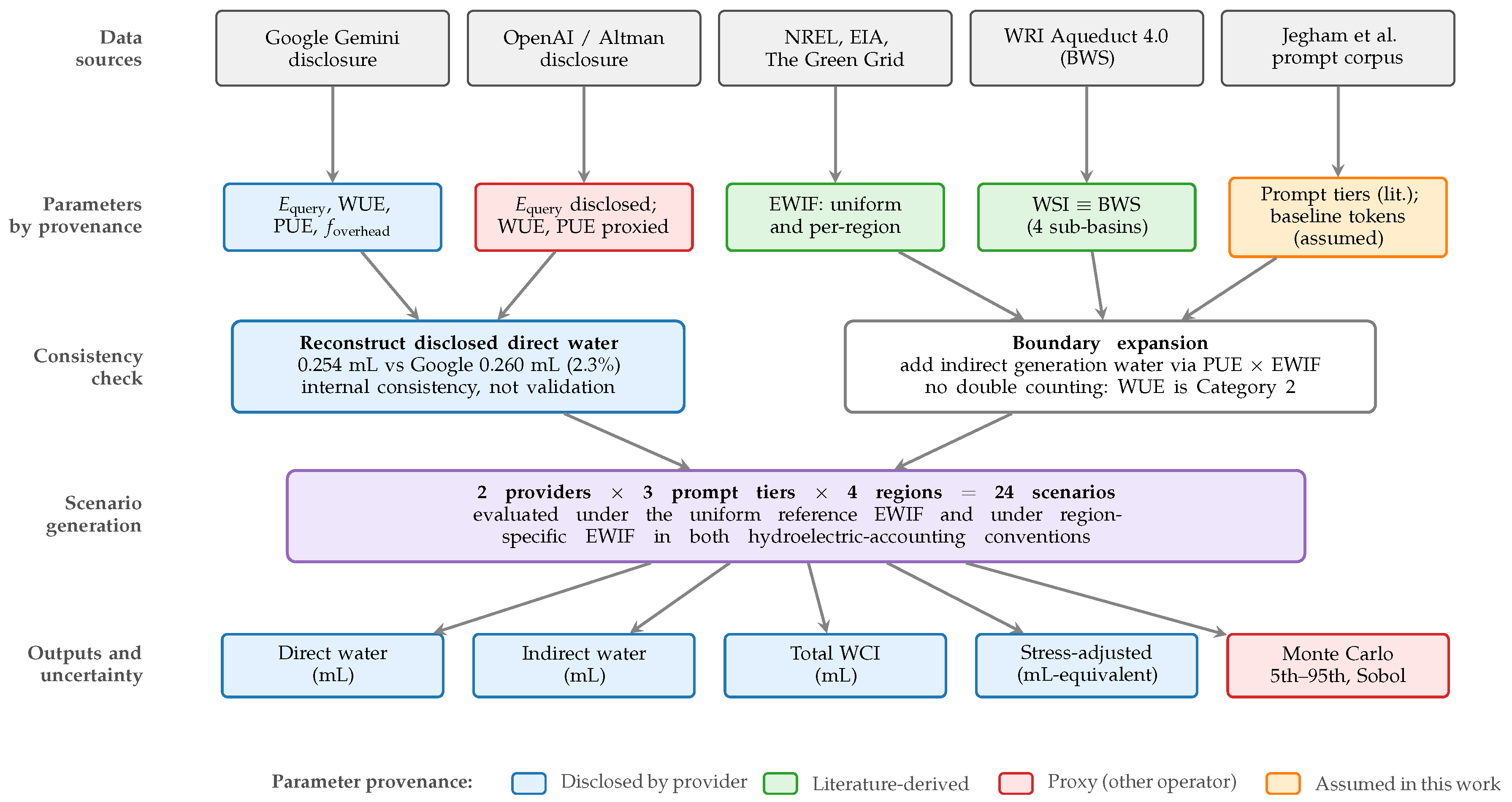
Table 1.
Core modeling parameters used in the WCI calculations, grouped by provenance. Disclosed values are published by the provider. Literature-derived values are taken from peer-reviewed or standards sources. Proxy values substitute another organization’s published figure where the provider discloses none. Assumed values are set in this work and are not reported by any source.
2.2. Components of the Direct-Water Accounting Boundary
Since WUE is reported as a single aggregate figure, it is worth stating explicitly which physical water flows it does and does not represent. Following the distinction drawn in the data-center water literature, withdrawal denotes water taken from a source, surface water, groundwater, reclaimed water, or treated potable supply, whereas consumption denotes water that is lost to that source, in cooling applications predominantly through evaporation [12]. WUE as defined in The Green Grid White Paper #35 and standardized in ISO/IEC 30134-9 is a consumption metric [9], and the direct-water term of WCI inherits that boundary.
Within a conventional evaporatively cooled facility, the water entering the cooling system is partitioned between distinct fates. The dominant consumptive term is evaporative loss from the cooling tower, the mechanism by which heat is actually rejected and irrecoverably lost to the local water body. A second fraction leaves the system as blowdown: because evaporation concentrates dissolved solids in the circulating loop, a portion of the circulating water must be bled off and replaced to maintain that concentration within limits set by the makeup-water chemistry and the system materials. Blowdown is a discharge rather than a consumption, and depending on local permitting it may be sent to sewer, treated on site, or recovered for reuse. Makeup water is then drawn to replace both evaporative losses and blowdown. A per-query metric built on WUE, therefore, captures evaporative consumption, but does not by itself distinguish a facility that discharges a large blowdown stream from one operating at higher cycles of concentration with a correspondingly smaller discharge [16].
The source of the makeup water is a further dimension that WUE does not express. A facility supplied with reclaimed or non-potable water may report the same WUE as one supplied from a treated potable network while placing a materially smaller burden on drinking-water supply, and potable sourcing remains common in reported data-center supply [12]. Two facilities with identical WUE can, therefore, carry appreciably different freshwater impacts. We treat this as a stated limitation of the direct-water term rather than as a property the metric resolves.
2.3. Cooling Technology and the WUE Term
The WUE values used in this paper are properties of particular cooling architectures, not of providers in the abstract. The near six-fold spread between Google’s reported 1.15 L/kWh and the 0.19 L/kWh hyperscale proxy adopted for OpenAI is best understood in those terms. Open-circuit evaporative cooling towers reject heat by evaporating water and, therefore, sit at the high-water, low-cooling-energy end of the design space. Closed-loop chilled-water systems with air-cooled condensers and fully dry or air-cooled designs approach zero on-site water consumption but raise facility electrical demand in order to reject the same heat load. Hybrid designs switch between the two modes seasonally, and direct liquid or immersion cooling changes the heat-capture path at the rack rather than the heat-rejection mechanism at the facility boundary [17]. The direction of this trade-off is well established in the data-center thermal-management literature [18,19,20]. The reported WUE also varies strongly with climate and site, so a fleet-average figure should not be read as characteristic of any individual facility [21].
This trade-off is precisely why a boundary-complete metric behaves differently from a direct-only one. Eliminating cooling-tower evaporation does not eliminate the water associated with serving a query; it relocates that water from the direct term, where it appears as on-site consumption, into the indirect term, where it appears as additional generation water arising from higher facility electricity demand. A direct-only disclosure records such a change as an unambiguous improvement, whereas WCI records the net effect, which may be favorable, unfavorable, or approximately neutral, depending on the EWIF of the serving grid. We regard this as the principal analytical argument for combining WUE, PUE, and EWIF within a single expression rather than reporting them separately.
2.4. Cooling-Water Quality, Treatment, and Discharge
The freshwater impact of data-center cooling is not fully described by volume alone because the water returned to the environment differs in quality from the water withdrawn. Since evaporation concentrates dissolved constituents in the circulating loop, cooling-water systems are operated under chemical treatment programs that control scale formation and corrosion and suppress biological growth, typically combining scale and corrosion inhibitors with biocidal dosing. The cycles of concentration achievable in practice are bounded by the hardness, alkalinity, and silica content of the makeup water, and blowdown discharged from such a system, therefore, carries elevated dissolved solids relative to the intake.
These practical aspects bear directly on how a per-query water figure should be interpreted. Cooling water returned to supply carries higher concentrations of calcium, chloride, and silica. These can affect the taste of drinking water, reduce crop yields, and prove toxic to aquatic organisms, and discharge of heated water and elevated salinity adds further ecological risk. Cooling towers that are inadequately maintained can also support the growth of Legionella, which may be dispersed in emitted water vapor [16]. Mitigation, therefore, extends beyond volumetric efficiency to source substitution and to the blowdown-handling options already introduced in Section 2.2 [22].
WCI, in common with WUE and with the per-query disclosures it reconstructs, is a volumetric metric and represents none of these quality dimensions. We include this discussion because the practical freshwater impact of a facility depends on them, and because a per-query volume should not be read as a complete characterization of that impact. Extending query-level accounting to water quality, thermal load, and source substitution would require facility-level discharge data that no provider currently publishes; we identify it as a direction for future work rather than presenting an estimate the available disclosures cannot support.
2.5. Data and Assumptions
The analysis uses public per-query disclosures for Google Gemini and OpenAI GPT-4o. Google reports median prompt energy and direct cooling water [7]. OpenAI reports average query energy and approximate water use but does not publish a comparable methodology [8]. Prompt tiers follow the Jegham et al. definitions: 400 tokens for short prompts, 2000 for medium prompts, and 11,500 for long prompts [14].
Grouping Table 1 in this way makes the asymmetry between the two providers explicit. Every parameter entering the Google scenarios is either disclosed by Google or taken from the literature, whereas two of the four facility parameters entering the OpenAI scenarios are proxies from another operator. The two baseline token counts are assumptions of this work and are reported here rather than only in the surrounding text, because they set the per-token rate on which every prompt-tier result depends. All WCI values reported in Section 3.2, Section 3.3 and Section 3.4 are calculated quantities derived from these inputs, and no reported WCI figure is itself a disclosed or measured value.
Three OpenAI parameters in Table 1 (WUE, PUE, and the facility-energy fraction implied by PUE) are proxies rather than disclosed measurements. OpenAI does not publish facility-level water-efficiency or power-efficiency figures for its inference infrastructure. We, therefore, adopt hyperscale-provider averages reproduced in the cross-vendor benchmarking literature: a WUE of 0.19 L/kWh and a PUE of 1.12, consistent with the AWS fleet values reported in Jegham et al. [14]. Two caveats apply. First, OpenAI’s actual hosting environment may differ from this proxy; published Microsoft fleet WUE values, for instance, are higher (approximately 0.30 L/kWh globally). We adopt the AWS values because they are documented within the same cross-vendor source used elsewhere in this paper and yield a conservative direct-water estimate. Second, 0.19 L/kWh is materially below the industry-average WUE of approximately 1.8 L/kWh [9], so the OpenAI direct-water estimates should be read as a lower bound on OpenAI’s actual on-site cooling water consumption. The indirect (EWIF) and stress-adjusted (WSI) factors applied to OpenAI scenarios are identical to those used for Google, thereby keeping cross-provider comparisons internally consistent within the framework, even though the underlying disclosure quality differs.
The EWIF value of 1.80 L/kWh warrants similar scrutiny. It is the thermoelectric figure reported by Torcellini et al., who estimate that approximately 0.47 gallons, or 1.8 L, of freshwater is evaporated per kWh delivered to the point of end use by thermoelectric generation [11]. Two features of that source qualify its use here. First, the same analysis reports a national weighted average of approximately 2.0 gallons, or 7.6 L, per kWh once hydroelectric generation is included alongside thermoelectric generation. The value adopted in the reference case is, therefore, a conservative lower bound on US grid-average generation water intensity rather than a central estimate. As the regional derivation below shows, however, it is not conservative with respect to the four specific sites examined here, each of which has a substantial share of non-thermal generation. Second, and more consequentially for the regional analysis, water generation intensity varies substantially with the grid mix: reservoir evaporation gives hydroelectric generation a far higher per-kWh water intensity than thermoelectric generation in the same source, and regional assessments confirm that per-kWh water consumption differs markedly across US regions and generation portfolios [6,23].
Because a single value cannot represent this variability, we parameterize EWIF by region. Each region’s EWIF is derived rather than assumed. The share of in-state net generation by fuel, taken from the EIA state electricity profiles for 2024, is weighted by the per-fuel consumptive intensities of The Green Grid White Paper #35 Table A-1 [9]. Those intensities are 2.20 L/kWh for wet-cooled coal, 3.30 L/kWh for nuclear, 0.80 L/kWh for combined-cycle natural gas, and zero for wind and solar photovoltaic generation. Biomass and petroleum steam cycles, which together account for less than 0.5% of generation in any region considered, are treated as wet-cooled thermal plants. The resulting values are reported in Table 2.
Table 2.
Region-specific EWIF derived from 2024 generation mix, under both hydroelectric-accounting conventions. The single value of 1.80 L/kWh used in the reference case is shown for comparison.
Hydroelectric generation requires a decision that the literature does not settle, and we, therefore, report two conventions rather than choosing one. Under the operational convention, reservoir evaporation is not allocated to electricity generation, and hydroelectric output is assigned zero consumptive intensity. Under the reservoir convention, gross reservoir evaporation is allocated to generation at 68 L/kWh [11]. We report the operational convention as the base case, because it matches the thermoelectric-average convention adopted in the data-center water literature [5,12] and is the more conservative claim, and the reservoir convention as an upper bound, because the dominant gross-evaporation method has been reviewed and found over-simplistic and potentially biased [24]. The single-EWIF results are retained throughout as a reference case so that the effect of regionalization is visible rather than absorbed.
Two results follow, and both revise how the regional analysis should be read. First, every region falls below 1.80 L/kWh under the operational convention. The uniform thermoelectric value is conservative when compared with the 7.60 L/kWh national average, which includes hydroelectric generation, but for these four particular sites, it overstates indirect water use because each has a substantial non-thermal share. Second, and more consequentially, the regional ordering reverses between the two conventions. Under the operational convention, Oregon is the least water-intensive grid of the four at 0.30 L/kWh; under the reservoir convention, it is the most water-intensive at 28.18 L/kWh, a factor of ∼94. No other region moves by more than a factor of three. The ordering of the remaining three regions is governed not by water stress but by nuclear share, which carries the highest per-kWh consumptive intensity of any generation type in that source [9]: Virginia and Arizona, at 30% and 27% nuclear, respectively, have the highest operational EWIF despite lying at opposite extremes of baseline water stress.
This is a methodological finding in its own right. A region cannot be characterized as water-intensive or water-efficient in electricity terms without first fixing the hydroelectric-accounting convention, and the choice is not a detail: for a hydro-dominated grid, it changes the answer by nearly two orders of magnitude. Reporting per-query water against a single grid-average intensity entirely conceals this.
Two objections to this result are worth pre-empting, because both can be settled from the numbers themselves.
The first is that the effect might be peculiar to Oregon, since no other region moves by more than a factor of three. It is not. The ratio between the two conventions is , where h is the hydroelectric share of generation, x the intensity assigned to hydroelectric output, and the operational EWIF. That expression reproduces all four regional swings exactly (93.9, 2.6, 2.9, and 1.4 for Oregon, Iowa, Arizona, and Virginia, respectively), so the magnitude of the swing is determined entirely by a region’s hydroelectric share relative to the water intensity of its thermal fleet. Oregon is not anomalous; it simply sits at the high end of a continuous relationship that every grid occupies. Any hydro-served region will exhibit the same behavior in proportion to .
The second is that the reversal depends on the specific value assigned to hydroelectric generation, which is the least settled quantity in this analysis. It does not. Solving for the intensity at which Oregon overtakes each of the other three regions gives 0.68 L/kWh for Iowa, 3.05 L/kWh for Arizona, and 3.08 L/kWh for Virginia. Oregon is, therefore, the most water-intensive grid of the four for any hydroelectric intensity above roughly 3.1 L/kWh, against the 68 L/kWh adopted here, a margin of more than twenty-fold. Published estimates of hydroelectric water consumption vary widely and are methodologically contested [24], but they do not vary within a range that could overturn the ordering. What the reversal depends on is the binary decision of whether reservoir evaporation is allocated to generation at all, not on the magnitude chosen once that decision is made. The magnitude governs only how large the swing is, not its direction.
2.6. Prompt-Tier Definition
The short, medium, and long tiers are set at 400, 2000, and 11,500 tokens, following Jegham et al. [14]. We adopt an externally published tiering rather than defining our own for a specific methodological reason: tier boundaries chosen by the same authors who report the results can be selected, consciously or not, to produce a preferred spread, and adopting a tiering fixed in a prior study removes that degree of freedom. The consequence is that the tiers are not tuned to this framework, and the boundaries should be read as representative prompt sizes drawn from an external corpus rather than as thresholds with physical meaning.
Two qualifications follow. First, because energy is scaled linearly from a single disclosed operating point, the tier boundaries set the spread of the reported results but not their central value: choosing different boundaries would rescale the short and long rows without altering the medium-tier estimate or any conclusion drawn from it. Second, the tiers count input tokens. Output length, which the inference-energy literature identifies as frequently dominant [25,26], is not represented in either provider’s published per-query figure and, therefore, cannot be tiered from the available disclosures.
2.7. Provider Coverage and Disclosure Triage
This study reports full estimates for two providers. Because that coverage is a consequence of what is disclosed rather than of what was examined, Table 3 records the disclosure status of every major provider assessed, including those that could not be included and the reason in each case.
Table 3.
Disclosure status of the providers assessed for inclusion. Status uses a fixed vocabulary: included where the disclosure supports an estimate, excluded where it does not, discussed only where a figure exists on a different accounting boundary, and not applicable where the provider does not operate the serving infrastructure. The reasons for exclusion differ: Microsoft Copilot discloses fleet facility parameters but no per-query workload; Meta Llama (version 3.1) is served by third parties as often as by Meta, so no single facility parameterization applies; Anthropic Claude and xAI Grok have no located disclosure; Mistral publishes a figure on a different boundary; and Perplexity routes queries to models operated by others.
The decision rule applied is stated so that it can be checked. A provider receives a point estimate only where both per-query energy and facility water efficiency are published for its own infrastructure. A provider with published energy but no facility parameters receives an interval that spans the plausible hyperscale range, presented as a scenario band rather than a single value. A provider with neither is excluded, and the gap is recorded here rather than filled by assumption. Extending the study to six further providers would have required proxying two or three parameters apiece, which multiplies precisely the weakness that the OpenAI scenario already exhibits: the uncertainty analysis of Section 3.4 shows that a single proxied WUE is enough to make two providers statistically indistinguishable. Adding providers on that basis would lengthen the results without strengthening them.
Two of the excluded cases are worth stating explicitly, because they are informative rather than merely absent. Microsoft publishes a fleet-average WUE of 0.27 L/kWh and a corresponding PUE [27], and Meta reports comparable figures for its own campuses [28]. For both, the facility half of the calculation is available. What is missing is a per-query energy figure for Copilot; for Llama the question is ill-posed, since the model is served by many operators with different facilities. The binding constraint for these providers is workload disclosure, not facility disclosure, which is the reverse of the OpenAI case and suggests that no single disclosure improvement would unlock cross-provider comparison on its own.
Perplexity is not a distinct case for a framework of this kind, because it routes queries to models operated by other providers. Its per-query water cost is that of whichever model served the request, plus a retrieval overhead. We note this because it identifies an attribution problem that the framework does not resolve: for routed or brokered services, the entity a user transacts with is not the entity whose facility consumes the water, and a per-query metric must specify which of the two it describes.
Mistral (Mistral Large 2) is the most instructive exclusion. It has published a full life-cycle assessment of Mistral Large 2, conducted under the AFNOR Frugal AI methodology with third-party review, reporting approximately 45 mL of water per response [29]. That figure is roughly two orders of magnitude above the full-boundary WCI estimates reported here, and the difference is almost entirely one of accounting boundary rather than of efficiency: the Mistral figure amortizes model training and hardware manufacture across inference requests, whereas WCI, like the Google and OpenAI disclosures it reconstructs, counts operational water only. The comparison is, therefore, not evidence that one service is thirstier than another. It is direct evidence for this paper’s central claim, that a per-query water figure is uninterpretable unless its boundary is stated, and it shows that the problem is already live in published industry disclosures rather than hypothetical.
3. Results
3.1. Reconstruction of the Disclosed Direct-Water Value
Google reports 0.24 Wh per median Gemini text prompt and 0.26 mL of direct on-site cooling water [7]. Applying the direct-water equation of Section 2.1 with Google’s WUE Category 2 value of 1.15 L/kWh and its reported 8% overhead exclusion gives:
This is within 0.006 mL, or approximately 2.3%, of Google’s 0.260 mL disclosure, reconstructing the published value from the published inputs. The 1.15 L/kWh figure is Google’s fleet-wide WUE reported in Section 3.3 of the Gemini technical paper [7]. “Category 2” refers to the on-site cooling-water accounting boundary defined in ISO/IEC 30134-9 and originally proposed in The Green Grid White Paper #35 [9]. It counts all freshwater consumed inside the facility for cooling, including cooling towers, evaporative cooling, and makeup water for the chilled-water loop. It excludes water consumed at upstream generation plants. That upstream water is captured separately by the EWIF term in the indirect-water equation, which is why our boundary expansion in subsequent sections recovers it without double-counting.
Table 4 sets the reconstruction against the published figure for both providers and, alongside it, the boundary-expanded estimate.
Table 4.
Published per-query water figures compared with the WCI reconstruction, at each provider’s own disclosed per-query energy (0.24 Wh for Gemini, 0.34 Wh for GPT-4o) and the reference EWIF of 1.80 L/kWh. The difference columns compare the public water figure with the WCI direct term only, since those two share the same on-site cooling boundary; the indirect and total columns lie outside that boundary and are given for context, not a comparison.
For Gemini, the same-boundary reconstruction agrees to 2.3%, while the boundary-complete total is 179% above the disclosure. The GPT-4o row is not a like-for-like test: OpenAI does not specify the accounting boundary of its published figure, and its WUE is a hyperscale proxy, so the apparent shortfall reflects an unknown boundary rather than a measured discrepancy. This calculation is a reconstruction rather than a validation. It uses Google’s own reported energy, WUE, overhead exclusion, and accounting boundary, so close agreement demonstrates that our implementation of the disclosed methodology is correct. That is an internal consistency check. External validation would require independently measured facility water data attributable to a known query volume, and no such measurement is publicly available for any commercial LLM deployment. We do not claim one. The value of the exercise is that it anchors the framework’s direct-water term to a published reference point before the accounting boundary is expanded, not that it establishes predictive accuracy.
3.2. WCI Scenario Results
We define the base experiment as the direct application of the WCI equations from Section 2.1 to the disclosed and proxy parameter values listed in Table 1, with no sensitivity perturbations and no water-stress adjustment applied. The base experiment evaluates 24 scenarios formed by the Cartesian product of two providers (Google Gemini and OpenAI GPT-4o), three prompt tiers (Short, Medium, Long), and four representative U.S. data-center regions (Oregon, Iowa, Virginia, Arizona). It serves as the reference point against which the regional stress adjustment of Section 3.3 and the EWIF sensitivity analysis of Section 3.4 are compared. Before stress adjustment, WCI is constant across regions for a given provider and prompt tier because the base case applies provider-level WUE and a single EWIF value to every region. Regional variation is introduced later through WSI.
Table 5 summarizes WCI by provider and prompt tier. Because neither provider discloses the exact token count behind its published per-query energy figure, we anchor each disclosure to an assumed baseline query length, 300 tokens for Google Gemini and 500 tokens for OpenAI GPT-4o, and derive a per-token energy rate by dividing each provider’s per-query energy by its baseline. That rate is then scaled to the 400-, 2000-, and 11,500-token short, medium, and long tiers to obtain the per-tier energy in Table 5, with the direct, indirect, and total water columns following from the WCI equations.
Table 5.
WCI summary by provider and prompt tier. Values are computed by applying the WCI equations to the parameters in Table 1, with per-token energy obtained by dividing each provider’s per-query disclosure by its assumed token count. All values are calculated scenario estimates, not measurements. Google values derive from disclosed facility parameters; OpenAI values derive from hyperscale proxies and should be read as an illustrative scenario.
This procedure assumes that per-query energy scales linearly with input token count, and that assumption warrants explicit justification. It is a simplification in at least three respects: attention cost grows superlinearly with sequence length; output length is frequently the dominant contributor to inference energy and is not represented in either provider’s published per-query figure; and batching, quantization, and model architecture all change the energy drawn per token [14,25,26]. We nevertheless adopt linear scaling because neither provider discloses the token count underlying its published energy value, so a constant per-token rate is the only scaling rule consistent with a single disclosed operating point. The prompt-tier results should, therefore, be read as first-order estimates that isolate the effect of prompt size under a fixed per-token assumption, rather than as measured energy profiles. Relaxing this assumption, in particular by modeling output length as a separate term, is identified in Section 5 as a priority for future work.
Figure 2 presents the two dimensions of Table 5 that are not readable from the numbers alone: the split of total WCI into its direct and indirect components, and the scaling of the total across prompt tiers. The component split is the substantive one. Scaling across tiers follows from the linear per-token assumption of the preceding paragraph and is shown for completeness rather than as a result.
Figure 2.
(a) Direct and indirect WCI components for medium prompts. Indirect electricity-generation water is the larger component for both providers under the uniform reference EWIF. (b) Total WCI across prompt tiers. The monotonic increase restates the linear per-token energy assumption and is not an independent finding.
3.3. Regional Scarcity-Adjusted Scenarios
Multiplying a physical volume by a 0–5 scarcity score treats environmental impact as linear and proportional in water stress. That is a modeling choice rather than a physical law, and it should be stated as one. The established alternative is the WULCA AWARE family of characterization factors, which are the LCA-standard approach and are non-linear in scarcity; we retain the Aqueduct score here because it is published at the sub-basin resolution the analysis requires, whereas substituting AWARE would change Equation (4) in form as well as in value. The framework itself is agnostic to the choice of index. Note also what does and does not vary regionally in what follows: EWIF is parameterized by regional generation mix, as set out in Section 2.5, and WSI varies by sub-basin, but WUE remains a single fleet value per provider because no provider publishes facility-level water efficiency by site. This section, therefore, reports scarcity-adjusted scenarios based on a partially regionalized physical estimate, rather than a full regional water-footprint assessment.
Physical water use does not fully describe environmental impact. The same volume of water has different significance in low-stress Oregon and high-stress Arizona. The framework, therefore, multiplies total WCI by WSI. We use site-specific WSI values obtained directly from the WRI Aqueduct 4.0 Water Risk Atlas [13], specifically the Baseline Water Stress (BWS) 0–5 score for each data-center sub-basin. The Aqueduct BWS score is used directly as the WSI term in Equation (4); that is, on Aqueduct’s 0–5 scale, with no rescaling, normalization, or transformation of any kind applied between the published score and the multiplier used here. BWS is defined by the World Resources Institute as the ratio of total water withdrawals to the available renewable surface and groundwater supplies within a sub-basin, binned onto the 0–5 scale, so that a higher score denotes greater competition for locally available freshwater [13]. WSI is used in this paper as the generic name for the scarcity weight in the framework, and BWS as the specific published dataset supplying its values; the framework itself is agnostic to the choice of index, and an alternative such as the WULCA AWARE characterization factor could be substituted without altering Equation (4). The four representative sites and their scores are: The Dalles, Oregon (Middle Columbia/Hood sub-basin), 0.000; Council Bluffs, Iowa (Big Papillion/Mosquito), 0.128; Ashburn/Loudoun County, Virginia (Middle Potomac/Catoctin), 0.158; and Mesa, Arizona (Lower Salt), 5.000. Three of the four hubs fall in Aqueduct’s “Low” category, with raw withdrawal-to-supply ratios below 6%; Mesa sits in a sub-basin where withdrawals exceed renewable supply by roughly 2.5×, which is the Aqueduct ceiling for “Extremely High” stress. We report stress-adjusted WCI in “mL-equivalent” to signal that it is a scarcity-weighted characterization metric, not a measure of additional physically evaporated water.
As a worked example, the Google Gemini medium-prompt scenario has mL (Table 5). Served from a data center in Mesa, Arizona (), this becomes
while the identical query served from Ashburn, Virginia (), yields 0.76 mL-equivalent, and from Council Bluffs, Iowa (), yields 0.62 mL-equivalent. All arithmetic is carried out at full precision and reported to two significant figures. The Dalles, Oregon (), yields mL-equivalent because the Columbia/Hood sub-basin has effectively no baseline water stress. The physical water draw is identical in all four cases; the order-of-magnitude differences reflect only the relative scarcity of freshwater at each location; Arizona is approximately 32× more stressed than Virginia and 39× more stressed than Iowa.
Applying the WSI values above to the base-case totals in Table 5 produces the stress-adjusted matrix in Table 6. Although the base-case totals are constant across regions, the stress-adjusted output forms a true 24-cell matrix because each (provider, tier) row is multiplied by four different WSI values, which makes the same physical water draw appear heavier in high-stress regions.
Table 6.
Stress-adjusted WCI (mL-equivalent) across all 24 provider–tier–region scenarios, computed as using Aqueduct 4.0 Baseline Water Stress scores for each sub-basin [13]. The Google values derive from disclosed facility parameters; the OpenAI values derive from hyperscale proxies and should be read as an illustrative scenario.
The same matrix is visualized as a heatmap in Figure 3. The color gradient confirms that Arizona dominates the regional pattern: because three of the four representative hubs sit in Aqueduct “Low” sub-basins, their stress-adjusted cells (Oregon, Iowa, Virginia) are barely visible relative to the saturated Arizona column. The regional scarcity story, therefore, collapses to a sharp Arizona-versus-the-rest contrast rather than a smooth gradient across all four locations.
Figure 3.
Stress-adjusted WCI (mL-equivalent) across the 24 provider–tier–region scenarios, with regional WSI taken from the Aqueduct 4.0 Baseline Water Stress sub-basin scores [13]. The figure visualizes the matrix tabulated in Table 6. Oregon (WSI 0.000), Iowa (0.128), and Virginia (0.158) appear near-zero on the color scale; only Arizona (WSI 5.000) shows saturated color, reflecting its position as the single high-stress outlier among the four representative data-center hubs.
The matrix above applies the reference EWIF, so its regional variation arises entirely from the WSI multiplier. Substituting the region-specific EWIF values of Table 2 allows physical consumption and scarcity weighting to be separated, and Figure 4 shows the derived intensities under both hydroelectric conventions.
Figure 4.
Regional parameterization of the indirect-water term. (a) Region-specific EWIF derived from 2024 generation mix, ordered from lowest to highest under each hydroelectric-accounting convention. The regional ordering reverses between conventions: Oregon is the least water-intensive grid under the operational convention and the most water-intensive under the reservoir convention, and every region falls below the uniform 1.80 L/kWh reference value under the operational convention. (b) Physical and scarcity-adjusted WCI by region for the Google Gemini medium prompt under both conventions and under the uniform reference value. Physical WCI is shown on a logarithmic axis. Oregon’s WSI of 0.000 maps every physical estimate, including the largest in the study, to zero mL-equivalent.
Panel (b) of the same figure reports the consequence for the Google Gemini medium-prompt case. Under regional EWIF and the operational convention, physical WCI ranges from 2.2 mL in Oregon to 4.4 mL in Virginia, against 4.8 mL under the uniform reference value: regionalization lowers the estimate everywhere, by 54% in Oregon and by 10% in Virginia. Under the reservoir convention, the range widens to 4.3 mL in Iowa and 51 mL in Oregon, with the latter being an order of magnitude above the reference case.
Reporting the two quantities side by side exposes a property of the framework that the reference case obscured. Oregon carries the highest physical water consumption of the four regions under the reservoir convention and the lowest under the operational one, yet in both cases, its scarcity-adjusted value is exactly zero, because Aqueduct assigns the Middle Columbia/Hood sub-basin a Baseline Water Stress score of 0.000. A linear multiplier with a zero floor, therefore, maps an unbounded physical quantity to zero whenever local stress is negligible. We regard this as a property to be stated rather than concealed: a stress-adjusted value of zero denotes the absence of local scarcity, not the absence of water consumption, and the two quantities must, therefore, be reported together. This is also an argument for characterization factors that do not vanish at low stress, such as the WULCA AWARE factors discussed in Section 5, and it is the clearest illustration in this study of why physical and scarcity-weighted water should not be collapsed into a single reported number.
Because the verified Aqueduct 4.0 scores place three of the four sub-basins inside the “Low” band, the scarcity axis does not form a smooth gradient: Arizona stands as a single high-stress outlier with the other three sites clustered near zero. The regional set, therefore, exercises the physical dimension of the framework more fully than the scarcity dimension, a limitation we return to in Section 5.
3.4. Uncertainty and Parameter Influence
Varying a single parameter characterizes the model rather than the uncertainty. Sweeping EWIF alone across its plausible range traces a straight line because Equation (2) is linear in EWIF; the exercise recovers the slope that was assumed and adds no information about how confident a reader should be in any reported value. We, therefore, propagate uncertainty through every input simultaneously and then decompose the resulting spread to establish which inputs are responsible for it.
Each parameter is assigned a distribution as follows: The disclosed quantities receive narrow triangular distributions centered on the published figure, reflecting that a fleet median is not a per-query constant. The two assumed baseline token counts follow uniform distributions, since no value is published, and none is more defensible than the others within the stated bounds. The OpenAI WUE receives a log-uniform distribution spanning the AWS proxy floor of 0.19 L/kWh to the industry average of 1.80 L/kWh, which represents the genuine state of knowledge for a provider that discloses nothing: the proxy is a lower bound rather than an estimate. EWIF is given a triangular distribution spanning the hydro-exclusive and hydro-inclusive accounting conventions discussed in Section 2.5. We draw independent samples under a fixed seed. Independence is itself an assumption, and a conservative one in this context: WUE and PUE are plausibly correlated in a real facility, since both reflect cooling-system design, and correlated draws, would narrow the intervals reported below. The overhead fraction is held fixed rather than sampled. For Gemini, it is a disclosed value, and for GPT-4o, it is set to zero as a refusal to assume an undisclosed exclusion rather than as an estimate of one; sampling it across its full plausible range of 0 to 0.12 moves the GPT-4o total by 0.006 mL, which is 0.4% of the width of the interval reported below and some seventy times smaller than the effect of the WUE proxy range already sampled. Including it would add a parameter requiring justification without changing any reported result.
Figure 5 shows the resulting distributions. The intervals are wide relative to the separation between the providers: the 5th–95th percentile bands overlap by roughly 95% at every prompt tier, and the probability that a Gemini query consumes more water than a GPT-4o query is close to even. The deterministic Gemini estimate sits near the middle of its own distribution, whereas the GPT-4o estimate sits near the 22nd percentile, reflecting that its proxy WUE is drawn from the low end of the plausible hyperscale range. Provider ranking is, therefore, not supported at the precision the point estimates appear to offer.
Figure 5.
Monte Carlo uncertainty in total WCI per query across 10,000 draws, by provider and prompt tier. Bars span the 5th to 95th percentile, filled circles mark the Monte Carlo median, and open diamonds mark the deterministic base case reported in Table 5. The two providers’ intervals overlap across 95% of their combined range at every prompt tier.
Two results follow, and both bear directly on how the scenario estimates of Section 3.2 should be read.
First, the deterministic base case sits in a different place within its own uncertainty distribution for each provider. For Google Gemini, it falls at the 56th percentile, close to the center, which is what one expects when every input is either disclosed or drawn from the literature. For OpenAI GPT-4o, it falls at the 22nd percentile. The published point estimate is, therefore, not a central case for OpenAI but a low one, and the reason is structural rather than incidental: the AWS proxy WUE of 0.19 L/kWh sits at the bottom of the plausible range for a provider whose facility water efficiency is undisclosed. Adopting the proxy as a point value understates the expected direct-water term, and the paper’s OpenAI figures should be read accordingly.
Second, and more consequentially, the two providers do not separate once uncertainty is propagated. The 90% intervals overlap across 95% of their combined range at every prompt tier, and the probability that a Gemini query consumes more total water than a GPT-4o query under these distributions is 0.52, which is indistinguishable from a coin flip. The apparent ordering in Table 5, in which Gemini shows a higher total WCI than GPT-4o at every tier, is an artifact of adopting a low proxy WUE for one provider and a disclosed value for the other. It is not a finding about the two services. This is the quantitative form of the caveat stated in Section 2.5, and it is the reason the cross-provider comparison in this paper is presented as an illustrative scenario rather than as a result.
Figure 6 decomposes the spread. For Google Gemini, the assumed baseline token count is the dominant contributor, accounting for 51% of output variance, with EWIF second at 33% and per-query energy third at 11%. WUE and PUE together account for less than 1%. For OpenAI GPT-4o the ordering shifts: EWIF and the baseline token count contribute 33% each, per-query energy 19%, and WUE 8%. Total-order indices exceed first-order indices only marginally, and first-order effects sum to 0.95 and 0.93 for the two providers, so interactions between parameters are weak, and the variance is close to additive in the individual inputs. The two panels rank the top two parameters differently. The reason is instructive rather than contradictory. The tornado moves each parameter between fixed percentile bounds and reports the widest achievable swing, which EWIF wins because its plausible range is the broadest. The Sobol indices instead weight each parameter by how much output variance it explains under its own distribution, which the baseline token count wins because a uniform prior over an undisclosed quantity places more mass away from the center. The first asks how far a parameter could move the answer; the second asks how much of the spread it causes. Both are reported.
Figure 6.
Relative influence of each input parameter on total WCI for the medium prompt tier. Left: one-at-a-time swing between the 5th and 95th percentile of each parameter, holding the others at their base values, with the vertical line marking the base case. Right: Sobol first-order () and total-order () variance contributions, estimated from a scrambled Sobol sequence using the Saltelli first-order and Jansen total-order estimators.
The practical reading of this decomposition is uncomfortable but useful. The parameter that most strongly governs the reported numbers, for Google, is not a physical property of any data center; it is our own assumption about how many tokens sit behind a disclosed per-query energy figure. Neither provider publishes that number. A single additional line in either disclosure, the token count underlying the published energy value, would remove more uncertainty from per-query water accounting than any improvement in facility-level water reporting. This is a specific and actionable disclosure recommendation, and we regard it as one of the more useful outputs of the framework.
Throughout the paper, we retain the deterministic base case as the central estimate rather than substituting the Monte Carlo median, and the two differ, most visibly for OpenAI, where the median exceeds the point estimate for the reason given above. The deterministic value is the one that traces line by line to published disclosures and can be recomputed by a reader from Table 1; the Monte Carlo supplies the interval around it. Reported values, therefore, take the form of a central estimate followed by a 5th-to-95th-percentile range, and we quote them to two significant figures, since the underlying inputs do not support more.
4. Discussion
WCI reproduces Google’s direct-water value to within 2.3%. That establishes that the framework correctly implements the disclosed accounting methodology, not that it accurately predicts facility water use. The results that follow are of more interest. Indirect electricity-generation water is not a small correction, although its share proves to be region-dependent once EWIF is parameterized by generation mix. Under the uniform reference EWIF, it accounts for approximately 65% of Gemini WCI and 91% of GPT-4o WCI. Under region-specific EWIF and the operational hydroelectric convention, the Gemini share falls to 61% in Virginia and 60% in Arizona but to 37% in Iowa and 24% in Oregon, so that in the two least thermally intensive grids the direct cooling term is the larger of the two. For GPT-4o, the indirect share remains dominant everywhere, between 66% and 91%, because its proxy WUE of 0.19 L/kWh leaves little direct water to compete with. The generalization that indirect water dominates per-query freshwater consumption, therefore, holds for the US thermoelectric average and for facilities with low on-site water intensity, but not universally: whether the direct or the indirect term dominates depends jointly on the cooling architecture of the facility and the generation mix of the grid serving it. This dependence is not visible when a single grid-average EWIF is applied, and we regard it as one of the more useful results the framework yields. Finally, when site-specific WSI values are drawn directly from Aqueduct 4.0 [13], the regional story is not a smooth gradient but a sharp outlier pattern: Mesa, Arizona (BWS 5.000) is roughly 32× more scarcity-weighted than Ashburn, Virginia (BWS 0.158) and 39× more than Council Bluffs, Iowa (BWS 0.128); against The Dalles, Oregon (BWS 0.000), the contrast is theoretically the maximum the Aqueduct 0–5 scale can express, since Arizona sits at the scale’s ceiling and Oregon at its floor. Three of the four major US data-center hubs we examined fall in Aqueduct’s “Low” category at the sub-basin level, which makes Arizona an outlier rather than a high end of a continuum.
The framework does not claim that stress-adjusted water is physically evaporated water. Rather, stress adjustment is a characterization step that expresses the severity of physical water consumption under local scarcity conditions. This distinction is essential for interpreting WCI responsibly.
Of these, the hydroelectric-accounting result is the one that was not assumed at the outset: it emerges from the interaction of independently sourced inputs, the per-fuel water intensities and each region’s generation mix, rather than being asserted as a modeling choice, and it is not a restatement of the model’s structure. It arises because the framework carries the generation-mix term explicitly: a grid can be the least water-intensive of a set under one defensible convention and the most water-intensive under another, and the choice between conventions is unsettled in the literature [24]. The practical consequence is that a per-query water figure is not comparable across studies unless the hydroelectric convention is stated alongside it, in the same way that a carbon figure is not comparable unless market-based or location-based accounting is specified. We are not aware of any existing per-query water disclosure that states this, and we regard establishing the requirement as a contribution of the present work.
Placing these results against the existing literature clarifies what the per-query resolution adds. Aggregate projections put global AI freshwater withdrawal at 4.2–6.6 billion m3 by 2027 [2], and reconciliation work has shown how widely published AI water estimates diverge once boundaries and assumptions are made explicit [3]. Those studies operate on fleets and years; WCI decomposes the same quantity to the level of an individual inference, which is the level at which routing, model selection, and procurement decisions are actually taken. Facility-level and geospatial water footprinting resolves where water is consumed [4,5] but not what a unit of service costs, and the EWIF values we inherit come from that literature [11,12]; our uniform reference value of 1.80 L/kWh is conservative relative to the hydro-inclusive national average reported in the same sources. We do not present WCI as a life-cycle assessment. It omits embodied water in hardware and construction, uses a linear characterization factor rather than an LCA-compliant one, and covers a single life-cycle stage, so the standards applied to LCA studies [30] should not be read as satisfied here.
Three practical uses follow, each bounded by the uncertainty quantified in Section 3.4. For sustainability reporting, WCI gives providers a boundary-complete per-query figure to publish alongside energy, comparable across vendors in a way that direct-only cooling water is not. The caveat is that a figure computed from proxy facility parameters carries an interval wide enough to overlap competitors. Such a disclosure is only as useful as the parameters behind it. For siting and workload routing, the Arizona-versus-Oregon contrast is a routing argument: identical computational work carries a scarcity weight of zero in one sub-basin and five in another. The regional EWIF results show the physical estimate moving in the opposite direction from the scarcity weight. The two must, therefore, be reported together rather than combined into a single ranking. For procurement and model selection, a buyer can, in principle, price water alongside cost and latency; the honest caveat is that our own uncertainty analysis shows that the two providers studied here are not separable on current disclosure, so the framework is at present better suited to comparing deployment configurations of a known facility than to comparing vendors.
The accounting structure generalizes beyond water, and the generalization is worth stating because it identifies what is specific to freshwater and what is not. The chain used here converts a workload quantity into a facility quantity via PUE, then into a resource quantity via an intensity factor, and finally into an impact-weighted quantity via a local characterization factor. Only the intensity factor and the characterization factor are water-specific. Substituting an air-side heat-rejection term for WUE yields a per-query estimate of the air throughput and sensible heat load of a dry-cooled facility, which is the natural counterpart metric for the arid-site designs that trade water for electricity; the same substitution makes the direct-to-indirect relocation described in Section 2 quantifiable rather than merely directional. Substituting land area or an embodied-materials intensity for the same term, amortized over hardware lifetime, extends the chain to the footprint categories excluded here. The same boundary-aware logic extends beyond resource accounting to the socio-technical design of the infrastructures that consume these resources, such as carbon-constrained supply-chain resilience [31]. What does not generalize is the characterization step: a scarcity weight is meaningful for water because freshwater availability is local, and it has no counterpart for a globally mixed quantity such as carbon, which is why the carbon framework that this work extends [1] requires no regional weighting term.
5. Limitations
We separate the limitations that affect the precision of the reported numbers from those that affect whether a conclusion holds at all because the two carry different consequences for a reader deciding how much weight to place on a given result.
5.1. Limitations Affecting Numerical Precision
Neither provider discloses the token count behind its published per-query energy figure, so the baseline token counts of Table 1 are assumptions of this work. The Sobol analysis of Section 3.4 identifies this as the single largest contributor to output variance for Google Gemini. Neither provider discloses output length either, which the inference-energy literature identifies as a major determinant of per-query energy [25,26]; the linear per-token scaling adopted in Section 3.2, therefore, captures the effect of prompt size but not that of response length. The regional EWIF parameterization is derived from the annual state-level generation mix rather than from the balancing-authority dispatch actually serving each facility. It, therefore, does not capture power purchase agreements, interstate transfers, or time-of-day variation in the marginal generator. It also uses fleet-average per-fuel intensities rather than plant-specific cooling configurations, which matters most for natural gas, where wet and dry cooling differ by roughly a factor of five. The Monte Carlo draws parameters independently, whereas WUE and PUE are plausibly correlated in a real facility; correlated sampling would narrow the reported intervals. Each of these affects how many significant figures a reported value supports. Directional robustness has been demonstrated explicitly only for the hydroelectric-convention finding, in Section 2.5; for the remaining items, we have not tested it, and cannot comment on whether it holds.
5.2. Limitations Affecting the Validity of Conclusions
The OpenAI WUE and PUE are proxies borrowed from another operator, and this does more than widen an interval: it invalidates the ranking, not merely its magnitude. Section 3.4 shows the two providers’ 90% intervals overlapping across 95% of their combined range, so no conclusion of the form “provider A consumes more water per query than provider B” is supported by this analysis. Any such reading of Table 5 would be an error.
No result here has been validated against independently measured facility water data, because no such measurement is publicly available for any commercial LLM deployment. The reconstruction in Section 3.1 establishes internal consistency with a disclosed methodology and nothing beyond that.
The hydroelectric-accounting convention remains unresolved in the literature rather than by this work. We report both bounds because the evidence does not support choosing between them, and any single-figure regional EWIF for a hydro-dominated grid should be treated as convention-dependent. We note, however, that the ordering result of Section 2.5 is not hostage to this. It requires only that hydroelectric generation be assigned an intensity above roughly 3.1 L/kWh, some twenty times below the value adopted here, so no plausible revision of the disputed magnitude would overturn it. What remains genuinely unsettled is whether the allocation should be made at all, and the absolute values under the reservoir convention, not the relative ordering they produce.
Treating WSI as a linear multiplier is a modeling choice, and its most consequential consequence is at the boundary: a Baseline Water Stress score of zero drives the scarcity-adjusted value to zero irrespective of physical consumption. Oregon carries the largest physical water estimate in this study under the reservoir convention and a scarcity-adjusted value of exactly zero. Physical and scarcity-adjusted quantities must, therefore, be read together, and a WULCA AWARE characterization factor, which does not vanish at low stress, would be the LCA-compliant alternative.
The four US sub-basins evaluated here do not span the global range of water-stress conditions: three fall in Aqueduct’s “Low” band, so the scarcity dimension of the framework is exercised by a single site. Widening the regional set requires Baseline Water Stress values read at sub-basin resolution for each candidate facility, matched to the specific catchment containing it. Country-level rankings are not interchangeable with sub-basin scores, and substituting them would introduce an inconsistency more damaging than the present narrow coverage, so the analysis is reported on the four sites the available sub-basin data support. Extending it to sites spanning the full stress range, including hyperscale clusters in arid regions outside the United States, is the highest-priority extension of this work; in the interim, the sensitivity results of Section 3.4 indicate how much of the reported variation is attributable to the scarcity weighting.
Finally, the analysis covers operational water consumption only and excludes embodied water in hardware manufacturing, data-center construction, and supply chains, so a WCI value is not a life-cycle water footprint and should not be compared with one.
A further limitation concerns what the framework measures about the prompt. The tiers of Section 2.6 vary the prompt length only, so the analysis cannot distinguish a long retrieval-style prompt from a short prompt requiring multi-step reasoning, and it is plausible that the response time and computational complexity track the latter more closely than the former. Testing this would require a controlled experiment measuring time-to-first-token and completion time across a factorial prompt set of matched lengths and differing complexity, repeated across load conditions, and we regard it as a valuable extension. We have not attempted it here for a reason that is methodological as well as practical: latency is not energy, and without hardware-level power telemetry, which no commercial API exposes, wall-clock time cannot be converted into the energy term the framework requires. Reporting a latency-derived water figure would introduce a conversion less defensible than the linear token assumption it was intended to replace. The experiment is, therefore, recorded here as the principal workload-side extension of this work, alongside the output-length term identified above, and both would be addressed by the same instrumented deployment.
Taken together, the finding that is robust is the boundary-gap result: adding electricity-generation water raises the per-query estimate substantially above the direct-only disclosure, and that conclusion rests only on Google’s disclosed parameters and on published generation-water intensities. The findings that are illustrative are all of those comparing providers.
6. Conclusions
WCI extends query-level AI sustainability accounting from carbon to freshwater consumption. The framework first reproduces Google’s publicly disclosed direct cooling-water figure, then expands the accounting boundary to include electricity-generation water and regional scarcity. The central finding is that direct-only reporting can be accurate within its own boundary while still understating the broader freshwater cost of inference: for Google’s disclosed median prompt, adding the indirect electricity-generation component raises the per-query estimate from the disclosed 0.260 mL to 0.725 mL, an increase of 179%.
The principal technical uncertainties are concentrated in three parameters. The EWIF carries the widest uncertainty of any term in the framework. Regionalizing it by generation mix lowers the medium-prompt estimate by 10% to 54% across the four sites under the operational hydroelectric convention, while the reservoir convention raises the Oregon estimate by an order of magnitude. The literature does not settle which convention is correct. The baseline token counts that anchor each provider’s per-query energy to prompt length are assumptions of this work rather than disclosed quantities, and they scale every prompt-tier result proportionally. Finally, the WUE and PUE values used for OpenAI are proxies from another operator, because OpenAI publishes neither; the OpenAI direct-water estimates should, therefore, be read as a lower bound, and the cross-provider comparison should be read as an illustrative scenario rather than a measured difference. Results derived from Google’s disclosed parameters and results derived from proxy values are not of equal evidential standing, and we have marked the distinction throughout.
For data-center water management, the framework’s practical implication is that direct-only water reporting can reward a change that does not reduce total freshwater consumption. Because dry and air-cooled designs reject the same heat load at higher electrical demand, replacing evaporative cooling reduces on-site consumption while increasing generation water; whether the net effect is an improvement depends on the water intensity of the serving grid, which a direct-only metric cannot express. The same logic applies to siting and workload routing: identical computational work carries materially different freshwater significance depending on both the generation mix and the baseline water stress of the receiving sub-basin. A boundary-complete per-query metric brings these trade-offs into a single accounting framework, expressed in comparable physical and scarcity-weighted terms rather than collapsed into one ranking, which is the capability that the integration of WUE, PUE, EWIF, and WSI is intended to provide.
Future work should address the framework’s parameterization in five directions. Site-specific WUE would replace fleet averages, which conceal substantial variation across facilities and climates. Region-specific EWIF, introduced in this work from annual state-level generation mix, should be refined to dispatch-resolved intensities that reflect the generator actually serving each facility at each hour, and the hydroelectric-accounting convention needs resolution in the wider literature before a single regional figure can be reported for a hydro-dominated grid. Cooling-technology scenarios would allow the direct-to-indirect water trade-off between evaporative, hybrid, and dry designs to be quantified rather than described. Alternative water sources, in particular reclaimed and non-potable supply, require accounting that distinguishes freshwater burden from total water throughput, which WUE alone does not. Water reuse, including on-site treatment and recovery of cooling-tower blowdown, would extend the boundary beyond the consumption-only convention adopted here. Beyond parameterization, independent measurement against facility-level water data remains the principal outstanding validation step, and none of the results reported here should be understood as substituting for it.
Author Contributions
Conceptualization B.S., R.K., K.M.P., E.P. and A.T.; methodology B.S., R.K. and A.T.; software, A.T.; validation, R.K. and A.T.; formal analysis, A.T.; investigation B.S., R.K., and A.T.; writing—original draft preparation, A.T.; writing—review and editing, B.S., R.K., K.M.P. and E.P.; supervision, K.M.P. and E.P. All authors have read and agreed to the published version of the manuscript.
Funding
This research received no external funding.
Institutional Review Board Statement
Not applicable.
Informed Consent Statement
Not applicable.
Data Availability Statement
The calculations, figures, and source code that reproduce the results are publicly available at https://github.com/anacodicAI-labs/hidden-thirst (last accessed 29 June 2026).
Conflicts of Interest
The authors declare no conflicts of interest.
References
- Kaur, R.; Kundu, T.; Park, K.M.; Pinsky, E. The Carbon Cost of Intelligence: A Domain-Specific Framework for Measuring AI Energy and Emissions. Energies 2026, 19, 642. [Google Scholar] [CrossRef] [Scilit]
- Li, P.; Yang, J.; Islam, M.A.; Ren, S. Making AI Less Thirsty: Uncovering and Addressing the Secret Water Footprint of AI Models. Commun. ACM 2025. [Google Scholar] [CrossRef] [Scilit]
- Ren, S.; Tomlinson, B.; Black, R.W.; Torrance, A.W. Reconciling the contrasting narratives on the environmental impact of large language models. Sci. Rep. 2024, 14, 26310. [Google Scholar] [CrossRef] [Scilit] [PubMed]
- Lei, N.; Lu, J.; Cheng, Z.; Cao, Z.; Shehabi, A.; Masanet, E. Geospatial assessment of water footprints for hyperscale data centers in the United States. Environ. Res. Lett. 2025, 20, 024011. [Google Scholar] [CrossRef] [Scilit]
- Siddik, M.A.B.; Shehabi, A.; Marston, L. The Environmental Footprint of Data Centers in the United States. Environ. Res. Lett. 2021, 16, 064017. [Google Scholar] [CrossRef] [Scilit]
- Chini, C.M.; Djehdian, L.A.; Lubega, W.N.; Stillwell, A.S. Virtual water transfers of the US electric grid. Nat. Energy 2018, 3, 1115–1123. [Google Scholar] [CrossRef] [Scilit]
- Elsworth, C.; Huang, K.; Patterson, D.; Schneider, I.; Sedivy, R.; Goodman, S.; Townsend, B.; Ranganathan, P.; Dean, J.; Vahdat, A.; et al. Measuring the Environmental Impact of Delivering AI at Google Scale. arXiv 2025, arXiv:2508.15734. [Google Scholar]
- Altman, S. The Gentle Singularity. 2025. Available online: https://blog.samaltman.com/the-gentle-singularity (accessed on 10 August 2026).
- The Green Grid. Water Usage Effectiveness (WUE): A Green Grid Data Center Sustainability Metric; Technical Report White Paper 35; The Green Grid: Washington, DC, USA, 2011. [Google Scholar]
- Avelar, V.; Azevedo, D.; French, A. (Eds.) PUE: A Comprehensive Examination of the Metric; Technical Report White Paper 49; The Green Grid: Washington, DC, USA, 2012. [Google Scholar]
- Torcellini, P.; Long, N.; Judkoff, R. Consumptive Water Use for U.S. Power Production; Technical Report NREL/TP-550-33905; National Renewable Energy Laboratory: Golden, CO, USA, 2003.
- Mytton, D. Data Centre Water Consumption. npj Clean Water 2021, 4, 11. [Google Scholar] [CrossRef] [Scilit]
- World Resources Institute. Aqueduct 4.0 Water Risk Atlas. Baseline Water Stress Indicator, Sub-Basin Scores. 2023. Available online: https://www.wri.org/applications/aqueduct/water-risk-atlas/ (accessed on 28 June 2026).
- Jegham, N.; Abdelatti, M.; Koh, C.Y.; Elmoubarki, L.; Hendawi, A. How Hungry is AI? Benchmarking Energy, Water, and Carbon Costs of AI Models. arXiv 2025, arXiv:2505.09598. [Google Scholar]
- Google. Google 2025 Environmental Report. 2025. Available online: https://www.gstatic.com/gumdrop/sustainability/google-2025-environmental-report.pdf (accessed on 10 August 2026).
- Khatib, L.; Pham, A.; Ahmed, K.; Frenkel, V.S. Data Centers and Water: Challenges and Solutions for Sustainable Cooling. J. AWWA 2025, 117, 48–53. [Google Scholar] [CrossRef] [Scilit]
- Ristic-Smith, A.; Rogers, D.J. Compact two-phase immersion cooling with dielectric fluid for PCB-based power electronics. IEEE Open J. Power Electron. 2024, 5, 1107–1118. [Google Scholar] [CrossRef] [Scilit]
- Nadjahi, C.; Louahlia, H.; Lemasson, S. A review of thermal management and innovative cooling strategies for data center. Sustain. Comput. Inform. Syst. 2018, 19, 14–28. [Google Scholar] [CrossRef] [Scilit]
- Habibi Khalaj, A.; Halgamuge, S.K. A Review on Efficient Thermal Management of Air- and Liquid-Cooled Data Centers: From Chip to the Cooling System. Appl. Energy 2017, 205, 1165–1188. [Google Scholar] [CrossRef] [Scilit]
- Moazamigoodarzi, H.; Tsai, P.J.; Pal, S.; Ghosh, S.; Puri, I.K. Influence of cooling architecture on data center power consumption. Energy 2019, 183, 525–535. [Google Scholar] [CrossRef] [Scilit]
- Shumba, N.; Tshekiso, O.; Li, P.; Fanti, G.; Ren, S. A water efficiency dataset for African data centers. In Proceedings of the NeurIPS Workshop on Tackling Climate Change with Machine Learning, Vancouver, BC, Canada, 15 December 2024. [Google Scholar]
- Ristic, B.; Madani, K.; Makuch, Z. The water footprint of data centers. Sustainability 2015, 7, 11260–11284. [Google Scholar] [CrossRef] [Scilit]
- Lee, U.; Han, J.; Elgowainy, A.; Wang, M. Regional water consumption for hydro and thermal electricity generation in the United States. Appl. Energy 2018, 210, 661–672. [Google Scholar] [CrossRef] [Scilit]
- Bakken, T.H.; Killingtveit, Å.; Engeland, K.; Alfredsen, K.; Harby, A. Water consumption from hydropower plants—Review of published estimates and an assessment of the concept. Hydrol. Earth Syst. Sci. 2013, 17, 3983–4000. [Google Scholar] [CrossRef] [Scilit]
- Desislavov, R.; Martínez-Plumed, F.; Hernández-Orallo, J. Trends in AI inference energy consumption: Beyond the performance-vs-parameter laws of deep learning. Sustain. Comput. Inform. Syst. 2023, 38, 100857. [Google Scholar] [CrossRef] [Scilit]
- Stojkovic, J.; Zhang, C.; Goiri, I.; Torrellas, J.; Choukse, E. DynamoLLM: Designing LLM inference clusters for performance and energy efficiency. In Proceedings of the IEEE International Symposium on High-Performance Computer Architecture (HPCA), Las Vegas, NV, USA, 1–5 March 2025. [Google Scholar]
- Microsoft. Measuring Energy and Water Efficiency for Microsoft Datacenters; Technical Report; Reported Fleet-Average Water Usage Effectiveness; Microsoft Corporation: Redmond, WA, USA, 2025. [Google Scholar]
- Meta Platforms. Data Centers: Water Stewardship and Efficiency; Technical Repor; Meta Platforms, Inc.: Menlo Park, CA, USA, 2025. [Google Scholar]
- Mistral AI. Our Contribution to a Global Environmental Standard for AI: Life Cycle Analysis of Mistral Large 2; Technical Report; Life-Cycle Assessment Conducted Under the AFNOR Frugal AI Methodology with Third-Party Review; Mistral AI: Paris, France, 2025. [Google Scholar]
- Schneider, I.; Xu, H.; Benecke, S.; Patterson, D.; Huang, K.; Ranganathan, P.; Elsworth, C. Life-cycle emissions of AI hardware: A cradle-to-grave approach and generational trends. arXiv 2025, arXiv:2502.01671. [Google Scholar]
- Kaur, R.; Kundu, T.; Sharma, B.; Park, K.M.; Pinsky, E. Operational Resilience Under Carbon Constraints: A Socio-Technical Multi-Agentic Approach to Global Supply Chains. Systems 2026, 14, 374. [Google Scholar] [CrossRef] [Scilit]
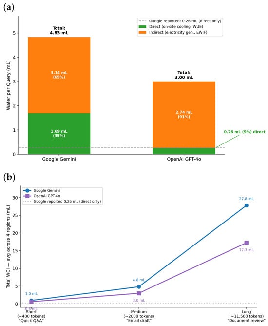
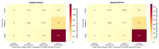
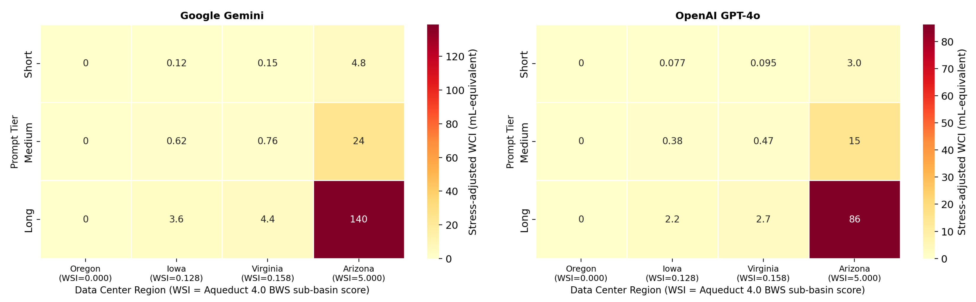
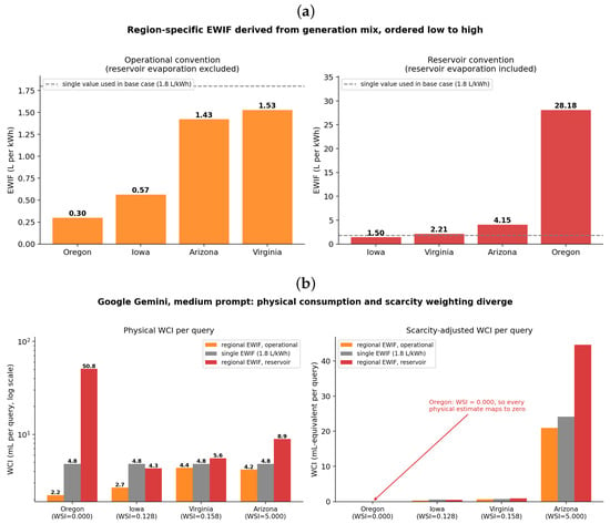
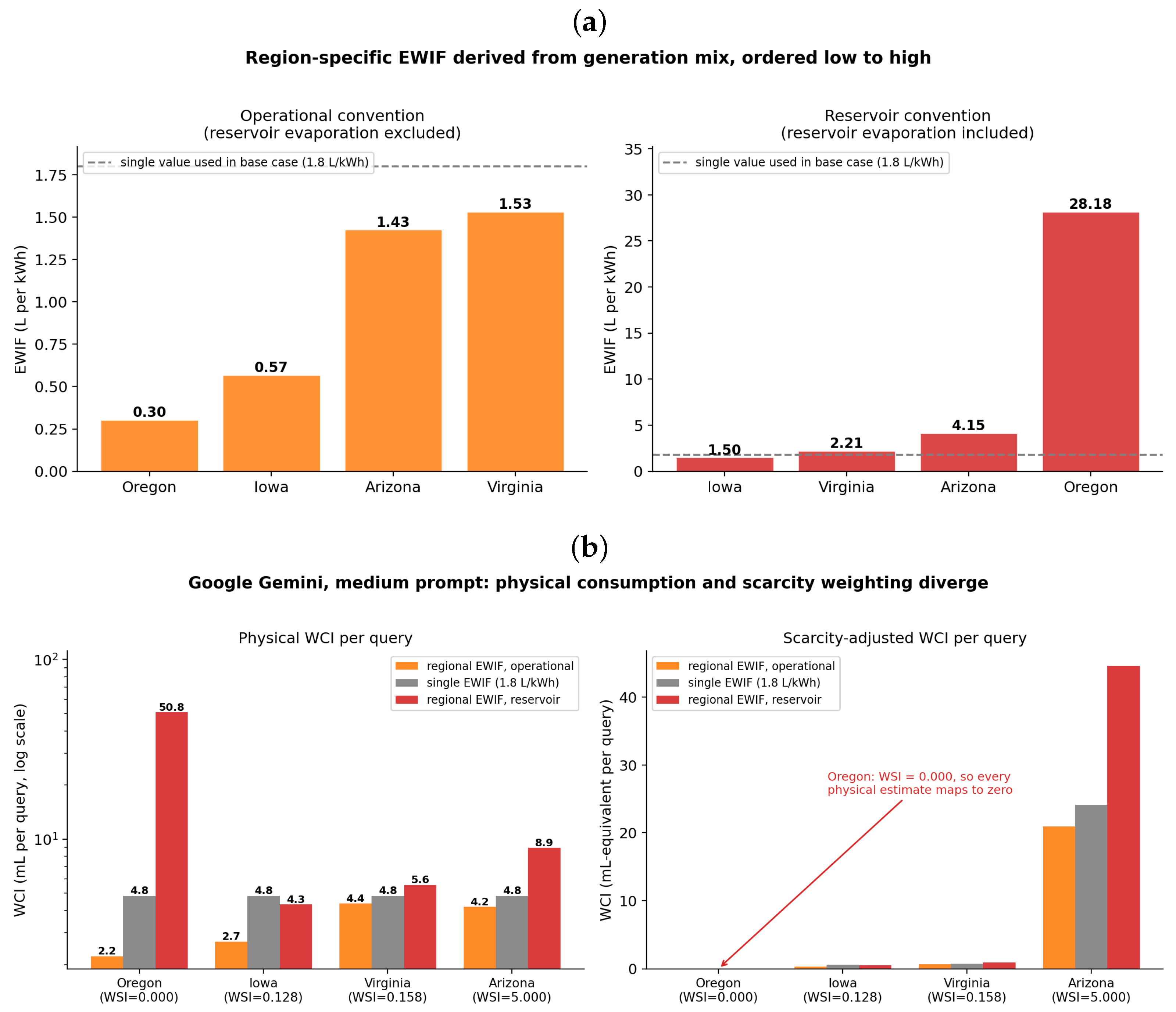
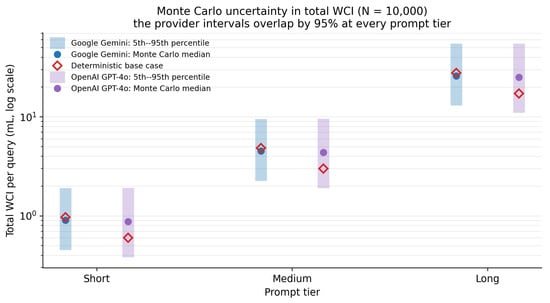
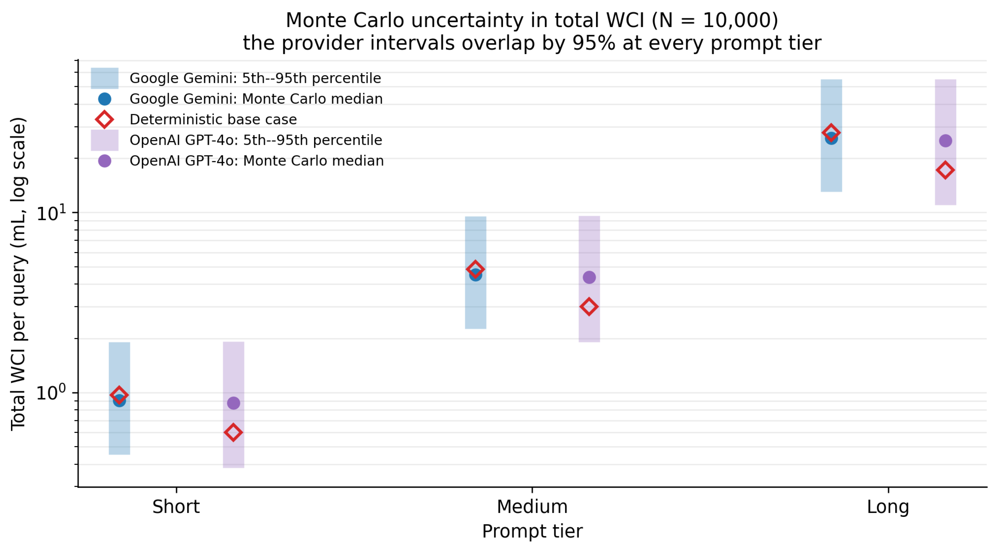
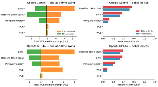
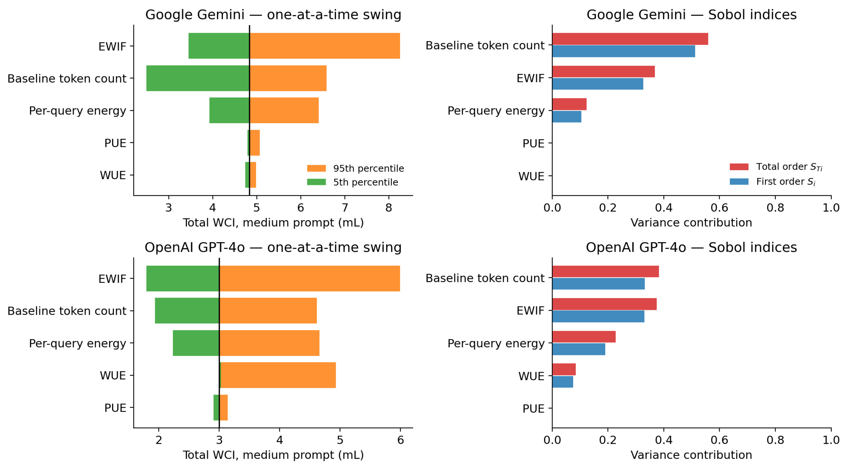

Disclaimer/Publisher’s Note: The statements, opinions and data contained in all publications are solely those of the individual author(s) and contributor(s) and not of MDPI and/or the editor(s). MDPI and/or the editor(s) disclaim responsibility for any injury to people or property resulting from any ideas, methods, instructions or products referred to in the content. |
© 2026 by the authors. Licensee MDPI, Basel, Switzerland. This article is an open access article distributed under the terms and conditions of the Creative Commons Attribution (CC BY) license.