Machine Learning Classification and Adaptive Power Control for RGB Underwater Visible Light Communication

Abstract

Underwater visible light communication (UVLC) offers high data rates over acoustic and radio-frequency links but is highly sensitive to bubble-induced scattering. This paper presents an RGB wavelength-division-multiplexed UVLC system simulated in OptiSystem across clear-water, intermediate, and bubble-induced turbidity conditions. Eye-diagram features are classified using XGBoost, achieving 98.75% test accuracy and 96.18% (±2.17%) repeated cross-validation accuracy, statistically validated against SVM and Random Forest. A held-out intermediate-turbidity set, unseen during training, is correctly identified by wavelength with 92.31–70.65% accuracy across 25–75% turbidity. An independently computed Mie scattering calculation shows bubble-induced scattering becomes wavelength-insensitive at realistic bubble sizes, consistent with the classifier’s confusion pattern. A systematic grid search over laser bias and modulation current on the blue channel identifies a distinct optimal operating point for clear-water and bubble-induced conditions, with bubble-induced BER reaching $6.95\times {10}^{-9}$ at its optimum, and indicates a sharp, condition-dependent transition in which settings tolerated under clear water drive the bubble-induced link toward its estimated reliability limit. Shannon capacity analysis indicates multi-gigabit-per-second headroom, and comparison with acoustic and radio-frequency alternatives confirms UVLC’s data-rate advantage at short range. The framework connects physical-layer simulation, classification, and characterized adaptive control within a single validated system.

1. Introduction

Underwater communication is essential for environmental monitoring, autonomous underwater vehicles (AUVs), and oceanographic data collection, but conventional technologies face significant physical limitations.

Acoustic communication supports data rates of tens of kilobits per second with high latency and multipath interference. Radio frequency (RF) communication in seawater is highly attenuated by water’s conductivity, limiting practical data rates to tens or hundreds of bits per second over short distances [1].

Underwater visible light communication (UVLC) offers a high-speed alternative, exploiting the wide optical spectrum to achieve data rates of several gigabits per second under controlled conditions [2], with low latency and high bandwidth [1]. Its performance is nonetheless highly sensitive to absorption, scattering, turbulence, and bubble-induced distortions, which degrade signal quality and limit range in dynamic underwater environments [3].

Eye diagram analysis is an established tool for evaluating optical signal integrity, providing eye opening, jitter, and signal-to-noise ratio (SNR) as indicators of channel condition. Coupling these metrics with machine learning-based classification offers a route to automated channel assessment.

Underwater optical wireless communication (UOWC) has been surveyed extensively as an alternative to acoustic and RF links, offering higher data rates and lower latency at the cost of a strongly attenuating channel [4,5], establishing the core taxonomy of absorption, scattering, and turbulence impairments this work builds upon. Theocharidis and Kavallieratou [1] reviewed underwater communication technologies spanning acoustic, RF, and optical approaches.

RGB laser-based WDM has driven recent throughput gains. Zhang et al. [2] demonstrated a dense blue–green WDM system exceeding 10 Gbit/s under turbidity-tolerant conditions. Janarthanan and Gauni [6] proposed a 32-channel dense WDM system supporting 320 Gbps over 200–350 m. Rehman et al. [3] examined adaptive UVLC operation, motivating the channel-aware approach pursued here.

Abd El-Mottaleb et al. proposed two OCDMA-based approaches for secure, high-data-rate UOWC: an IRSM-OCDMA framework for secure RGB image transmission at up to 30 Gbps [7], and a related green-spectrum (532–538 nm) system reporting Q-factor and BER over distances up to 50 m [8], providing a benchmark directly comparable to the results in Section 3.1.

NRZ-OOK is favored for its simple, direct mapping between bit value and optical intensity. Dong et al. [9] demonstrated 1 Gbps at 450 nm over 250 m using equalization, the first Gbps-class UWOC demonstration beyond 250 m. The modulation scheme used here follows this same principle (Section 2.1).

Chaudhary [10] demonstrated polarization-multiplexed MIMO mitigating salinity-induced degradation. Ramley et al. [11] reviewed Monte Carlo methods for underwater radiative transfer. Vali et al. [12] surveyed turbulence characterization in UOWC, typically treated independently of the absorption/scattering attenuation modeled here.

Bubble-induced scattering has been characterized since Davis’s analysis of light scattering by an air bubble in water [13], establishing that bubbles larger than the incident wavelength scatter in the Mie/geometric-optics regime rather than the wavelength-selective Rayleigh regime (Section 2.10).

Machine learning applications to VLC channel estimation, noise mitigation, and symbol detection have grown rapidly [14]. Zhao et al. [15] proposed a recurrent network for underwater link adaptation from raw waveforms, without re-simulated validation of the resulting adaptation. Salama and Aly [16] combined deep learning models for OFDM channel estimation. Skoog et al. [17] applied SVM to fiber-optic eye diagrams for impairment identification, without connecting the classifier to transmitter control. Islam et al. [18] applied XGBoost to FSO turbulence prediction with over 98% accuracy, closely related methodologically but addressing atmospheric turbulence rather than underwater scattering.

Existing work largely treats these problems separately: physical-layer characterization, channel classification, and adaptive control are rarely combined and verified together, and adaptive-control proposals typically demonstrate a single operating point rather than characterizing how the optimal transmitter configuration itself depends on channel condition. This paper couples eye-diagram classification to an independently computed physical explanation of the classifier’s behavior, and to a systematic grid search over transmitter parameters that quantifies, rather than assumes, how the optimal operating point and the boundary of link failure shift between channel conditions.

The paper is organized as follows. Section 2.1 describes the RGB WDM system and underwater channel model. Section 2.3, Section 2.4 and Section 2.5 describe the eye-diagram feature extraction and classification methodology. Section 2.7, Section 2.8, Section 2.9 and Section 2.10 describe the adaptive power strategy, the parameter sweep methodology, the turbidity gradient, and the Mie scattering computation. Section 3 reports physical-layer, sweep, classification, and generalization results, followed by Section 4 and Section 5.

2. Materials and Methods

2.1. System Model

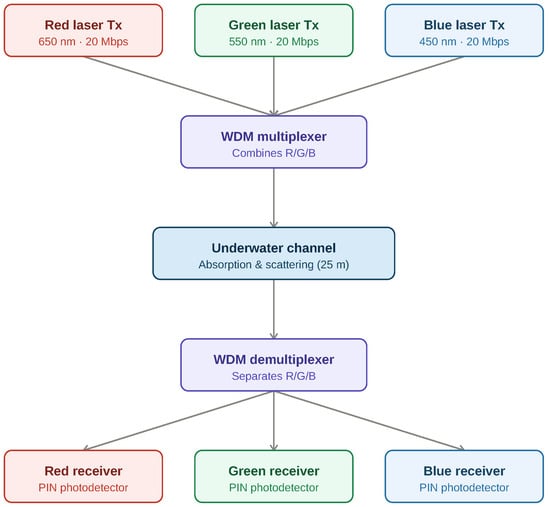
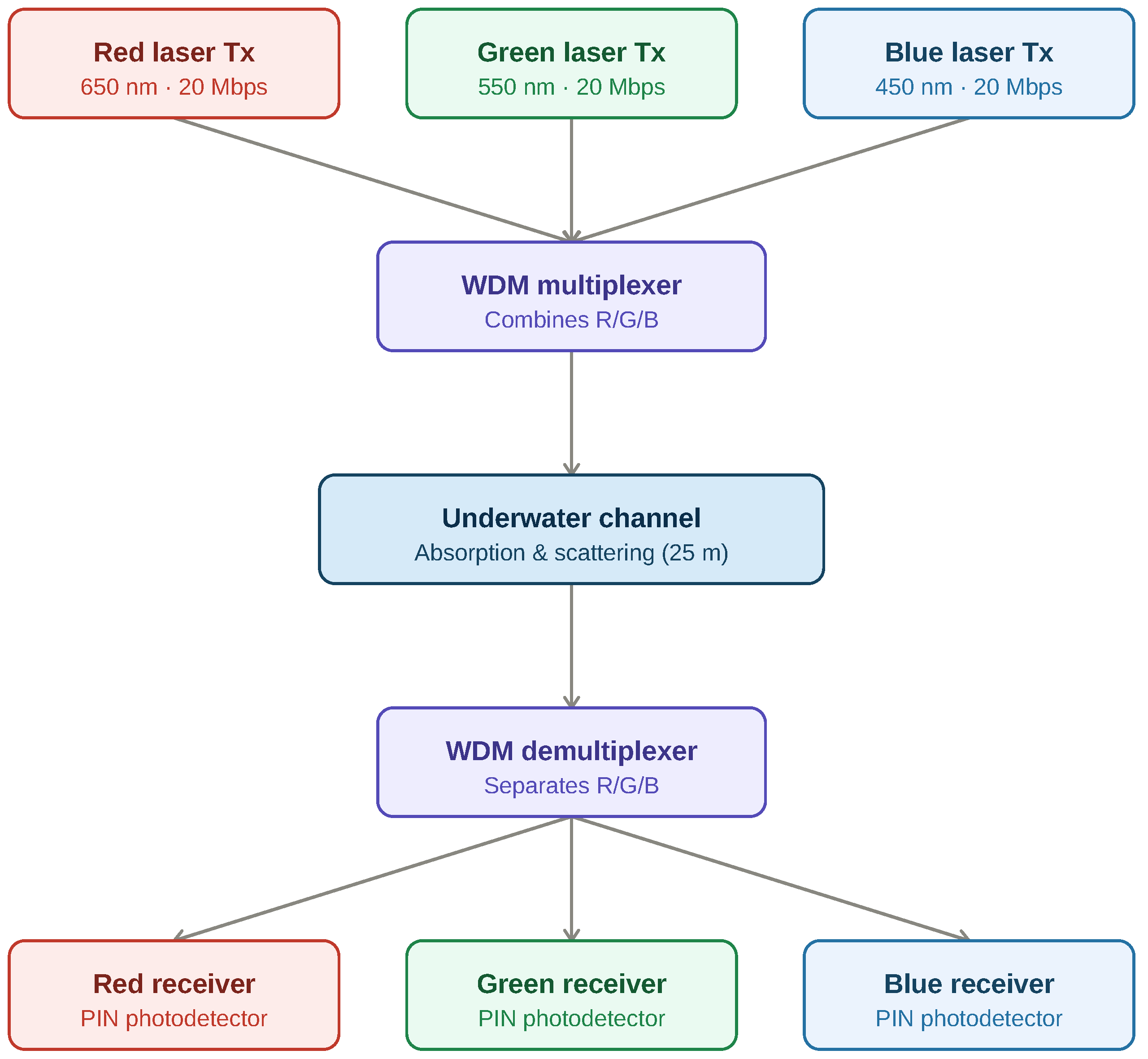
The proposed UVLC system is designed and simulated in OptiSystem; its architecture is shown in Figure 1. Wavelength division multiplexing (WDM) transmits red, green, and blue (450/550/650 nm) laser signals simultaneously over a shared underwater channel. This RGB convention follows standard practice in the VLC literature [4,5]: the three wavelengths span the visible spectrum with roughly equal spacing, maximizing WDM channel separation, and RGB sources are widely available and compatible with combined illumination and communication [2,6].

Figure 1. RGB WDM UVLC system architecture.

Three sources are modulated using Non-Return-to-Zero On-Off Keying (NRZ-OOK) and combined by a WDM multiplexer before transmission through the underwater channel. Table 1 lists the key parameters.

Table 1. Key simulation parameters.

Parameter	Value
Wavelengths (R/G/B)	650/550/450 nm
Data rate per channel	20 Mbps
Modulation	NRZ-OOK
Laser threshold current (R/G/B)	33.46 mA (all channels)
Laser threshold power (R/G/B)	0.037/0.044/0.054 mW
Link distance	25 m
Absorption coeff. (clear/bubble)	0.0405/0.180 m−1
Scattering coeff. (clear/bubble)	0.0025/0.219 m−1
Photodetector sensitivity	10 A/W

Modulation Scheme

The NRZ-OOK transmitted signal is

$$P\left(t\right)=\sum _k{b}_{k}p(t-k{T}_b),b_k\in \{0,1\},$$

(1)

where $b_k$ is the k-th bit, $p\left(t\right)$ the rectangular pulse over one bit period, and $T_b$ the bit period for the 20 Mbps rate. Optical power switches between a low (“space,” $P_0$) and high (“mark,” $P_1$) level, with extinction ratio $\mathrm{ER}=P_1/P_0$ governing eye opening, Q-factor, and BER (Section 3).

Clear-water and bubble-induced conditions are represented by the coefficient pairs in Table 1, consistent with commonly used underwater channel models [11]. Attenuation follows the Beer–Lambert law [19]:

$$P_r=P_t{e}^{-cd},$$

(2)

where $P_t$ is transmitted power, $P_r$ received power, c the attenuation coefficient, and d the propagation distance. At the receiver, a WDM demultiplexer separates the channels for detection; thermal and shot noise are included in the receiver model.

2.2. Eye Diagram Dataset

Eye diagrams are generated in OptiSystem’s Eye Diagram Analyzer for each channel-condition combination, with the amplitude axis shared across the three wavelengths within each condition type (clear or bubble-induced). Images are resized to 128 × 128 pixels and converted to grayscale.

The dataset spans six classes, blue, green, and red, each under clear and bubble-induced conditions, with 50 original images per class (300 total). Data augmentation (horizontal flip, ±5° rotation, additive Gaussian noise) expands this to 1200 images. Q-factor, minimum BER, and eye height are also recorded directly from the Eye Diagram Analyzer for each condition.

2.3. Feature Extraction

Eleven features are extracted per eye diagram. For pixel intensities $x_1,\dots ,x_N$:

$$\begin{array}{cc}\hfill \mathrm{Mean}:& \mu ={\displaystyle \frac{1}{N}}{\displaystyle \sum _{i=1}^N}{x}_i\hfill \end{array}$$

(3)

$$\begin{array}{cc}\hfill \mathrm{Standard}\mathrm{deviation}:& \sigma =\sqrt{{\displaystyle \frac{1}{N}}\sum _{i=1}^N{(x_i-\mu )}^2}\hfill \end{array}$$

(4)

$$\begin{array}{cc}\hfill \mathrm{Skewness}:& {\gamma }_1={\displaystyle \frac{\frac{1}{N}{\sum }_{i=1}^N{(x_i-\mu )}^3}{{\sigma }^3}}\hfill \end{array}$$

(5)

$$\begin{array}{cc}\hfill \mathrm{Excess}\mathrm{kurtosis}:& {\gamma }_2={\displaystyle \frac{\frac{1}{N}{\sum }_{i=1}^N{(x_i-\mu )}^4}{{\sigma }^4}}-3\hfill \end{array}$$

(6)

$$\begin{array}{cc}\hfill \mathrm{Interquartile}\mathrm{range}:& \mathrm{IQR}=Q_3-Q_1,\hfill \end{array}$$

(7)

plus median, edge density (Canny detector), average FFT magnitude, and eye opening, jitter, and SNR:

$${\mathrm{SNR}}_{\mathrm{dB}}=10{log}_{10}\left({\displaystyle \frac{P_{\mathrm{signal}}}{P_{\mathrm{noise}}}}\right).$$

(8)

This image-derived SNR is distinct from the electrical SNR reported in Section 3.1, derived analytically from Q-factor (Section 2.11).

2.4. Model Training

The dataset is split 80/20 using a stratified, group-aware scheme: all augmented variants of a source image stay in the same partition, and each class contributes equally to the test set, preventing leakage between augmented copies.

Features are standardized by z-score, fit on the training partition only:

$$z_i={\displaystyle \frac{x_i-{\mu }_{\mathrm{train}}}{{\sigma }_{\mathrm{train}}}}.$$

(9)

Tree-based models such as XGBoost are largely insensitive to feature scale, but standardization is applied uniformly across all three classifiers compared here for consistent preprocessing and to avoid disadvantaging the scale-sensitive SVM classifier.

An XGBoost classifier with 300 estimators, max depth 6, learning rate 0.1, subsample 0.8 is compared against SVM (RBF kernel) and Random Forest on identical splits, alongside a hyperparameter search, a full feature ablation, and a hierarchical condition-then-wavelength classifier.

2.5. Model Evaluation

Performance is evaluated via accuracy, precision, recall, F1-score, and confusion matrix. Stratified group-aware 5-fold cross-validation is repeated across five fold assignments (25 folds total); both the single-fold and repeated-fold results are reported (Section 3.7), with the repeated scheme as the primary metric given its lower variance. A paired t-test across the 25 folds compares classifier architectures.

2.6. Adaptive Power Strategy

When bubble-induced conditions are classified, the transmitter’s bias current and modulation peak current are adjusted, since these are the parameters OptiSystem exposes as independently controllable and that determine extinction ratio (Equation (1)). Clear-water conditions retain nominal parameters, subject to the refinement described in Section 2.8.

2.7. Adaptive Power Validation Procedure

An initial adjustment (bias 35 mA, modulation 55 mA) was derived from the extinction-ratio argument in Section 2.6, positioning bias current near the measured laser threshold (33.46 mA) while widening modulation swing, following a small number of manual trials; an earlier 42/42 mA trial underperformed the 40/40 mA baseline (Q-factor 4.805 vs. 5.08), motivating the shift toward threshold-proximate bias.

When bias current sits well above threshold, the “space” level itself lases at significant power, compressing mark/space contrast regardless of modulation swing. Positioning bias near threshold instead keeps the space level near turn-on, while a wide swing drives the mark level into the linear lasing region, maximizing $\mathrm{ER}=P_1/P_0$, eye opening, Q-factor, and BER. This 35/55 mA configuration was re-simulated under bubble-induced conditions for all three channels (Section 3) and served as the starting point for the systematic search described next.

2.8. Parameter Sweep Methodology

To characterize the transmitter parameter space beyond the single point validated above, a full grid search was performed over bias current (34–40 mA, 1 mA steps) and modulation current (40–100 mA, 10 mA steps), evaluated separately under clear-water and bubble-induced conditions. The bias range was bounded below by the laser threshold current (33.46 mA) and above by the original 40 mA baseline; the modulation range extended from the baseline to 100 mA, confirmed via the laser’s measured L-I characteristic to remain within its linear operating region across this full range, with no evidence of saturation.

The sweep was performed on the blue channel as an initial characterization. All three RGB lasers share an identical threshold current in the OptiSystem model, and this shared threshold was the basis for applying the single-point validation in Section 2.7 uniformly across channels. Threshold current is not the same quantity as slope efficiency, however, and the three lasers exhibit different threshold powers (Table 1), which indicates their slope efficiencies also differ. Because of this difference, the specific bias/modulation combination found to be optimal for blue is not assumed to also be optimal for green and red. Whether the same qualitative pattern observed for blue, particularly the condition-dependent failure boundary, also occurs for green and red has not yet been tested, and confirming this is identified as a priority extension in Section 4.4.

Q-factor and BER were recorded from the Eye Diagram Analyzer at each of the 98 resulting combinations. A single fixed bit sequence (Section 2.2) was used across all 49 combinations per condition to isolate the effect of the parameter change from run-to-run bit-pattern variation; each grid point therefore reflects one deterministic realization, and the implications of this for the sweep’s statistical robustness are discussed in Section 4.4.

The average electrical drive current for NRZ-OOK modulation, assuming equal-probability bits, is $I_{\mathrm{avg}}=I_{\mathrm{bias}}+0.5I_{\mathrm{mod}}$. This value is used in Section 4.4 to compare the electrical cost of any recommended operating point against the original 40/40 mA baseline, which corresponds to an average drive current of 60 mA.

2.9. Turbidity Gradient and Generalization

Three intermediate turbidity levels (25%, 50%, 75%) were constructed by linearly interpolating absorption and scattering coefficients between the clear and bubble-induced endpoints (Table 1). These percentages denote the fractional position between the clear-water and bubble-induced coefficient values. The resulting five-point gradient was simulated for all three channels using the same configuration as Section 2.1.

Eye diagram images were also captured at each intermediate level. For each, 60% of source images were added to training as new labeled classes, and the remaining 40% held out entirely until final evaluation, testing whether the classifier extends beyond the two extreme conditions it was originally trained on.

2.10. Mie Scattering Computation

Mie scattering efficiency was computed independently of OptiSystem using the miepython Python package (version 3.3.0). Following Davis [13], the relative refractive index of an air bubble in water is

$$m={\displaystyle \frac{n_{\mathrm{air}}}{n_{\mathrm{water}}}}={\displaystyle \frac{1.0003}{1.33}}\approx 0.752,$$

(10)

and the size parameter [13] is

$$x={\displaystyle \frac{\pi d}{{\lambda }_{\mathrm{medium}}}},{\lambda }_{\mathrm{medium}}={\displaystyle \frac{{\lambda }_{\mathrm{vacuum}}}{n_{\mathrm{water}}}},$$

(11)

with $d=2a$ the bubble diameter. Scattering efficiency $Q_{sca}$ follows the standard Mie solution [13], computed for the three RGB wavelengths across bubble radii of 1–1000 $\mathsf{\mu }$m.

2.11. Shannon Capacity Calculation

Theoretical capacity was computed via the Shannon–Hartley theorem [20]:

$$C=B{log}_2(1+\mathrm{SNR}),$$

(12)

with B the measured $-3$ dB bandwidth (Table 2) and SNR derived from Q-factor [21]:

$${\mathrm{SNR}}_{\mathrm{dB}}=20{log}_{10}\left(Q\right).$$

(13)

Table 2. Measured bandwidth.

Laser Color	Bandwidth (GHz)
Blue (450 nm)	0.82
Green (550 nm)	0.60
Red (650 nm)	0.48
Total Bandwidth	1.90

3. Results

3.1. Eye Diagrams and Bandwidth

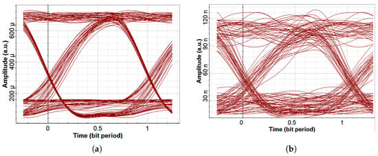
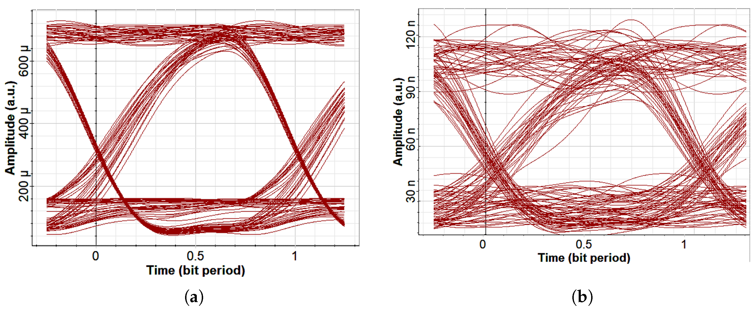
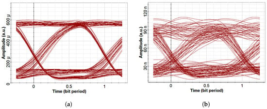
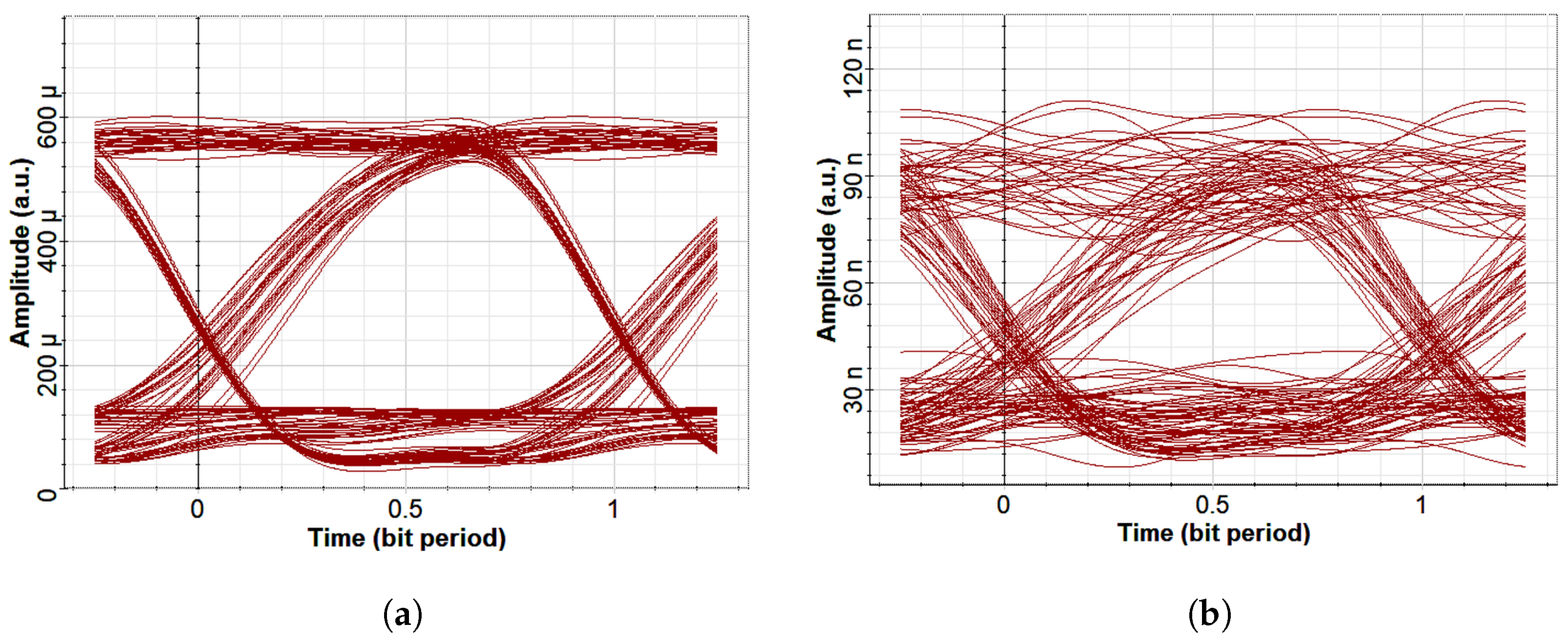
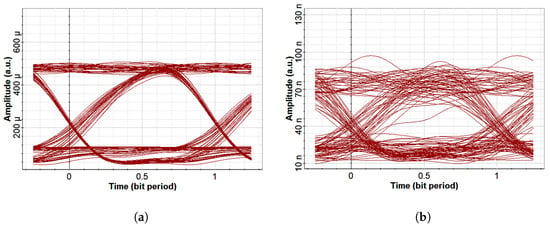
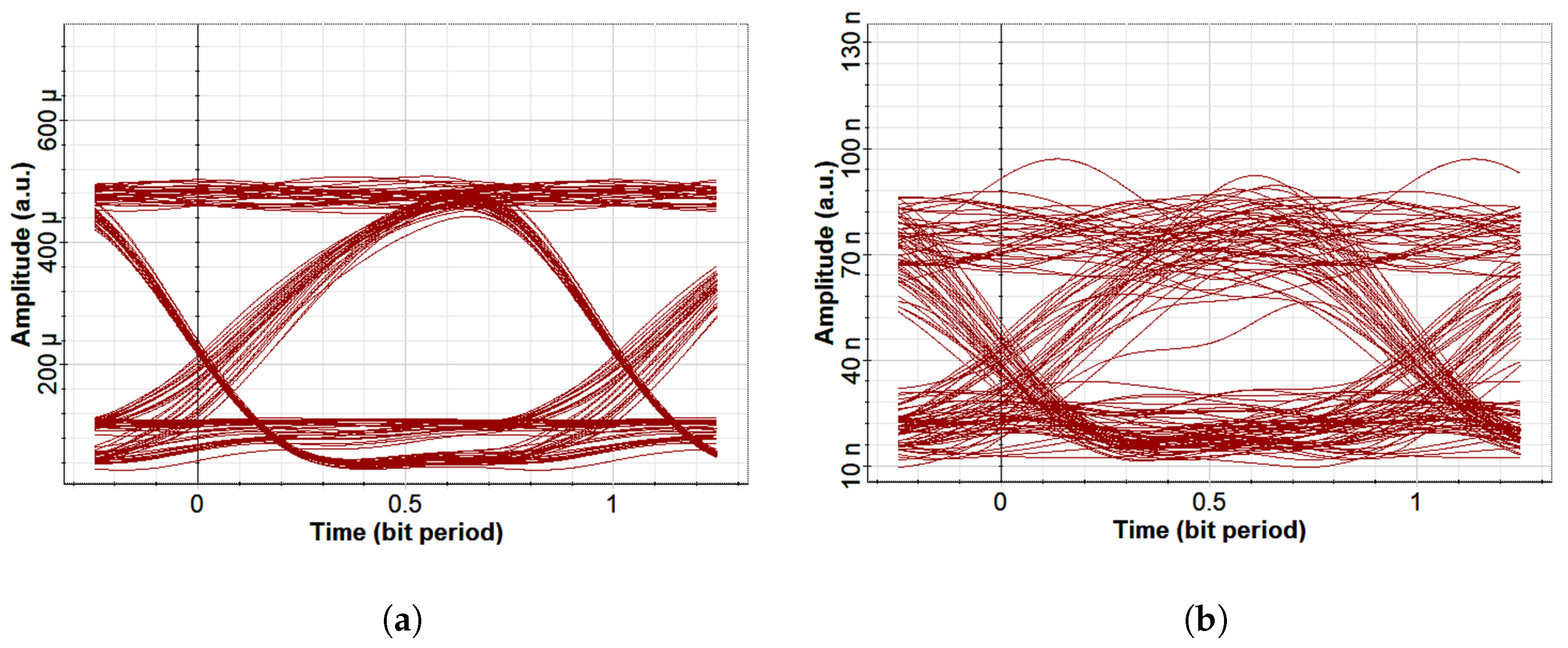
Figure 2, Figure 3 and Figure 4 show measured eye diagrams for each channel under clear and bubble-induced conditions.

Figure 2. Blue channel: (a) clear, (b) bubble-induced. Amplitude axes are shared across all three colors within each condition type (clear and bubble-induced use separate ranges, since received power differs by about three orders of magnitude between them).

Figure 3. Green channel: (a) clear, (b) bubble-induced. Amplitude axes are shared across all three colors within each condition type (clear and bubble-induced use separate ranges, since received power differs by about three orders of magnitude between them).

Figure 4. Red channel: (a) clear, (b) bubble-induced. Amplitude axes are shared across all three colors within each condition type (clear and bubble-induced use separate ranges, since received power differs by about three orders of magnitude between them).

Blue shows the largest eye opening under both conditions, followed by green and red, consistent with lower absorption at shorter wavelengths. Bubble-induced scattering degrades all channels, most severely for red.

Table 2 gives measured $-3$ dB bandwidth per channel.

Bandwidth exceeds the 20 Mbps signal bandwidth substantially, indicating headroom for higher-rate operation; WDM gives a total system bandwidth of approximately 1.90 GHz.

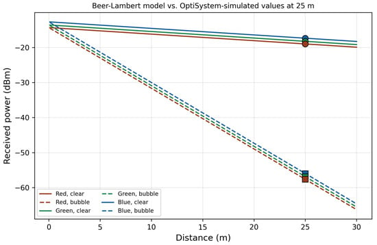
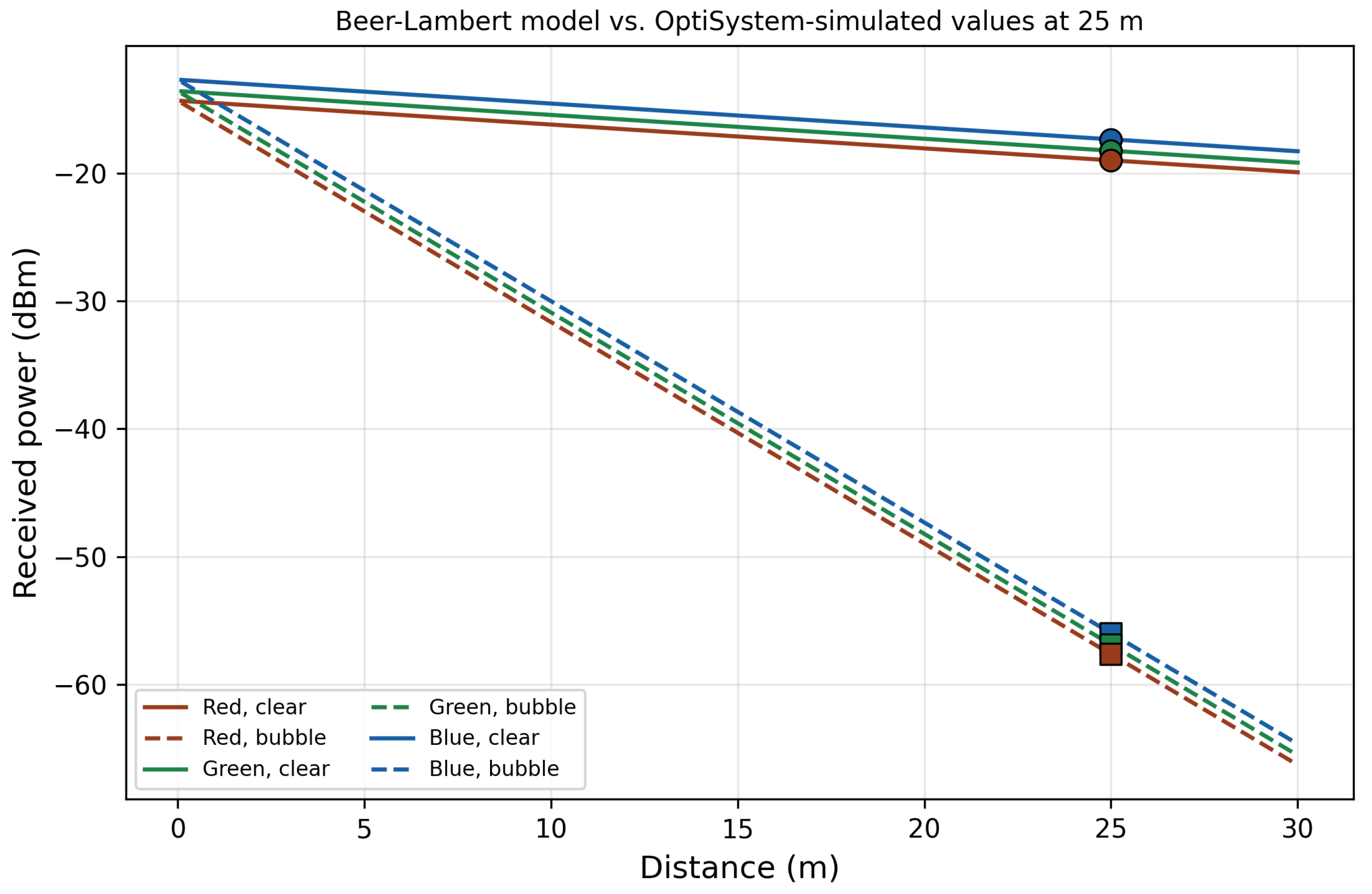
Received power at 25 m (Equation (2)) is 12.6, 15.0, and 18.4 $\mathsf{\mu }$W for red, green, and blue under clear water, dropping to 1.72, 2.05, and 2.51 nW under bubble-induced conditions, roughly 39 dB of additional loss. Figure 5 shows this trend with distance.

Figure 5. Received power vs. distance (Equation (2)); markers show the 25 m values from Table 3.

Table 3 summarizes Q-factor, BER, eye height, received power, and SNR for all six conditions.

Table 3. Communication performance metrics.

Condition	Q-Factor	BER	Rx Power	Eye Height	SNR (dB)
Blue-Clear	10.27	$4.36\times {10}^{-25}$	18.4 $\mathsf{\mu }$W	$4.09\times {10}^{-4}$	20.23
Blue-Bubble	5.08	$1.92\times {10}^{-7}$	2.51 nW	$3.22\times {10}^{-8}$	14.12
Green-Clear	9.67	$1.91\times {10}^{-22}$	15.0 $\mathsf{\mu }$W	$3.23\times {10}^{-4}$	19.71
Green-Bubble	4.48	$3.66\times {10}^{-6}$	2.05 nW	$2.17\times {10}^{-8}$	13.03
Red-Clear	9.37	$3.44\times {10}^{-21}$	12.6 $\mathsf{\mu }$W	$2.70\times {10}^{-4}$	19.43
Red-Bubble	4.31	$7.92\times {10}^{-6}$	1.72 nW	$1.69\times {10}^{-8}$	12.69

Blue leads in Q-factor and BER under both conditions; ordering is monotonic (blue > green > red) throughout. Under bubble-induced conditions, green and red are closest in Q-factor (4.48 vs. 4.31) and BER, while blue remains distinct (5.08, $1.92\times {10}^{-7}$).

3.2. Turbidity Gradient

Table 4 and Figure 6 give Q-factor, BER, eye height, and SNR across the full gradient.

Table 4. Physical-layer metrics across the turbidity gradient (fractional interpolation, not NTU).

Turbidity	Channel	Q-Factor	BER	Eye Height	SNR (dB)
0% (Clear)	Blue	10.27	$4.36\times {10}^{-25}$	$4.09\times {10}^{-4}$	20.23
	Green	9.67	$1.91\times {10}^{-22}$	$3.23\times {10}^{-4}$	19.71
	Red	9.37	$3.44\times {10}^{-21}$	$2.70\times {10}^{-4}$	19.43
25%	Blue	9.665	$1.962\times {10}^{-22}$	$4.290\times {10}^{-5}$	19.70
	Green	9.529	$7.346\times {10}^{-22}$	$3.469\times {10}^{-5}$	19.58
	Red	9.363	$3.717\times {10}^{-21}$	$2.902\times {10}^{-5}$	19.43
50%	Blue	9.532	$7.306\times {10}^{-22}$	$4.595\times {10}^{-6}$	19.58
	Green	9.417	$2.173\times {10}^{-21}$	$3.732\times {10}^{-6}$	19.48
	Red	9.219	$1.409\times {10}^{-20}$	$3.119\times {10}^{-6}$	19.30
75%	Blue	9.471	$1.311\times {10}^{-21}$	$4.539\times {10}^{-6}$	19.53
	Green	9.239	$1.174\times {10}^{-20}$	$3.688\times {10}^{-6}$	19.31
	Red	9.110	$3.988\times {10}^{-20}$	$3.089\times {10}^{-6}$	19.19
100% (Bubble)	Blue	5.08	$1.92\times {10}^{-7}$	$3.22\times {10}^{-8}$	14.12
	Green	4.48	$3.66\times {10}^{-6}$	$2.17\times {10}^{-8}$	13.03
	Red	4.31	$7.92\times {10}^{-6}$	$1.69\times {10}^{-8}$	12.69

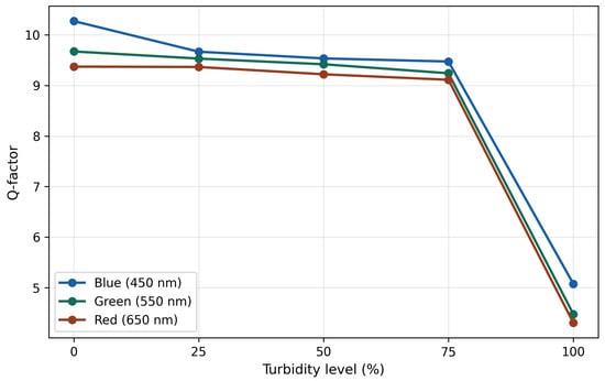
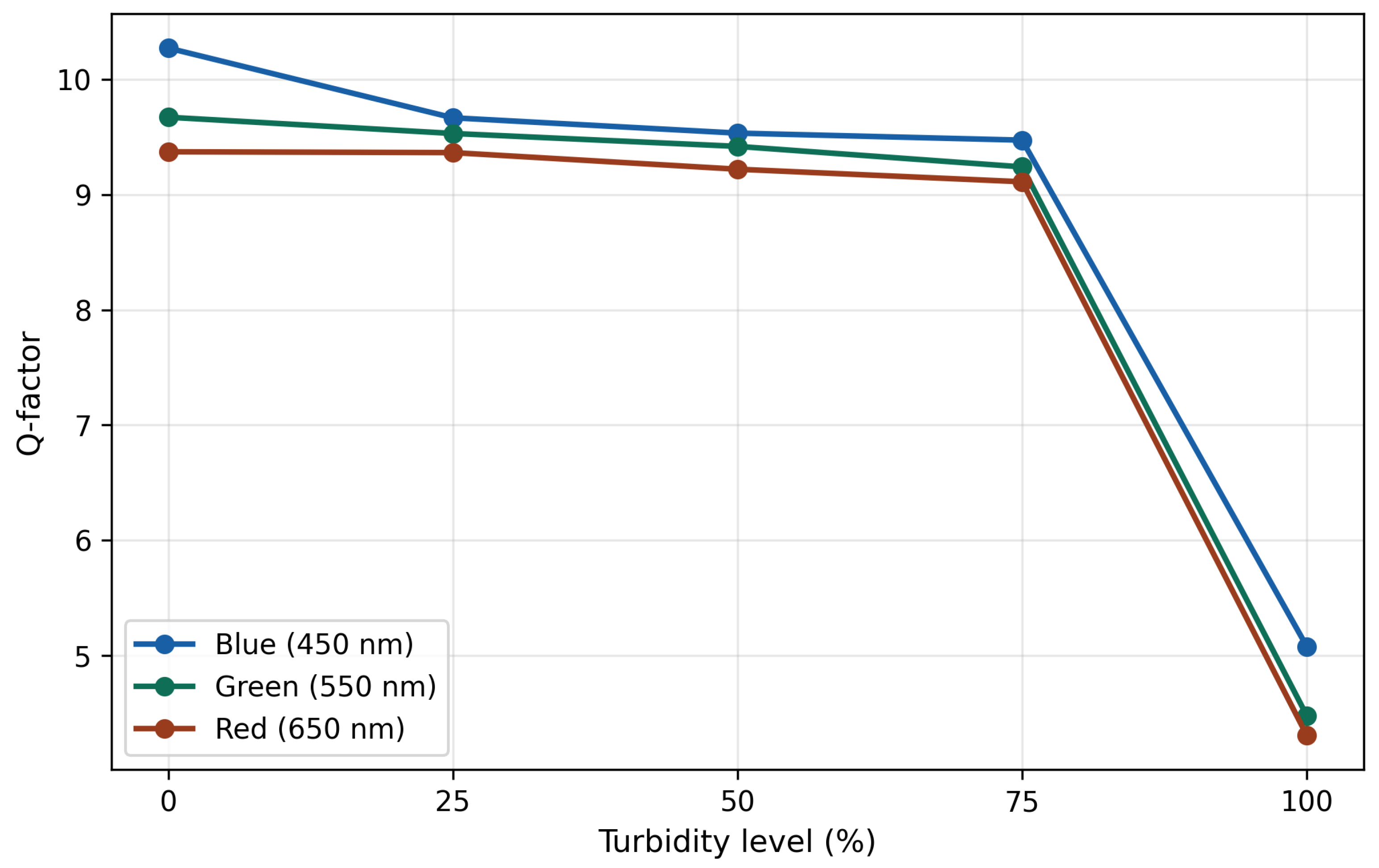
Figure 6. Q-factor vs. turbidity level.

Q-factor declines gradually through 75% turbidity (blue: 10.27 to 9.471, 7.8%), then collapses sharply toward the bubble endpoint (9.471 to 5.08, 46%), with BER worsening by 13–14 orders of magnitude over that final step.

3.3. Mie Scattering and Classification Confusion

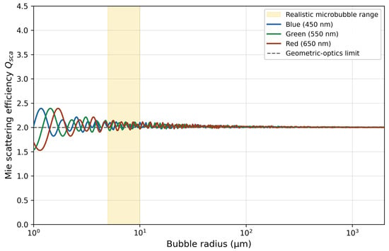
Figure 7 shows computed $Q_{sca}$ for the three wavelengths across 1–1000 $\mathsf{\mu }$m.

Figure 7. Mie scattering efficiency vs. bubble radius, converging to $Q_{sca}\to 2$ beyond ∼10 $\mathsf{\mu }$m; shaded region marks realistic microbubble sizes.

Below ∼2 $\mathsf{\mu }$m, scattering is wavelength-dependent (up to 27.6% difference between blue and green at 1 $\mathsf{\mu }$m). Beyond 5–10 $\mathsf{\mu }$m, all three converge to $Q_{sca}\approx 2$, within 1–2% of each other, with no single pair consistently closest.

This matches the classifier’s behavior: at full bubble-induced turbidity, its dominant confusion is between green and red, matching their closest Q-factor and BER values (Table 3). At intermediate turbidity (Section 3.8), the dominant confusion instead shifts to green–blue and red–green, while blue–red, the most physically dissimilar pair, stays rare throughout. As the scattering regime evolves across the gradient, the specific pair the classifier confuses shifts with it, while the underlying pattern, physically similar channels being harder to separate, holds at every level.

3.4. Shannon Capacity

Table 5 gives theoretical capacity for all six conditions.

Table 5. Theoretical Shannon capacity.

Condition	SNR (Linear)	Capacity (Gbps)
Blue-Clear	105.4	5.52
Blue-Bubble	25.8	3.89
Green-Clear	93.6	3.94
Green-Bubble	20.1	2.64
Red-Clear	87.7	3.11
Red-Bubble	18.6	2.06

Capacity stays in the multi-gigabit range even under bubble-induced degradation, over two orders of magnitude above the 20 Mbps rate simulated here.

3.5. Adaptive Power Validation

Table 6 gives Q-factor, BER, eye height, and SNR before and after the initial current adjustment (Section 2.7) under bubble-induced conditions.

Table 6. Bubble-induced conditions before and after initial laser current adjustment (35/55 mA).

Condition	Q-Factor		BER		Eye Height		SNR (dB)
	Before	After	Before	After	Before	After	Before	After
Blue-Bubble	5.08	7.959	$1.92\times {10}^{-7}$	$8.40\times {10}^{-16}$	$3.22\times {10}^{-8}$	$5.49\times {10}^{-8}$	14.12	18.02
Green-Bubble	4.48	7.247	$3.66\times {10}^{-6}$	$1.99\times {10}^{-13}$	$2.17\times {10}^{-8}$	$4.23\times {10}^{-8}$	13.03	17.20
Red-Bubble	4.31	6.093	$7.92\times {10}^{-6}$	$5.22\times {10}^{-10}$	$1.69\times {10}^{-8}$	$2.95\times {10}^{-8}$	12.69	15.70

BER improves by 9, 7, and 4 orders of magnitude for blue, green, and red at this single validated point.

3.6. Parameter Sweep Results

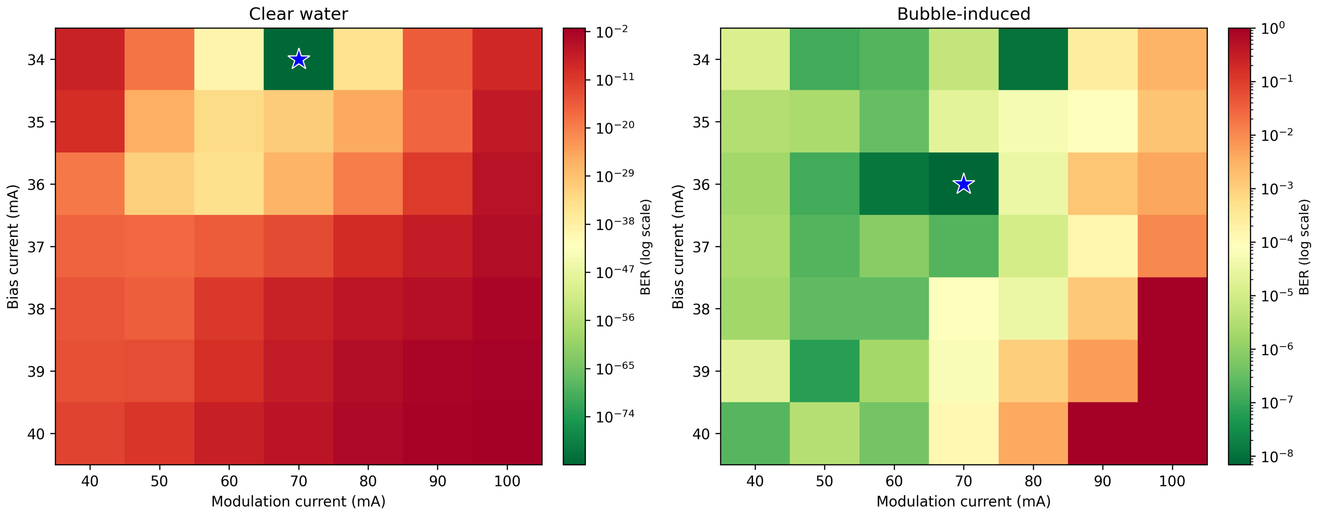
Figure 8 shows the complete 49-point BER grid for the blue channel under clear-water and bubble-induced conditions, from the sweep described in Section 2.8.

Figure 8. BER across the bias/modulation current grid, blue channel, clear water and bubble-induced conditions (star marks each panel’s minimum).

Table 7 summarizes the optimal point and the most severe failure observed in each condition.

Table 7. Sweep results: optimal and worst-case BER by condition (blue channel).

	Clear Water	Bubble-Induced
Optimal (Bias, Modulation)	34 mA, 70 mA	36 mA, 70 mA
Optimal BER	$1.01\times {10}^{-83}$	$6.95\times {10}^{-9}$
Worst BER observed	$4.69\times {10}^{-2}$	$1.0$

The clear-water optimal BER value is extremely small and lies at the outer limit of what the estimator can meaningfully resolve; it should therefore be read simply as “effectively error-free” rather than as a precise, literal number. The bubble-induced worst-case value of 1.0 represents the estimator’s reported reliability limit under the most severe tested settings. The optimal bias current differs between conditions: 34 mA for clear water, 36 mA under bubble-induced scattering. Both conditions share the same optimal modulation current (70 mA), but diverge sharply away from their respective optima. Clear water degrades gracefully across the tested grid, reaching a worst-case BER of $4.69\times {10}^{-2}$ at the extreme corner (40/100 mA), degraded, but not failed. Bubble-induced conditions instead report BER exactly equal to 1.0 at five grid points (38/100, 39/90, 39/100, 40/90, 40/100 mA). A reported BER of exactly 1.0 is consistent with complete eye closure, but can also reflect the Q-factor-based estimator saturating once the mark and space distributions fully overlap.

3.7. Classification Results

XGBoost achieves 98.75% test accuracy (Table 8; 240 samples, 60 unique source images). The per-class support counts in Table 8 are not uniformly 40, despite each of the six classes originally containing 50 source images. This arises from the group-aware stratified splitting procedure (Section 2.4): because all four samples belonging to one source image, the original plus three augmented variants, must remain together in the same partition, the split allocates whole groups of four samples to the test set rather than individual samples. Achieving both exact group integrity and exactly equal per-class proportions in a single split is not always possible, so individual classes receive 9, 10, or 11 source-image groups (36, 40, or 44 samples) in the test partition rather than exactly 10 each, while overall class balance remains approximately preserved. This is a documented property of group-constrained stratified splitting rather than a data preparation inconsistency, and the same procedure is applied consistently across all cross-validation folds reported in this study.

Table 8. XGBoost classification performance.

Class	Precision	Recall	F1-Score	Support
Bubble-Blue	1.00	1.00	1.00	44
Bubble-Green	0.95	0.97	0.96	40
Bubble-Red	0.97	0.95	0.96	40
Pure-Blue	1.00	1.00	1.00	36
Pure-Green	1.00	1.00	1.00	40
Pure-Red	1.00	1.00	1.00	40
Macro Avg	0.99	0.99	0.99	240
Weighted Avg	0.99	0.99	0.99	240

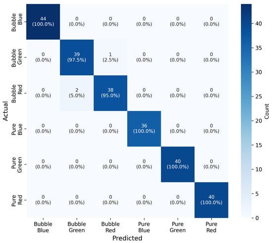
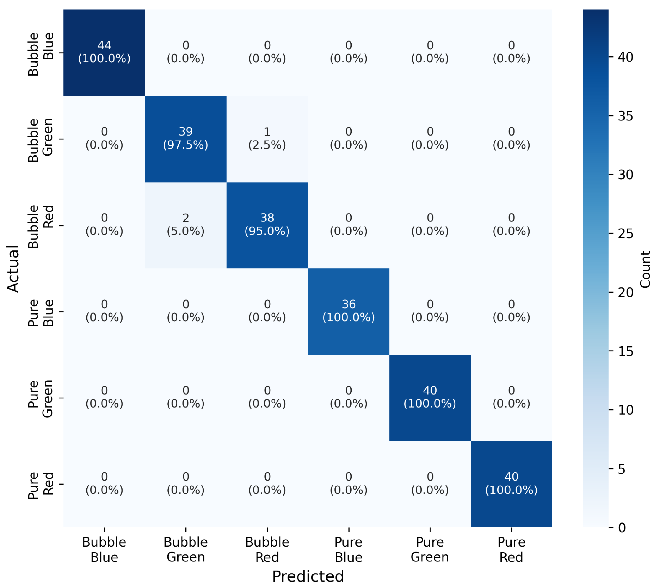
The confusion matrix (Figure 9) shows pure-water classes separate perfectly; all errors are confined to bubble-induced classes, dominated by mutual green–red confusion (1/40 green misclassified red, 2/40 red misclassified green), while bubble-induced blue is perfect (44/44).

Figure 9. Confusion matrix.

Single 5-fold cross-validation gives 97.50% (±1.69); repeated over 25 folds gives 96.18% (±2.17), adopted as the primary metric for its lower variance. Table 9 compares classifiers under both schemes.

Table 9. Classifier comparison, two validation schemes.

Classifier	Test Accuracy	Single 5-Fold CV	Repeated 5 × 5-Fold CV
XGBoost	98.75%	97.50% (±1.69)	96.18% (±2.17)
SVM (RBF kernel)	97.92%	96.50% (±1.93)	96.90% (±2.35)
Random Forest	98.33%	97.00% (±1.74)	96.40% (±2.26)

A paired t-test over the 25 repeated folds shows XGBoost (96.18%) differs significantly from SVM (96.90%; $t=-2.670$, $p=0.013$), but not from Random Forest (96.40%; $t=-0.887$, $p=0.384$). XGBoost is retained for its lower computational cost and native feature importance.

Statistical features alone reach 93.33% accuracy; adding structural features reaches 98.75%, matching the full 11-feature set; frequency-domain features add nothing further (97.92%). A leave-one-feature-out ablation (Table 10) isolates individual contributions: edge density is the single most important feature, its removal costing 2.92 percentage points; skewness, frequency energy, and SNR each cost nothing when removed; IQR removal slightly improves accuracy (+0.42 points).

Table 10. Leave-one-feature-out ablation (baseline: 98.75%).

Feature Removed	Test Accuracy	$\mathbf{\Delta }$ (pp)
Edge density	95.83%	$-2.92$
Mean	98.33%	$-0.42$
Standard deviation	98.33%	$-0.42$
Kurtosis	98.33%	$-0.42$
Median	98.33%	$-0.42$
Eye opening	98.33%	$-0.42$
Jitter	98.33%	$-0.42$
Skewness	98.75%	$0.00$
Frequency energy	98.75%	$0.00$
SNR	98.75%	$0.00$
IQR	99.17%	$+0.42$

Restricted to bubble-induced classes only, removing the large clear/bubble amplitude gap as a shortcut, accuracy is 97.58%, well above the 33% chance level, with edge density (0.408) and kurtosis (0.270) dominant, eye opening contributing minimally (0.005).

A control experiment replacing horizontal flip augmentation with a second rotation variant, holding the augmentation count fixed, shows cross-validation accuracy is higher and less variable with flipping retained (97.50%, ±1.69) than without (96.33%, ±2.23), while single-split test accuracy is unaffected (98.75% either way): flipping provides a modest but measurable robustness gain rather than degrading performance, consistent with time-axis reversal being approximately statistics-preserving for this system.

3.8. Generalization to Intermediate Turbidity

On the held-out intermediate-turbidity set, wavelength identification accuracy is 92.31%, 81.25%, and 70.65% at 25%, 50%, and 75% turbidity (Table 11), declining gradually as channels become harder to distinguish with increasing scattering.

Table 11. Wavelength accuracy on held-out intermediate turbidity data.

Turbidity	Held-Out Accuracy
25%	92.31%
50%	81.25%
75%	70.65%

At 75%, confusion concentrates between green–blue (15/44) and red–green (6/28), while blue–red confusion stays rare, discussed jointly with the Mie results above.

4. Discussion

Physical-layer results confirm monotonic wavelength-dependent performance (blue > green > red), consistent with the broader UOWC literature [4,5] and comparable OCDMA benchmarks [8]. Degradation is non-uniform: gradual through 75% turbidity, then a sharp collapse toward the bubble endpoint. This matters for channel monitoring, since coarse clear/bubble discrimination alone could underestimate proximity to failure; the intermediate-turbidity results show the classifier retains meaningful, gradually-degrading accuracy across this transition rather than relying only on the two extremes.

The Mie computation shows all three wavelengths converge toward wavelength-insensitive scattering at realistic bubble radii, consistent with the classifier’s confusion pattern shifting across the gradient. This convergence is small (0.2–1.5%) and explains general wavelength-selectivity loss rather than the specific pairwise ordering at any one condition, which likely reflects other wavelength-dependent factors in the simulated channel not disentangled here.

4.1. Wavelength Selection Trade-Offs

Red’s consistently weaker performance, and its dominance in the classifier’s confusion pattern under both bubble-induced and intermediate-turbidity conditions, directly reflects sitting outside water’s minimum-absorption window. A wavelength set concentrated in the blue–green window, or a broadband/multi-channel architecture, could improve reliability at the cost of spectral separation and departure from the illumination-compatible RGB convention; a systematic comparison against the channel’s actual absorption spectrum is left for future work.

4.2. Power-Range Trade-Off

Because attenuation is exponential (Equation (2)), increasing transmit power extends range only logarithmically: $\mathrm{\Delta }d=ln\left(2\right)/c$, or 1.74 m per doubling of power at the bubble-induced coefficient ($c=0.399$ m⁻¹). Extending range from 25 to 32 m under bubble-induced conditions would need roughly 16× more power. This motivates the channel-adaptive approach examined in this work as a more efficient alternative to blanket power increases.

4.3. Comparison with Alternative Technologies

Table 12 compares the present system against acoustic and RF data rates from the literature reviewed in Section 2.1 [1].

Table 12. Underwater communication technologies at short range.

Technology	Typical Data Rate	Key Limitation
Acoustic [1]	Tens of kbit/s	Latency, multipath
RF (very low frequency) [1]	Tens–hundreds of bit/s	Large antennas, high power
UVLC (demonstrated)	20 Mbps/channel, 60 Mbps aggregate	Line-of-sight, turbidity
UVLC (theoretical)	2.06–5.52 Gbps	Requires further coding

Acoustic and RF retain a decisive range advantage, but neither approaches this system’s demonstrated or theoretical data rate. UVLC suits short-range, high-throughput applications, AUV docking-station offload, real-time video, while acoustic or RF remain preferable for long-range, low-rate telemetry.

4.4. Contribution of Machine Learning

The parameter sweep (Section 3.6), performed on the blue channel, provides direct evidence of what channel-aware adaptation is actually protecting against. The optimal bias current differs measurably between conditions, 34 mA for clear water versus 36 mA under bubble-induced scattering, indicating a genuine, condition-dependent optimum rather than a single setting that dominates everywhere. More significantly, the two conditions diverge sharply in failure behavior away from their respective optima: clear water degrades gracefully across the full tested grid, with a worst-case BER of $4.69\times {10}^{-2}$, still a functioning, if poor, link. Bubble-induced conditions instead reach the estimator’s reported reliability limit (BER $=1.0$) at five grid points clustered at high bias and modulation current, a much sharper transition than clear water exhibits anywhere in the grid; whether this reflects genuine complete eye closure or estimator saturation at the boundary has not been independently confirmed via direct eye-diagram inspection (Section 3.6), and is recommended as a direct next step before this finding is generalized further.

This demonstrates the practical contribution of classification-triggered adaptation concretely, subject to that caveat and to the blue-channel scope noted above. A transmitter configuration that operates safely, or even near-optimally, under clear water can drive the link toward its worst reported reliability under bubble-induced scattering at the same settings; the reverse is not observed, since no combination tested under clear water approached the same extreme. Machine learning’s contribution here is not primarily an efficiency gain, but the ability to avoid a real, sharp, condition-dependent degradation boundary that is not visible from either condition’s data in isolation, and that a fixed or manually-tuned operating point risks crossing without warning.

Interpreted against the standard hard-decision FEC threshold ($Q=6$, ∼15.56 dB), the originally validated 35/55 mA adjustment moves all three bubble-induced channels to or above threshold (Section 3); the sweep results indicate a substantially better operating point exists for blue (36/70 mA) than this initial, manually-derived configuration, though this improvement was characterized on the blue channel only, and its generalization to green and red is left for future work.

Several limitations apply. The study is simulation-based; real underwater validation, incorporating turbulence [12] and practical bubble-size variability, remains necessary. The parameter sweep was performed on a single channel (blue). All three RGB lasers share an identical threshold current in the OptiSystem model, but their threshold powers differ (Table 1), indicating different slope efficiencies; the sweep’s findings for blue are therefore not assumed to hold identically for green and red. Confirming whether the same qualitative failure boundary observed for blue also occurs for green and red, and extending the sweep to the intermediate turbidity levels characterized in Section 3.8, are both identified as priority items for future work rather than treated as established. Similarly, whether the bubble-induced grid points reporting BER exactly equal to 1.0 (Section 3.6) reflect genuine complete eye closure or estimator saturation has not been confirmed by direct visual inspection of the corresponding eye diagrams; performing this check is identified as a specific, low-cost future-work item before this failure boundary is treated as fully established.

5. Conclusions

This paper presented an RGB WDM UVLC framework combining physical-layer simulation, eye-diagram classification, and a characterized, condition-dependent adaptive power strategy. XGBoost achieved 98.75% test accuracy and 96.18% (±2.17%) repeated cross-validation accuracy, validated against SVM and Random Forest, with a complete feature ablation confirming edge density as the dominant contributor.

Physical-layer results confirmed monotonic wavelength-dependent performance and a non-uniform turbidity degradation profile. An independently computed Mie scattering analysis explained the classifier’s confusion pattern across both the primary evaluation and a held-out intermediate-turbidity test, where wavelength accuracy remained substantial (92.31% to 70.65%) across 25–75% turbidity.

A systematic grid search over laser bias and modulation current on the blue channel identified distinct optimal operating points for clear-water and bubble-induced conditions, with bubble-induced BER reaching $6.95\times {10}^{-9}$ at its optimum, and indicated a sharp, condition-dependent transition in which high bias and modulation current settings that remain functional under clear water drive the bubble-induced link toward its estimated reliability limit, a finding recommended for confirmation via direct eye-diagram inspection and extension to the green and red channels before being treated as general. This provides direct, quantified evidence for the value of classification-triggered adaptation, distinct from and stronger than the efficiency argument suggested by the single validated operating point alone. Shannon capacity analysis indicated multi-gigabit headroom, and comparison with acoustic and RF alternatives confirmed UVLC’s data-rate advantage at short range.

Future work should prioritize real underwater validation, turbulence-induced fading, direct visual confirmation via eye-diagram inspection of whether the bubble-induced grid points reporting BER exactly equal to 1.0 reflect genuine complete eye closure or estimator saturation, extension of the parameter sweep to the green and red channels and to intermediate turbidity levels, systematic wavelength-set comparison, and experimental benchmarking against acoustic and RF systems.

References

- Theocharidis, T.; Kavallieratou, E. Underwater communication technologies: A review. Telecommun. Syst. 2025, 88, 54. [Google Scholar] [CrossRef] [Scilit]
- Zhang, K.; Sun, C.; Shi, W.; Lin, J.; Li, B.; Liu, W.; Chen, D.; Zhang, A. Turbidity-tolerant underwater wireless optical communications using dense blue–green wavelength division multiplexing. Opt. Express 2024, 32, 20762–20775. [Google Scholar] [CrossRef] [Scilit]
- Rehman, S.; Rong, Y.; Chen, P. Designing an adaptive underwater visible light communication system. Sensors 2025, 25, 1801. [Google Scholar] [CrossRef] [Scilit]
- Zeng, Z.; Fu, S.; Zhang, H.; Dong, Y.; Cheng, J. A survey of underwater optical wireless communications. IEEE Commun. Surv. Tutor. 2017, 19, 204–238. [Google Scholar] [CrossRef] [Scilit]
- Kaushal, H.; Kaddoum, G. Underwater optical wireless communication. IEEE Access 2016, 4, 1518–1547. [Google Scholar] [CrossRef] [Scilit]
- Janarthanan, M.; Gauni, S. Optimization of underwater visible light communication transmission using multilevel regression modelling. Ocean Eng. 2024, 309, 117988. [Google Scholar] [CrossRef] [Scilit]
- Abd El-Mottaleb, S.A.; Atieh, A.; Aly, M.H. Next-generation UOWC enabling high-speed and secure RGB image transmission using IRSM-OCDMA with PSO-based image enhancement. Sci. Rep. 2025, 15, 44130. [Google Scholar] [CrossRef] [Scilit]
- Abd El-Mottaleb, S.A.; Singh, M.; Atieh, A.; Aly, M.H. High data rate underwater optical wireless communication systems with ICSM codes within green spectrum. Opt. Quantum Electron. 2025, 57, 213. [Google Scholar] [CrossRef] [Scilit]
- Dong, X.; Zhang, K.; Sun, C.; Zhang, J.; Zhang, A.; Wang, L. Towards 250-m gigabits-per-second underwater wireless optical communication using a low-complexity ANN equalizer. Opt. Express 2025, 33, 2321–2337. [Google Scholar] [CrossRef] [Scilit]
- Chaudhary, S. Mitigating salinity effects in UWOC using integrated polarization-multiplexed MIMO architecture. J. Sens. Actuator Netw. 2026, 15, 17. [Google Scholar] [CrossRef] [Scilit]
- Ramley, I.; Alzayed, H.M.; Al-Hadeethi, Y.; Chen, M.; Barasheed, A.Z. An overview of underwater optical wireless communication channel simulations with a focus on the Monte Carlo method. Mathematics 2024, 12, 3904. [Google Scholar] [CrossRef] [Scilit]
- Vali, Z.; Michelson, D.; Ghassemlooy, Z.; Noori, H. A survey of turbulence in underwater optical wireless communications. Optik 2025, 320, 172126. [Google Scholar] [CrossRef] [Scilit]
- Davis, G.E. Scattering of light by an air bubble in water. J. Opt. Soc. Am. 1955, 45, 572–581. [Google Scholar] [CrossRef] [Scilit]
- Al-Imran; Chowdhury, M.Z.; Joha, M.I.; Rahman, M.M.; Kabir, M.S.; Jang, Y.M. Machine learning and deep learning in VLC systems: A comprehensive survey. IEEE Open J. Commun. Soc. 2025, 6, 7955–8006. [Google Scholar] [CrossRef] [Scilit]
- Zhao, X.; Qi, Z.; Pompili, D. Link adaptation in underwater wireless optical communications based on deep learning. Comput. Netw. 2024, 242, 110233. [Google Scholar] [CrossRef] [Scilit]
- Salama, W.M.; Aly, M.H. Improved channel estimation for underwater wireless optical communication OFDM systems by combining deep learning and machine learning models. Opt. Quantum Electron. 2025, 57, 181. [Google Scholar] [CrossRef] [Scilit]
- Skoog, R.A.; Banwell, T.C.; Gannett, J.W.; Habiby, S.F.; Pang, M.; Rauch, M.E.; Toliver, P. Automatic identification of impairments using support vector machine pattern classification on eye diagrams. IEEE Photon. Technol. Lett. 2006, 18, 2398–2400. [Google Scholar] [CrossRef] [Scilit]
- Islam, M.Z.; Abele, E.; Hossain, F.F.; Ahmad, A.; Ekin, S.; O’Hara, J.F. Free-space optical channel turbulence prediction: A machine learning approach. IEEE Commun. Lett. 2025, 29, 1126–1130. [Google Scholar] [CrossRef] [Scilit]
- Mobley, C.D. Light and Water: Radiative Transfer in Natural Waters; Academic Press: San Diego, CA, USA, 1994. [Google Scholar]
- Haykin, S. Communication Systems, 5th ed.; Wiley: New York, NY, USA, 2009. [Google Scholar]
- Agrawal, G.P. Fiber-Optic Communication Systems; Wiley: New York, NY, USA, 1997. [Google Scholar]
Disclaimer/Publisher’s Note: The statements, opinions and data contained in all publications are solely those of the individual author(s) and contributor(s) and not of MDPI and/or the editor(s). MDPI and/or the editor(s) disclaim responsibility for any injury to people or property resulting from any ideas, methods, instructions or products referred to in the content. |
© 2026 by the authors. Licensee MDPI, Basel, Switzerland. This article is an open access article distributed under the terms and conditions of the Creative Commons Attribution (CC BY) license.