A Simple Model for Self-Propelled Liquid Surfers

Abstract

Self-propelled liquid droplets floating on water–air interfaces can exhibit dynamics far richer than steady translation. We develop a simple nonlinear framework for such liquid surfers by connecting Marangoni-driven hydrodynamics with low-dimensional dynamical modeling. Using the Lorentz reciprocal theorem, we show that the droplet velocity is determined primarily by the surface-tension difference across the droplet at the water–air interface, depending on the relaxation length scales in the concentration and velocity fields along the interface. Coupling this result with interfacial transport yields a reduced velocity equation with a pitchfork bifurcation from rest to steady propulsion. Extending the model to include two relaxing force components further yields a minimal three-variable model that reproduces stable propulsion, back-and-forth motion, and more complex dynamics. This framework provides a compact basis for understanding and classifying the dynamics of self-propelled liquid droplets.

1. Introduction

Self-propelled objects floating at fluid interfaces constitute a representative class of active matter [1,2,3]. Many of them modify the surrounding interfacial tension by releasing or dissolving a surface-active substance, thereby creating an interfacial-tension asymmetry around themselves. The resulting surface-tension gradient generates a Marangoni stress along the interface and can drive interfacial flow. When this asymmetry couples with the object motion through advection and interfacial transport, a positive feedback arises: a slight displacement enhances the asymmetry, which, in turn, reinforces the motion. Such objects are often called surfers. Representative examples include solid surfers such as camphor particles [2,3,4,5,6] and liquid surfers such as alcohol or oil droplets [7,8,9,10].

From a broader viewpoint, such Marangoni-driven surfers may be regarded as active-scalar droplets, in which a scalar concentration field generates a polar asymmetry through the surface-tension gradient [11,12]. This mechanism differs from active-stress-based droplet models, such as active liquid-crystal droplets, in which orientational order parameters generate active stresses. Here, we focus particularly on the feedback-loop coupling among the scalar concentration field, Marangoni stress, interfacial flow, and droplet motion. Such a positive feedback loop provides a useful perspective for understanding spontaneous self-propulsion in active droplets, including both active-scalar and active liquid-crystal droplets.

To understand this feedback mechanism for surfers, Hayashima et al. [4] introduced a model in which the concentration of the surface-active substance obeys a reaction–diffusion equation and the resulting interfacial-tension field generates an effective driving force acting on the surfer. This framework and its extensions have successfully described spontaneous symmetry breaking and steady self-propulsion of surfers [5,9,13,14]. In many such reduced descriptions, propulsion is expressed in terms of an effective driving associated with the asymmetry of the interfacial field.

Recent studies have shown that some surfers, especially liquid surfers, exhibit motion patterns far richer than simple steady translation, including back-and-forth motion [9,15,16], rotation [17,18], and complex collective motion [19,20,21,22]. Accordingly, there have been attempts to extend the basic reaction–diffusion framework to account for such behaviors [23]. For example, additional chemical reactions were introduced to explain the back-and-forth motion of liquid droplets [9]. Complex motion patterns of self-propelled droplets have also been discussed within a nonlinear-dynamics framework [24].

From a mechanistic viewpoint, however, liquid droplets floating on an interface have a subtle but important property: in the Stokes limit, where inertia is absent, a droplet must translate without a net hydrodynamic force at every instant, regardless of any asymmetry in the surrounding interfacial tension. The spatial variation of interfacial tension instead generates a Marangoni shear stress on the surrounding interface that drives an interfacial flow, and the droplet is carried by this flow while remaining force-free. The droplet’s propulsion speed is therefore determined by a hydrodynamic mobility that converts Marangoni stresses into motion.

This force-free view motivates a modeling strategy that bridges interfacial transport physics and low-dimensional nonlinear dynamics. Fully resolved chemo-hydrodynamic descriptions can reproduce symmetry breaking and self-propulsion, but they often obscure which time scales and nonlinearities are essential for specific motion patterns such as steady translation, oscillatory reversal, intermittency, and more complex dynamics. In the present study, we derive a reduced description for droplet propulsion in which the driving can be expressed as an edge-to-edge surface-tension difference ($\Delta \gamma$). Building on this, we introduce a minimal dynamical model in which Marangoni–hydrodynamic forcing is represented by a small number of relaxing internal variables, enabling a systematic bifurcation-based classification of droplet motions.

In this paper, we first revisit the hydrodynamic mechanism of Marangoni-driven droplet propulsion and clarify how a droplet can move without a net horizontal capillary force. We then formulate a reaction–diffusion description that yields an effective propulsion law. Based on this reduction, we propose a simpler dynamical model that captures not only steady self-propulsion but also unidirectional motion with speed oscillations, back-and-forth motion, and mixed modes combining these behaviors. The model also suggests regimes consistent with chaotic dynamics. We emphasize that expressing the dynamics in terms of low-order variables and nonlinearities makes the physical feedback structure transparent and provides a convenient basis for systematic extensions.

2. Marangoni Propulsion of a Droplet

2.1. Geometry of the System

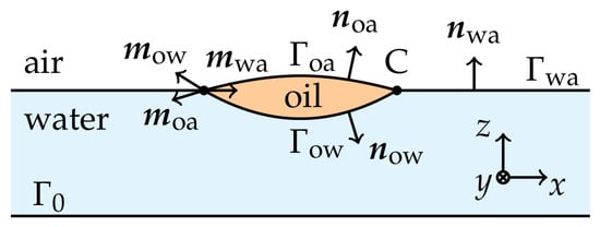
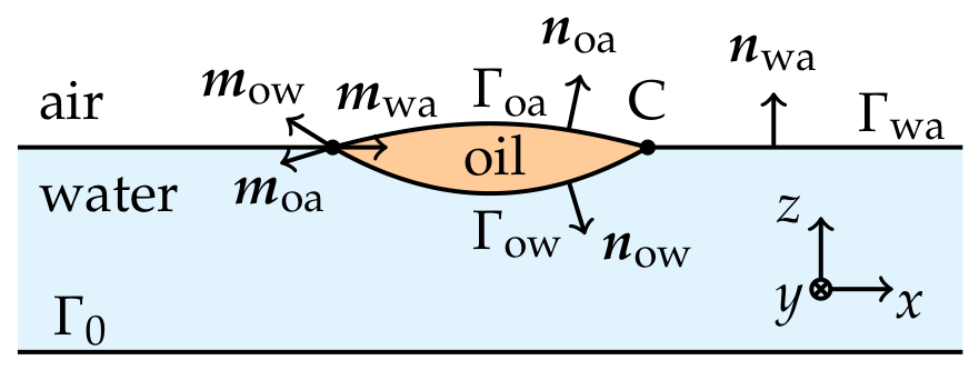
We consider a three-dimensional problem of an oil droplet (o) floating on the interface between water (w) and air (a) phases, as schematically shown in Figure 1. Let ${\mathrm{\Gamma }}_{\mathrm{wa}}$, ${\mathrm{\Gamma }}_{\mathrm{ow}}$, and ${\mathrm{\Gamma }}_{\mathrm{oa}}$ be the water–air interface, the oil–water interface, and the oil–air interface. The entire system is enclosed by a solid wall (${\mathrm{\Gamma }}_0$), including the bottom surface of the water phase, where we assume a no-slip boundary condition. The unit normal vectors (${\mathit{n}}_{\mathrm{wa}}$, ${\mathit{n}}_{\mathrm{ow}}$, and ${\mathit{n}}_{\mathrm{oa}}$) and unit conormal vectors (${\mathit{m}}_{\mathrm{wa}}$, ${\mathit{m}}_{\mathrm{ow}}$, and ${\mathit{m}}_{\mathrm{oa}}$) for the respective interfaces are defined as shown in Figure 1. The three-phase contact line is denoted by C.

Figure 1. Cross-sectional schematic of a droplet floating at the water–air interface. In Section 2.2, the droplet is treated as a general three-dimensional lens-shaped body. In Section 2.3, it is modeled as an infinitely long body with a uniform cross-section so that the problem becomes effectively one-dimensional. The water–air, oil–water, and oil–air interfaces are denoted by ${\mathrm{\Gamma }}_{\mathrm{wa}}$, ${\mathrm{\Gamma }}_{\mathrm{ow}}$, and ${\mathrm{\Gamma }}_{\mathrm{oa}}$, respectively. Their unit normal vectors (${\mathit{n}}_{\mathrm{wa}}$, ${\mathit{n}}_{\mathrm{ow}}$, and ${\mathit{n}}_{\mathrm{oa}}$) and their unit conormal vectors (${\mathit{m}}_{\mathrm{wa}}$, ${\mathit{m}}_{\mathrm{ow}}$, and ${\mathit{m}}_{\mathrm{oa}}$) are defined as in the figure. The entire system is enclosed by solid walls denoted by ${\mathrm{\Gamma }}_0$, where a no-slip boundary condition applies. C denotes the three-phase contact line.

2.2. Steady Propulsion of a Droplet

We now consider the steady propulsion of a three-dimensional droplet with a lens-like shape at the water–air interface, driven by a gradient in the interfacial tension (${\gamma }_{\mathrm{wa}}$) on ${\mathrm{\Gamma }}_{\mathrm{wa}}$, where the droplet moves at a constant velocity (v). Our goal in this section is to express v in terms of the ${\gamma }_{\mathrm{wa}}$ profile by using the Lorentz reciprocal theorem [25,26]. This framework has been widely used to analyze Marangoni-driven propulsion at fluid interfaces [27,28,29].

It should be noted that, as shown later, the Reynolds number under typical experimental conditions is of order unity, i.e., $\mathrm{Re}$∼1. However, Kang et al. reported that the flow field at $\mathrm{Re}$∼1 is only weakly modified relative to its low-Re counterpart, while the characteristic Marangoni-driven flow topology is preserved [29]. This suggests that our reciprocal-theorem-based model may still serve as a useful qualitative framework for relating the propulsion velocity to the interfacial-tension distribution, even when $\mathrm{Re}$∼1.

Provided that the two Stokes-flow problems are defined in the same domains with identical interfacial shapes, the Lorentz reciprocal theorem for the three phases ($p=\mathrm{w},\mathrm{o},\mathrm{a}$) can be written as

$$\begin{array}{cc}\hfill \sum _{p=\mathrm{w},\mathrm{o},\mathrm{a}}{\int }_{\partial {\mathrm{\Omega }}_p}[{\mathit{u}}_p^{\ast }·\left({\mathit{\sigma }}_p{\mathit{n}}_p\right)-{\mathit{u}}_p·\left({\mathit{\sigma }}_p^{\ast }{\mathit{n}}_p\right)]\mathrm{d}S& =\sum _{p=\mathrm{w},\mathrm{o},\mathrm{a}}{\int }_{{\mathrm{\Omega }}_p}({\mathit{f}}_p^{\ast }·{\mathit{u}}_p-{\mathit{f}}_p·{\mathit{u}}_p^{\ast })\mathrm{d}V,\hfill \end{array}$$

(1)

where ${\mathrm{\Omega }}_p$ denotes the domain occupied by phase p, $\partial {\mathrm{\Omega }}_p$ is its boundary, and ${\mathit{n}}_p$ is the outward unit normal on $\partial {\mathrm{\Omega }}_p$. The $({\mathit{u}}_p,{\mathit{\sigma }}_p,{\mathit{f}}_p)$ and $({\mathit{u}}_p^{\ast },{\mathit{\sigma }}_p^{\ast },{\mathit{f}}_p^{\ast })$ fields denote the velocity field, stress field, and prescribed body-force density appearing in the two Stokes problems defined in the ${\mathrm{\Omega }}_p$ domain. The ${\kappa }_{\mathrm{wa}}$, ${\kappa }_{\mathrm{ow}}$, and ${\kappa }_{\mathrm{oa}}$ curvatures for the ${\mathrm{\Gamma }}_{\mathrm{wa}}$, ${\mathrm{\Gamma }}_{\mathrm{ow}}$, and ${\mathrm{\Gamma }}_{\mathrm{oa}}$ interfaces, respectively, are common between the two problems. We assume that ${\mathrm{\Gamma }}_{\mathrm{wa}}$ is flat, that is, ${\kappa }_{\mathrm{wa}}=0$. We also assume that all interfaces are hydrodynamically impermeable and that the velocity fields are continuous on the interfaces.

In the primary problem $({\mathit{u}}_p,{\mathit{\sigma }}_p,{\mathit{f}}_p)$, we define the interfacial tensions, (${\gamma }_{\mathrm{wa}}$, ${\gamma }_{\mathrm{ow}}$, and ${\gamma }_{\mathrm{oa}}$) and the interfacial flow fields (${\mathit{u}}_{\mathrm{wa}}$, ${\mathit{u}}_{\mathrm{ow}}$, and ${\mathit{u}}_{\mathrm{oa}}$) for the interfaces (${\mathrm{\Gamma }}_{\mathrm{wa}}$, ${\mathrm{\Gamma }}_{\mathrm{ow}}$, and ${\mathrm{\Gamma }}_{\mathrm{oa}}$, respectively). We assume that the oil is mildly surface-active and dissolves into the aqueous phase, thereby reducing ${\gamma }_{\mathrm{wa}}$. The reduction in ${\gamma }_{\mathrm{wa}}$ may be spatially asymmetric along ${\mathrm{\Gamma }}_{\mathrm{wa}}$. On the other hand, we assume that ${\mathrm{\Gamma }}_{\mathrm{ow}}$ and ${\mathrm{\Gamma }}_{\mathrm{oa}}$ are homogeneous, that is, their interfacial tensions are constants. Therefore, we have

$$\begin{array}{ccc}\hfill {\nabla }_s{\gamma }_{\mathrm{wa}}& \ne 0,\hfill & \hfill {\nabla }_s{\gamma }_{\mathrm{ow}}={\nabla }_s{\gamma }_{\mathrm{oa}}=0,\end{array}$$

(2)

where ${\nabla }_s$ denotes the surface gradient on the interface. The inhomogeneous ${\gamma }_{\mathrm{wa}}$ induces the Marangoni stress acting along ${\mathrm{\Gamma }}_{\mathrm{wa}}$, breaks the symmetry, and drives the droplet in the direction of ${\mathit{e}}_x$ (${\mathit{e}}_x·{\mathit{n}}_{\mathrm{wa}}=0$) with constant velocity ($v{\mathit{e}}_x$), with no external body force applied (${\mathit{f}}_p=0$). Since the interfaces do not change their shapes, we have the following conditions:

$$\begin{array}{cccc}\hfill {\mathit{u}}_{\mathrm{ow}}·{\mathit{n}}_{\mathrm{ow}}& =v{\mathit{e}}_x·{\mathit{n}}_{\mathrm{ow}},\hfill & \hfill {\mathit{u}}_{\mathrm{oa}}·{\mathit{n}}_{\mathrm{oa}}& =v{\mathit{e}}_x·{\mathit{n}}_{\mathrm{oa}}.\hfill \end{array}$$

(3)

We also assume local mechanical equilibrium at the three-phase contact line, even when the droplet is moving, so that the Neumann condition on C holds:

$$\begin{array}{cc}\hfill {\gamma }_{\mathrm{wa}}{\mathit{m}}_{\mathrm{wa}}+{\gamma }_{\mathrm{ow}}{\mathit{m}}_{\mathrm{ow}}+{\gamma }_{\mathrm{oa}}{\mathit{m}}_{\mathrm{oa}}& =0.\hfill \end{array}$$

(4)

The droplet remains force-free at every instant in the Stokes limit, i.e., the net hydrodynamic force on the droplet vanishes. Here, “force-free” does not imply that the droplet–fluid subsystem is isolated: in the present finite-depth geometry, the no-slip bottom boundary sustains the stresses transmitted through the Marangoni-driven flow. In steady propulsion, a gradient of ${\gamma }_{\mathrm{wa}}$ produces a Marangoni stress that drives an interfacial flow, with this stress balanced by viscous stresses in the water phase. The droplet is carried by the resulting flow, like a surfer, while remaining free of a net horizontal capillary force.

In the auxiliary problem $({\mathit{u}}_p^{\ast },{\mathit{\sigma }}_p^{\ast },{\mathit{f}}_p^{\ast })$, on the other hand, the droplet does not dissolve, but it translates with a velocity of $v_0{\mathit{e}}_x$ under an external body-force density (${\mathit{f}}_{\mathrm{o}}^{\ast }$) acting on ${\mathrm{\Omega }}_{\mathrm{o}}$, while the shapes of the interfaces are kept identical to those in the primary problem. All the interfacial tensions (${\gamma }_{\mathrm{wa}}^{\ast }$, ${\gamma }_{\mathrm{ow}}^{\ast }$, and ${\gamma }_{\mathrm{oa}}^{\ast }$) are spatially uniform, i.e.,

$$\begin{array}{cc}\hfill {\nabla }_s{\gamma }_{\mathrm{wa}}^{\ast }& ={\nabla }_s{\gamma }_{\mathrm{ow}}^{\ast }={\nabla }_s{\gamma }_{\mathrm{oa}}^{\ast }=0.\hfill \end{array}$$

(5)

Let ${\mathit{u}}_{\mathrm{wa}}^{\ast }$, ${\mathit{u}}_{\mathrm{ow}}^{\ast }$, and ${\mathit{u}}_{\mathrm{oa}}^{\ast }$ be the interfacial flow fields for the respective interfaces; then, we have

$$\begin{array}{cccc}\hfill {\mathit{u}}_{\mathrm{ow}}^{\ast }·{\mathit{n}}_{\mathrm{ow}}& =v_0{\mathit{e}}_x·{\mathit{n}}_{\mathrm{ow}},\hfill & \hfill {\mathit{u}}_{\mathrm{oa}}^{\ast }·{\mathit{n}}_{\mathrm{oa}}& =v_0{\mathit{e}}_x·{\mathit{n}}_{\mathrm{oa}},\hfill \end{array}$$

(6)

and the Neumann condition on C is

$$\begin{array}{cc}\hfill {\gamma }_{\mathrm{wa}}^{\ast }{\mathit{m}}_{\mathrm{wa}}+{\gamma }_{\mathrm{ow}}^{\ast }{\mathit{m}}_{\mathrm{ow}}+{\gamma }_{\mathrm{oa}}^{\ast }{\mathit{m}}_{\mathrm{oa}}& =0.\hfill \end{array}$$

(7)

Since the interfacial unit normal vectors defined in Figure 1 do not, in general, coincide with the outward unit normal vectors of the ${\mathrm{\Omega }}_p$ domains, stress-jump terms arise on each interface. The stress-jump condition at the interface (${\mathrm{\Gamma }}_{pq}$) between phases p and q is

$$\begin{array}{cc}\hfill ({\mathit{\sigma }}_p-{\mathit{\sigma }}_q)·{\mathit{n}}_{pq}& =-{\gamma }_{pq}{\kappa }_{pq}{\mathit{n}}_{pq}+{\nabla }_s{\gamma }_{pq}\hfill \end{array}$$

(8)

where ${\mathit{n}}_{pq}$ is the unit normal vector pointing from phase p to phase q and ${\gamma }_{pq}$ and ${\kappa }_{pq}={\nabla }_s·{\mathit{n}}_{pq}$ denote the interfacial tension and curvature of ${\mathrm{\Gamma }}_{pq}$, respectively.

Using the definitions of the unit normal vectors shown in Figure 1, together with Equations (2), (5) and (8), the reciprocal relation (1) can be rewritten as

$$\begin{array}{cc}\hfill & {\int }_{{\mathrm{\Gamma }}_{\mathrm{ow}}}[-{\mathit{u}}_{\mathrm{ow}}^{\ast }·\left({\gamma }_{\mathrm{ow}}{\kappa }_{\mathrm{ow}}{\mathit{n}}_{\mathrm{ow}}\right)+{\mathit{u}}_{\mathrm{ow}}·\left({\gamma }_{\mathrm{ow}}^{\ast }{\kappa }_{\mathrm{ow}}{\mathit{n}}_{\mathrm{ow}}\right)]\mathrm{d}S\hfill \\ \hfill & +{\int }_{{\mathrm{\Gamma }}_{\mathrm{oa}}}[-{\mathit{u}}_{\mathrm{oa}}^{\ast }·\left({\gamma }_{\mathrm{oa}}{\kappa }_{\mathrm{oa}}{\mathit{n}}_{\mathrm{oa}}\right)+{\mathit{u}}_{\mathrm{oa}}·\left({\gamma }_{\mathrm{oa}}^{\ast }{\kappa }_{\mathrm{oa}}{\mathit{n}}_{\mathrm{oa}}\right)]\mathrm{d}S\hfill \\ \hfill & +{\int }_{{\mathrm{\Gamma }}_{\mathrm{wa}}}{\mathit{u}}_{\mathrm{wa}}^{\ast }·{\nabla }_s{\gamma }_{\mathrm{wa}}\mathrm{d}S={\int }_{{\mathrm{\Omega }}_{\mathrm{o}}}{\mathit{f}}_{\mathrm{o}}^{\ast }·{\mathit{u}}_{\mathrm{o}}\mathrm{d}V.\hfill \end{array}$$

(9)

Using the identity for an interfacial patch ($\mathrm{\Gamma }$) with a boundary of $\partial \mathrm{\Gamma }$,

$$\begin{array}{cc}\hfill {\int }_{\mathrm{\Gamma }}\kappa \mathit{n}\mathrm{d}S& =-{\oint }_{\partial \mathrm{\Gamma }}\mathit{m}\mathrm{d}l,\hfill \end{array}$$

(10)

and the conditions of (3), (4), (6), and (7), Equation (9) is further simplified as

$$\begin{array}{cc}\hfill -v_0{\mathit{e}}_x·{\oint }_C{\gamma }_{\mathrm{wa}}{\mathit{m}}_{\mathrm{wa}}\mathrm{d}l+v{\mathit{e}}_x·{\oint }_C{\gamma }_{\mathrm{wa}}^{\ast }{\mathit{m}}_{\mathrm{wa}}\mathrm{d}l+{\int }_{{\mathrm{\Gamma }}_{\mathrm{wa}}}{\mathit{u}}_{\mathrm{wa}}^{\ast }·{\nabla }_s{\gamma }_{\mathrm{wa}}\mathrm{d}S& ={\int }_{{\mathrm{\Omega }}_{\mathrm{o}}}{\mathit{f}}_{\mathrm{o}}^{\ast }·{\mathit{u}}_{\mathrm{o}}\mathrm{d}V.\hfill \end{array}$$

(11)

Now, because of (10) and ${\kappa }_{\mathrm{wa}}=0$, the second term in Equation (11) disappears:

$$\begin{array}{cc}\hfill {\oint }_C{\gamma }_{\mathrm{wa}}^{\ast }{\mathit{m}}_{\mathrm{wa}}\mathrm{d}l& ={\gamma }_{\mathrm{wa}}^{\ast }{\oint }_C{\mathit{m}}_{\mathrm{wa}}\mathrm{d}l=-{\gamma }_{\mathrm{wa}}^{\ast }{\int }_{{\mathrm{\Gamma }}_{\mathrm{wa}}}{\kappa }_{\mathrm{wa}}{\mathit{n}}_{\mathrm{wa}}\mathrm{d}S=0.\hfill \end{array}$$

(12)

Also, assuming that ${\mathit{f}}_{\mathrm{o}}^{\ast }$ is homogeneous in ${\mathrm{\Omega }}_{\mathrm{o}}$, we define ${\mathit{F}}_{\mathrm{o}}^{\ast }=\zeta v_0{\mathit{e}}_x$, with $\zeta$ being the drag coefficient, i.e.,

$$\begin{array}{cc}\hfill {\int }_{{\mathrm{\Omega }}_{\mathrm{o}}}{\mathit{f}}_{\mathrm{o}}^{\ast }·{\mathit{u}}_{\mathrm{o}}\mathrm{d}V& ={\mathit{F}}_{\mathrm{o}}^{\ast }·v{\mathit{e}}_x=\zeta v_{0}v,\hfill \end{array}$$

(13)

where

$$\begin{array}{cc}\hfill {\mathit{F}}_{\mathrm{o}}^{\ast }& =\zeta v_0{\mathit{e}}_x={\mathit{f}}_{\mathrm{o}}^{\ast }{\int }_{{\mathrm{\Omega }}_{\mathrm{o}}}\mathrm{d}V,v{\mathit{e}}_x={\displaystyle \frac{{\int }_{{\mathrm{\Omega }}_{\mathrm{o}}}{\mathit{u}}_{\mathrm{o}}\mathrm{d}V}{{\int }_{{\mathrm{\Omega }}_{\mathrm{o}}}\mathrm{d}V}}.\hfill \end{array}$$

(14)

Finally, substituting (12) and (14) into (11), we have

$$\begin{array}{cc}\hfill \zeta v& =-{\mathit{e}}_x·{\oint }_C{\gamma }_{\mathrm{wa}}{\mathit{m}}_{\mathrm{wa}}\mathrm{d}l+{\displaystyle \frac{1}{v_0}}{\int }_{{\mathrm{\Gamma }}_{\mathrm{wa}}}{\mathit{u}}_{\mathrm{wa}}^{\ast }·{\nabla }_s{\gamma }_{\mathrm{wa}}\mathrm{d}S\hfill \end{array}$$

(15)

as the velocity equation for the self-propulsion of the droplet. The first term of the right-hand side represents the drag of ${\gamma }_{\mathrm{wa}}$ acting along C, whereas the second term represents the drive of the Marangoni stress on ${\mathrm{\Gamma }}_{\mathrm{wa}}$, weighted by ${\mathit{u}}_{\mathrm{wa}}^{\ast }$.

2.3. Long Cylindrical Droplet with a Lens-Shaped Cross-Section

In this section, we examine (15) more closely by modeling the droplet as an infinitely long cylinder with a lens-shaped cross-section (Figure 1). The droplet is centered at the origin, and its long axis is aligned with the y-axis. In cross-section, it occupies the interval of $-a\le x\le a$ along the x-axis. Therefore, the problem is reduced to an effectively one-dimensional description along the x-axis, and the force acting on the droplet should be interpreted as the force per unit length. Then, Equation (15) is simplified as

$$\begin{array}{cc}\hfill \zeta v& =\gamma \left(a\right)-\gamma (-a)+{\displaystyle \frac{1}{v_0}}{\int }_{-\infty }^{-a}{u}^{\ast }\left(x\right){\displaystyle \frac{\mathrm{d}\gamma }{\mathrm{d}x}}\mathrm{d}x+{\displaystyle \frac{1}{v_0}}{\int }_a^{\infty }{u}^{\ast }\left(x\right){\displaystyle \frac{\mathrm{d}\gamma }{\mathrm{d}x}}\mathrm{d}x\hfill \end{array}$$

(16)

where $\gamma \left(x\right)$ and $u^{\ast }\left(x\right)$ are used for ${\gamma }_{\mathrm{wa}}$ and ${\mathit{u}}_{\mathrm{wa}}^{\ast }$, respectively.

To further simplify (16), we assume exponential decays for both $\gamma \left(x\right)$ and $u^{\ast }\left(x\right)$ as

$$\begin{array}{cc}\hfill \gamma \left(x\right)& =\left\{\begin{array}{cc}{\gamma }_0-\Delta {\gamma }_L\exp [(x+a)/{\lambda }_L]\hfill & (x<-a)\hfill \\ {\gamma }_0-\Delta {\gamma }_R\exp [-(x-a)/{\lambda }_R]\hfill & (x>a)\hfill \end{array}\right.\hfill \end{array}$$

(17)

$$\begin{array}{cc}\hfill u^{\ast }\left(x\right)& =\left\{\begin{array}{cc}{v}_0\exp [(x+a)/{\lambda }^{\ast }]\hfill & (x<-a)\hfill \\ v_0\exp [-(x-a)/{\lambda }^{\ast }]\hfill & (x>a),\hfill \end{array}\right.\hfill \end{array}$$

(18)

where ${\gamma }_0=\gamma (\pm \infty )$, $\Delta {\gamma }_L={\gamma }_0-\gamma (-a)$, and $\Delta {\gamma }_R={\gamma }_0-\gamma \left(a\right)$. ${\lambda }_L$ and ${\lambda }_R$ denote the relaxation lengths of the interfacial-tension profile on the left and right sides, respectively, whereas ${\lambda }^{\ast }$ denotes the characteristic decay length of the auxiliary velocity profile, which is symmetric about the droplet center, along the water–air interface. In a shallow water layer, ${\lambda }^{\ast }$ is expected to be controlled by the hydrodynamic screening due to the bottom wall and is therefore of the order of the water depth. The exponential forms in Equations (17) and (18) should be regarded as minimal phenomenological profiles that satisfy the boundary conditions with a finite relaxation length; these forms are motivated by the steady reaction–diffusion solution discussed below in Section 3.

Substituting (17) and (18) into (16) yields

$$\begin{array}{cc}\hfill \zeta v& =\gamma \left(a\right)-\gamma (-a)+{\displaystyle \frac{\Delta {\gamma }_R}{1+{\xi }_R}}-{\displaystyle \frac{\Delta {\gamma }_L}{1+{\xi }_L}},\hfill \end{array}$$

(19)

where ${\xi }_R={\lambda }_R/{\lambda }^{\ast }$ and ${\xi }_L={\lambda }_L/{\lambda }^{\ast }$. When ${\xi }_R\gg 1$ and ${\xi }_L\gg 1$, Equation (19) becomes

$$\begin{array}{cc}\hfill v& \simeq {\displaystyle \frac{\gamma \left(a\right)-\gamma (-a)}{\zeta }}.\hfill \end{array}$$

(20)

Therefore, the droplet is propelled by the difference in $\gamma$ between its two edges. On the other hand, if ${\xi }_R\ll 1$ and ${\xi }_L\ll 1$, Equation (19) becomes

$$\begin{array}{cc}\hfill v& \simeq 0.\hfill \end{array}$$

(21)

When, for example, ${\xi }_R\simeq {\xi }_L\simeq 1$,

$$\begin{array}{cc}\hfill v& \simeq {\displaystyle \frac{\gamma \left(a\right)-\gamma (-a)}{2\zeta }}.\hfill \end{array}$$

(22)

These results suggest that the droplet is propelled primarily by the difference in $\gamma$ between its two edges, while the Marangoni stress acts as a brake on the propulsion.

3. Effective Equation of Motion

In Section 2, we derived hydrodynamic closure relations in the Stokes limit. Equation (15) applies to a three-dimensional droplet, whereas Equation (16) represents its effectively one-dimensional reduction along the direction of motion. In this section, we no longer attempt to derive the dynamics from the detailed geometry of the droplet and the surrounding interfaces. Instead, we construct a coarse-grained one-dimensional dynamical model in which $\zeta$ is treated as an effective drag coefficient of the droplet.

We combine the hydrodynamic closure obtained in Section 2 with a minimal model for the effective propulsive force ($\kappa \Delta \gamma$) by writing

$$\begin{array}{cc}\hfill m\dot{v}& =-\zeta v+\kappa \Delta \gamma ,\hfill \end{array}$$

(23)

where $\Delta \gamma =\gamma \left(a\right)-\gamma (-a)$ denotes the difference in $\gamma \left(x\right)$ between the two edges of the droplet and $\kappa$ accounts for both the geometrical effects of the droplet and the effects of relaxation lengths along the interfaces.

The two points ($x=\pm a$) used in Equations (16) and (19) should be regarded as a reduced representation of the front and rear portions of the contact line (C) of a three-dimensional droplet. In this sense, the scalar driving term ($\kappa \Delta \gamma$) introduced here is a one-dimensional projection of the vectorial capillary–Marangoni driving in Equation (15). As shown above, its leading contribution is expected to be governed by the front–rear or first polar asymmetry of the interfacial-tension field around the contact line. The quantity ($\Delta \gamma$) used below should therefore be interpreted as a one-dimensional proxy for this leading asymmetric mode.

Similarly, $m\dot{v}$ in Equation (23) should not be interpreted as literal inertia; rather, (23) is introduced as an effective evolution equation for v. In the overdamped limit ($m\to 0$), (23) recovers the instantaneous proportionality ($v\propto \Delta \gamma$), consistent with (19). Hereafter, we assume a linear relation between the concentration field ($c(x,t)$) of surface-active molecules and $\gamma (x,t)$ of the following form:

$$\begin{array}{cc}\hfill \gamma (x,t)& ={\gamma }_0-{\gamma }_1{\displaystyle \frac{c(x,t)}{c_0}},\hfill \end{array}$$

(24)

where ${\gamma }_0$, ${\gamma }_1$, and $c_0$ are constants.

3.1. Source of Air–Water Interfacial Tension Gradient

We consider a droplet translating along a one-dimensional coordinate (x) with a position of $X\left(t\right)$. The droplet releases surface-active molecules that modify the local surface tension according to Equation (24). As a minimal description, we model $c(x,t)$ using the reaction–diffusion equation [1,5,28,30,31,32], i.e.,

$$\begin{array}{cc}\hfill {\displaystyle \frac{\partial c}{\partial t}}& =D{\displaystyle \frac{{\partial }^{2}c}{\partial x^2}}-bc,\hfill \end{array}$$

(25)

where D is the diffusion coefficient and b is an effective first-order decay rate (e.g., dissolution into the bulk or evaporation).

The supply of the surfactant from the droplet is represented by the Dirichlet condition, i.e.,

$$\begin{array}{cc}\hfill c\left(X\right(t),t)& =c_0,\hfill \end{array}$$

(26)

with $c_0$ being a constant, that is, we prescribe the concentration at the droplet position of $x=X\left(t\right)$. Equation (26) represents an idealized reservoir condition at the droplet, i.e., rapid local equilibration that fixes the interfacial concentration.

This one-dimensional model should be regarded as a coarse-grained effective description that accounts for the edge-localized surface-tension gradient. Although the droplet is represented as a pointwise reservoir in the concentration field, the values of $c(\pm a)$ are interpreted as effective proxies for the concentration values near the front and rear edges of a finitely sized droplet. Therefore, the model does not resolve the contact-line scale structure explicitly, but it captures the resulting edge-to-edge difference in the surface-tension field that drives the droplet motion.

To analyze the concentration profile in the droplet frame, we introduce the comoving coordinate ($s=x-X\left(t\right)$) and define $\tilde{c}(s,t)=c(x,t)$. Using ${\partial }_{t}c={\partial }_t\tilde{c}-\dot{X}{\partial }_s\tilde{c}$, and ${\partial }_{x}c={\partial }_s\tilde{c}$, Equation (25) can be rewritten (dropping the tilde for simplicity) as

$$\begin{array}{cc}\hfill {\displaystyle \frac{\partial c}{\partial t}}-v{\displaystyle \frac{\partial c}{\partial s}}& =D{\displaystyle \frac{{\partial }^{2}c}{\partial s^2}}-bc,\hfill \end{array}$$

(27)

where $v=\dot{X}$.

3.2. Steady State

Following a previous study [13], we next consider the steady state in the comoving frame, i.e., ${\partial }_{t}c=0$. Then Equation (27) reduces to the following ordinary differential equation:

$$\begin{array}{cc}\hfill D{c}^{″}+v{c}^{\prime }-bc& =0.\hfill \end{array}$$

(28)

The general solution to (28) is

$$\begin{array}{cc}\hfill c\left(s\right)& ={\mathrm{e}}^{-k_{0}s}(C_1{\mathrm{e}}^{k_{1}s}+C_2{\mathrm{e}}^{-k_{1}s})\hfill \end{array}$$

(29)

where $C_1$ and $C_2$ are constants and $k_0$ and $k_1$ are given by

$$\begin{array}{cc}\hfill k_0& ={\displaystyle \frac{v}{2D}},\hfill \end{array}$$

(30)

$$\begin{array}{cc}\hfill k_1& ={\displaystyle \frac{\sqrt{v^2+4bD}}{2D}}.\hfill \end{array}$$

(31)

Imposing the boundary conditions of $c\left(0\right)=c_0$ and $c(\pm \infty )=0$ yields the piecewise exponential profile:

$$\begin{array}{c}\hfill c\left(s\right)=\left\{\begin{array}{c}{c}_0{\mathrm{e}}^{k_{L}s},s<0,\hfill \\ c_0{\mathrm{e}}^{-k_{R}s},s>0,\hfill \end{array}\right.\end{array}$$

(32)

where $k_L=k_1-k_0$ and $k_R=k_1+k_0$.

3.3. Effective Equation of Motion

Using Equation (24), the effective equation of motion (23) becomes

$$\begin{array}{cc}\hfill m\dot{v}& =-\zeta v+2\kappa {\gamma }_1{\mathrm{e}}^{-k_{1}a}\sinh \left(k_{0}a\right).\hfill \end{array}$$

(33)

In the overdamped limit, (33) reduces to the instantaneous closure ($v\propto \Delta \gamma$). We non-dimensionalize (33) using $l_0=2a$ as the unit of length, $t_0=a^2/D$ as the unit of time, and m as the unit of mass. This yields

$$\begin{array}{cc}\hfill {\displaystyle \frac{\mathrm{d}\tilde{v}}{\mathrm{d}\tilde{t}}}& =-\tilde{\zeta }\tilde{v}+\tilde{\phi }{\mathrm{e}}^{-\sqrt{{\tilde{v}}^2+\tilde{b}}}\sinh \tilde{v}.\hfill \end{array}$$

(34)

The dimensionless parameters are defined as

$$\begin{array}{cc}\hfill \tilde{v}& ={\displaystyle \frac{a}{2D}}v,\hfill \end{array}$$

(35)

$$\begin{array}{cc}\hfill \tilde{\zeta }& ={\displaystyle \frac{a^2}{mD}}\zeta ,\hfill \end{array}$$

(36)

$$\begin{array}{cc}\hfill \tilde{b}& ={\displaystyle \frac{a^2}{D}}b,\hfill \end{array}$$

(37)

$$\begin{array}{cc}\hfill \tilde{\phi }& ={\displaystyle \frac{\kappa a^3{\gamma }_1}{m{D}^2}}.\hfill \end{array}$$

(38)

Here, $\tilde{v}$ is proportional to the Péclet number, whereas $\tilde{\phi }$ plays a role analogous to the Marangoni number. $\tilde{b}$ is the Damköhler number [33], and $\tilde{\zeta }$ is the ratio of the diffusion time (${\tau }_c=a^2/D$) to the Stokes time (${\tau }_v=m/\zeta$).

Let us give a rough estimate of the dimensionless values (see Supplementary Materials, Section SI). Assuming $\kappa$∼a and using v∼${10}^{-3}$ m/s, a∼${10}^{-3}$ m, D∼${10}^{-5}$ m²/s (as an effective diffusion coefficient [34]), m∼${10}^{-5}$ kg, $\zeta$∼${10}^{-5}$ Ns/m, ${\gamma }_1$∼${10}^{-3}$ N/m, and b∼${10}^{-2}$ s⁻¹ [35], we have $\tilde{v}$∼${10}^{-1}$, $\tilde{\zeta }$∼${10}^{-1}$, $\tilde{\phi }$∼1, and $\tilde{b}$∼${10}^{-3}$.

Strictly speaking, the driving $\kappa \Delta \gamma$ is derived from a steady advection–diffusion problem. Moreover, the typical Reynolds number, estimated as $\mathrm{Re}=va/\nu$ with a kinematic viscosity of $\nu$∼${10}^{-6}{\mathrm{m}}^2/\mathrm{s}$, is of order unity. Therefore, the Stokes-based derivation is not expected to be quantitatively accurate in detail, but it should still provide a useful qualitative constitutive relation between the propulsion velocity and the interfacial-tension difference [29]. Here, we extend it to time-dependent dynamics by assuming that the concentration field relaxes faster than the droplet velocity and can be treated as a function of the instantaneous droplet velocity. We therefore use the steady expression for $\Delta \gamma$ as a leading-order approximation. Since $\tilde{\zeta }={\tau }_c/{\tau }_v$∼$0.1$, non-quasi-steady effects on how the concentration field tracks the droplet velocity are expected to remain modest and to enter mainly through $O\left(\tilde{\zeta }\right)$ renormalizations of the coefficients rather than through qualitative changes in the dynamics.

The Schmidt number, i.e.,

$$\begin{array}{cc}\hfill \mathrm{Sc}& =\nu /D\sim 10,\hfill \end{array}$$

(39)

provides an estimate of the separation between ${\lambda }_R$, ${\lambda }_L$, and ${\lambda }^{\ast }$, as $\mathrm{Sc}$∼${\lambda }_R/{\lambda }^{\ast }$∼${\lambda }_L/{\lambda }^{\ast }$. $\mathrm{Sc}$∼10 suggests that ${\xi }_R$∼${\xi }_L$∼10 so that Equation (20) is practically valid under typical experimental settings.

We also estimate the capillary number ($\mathrm{Ca}$). Taking the viscosity, $\mu \simeq {10}^{-3}$ Pa·s, and ${\gamma }_0\simeq 30\times {10}^{-3}$ N/m, we obtain

$$\begin{array}{cc}\hfill \mathrm{Ca}& ={\displaystyle \frac{\mu v}{{\gamma }_0}}\sim {10}^{-5}.\hfill \end{array}$$

(40)

This suggests that the interfaces remain nearly flat under our conditions, although interfacial deformation near a self-propelled droplet has been observed experimentally [36].

Hereafter, we omit tildes and use the following dimensionless equation of motion:

$$\begin{array}{cc}\hfill \dot{v}& =-\zeta v+\phi {\mathrm{e}}^{-\sqrt{v^2+b}}\sinh v.\hfill \end{array}$$

(41)

Since (41) is symmetric under the transformation of $v\to -v$, it is expected to exhibit a pitchfork bifurcation.

3.4. Pitchfork Bifurcation

We examine the bifurcation around $v=0$ by expanding the right-hand side of (41) in a power series, retaining terms up to $O\left(v^3\right)$, i.e.,

$$\begin{array}{cc}\hfill \dot{v}& =(-\zeta +\alpha )v+\beta v^3,\hfill \end{array}$$

(42)

where

$$\begin{array}{cc}\hfill \alpha & =\phi {\mathrm{e}}^{-\sqrt{b}},\hfill \end{array}$$

(43)

$$\begin{array}{cc}\hfill \beta & ={\displaystyle \frac{\phi {\mathrm{e}}^{-\sqrt{b}}}{6}}(1-{\displaystyle \frac{3}{\sqrt{b}}}).\hfill \end{array}$$

(44)

Equation (42) is a normal form of the pitchfork bifurcation where the stationary fixed point ($v^{\ast }=0$) always exists and the two propulsive fixed points ($v^{\ast }=\pm v_p$) exist when $\zeta <{\zeta }_c=\alpha$ and $\beta <0$ or $\zeta >{\zeta }_c$ and $\beta >0$. The stationary fixed point is stable when $\zeta >{\zeta }_c$ and unstable when $\zeta <{\zeta }_c$. The bifurcation is supercritical when $\beta <0$ ($b<9$), that is, $\pm v_p$ are stable. When $\beta >0$ ($b>9$), the bifurcation is subcritical, that is, $\pm v_p$ exist, but they are unstable. For typical values, b∼${10}^{-3}$, so $\beta$∼$-15$; hence, the pitchfork bifurcation is expected to be supercritical.

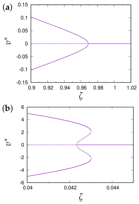
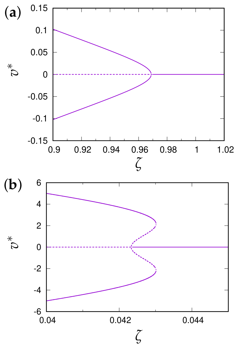
Returning to Equation (41), we first consider the supercritical bifurcation when $b<9$. It is possible to show that this supercritical pitchfork bifurcation is the only bifurcation under this condition. Figure 2a shows a typical bifurcation diagram obtained numerically for $\phi =1$ and $b={10}^{-3}$. The bifurcation point is ${\zeta }_c\simeq 0.9689$. The stationary fixed point ($v^{\ast }=0$) is stable for $\zeta >{\zeta }_c$ and becomes unstable for $\zeta <{\zeta }_c$, where propulsive fixed points ($v^{\ast }=\pm v_p$) emerge. This bifurcation indicates the onset of sustained self-propulsion once $\zeta$ falls below a threshold.

Figure 2. Bifurcation diagrams of Equation (41). $\phi =1$. (a) $b={10}^{-3}$ and (b) $b=10$. The solid lines represent stable fixed points, and the dashed lines represent unstable fixed points.

When $b>9$, Equation (42) has unstable branches that diverge to infinity. In the full system, (41), however, this divergence is avoided because stable branches generated by saddle-node bifurcations appear at finite values of v. Moreover, one finds that there are only two symmetric saddle-node bifurcations. Figure 2b shows a bifurcation diagram for $\phi =1$ and $b=10$. When $\zeta$ is decreased from $\zeta >{\zeta }_c={\mathrm{e}}^{-\sqrt{10}}\simeq 0.04233$, the stationary fixed point ($v^{\ast }=0$) remains stable until $\zeta ={\zeta }_c$. This bifurcation is a subcritical pitchfork bifurcation. Before this bifurcation, a pair of saddle-node bifurcations occurs at $\zeta \simeq 0.04301$, producing four nonzero fixed points—a stable $\pm v_1$ and an unstable $\pm v_2$ (with $|v_1|>|v_2|>0$)—in the interval between the saddle-node bifurcation and the subcritical pitchfork bifurcation.

This bifurcation structure implies that the droplet dynamics can become bistable (both $v^{\ast }=0$ and $v^{\ast }=\pm v_1$ are stable) over a finite range of $\zeta$ when b is large. Outside this range, only a single stable state remains, corresponding either to the stationary ($v^{\ast }=0$) or to sustained self-propulsion ($v^{\ast }=\pm v_1$), depending on the parameters.

4. A Dynamical Model of Droplet Self-Propulsion

4.1. Two-Variable Systems

Equation (42) is a one-variable reduced model that describes the onset of self-propulsion under the assumption that the effective driving adjusts quasi-steadily to the droplet velocity—namely, through the algebraic form of $\alpha v+\beta v^3$. To go beyond this quasi-steady description and allow for a finite response time of the driving, we now promote it to an internal dynamical variable ($f\left(t\right)$) and assume that it relaxes toward the quasi-steady value on a characteristic timescale ($\tau$):

$$\begin{array}{cc}\hfill \dot{v}& =-\zeta v+f,\hfill \end{array}$$

(45)

$$\begin{array}{cc}\hfill \dot{f}& ={\displaystyle \frac{1}{\tau }}(\alpha v+\beta v^3-f),\hfill \end{array}$$

(46)

where $\alpha$ and $\beta$ are given by (43) and (44). This provides the minimal dynamical extension of (42): it preserves the same symmetry and steady states, introduces only one additional variable and one additional timescale, and reduces to (42) in the fast-relaxation limit ($\tau \to 0$).

In previous studies, the force acting on the surfer was derived by expanding the concentration field in terms of the velocity and its higher-order time derivatives [37]. In that description, the force is given mainly by the velocity-dependent contribution, with additional corrections arising from these higher-order time derivatives. In contrast, in the present framework, such derivative-dependent corrections are not introduced explicitly. Instead, they are incorporated through relaxation dynamics in which the force evolves toward the steady-state value determined by the instantaneous velocity.

It is possible to show that there are no limit cycles in this system. Let

$$\begin{array}{cc}\hfill F_1(v,f)& =-\zeta v+f,\hfill \end{array}$$

(47)

$$\begin{array}{cc}\hfill F_2(v,f)& ={\displaystyle \frac{1}{\tau }}(\alpha v+\beta v^3-f).\hfill \end{array}$$

(48)

The divergence of the vector field ($\mathit{F}=(F_1,F_2)$) is

$$\begin{array}{cc}\hfill \nabla ·\mathit{F}& ={\displaystyle \frac{\partial F_1}{\partial v}}+{\displaystyle \frac{\partial F_2}{\partial f}}=-\zeta -{\displaystyle \frac{1}{\tau }}<0.\hfill \end{array}$$

(49)

Since the phase space is simply connected and $\nabla ·\mathit{F}<0$ holds everywhere, the Bendixson–Dulac criterion [38] excludes the existence of periodic orbits (limit cycles) in this two-variable system.

4.2. Three-Variable Systems

Since the two-variable system ((45) and (46)) admits no periodic orbits, it cannot produce sustained oscillatory dynamics such as back-and-forth motion. We therefore extend the model phenomenologically to the minimal symmetry-preserving three-variable form by introducing two distinct internal driving components: f and g.

$$\begin{array}{cc}\hfill \dot{v}& =-\zeta v+f+g,\hfill \end{array}$$

(50)

$$\begin{array}{cc}\hfill \dot{f}& ={\displaystyle \frac{1}{{\tau }_1}}({\alpha }_{1}v+{\beta }_1{v}^3-f),\hfill \end{array}$$

(51)

$$\begin{array}{cc}\hfill \dot{g}& ={\displaystyle \frac{1}{{\tau }_2}}({\alpha }_{2}v+{\beta }_2{v}^3-g),\hfill \end{array}$$

(52)

where ${\alpha }_1$, ${\alpha }_2$, ${\beta }_1$, and ${\beta }_2$ are constants and ${\tau }_1>0$ and ${\tau }_2>0$ are the relaxation times of the two force components. We also assume that ${\alpha }_1>0$ and ${\alpha }_2>0$.

The f and g variables are not meant to represent uniquely derived mechanical forces but effective Marangoni–hydrodynamic driving modes that coarse-grain the underlying interfacial dynamics. Physically, one may interpret them as two coarse-grained Marangoni driving modes with distinct response times. Experimentally, such a separation could arise from the coexistence of fast interfacial transport and slower bulk-mediated or adsorption–desorption dynamics. This should be understood as a minimal reduced description beyond the simplifying assumptions adopted in Section 2: the detailed interfacial hydrodynamics are not modeled explicitly but are incorporated effectively into the reduced f and g variables.

As before, there are two types of fixed points: stationary fixed points ($S=(0,0,0)$) and propulsive fixed points ($P=(v_p,f_p,g_p)$). The Jacobian is

$$\begin{array}{cc}\hfill J& =\left(\begin{array}{ccc}-\zeta & 1& 1\\ {\displaystyle \frac{{\alpha }_1+3{\beta }_1{v}^2}{{\tau }_1}}& -{\displaystyle \frac{1}{{\tau }_1}}& 0\\ {\displaystyle \frac{{\alpha }_2+3{\beta }_2{v}^2}{{\tau }_2}}& 0& -{\displaystyle \frac{1}{{\tau }_2}}\end{array}\right).\hfill \end{array}$$

(53)

The characteristic equation is

$$\begin{array}{cc}\hfill {\lambda }^3+c_2{\lambda }^2+c_1\lambda +c_0& =0,\hfill \end{array}$$

(54)

where

$$\begin{array}{cc}\hfill c_0& ={\displaystyle \frac{1}{{\tau }_1{\tau }_2}}(\zeta -A_1-A_2),\hfill \end{array}$$

(55)

$$\begin{array}{cc}\hfill c_1& =\zeta ({\displaystyle \frac{1}{{\tau }_1}}+{\displaystyle \frac{1}{{\tau }_2}})+{\displaystyle \frac{1}{{\tau }_1{\tau }_2}}-{\displaystyle \frac{A_1}{{\tau }_1}}-{\displaystyle \frac{A_2}{{\tau }_2}},\hfill \end{array}$$

(56)

$$\begin{array}{cc}\hfill c_2& =\zeta +{\displaystyle \frac{1}{{\tau }_1}}+{\displaystyle \frac{1}{{\tau }_2}},\hfill \end{array}$$

(57)

and

$$\begin{array}{cc}\hfill A_1& ={\alpha }_1+3{\beta }_1{v}^2,A_2={\alpha }_2+3{\beta }_2{v}^2.\hfill \end{array}$$

(58)

The conditions under which all roots of (54) have negative real parts are the following (given $c_2>0$) [39]:

$$\begin{array}{cc}\hfill c_0& >0,\hfill \end{array}$$

(59)

$$\begin{array}{cc}\hfill c_1& >0,\hfill \end{array}$$

(60)

$$\begin{array}{cc}\hfill c_1{c}_2& >c_0.\hfill \end{array}$$

(61)

The stationary fixed point (S) always exists. For S, (59) is satisfied if

$$\begin{array}{cc}\hfill \zeta & >{\alpha }_1+{\alpha }_2.\hfill \end{array}$$

(62)

Moreover, if $\zeta >{\alpha }_1+{\alpha }_2$, then (60) and (61) are also satisfied; hence, S is linearly stable when (62) holds.

On the other hand, the linear stability conditions for the propulsive fixed point (P), i.e.,

$$\begin{array}{cc}\hfill v_p& =\pm \sqrt{{\displaystyle \frac{\zeta -{\alpha }_1-{\alpha }_2}{{\beta }_1+{\beta }_2}}},\hfill \end{array}$$

(63)

$$\begin{array}{cc}\hfill f_p& ={\alpha }_1{v}_p+{\beta }_1{v}_p^3,\hfill \end{array}$$

(64)

$$\begin{array}{cc}\hfill g_p& ={\alpha }_2{v}_p+{\beta }_2{v}_p^3,\hfill \end{array}$$

(65)

are not simple. For P to exist and satisfy $c_0>0$, the necessary conditions are

$$\begin{array}{cc}\hfill {\alpha }_1+{\alpha }_2& >\zeta ,\hfill \end{array}$$

(66)

$$\begin{array}{cc}\hfill {\beta }_1+{\beta }_2& <0.\hfill \end{array}$$

(67)

We now choose a representative set of parameters to examine how the system behaves as these parameters are varied. For this purpose, we rewrite the system into a form that makes the physical meaning of the parameters more transparent:

$$\begin{array}{cc}\hfill \dot{v}& =-{\displaystyle \frac{v}{{\tau }_0}}+f+g,\hfill \end{array}$$

(68)

$$\begin{array}{cc}\hfill \dot{f}& =-{\displaystyle \frac{f}{{\tau }_1}}+{\mu }_1(v_1^2-v^2)v,\hfill \end{array}$$

(69)

$$\begin{array}{cc}\hfill \dot{g}& =-{\displaystyle \frac{g}{{\tau }_2}}+{\mu }_2(v_2^2-v^2)v,\hfill \end{array}$$

(70)

where ${\tau }_0=1/\zeta >0$, ${\mu }_1=-{\beta }_1/{\tau }_1$, ${\mu }_2=-{\beta }_2/{\tau }_2$, $v_1^2=-{\alpha }_1/{\beta }_1$, and $v_2^2=-{\alpha }_2/{\beta }_2$. We assume ${\beta }_1<0$ and ${\beta }_2<0$. Here, $v_1$ and $v_2$ represent the target speeds associated with the driving forces (f and g, respectively), while ${\mu }_1$ and ${\mu }_2$ quantify the strength of relaxation toward those target speeds.

It can be shown that, whenever it exists, P is stable in several simplified cases, including

• ${\tau }_1={\tau }_2$;
• $v_1=v_2$;
• ${\mu }_1={\mu }_2$, $v_1^2>v_2^2$ and ${\tau }_1>{\tau }_2$; or
• ${\mu }_1={\mu }_2$, $v_1^2>v_2^2$ and $3{\tau }_1>{\tau }_2>{\tau }_1$.

In addition, P is always stable when it is close enough to the bifurcation from S.

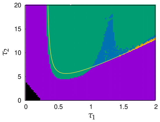
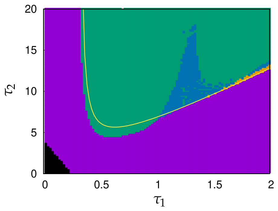
Interesting behavior is observed when P is destabilized. Therefore, we choose a parameter set (${\tau }_0=1$, ${\mu }_1={\mu }_2=1$, $v_1=2$, and $v_2=0.5$) and examine the effect of ${\tau }_1$ and ${\tau }_2$ on P. Figure 3 shows the results of numerical simulations. We started the simulations from the same initial condition, $v\left(0\right)={10}^{-3}$ and $f\left(0\right)=g\left(0\right)=0$.

Figure 3. Bifurcation diagrams obtained by numerically integrating (68)–(70) in the $({\tau }_1,{\tau }_2)$ plane for ${\tau }_0=1$, ${\mu }_1={\mu }_2=1$, $v_1=2$, and $v_2=0.5$. Black indicates the region where propulsive fixed points do not exist. Purple indicates stable fixed points (steady propulsion). Green indicates limit cycles that span both signs of v (back-and-forth motion). Blue indicates chaotic motion. Orange indicates limit cycles that remain on one side of $v=0$ (unidirectional motion with speed oscillations). The solid curve denotes the Hopf boundary (${\tau }_2^H\left({\tau }_1\right)$) defined by the condition of $c_1{c}_2=c_0$. Simulations were performed from the initial condition of $v={10}^{-3}$ with $f=g=0$.

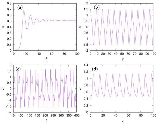
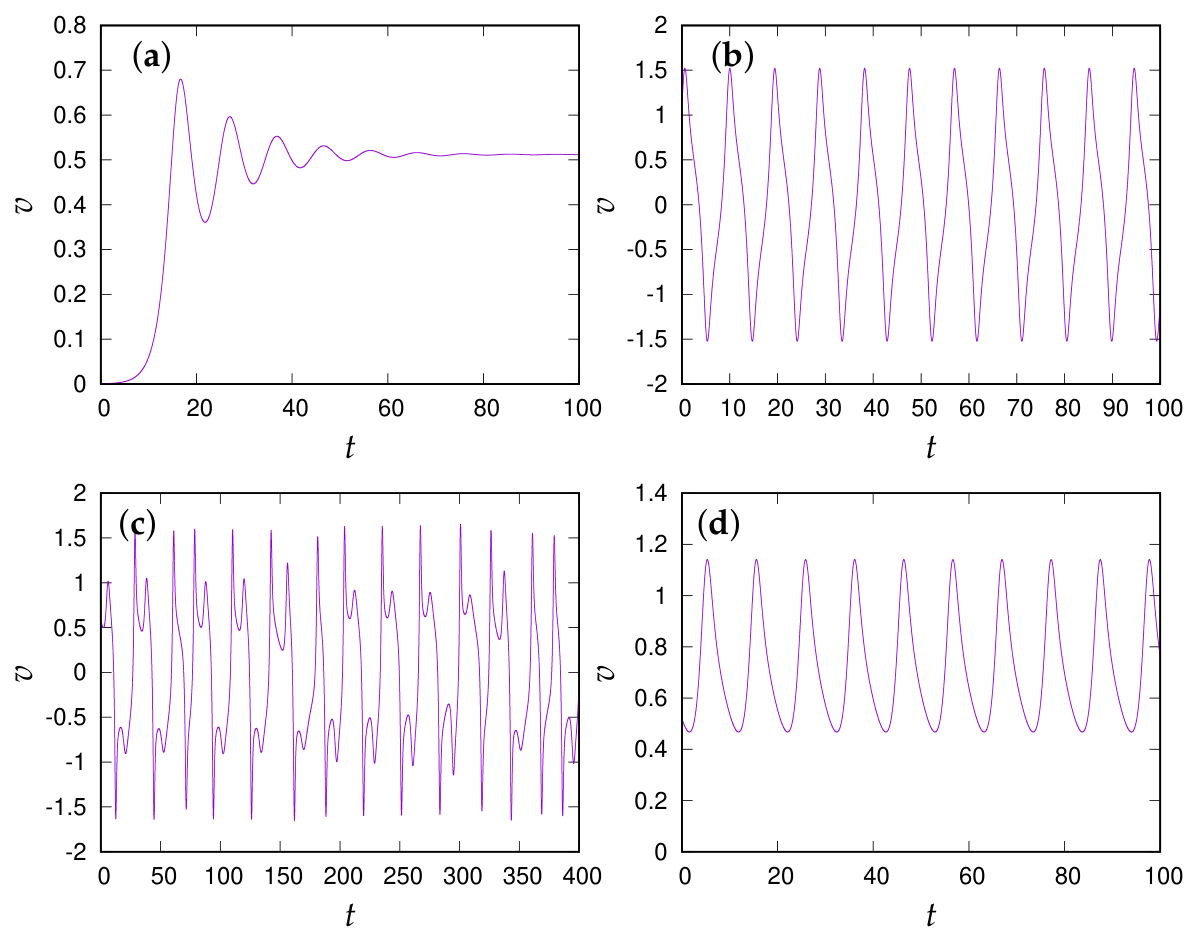
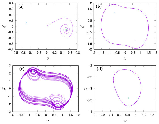
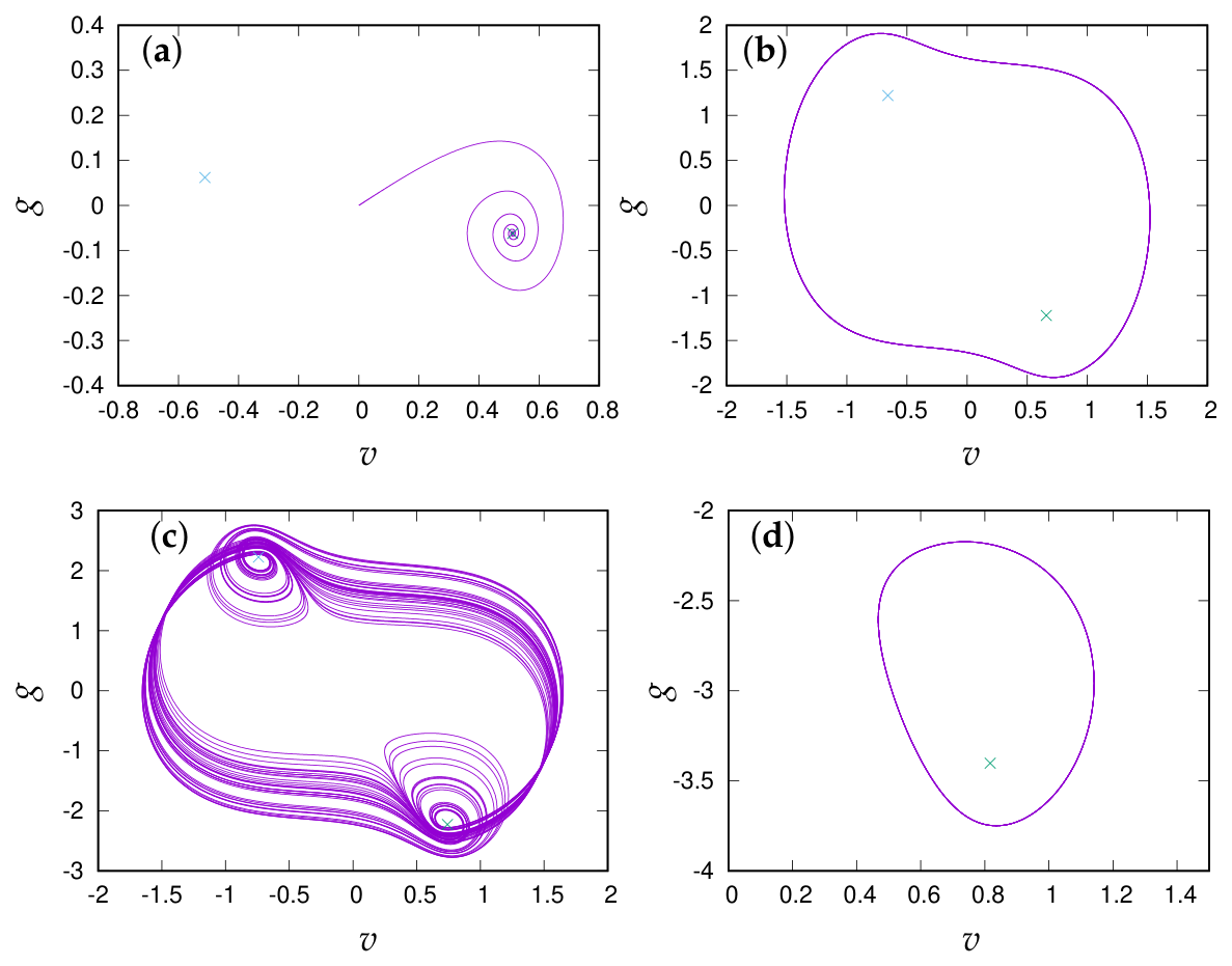
There are four types of dynamical behavior shown in Figure 3, along with their time series (Figure 4) and trajectories (Figure 5): stable fixed points (stable propulsion), limit cycles spanning both positive and negative velocities (back-and-forth motion), chaotic dynamics, and limit cycles confined to one side of $v=0$ (vibration in v). We classified the trajectory as a limit cycle when the amplitude of oscillation in v was larger than ${10}^{-3}$. The solid curve in Figure 3 indicates the Hopf boundary, i.e., ${\tau }_2^H\left({\tau }_1\right)$ (see Supplementary Materials, Section SIII).

Figure 4. Simulated time series of v for ${\tau }_0=1$, ${\tau }_2=10$, ${\mu }_1={\mu }_2=1$, $v_1=2$, and $v_2=0.5$. (a) ${\tau }_1=0.3$ (steady propulsion); (b) ${\tau }_1=0.8$ (back-and-forth motion); (c) ${\tau }_1=1.16$ (chaotic motion); (d) ${\tau }_1=1.55$ (unidirectional motion with speed oscillations). The initial state of the simulations was $v={10}^{-3}$ and $f=g=0$. The largest estimated Lyapunov exponents were $\lambda =-7.7\times {10}^{-2}$ for (a), $\lambda =6.5\times {10}^{-4}$ for (b), $\lambda =3.3\times {10}^{-2}$ for (c), and $\lambda =4.9\times {10}^{-4}$ for (d).

Figure 5. Phase trajectories in the v–g plane for ${\tau }_0=1$, ${\tau }_2=10$, ${\mu }_1={\mu }_2=1$, $v_1=2$, and $v_2=0.5$. (a) ${\tau }_1=0.3$ (steady propulsion); (b) ${\tau }_1=0.8$ (back-and-forth motion); (c) ${\tau }_1=1.16$ (chaotic motion); (d) ${\tau }_1=1.55$ (unidirectional motion with speed oscillations). Crosses indicate fixed points.

Chaotic trajectories can be viewed as irregular motion that does not converge to a closed orbit. The presence of chaos is supported by a positive finite-time Lyapunov exponent exceeding ${10}^{-3}$, computed using the standard QR method [40] (see Supplementary Materials, Section SV).

To further characterize these dynamics, we also calculated the power spectra of the velocity time series shown in Figure 4. The power spectra are shown in Supplementary Materials, Section SVI. The spectrum for Figure 4c contains multiple pronounced peaks, indicating several characteristic time scales rather than simple periodic motion. Since Fourier spectra alone cannot distinguish quasiperiodic and chaotic dynamics unambiguously, we used the maximal Lyapunov exponent as the main diagnostic. The maximal Lyapunov exponent for Figure 4c is positive and exceeds the prescribed threshold of ${10}^{-3}$; together with the irregular temporal fluctuations of the trajectory, this supports the classification of this state as chaotic.

Overall, stable propulsion occurs when ${\tau }_1$ and/or ${\tau }_2$ are small. In contrast, large-amplitude limit cycles (back-and-forth motion) typically arise when the weaker driving component (g, associated with $v_2$) has a much longer relaxation time (${\tau }_2$) than the relaxation time (${\tau }_1$) of the stronger component (f, associated with $v_1>v_2$). The relaxation time of v (${\tau }_0$) appears to need to be comparable to ${\tau }_1$. Small-amplitude limit cycles (vibration in v) are observed only within a limited parameter range near the Hopf boundary. Chaotic motion also appears primarily near the Hopf boundary, although it can sometimes occur deep within the region of large-amplitude limit cycles.

It should be noted that the parameters in Equations (68)–(70), which are used in Figure 3, Figure 4 and Figure 5, are effective parameters of the reduced model. Microscopic and geometrical details of the original droplet system, such as the hydrodynamic mobility, interfacial transport, wetting properties, and spatial structure of the surface-tension field, are coarse-grained into the coefficients (${\tau }_i$, ${\mu }_i$, and $v_i$). Therefore, the results shown in Figure 3, Figure 4 and Figure 5 should be interpreted as representative dynamical behaviors in the effective parameter space rather than as quantitative predictions for one specific microscopic realization. In limiting regimes where these microscopic or geometrical details change qualitatively, the present coarse-grained description would no longer be sufficient, and a more complete continuum description would be required.

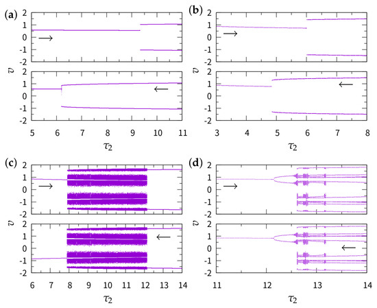
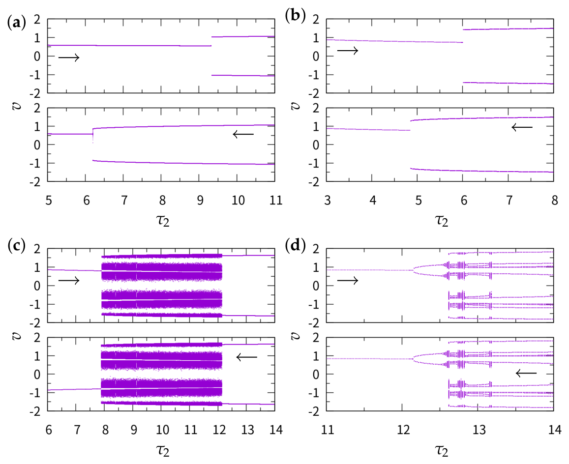
Figure 6 shows bifurcation diagrams in which the local extrema of v are plotted as a function of ${\tau }_2$ for several values of ${\tau }_1$. In the numerical simulations, the initial condition for each run is taken from the final state of the preceding run. In each panel, the upper branch corresponds to an increase in ${\tau }_2$ from its leftmost value, whereas the lower branch corresponds to a decrease in ${\tau }_2$ from its rightmost value.

Figure 6. Bifurcation diagrams: local extrema of v are plotted as a function of ${\tau }_2$. (a) ${\tau }_1=0.4$ (${\tau }_2^H\simeq 9.295$); (b) ${\tau }_1=0.8$ (${\tau }_2^H\simeq 6.007$); (c) ${\tau }_1=1.2$ (${\tau }_2^H\simeq 7.906$); (d) ${\tau }_1=1.9$ (${\tau }_2^H\simeq 12.141$). Other parameters are fixed as ${\tau }_0=1$, ${\mu }_1={\mu }_2=1$, $v_1=2.0$, and $v_2=0.5$. Arrows indicate the direction in which ${\tau }_2$ is varied. For each simulation, the initial condition is taken from the final state of the previous run.

For ${\tau }_1=0.4$ [Figure 6a] and ${\tau }_1=0.8$ [Figure 6b], a clear hysteresis is observed: stable limit cycles emerge at the Hopf bifurcation point (${\tau }_2^H$) when ${\tau }_2$ is increased, but they disappear at values significantly below ${\tau }_2^H$ when ${\tau }_2$ is decreased. This hysteresis indicates that the observed limit cycles are globally stable and persist even in a parameter regime where the fixed point (P) remains linearly stable.

The stability analysis of the Hopf bifurcation based on the Lyapunov coefficient computed using the standard Kuznetsov formula [41,42] indicates that the bifurcation is supercritical for the considered parameter values (see Supplementary Materials, Section SIV). Therefore, the branch emerging from the Hopf bifurcation rapidly loses stability, and instead, globally stable limit cycles appear, likely generated via a saddle-node bifurcation of limit cycles.

At ${\tau }_1=1.2$ [Figure 6c], chaotic states appear near ${\tau }_2^H$; these states subsequently disappear and are replaced by limit cycles at another threshold. For ${\tau }_1=1.9$ [Figure 6d], small-amplitude limit cycles appear in a narrow range with ${\tau }_2>{\tau }_2^H$. As ${\tau }_2$ is further increased, these cycles undergo a transition to chaos and eventually evolve into large-amplitude limit cycles. No hysteresis is observed in these two cases.

5. Discussion

Our previous experiments [9,15] and studies in the literature [6] indicate that liquid surfers exhibit a number of motion patterns, including stable propulsion, steady translation with oscillatory speed, and back-and-forth motion. To account for these motion patterns, we first constructed a model based on the Marangoni effect acting on the interfaces. We showed that the propulsion is controlled by the edge-to-edge difference in water–air interfacial tension. This asymmetry generates Marangoni shear stresses and the resulting Marangoni–hydrodynamic traction. Overall, however, the effective propulsion law is similar to that for solid surfers such as camphor grains.

Based on these results, we constructed a simple propulsion model using a reaction–diffusion equation coupled with the equation of motion. This yielded a simplified equation of motion whose fixed points correspond to a stationary state and a steady self-propelled state. The bifurcation from the stationary state to stable propulsion is, as expected, a supercritical pitchfork bifurcation, and the steady-state velocity scales as $v\sim {({\zeta }_c-\zeta )}^{1/2}$, where ${\zeta }_c$ is the threshold value. In addition, we showed that a subcritical pitchfork bifurcation can also occur [Figure 2b], depending on the parameter values, although this regime is probably not physically realistic.

We then reduced the one-variable equation to the normal form of a pitchfork bifurcation. Next, we reintroduced the effective Marangoni–hydrodynamic forcing as dynamical variables with finite relaxation times, which led to two- and three-variable extensions. For the two-variable dynamical system, we showed that no periodic orbits can exist. This motivated us to extend the model to a three-variable system containing two dynamically distinct force components, both originating from Marangoni–hydrodynamic forcing. Using both analytical calculations and numerical simulations, we showed that this three-dimensional dynamical system can produce a variety of motion patterns: stationary states, steady propulsion, unidirectional motion with speed oscillations, and back-and-forth motion. It even exhibits chaotic behavior, although experimentally, it is difficult to establish whether a given trajectory is chaotic.

These motion patterns were produced by changing only the force dynamics—namely, the magnitudes and relaxation times of the force components. It is plausible that self-propelled droplets have several distinct force components due to the involvement of different interfaces, each of which can support different mechanisms, such as the adsorption dynamics of surfactants and the resulting concentration gradients. This property is specific to droplet systems; solid grains do not exhibit the same degree of dynamical diversity. This may explain why self-propelled droplet systems tend to exhibit a much wider range of motion patterns than solid systems do.

The simplicity of the present model also implies several limitations. Because the droplet is represented only through an effective front–rear asymmetry of the interfacial-tension field, the model does not resolve the contact-line scale structure or dynamic contact angles. It also cannot describe droplet deformation, deformation of the water–air interface, or the full two- or three-dimensional hydrodynamic flow around a finite droplet. The purpose of the model is therefore not to provide a quantitatively complete description of the droplet shape or contact-line motion but to extract the leading Marangoni-driven asymmetry and examine how it gives rise to steady propulsion and more complex low-dimensional dynamics.

A possible route toward a more complete continuum description is to couple a phase-field model with the Stokes or Navier–Stokes equations and with a transport equation for the surface-active molecules. In such a hydrodynamic phase-field framework [43,44], the oil, water, and air phases could be represented by continuous order parameters, while the surfactant concentration would obey an advection–diffusion–reaction equation and be coupled with the interfacial free energy. This would allow for interface formation and deformation, contact-line dynamics, and the coupling between Marangoni stresses and the surrounding flow field to be treated self-consistently.

6. Conclusions

The primary value of the present work is to provide a practical bridge between interfacial transport physics and the language of low-dimensional nonlinear dynamics. By reducing the propulsion mechanism to an effective interfacial asymmetry—represented in the main text by the edge-to-edge surface-tension difference—and an effective mobility, the framework turns a complicated chemo-hydrodynamic problem into a compact dynamical system whose parameters have clear physical meaning. This reduction enables two concrete uses that are difficult to achieve with fully resolved simulations or purely phenomenological normal forms.

First, the model can provide a useful interpretive framework for experiments: measurable motion patterns (stationary, steady translation, back-and-forth motion, and more complex trajectories) can be related to bifurcation scenarios, suggesting which time scales and nonlinearities may be relevant in the underlying interfacial processes. The reduced parameters used in this paper may serve as effective indicators of the dominant physical processes and interfacial response times.

Second, the approach may offer a useful guide for controlling motility. Because transitions are organized by analytically accessible bifurcation conditions, the model suggests how changes in material properties (e.g., diffusion and decay rates, interfacial sensitivity, or relaxation times) may shift thresholds, alter the character of symmetry breaking, and enhance or suppress oscillations. This may help organize parameter tuning toward desired behavior rather than relying solely on empirical exploration of parameter space.

Overall, the reduced description proposed here is intended to serve as a useful and transferable reduced model: it is simple enough to facilitate comparison with experimental data and classification of observed motion patterns yet sufficiently grounded in physical principles to support mechanistic interpretation. We expect it to be useful as a minimal baseline for future studies of Marangoni-driven active droplets, including possible parameter estimation from trajectories, systematic inclusion of memory effects, and the construction of multi-droplet interaction models built on the same coarse-grained variables.

References

- Hayashima, Y.; Nagayama, M.; Nakata, S. A camphor grain oscillates while breaking symmetry. J. Phys. Chem. B 2001, 105, 5353–5357. [Google Scholar] [CrossRef] [Scilit]
- Tiwari, I.; Parmananda, P. How to capture active Marangoni surfers. Soft Matter 2023, 19, 2710. [Google Scholar] [CrossRef] [Scilit] [PubMed]
- Dey, P.; Thakur, A.; Chotalia, A.; Nandi, A.; Parmananda, P. Run-and-tumble like motion of a camphor-infused Marangoni swimmer. Soft Matter 2025, 21, 2291. [Google Scholar] [CrossRef] [Scilit] [PubMed]
- Hayashima, Y.; Nagayama, M.; Doi, Y.; Nakata, S.; Kimura, M.; Iida, M. Self-motion of a camphoric acid boat sensitive to the chemical environment. Phys. Chem. Chem. Phys. 2002, 4, 1386–1392. [Google Scholar] [CrossRef] [Scilit]
- Nagayama, M.; Nakata, S.; Doi, Y.; Hayashima, Y. A theoretical and experimental study on the unidirectional motion of a camphor disk. Physica D 2004, 194, 151–165. [Google Scholar] [CrossRef] [Scilit]
- Kang, S.J.; Sur, S.; Rothstein, J.P.; Masoud, H. Forward, reverse, and no motion of Marangoni surfers under confinement. Phys. Rev. Fluids 2020, 5, 084004. [Google Scholar] [CrossRef] [Scilit]
- Bates, C.M.; Stevens, F.; Langford, S.C.; Dickinson, J.T. Motion and Dissolution of Drops of Sparingly Soluble Alcohols on Water. Langmuir 2008, 24, 7193–7199. [Google Scholar] [CrossRef] [Scilit] [PubMed]
- Pimienta, V.; Antoine, C. Self-propulsion on liquid surfaces. Curr. Opin. Colloid Interface Sci. 2014, 19, 290–299. [Google Scholar] [CrossRef] [Scilit]
- Tanaka, S.; Nakata, S.; Nagayama, M. A surfactant reaction model for the reciprocating motion of a self-propelled droplet. Soft Matter 2021, 17, 388–396. [Google Scholar] [CrossRef] [Scilit] [PubMed]
- Li, Y.; Pahlavan, A.A.; Chen, Y.; Liu, S.; Li, Y.; Stone, H.A.; Granick, S. Oil-on-water droplets faceted and stabilized by vortex halos in the subphase. Proc. Natl. Acad. Sci. USA 2023, 120, e2214657120. [Google Scholar] [CrossRef] [Scilit] [PubMed]
- Singh, R.; Tjhung, E.; Cates, M.E. Self-propulsion of active droplets without liquid-crystalline order. Phys. Rev. Res. 2020, 2, 032024(R). [Google Scholar] [CrossRef] [Scilit]
- Michelin, S. Self-Propulsion of Chemically Active Droplets. Annu. Rev. Fluid Mech. 2023, 55, 77–101. [Google Scholar] [CrossRef] [Scilit]
- Shimokawa, M.; Oho, M.; Tokuda, K.; Kitahata, H. Power law observed in the motion of an asymmetric camphor boat under viscous conditions. Phys. Rev. E 2018, 98, 022606. [Google Scholar] [CrossRef] [Scilit] [PubMed]
- Ikeda, K.; Ei, S.I.; Nagayama, M.; Okamoto, M.; Tomoeda, A. Reduced model of a reaction-diffusion system for the collective motion of camphor boats. Phys. Rev. E 2019, 99, 062208. [Google Scholar] [CrossRef] [Scilit] [PubMed]
- Satoh, Y.; Sogabe, Y.; Kayahara, K.; Tanaka, S.; Nagayama, M.; Nakata, S. Self-inverted reciprocation of an oil droplet on a surfactant solution. Soft Matter 2017, 13, 3422–3430. [Google Scholar] [CrossRef] [Scilit] [PubMed]
- Sato, S.; Sakuta, H.; Sadakane, K.; Yoshikawa, K. Self-Synchronous Swinging Motion of a Pair of Autonomous Droplets. ACS Omega 2019, 4, 12766–12770. [Google Scholar] [CrossRef] [Scilit] [PubMed]
- Pimienta, V.; Brost, M.; Kovalchuk, N.; Bresch, S.; Steinbock, O. Complex Shapes and Dynamics of Dissolving Drops of Dichloromethane. Angew. Chem. Int. Ed. 2011, 50, 10728–10731. [Google Scholar] [CrossRef] [Scilit] [PubMed]
- Winkens, M.; Vilcan, A.; de Visser, P.J.; de Graaf, F.V.; Korevaar, P.A. Orbiting Self-Organization of Filament-Tethered Surface-Active Droplets. Small 2023, 19, 2206800. [Google Scholar] [CrossRef] [Scilit] [PubMed]
- Tanaka, S.; Nakata, S.; Kano, T. Dynamic ordering in a swarm of floating droplets driven by solutal Marangoni effect. J. Phys. Soc. Jpn. 2017, 86, 101004. [Google Scholar] [CrossRef] [Scilit]
- Kim, M.; Okamoto, M.; Yasugahira, Y.; Tanaka, S.; Nakata, S.; Kobayashi, Y.; Nagayama, M. A reaction–diffusion particle model for clustering of self-propelled oil droplets on a surfactant solution. Physica D 2021, 425, 132949. [Google Scholar] [CrossRef] [Scilit]
- Roy, T.; Chaurasia, S.S.; Parmananda, P. Phase-flip transition in volume-mismatched pairs of coupled 1-pentanol drops. Phys. Rev. E 2022, 106, 034614. [Google Scholar] [CrossRef] [Scilit] [PubMed]
- Matsuo, M.; Hashishita, H.; Tanaka, S.; Nakata, S. Sequentially Selective Coalescence of Binary Self-Propelled Droplets upon Collective Motion. Langmuir 2023, 39, 2073–2079. [Google Scholar] [CrossRef] [Scilit] [PubMed]
- Yasugahira, Y.; Nagayama, M. On a numerical bifurcation analysis of a particle reaction-diffusion model for a motion of two self-propelled disks. Jpn. J. Ind. Appl. Math. 2022, 39, 631–652. [Google Scholar] [CrossRef] [Scilit]
- Morozov, M.; Michelin, S. Nonlinear dynamics of a chemically-active drop: From steady to chaotic self-propulsion. J. Chem. Phys. 2019, 150, 044110. [Google Scholar] [CrossRef] [Scilit] [PubMed]
- Kim, S.; Karrila, S.J. Microhydrodynamics: Principles and Selected Applications; Butterworth-Heinemann: Oxford, UK, 1991. [Google Scholar]
- Masoud, H.; Stone, H.A. The reciprocal theorem in fluid dynamics and transport phenomena. J. Fluid Mech. 2019, 879, P1. [Google Scholar] [CrossRef] [Scilit]
- Masoud, H.; Stone, H.A. A reciprocal theorem for Marangoni propulsion. J. Fluid Mech. 2014, 741, R4. [Google Scholar] [CrossRef] [Scilit]
- Gidituri, H.; Panchagnula, M.V.; Pototsky, A. Dynamics of a fully wetted Marangoni surfer at the fluid–fluid interface. Soft Matter 2019, 15, 2284. [Google Scholar] [CrossRef] [Scilit] [PubMed]
- Kang, S.J.; Dehdashti, E.; Rothstein, J.P.; Masoud, H. Convective and inertial Marangoni surfing. J. Fluid Mech. 2026, 1026, A30. [Google Scholar] [CrossRef] [Scilit]
- Boniface, D.; Cottin-Bizonne, C.; Kervil, R.; Ybert, C.; Detcheverry, F. Self-propulsion of symmetric chemically active particles: Point-source model and experiments on camphor disks. Phys. Rev. E 2019, 99, 062605. [Google Scholar] [CrossRef] [Scilit] [PubMed]
- Imamura, S.; Kawakatsu, T. Modeling of chemically active particles at an air–liquid interface. Eur. Phys. J. E 2021, 44, 127. [Google Scholar] [CrossRef] [Scilit] [PubMed]
- Gouiller, C.; Ybert, C.; Cottin-Bizonne, C.; Raynal, F.; Bourgoin, M.; Volk, R. Two-dimensional numerical model of Marangoni surfers: From single swimmer to crystallization. Phys. Rev. E 2021, 104, 064608. [Google Scholar] [CrossRef] [Scilit] [PubMed]
- Göppel, T.; Palyulin, V.V.; Gerland, U. The efficiency of driving chemical reactions by a physical non-equilibrium is kinetically controlled. Phys. Chem. Chem. Phys. 2016, 18, 20135–20143. [Google Scholar] [CrossRef] [Scilit] [PubMed]
- Kitahata, H.; Yoshinaga, N. Effective diffusion coefficient including the Marangoni effect. J. Chem. Phys. 2018, 148, 134906. [Google Scholar] [CrossRef] [Scilit] [PubMed]
- Suematsu, N.J.; Sasaki, T.; Nakata, S.; Kitahata, H. Quantitative Estimation of the Parameters for Self-Motion Driven by Difference in Surface Tension. Langmuir 2014, 30, 8101–8108. [Google Scholar] [CrossRef] [Scilit] [PubMed]
- Nomoto, T.; Marumo, M.; Toyota, T.; Chiari, L.; Fujinami, M. Conversion Mechanism of Front-Side Marangoni Convection to Droplet Motion in Continuously Moving Self-Propelled 1-Hexanol Droplet on an Aqueous Solution. Langmuir 2025, 41, 18471–18479. [Google Scholar] [CrossRef] [Scilit] [PubMed]
- Koyano, Y.; Sakurai, T.; Kitahata, H. Oscillatory motion of a camphor grain in a one-dimensional finite region. Phys. Rev. E 2016, 94, 042215. [Google Scholar] [CrossRef] [Scilit] [PubMed]
- Strogatz, S.H. Nonlinear Dynamics and Chaos: With Applications to Physics, Biology, Chemistry, and Engineering, 2nd ed.; Westview Press: Boulder, CO, USA, 2015. [Google Scholar]
- Åström, K.J.; Murray, R.M. Feedback Systems: An Introduction for Scientists and Engineers, 2nd ed.; Princeton University Press: Princeton, NJ, USA, 2021. [Google Scholar]
- Geist, K.; Parlitz, U.; Lauterborn, W. Comparison of Different Methods for Computing Lyapunov Exponents. Prog. Theor. Phys. 1990, 83, 875–893. [Google Scholar] [CrossRef] [Scilit]
- Kuznetsov, Y.A. Elements of Applied Bifurcation Theory; Springer: New York, NY, USA, 2021. [Google Scholar]
- Guckenheimer, J.; Holmes, P. Nonlinear Oscillations, Dynamical Systems, and Bifurcations of Vector Fields; Springer: New York, NY, USA, 1983. [Google Scholar]
- Anderson, D.M.; McFadden, G.B.; Wheeler, A.A. Diffuse-interface methods in fluid mechanics. Annu. Rev. Fluid Mech. 1998, 30, 139–165. [Google Scholar] [CrossRef] [Scilit]
- Teigen, K.E.; Song, P.; Lowengrub, J.; Voigt, A. A diffuse-interface method for two-phase flows with soluble surfactants. J. Comput. Phys. 2011, 230, 375–393. [Google Scholar] [CrossRef] [Scilit] [PubMed]
Disclaimer/Publisher’s Note: The statements, opinions and data contained in all publications are solely those of the individual author(s) and contributor(s) and not of MDPI and/or the editor(s). MDPI and/or the editor(s) disclaim responsibility for any injury to people or property resulting from any ideas, methods, instructions or products referred to in the content. |
© 2026 by the authors. Licensee MDPI, Basel, Switzerland. This article is an open access article distributed under the terms and conditions of the Creative Commons Attribution (CC BY) license.