Article

Survival Probability of Random Networks


by
Kevin Peralta-Martínez
1,* and
José A. Méndez-Bermúdez
2
1
Departamento de Física, Universidad Autónoma Metropolitana-Iztapalapa, P.O. Box 55-534, Ciudad de Mexico 09340, Mexico
2
Instituto de Física, Benemérita Universidad Autónoma de Puebla, P.O. Box J-48, Puebla 72570, Mexico
*
Author to whom correspondence should be addressed.
Complexities 2026, 2(3), 17; https://doi.org/10.3390/complexities2030017
Submission received: 26 April 2026 / Revised: 27 July 2026 / Accepted: 30 July 2026 / Published: 7 August 2026

Abstract

In this work, we study in detail all phases of the time evolution of a delta-like excitation in Erdös–Renyi (ER) random networks by means of the survival probability (SP): The initial decay of the SP (both, the fast decay followed by the power-law decay), the correlation hole regime (the regime between the minimum value of the SP and its saturation value), and the saturation of the SP. Specifically, we find that just before reaching the correlation hole, (i) the power-law decay of the SP is proportional to t D 2 and t D ˜ 2 (in a short time window) and the power-law decay of the time-averaged SP is proportional to t D ˜ 2 (where D 2 and D ˜ 2 are the correlation dimension of the eigenstates of the randomly weighted adjacency matrices of the ER random networks and the correlation dimension associated with the initial state, respectively); however, this agreement is only approximate, depends on the average degree k , and is limited to short time windows, and (ii) the relative depth of the correlation hole of the SP scales with the average degree k n p (here, n and p are the size and the connection probability of the ER random networks). In addition, we show that the eigenstates of the randomly weighted adjacency matrices of ER networks display clear multifractal properties.

1. Introduction

The study of random networks has become crucial for the understanding of complex systems composed of several interconnected elements. While the structural and spectral properties of networks have been extensively analyzed, the dynamics of processes occurring on networks and graphs have also attracted great interest. Specific examples are studies of the following: rumor spreading [1], glassy systems modeling with random regular graphs [2], the return or survival probability of random walks in scale-free trees [3], and random walks described by a discrete time Markovian process [4]. More recently, Mellin-transformed d -path Laplacian operators have been implemented in the study of quantum transport and return probabilities of ring, complete, and star graphs [5]. Moreover, the use of fractional calculus has enabled exploration of fractional diffusion in networks, allowing the study of random walk dynamics with long range interactions [6]. As an extension, fractional quantum transport in ring graphs was studied in ref. [7], leading to a generalized dynamics based on continuous-time quantum walks (CTQW) [8]. Additionally, the CTQW formalism provides a powerful framework for studying coherent transport in complex systems, exploring how network topology determines transport efficiency [9], analyzing systems ranging from simple rings and star graphs [10] to complex structures like dendrimers and Erdös–Rényi (ER) networks [11], including the study of return probabilities and the effects of static disorder and traps [12]. In particular, we propose a CTQW on a weighted ER network with diagonal and off-diagonal disorder that directly extends these analyses by investigating the survival probability under disordered hopping conditions, thus contributing to the understanding of how topological and energetic disorder jointly affect quantum transport.
In this work, we aim to contribute to the understanding of quantum dynamics in random networks by analyzing the evolution of an excitation in ER random networks in the framework of random matrix theory (RMT). Specifically, we focus on the SP of a delta-like excitation in terms of the inherent parameters of the ER model. This work is organized as follows. In Section 2, we introduce the ER model and the corresponding weighted adjacency matrix that we use as a framework for the study of the SP. Then, in Section 3, we analyze in detail the different regimes in the time evolution of the SP: The decay of the SP (the decay after the exponential initial decay), the correlation hole (the regime between the minimum value of the SP and its saturation value), and the saturation of the SP. In addition, in Appendix A, we show that the eigenstates of the randomly weighted adjacency matrices of ER networks display multifractal properties. Finally, in Section 4, we draw our conclusions.

2. Preliminaries

2.1. Erdös–Renyi Model

The ER random network model, introduced in 1951 by Solomonoff and Rapoport [13] and later named after Paul Erdös and Alfred Renyi [14], is generated by independently connecting n vertices or nodes with probability p through a random pairing process. This pairing process leads to a graph where the presence or absence of any specific edge is entirely uncorrelated with the others. Thus, given the random and independent nature of edge formation, the degree k of any particular node in an ER graph follows a binomial distribution as it is the sum of n 1 independent Bernoulli trials, each with success probability p. Then, the average degree can be calculated directly from the parameters n and p. Since each node has n 1 potential connections, and each connection exists with probability p, the expected degree k of any node is
k = ( n 1 ) p n p .
Therefore, in the case where p = c / n and c is a constant, the average degree is shown to be independent of the network size n. Then, as c increases, the network becomes more densely connected, which influences various properties of the network, such as the emergence of a giant component and the overall robustness of the network. In fact, the average degree is a key parameter that influences the overall structure of the network and connectivity and it has been shown to scale the structural as well as the spectral properties of various random network models; see, e.g., refs. [15,16,17,18].

2.2. Weighted Adjacency Matrix

The adjacency matrix has been widely used to analyze the structural and spectral properties of diverse random network models. Specifically, with the help of binary adjacency matrices, the spectral properties of ER random networks have been deeply studied; see, e.g., [15,16,19,20]. Moreover, weighted versions of the adjacency matrix have also been explored as a bridge to RMT ensembles and to use RMT predictions as a reference in the appropriate limits. As examples, we can mention that ref. [16] focuses on undirected ER networks, ref. [15] on directed ER networks, ref. [17] on undirected random geometric graphs (RGGs), and more recently, ref. [18] addresses directed RGGs. In connection to these works, here, we propose the study of the survival probability in ER random networks represented by the following weighted adjacency matrix:
A R M T i j A i j = 2 ϵ i j if i = j ϵ i j if i j 0 otherwise ,
where ϵ i j are independent random variables drawn from a normal distribution with mean 0 and variance 1. Therefore, with this definition for A , when the networks are mostly disconnected ( p 0 ), the resulting diagonal adjacency matrices are members of the Poisson ensemble (PE). On the other hand, adjacency matrices belonging to the Gaussian Orthogonal Ensemble (GOE) are obtained when the networks become fully connected as p 1 . Consequently, we expect to observe a transition in the evolution of the dynamical properties of the ER random networks by increasing p, moving from the PE regime towards the GOE limit. Hence, when we consider weighted adjacency matrices as in Equation (2), we deal with a diluted GOE.
In this work, the weighted adjacency matrix defines the Hamiltonian of a CTQW with disordered hopping [8]. The diagonal elements correspond to random on-site potentials, while the off-diagonal elements represent disordered hopping integrals. Unlike the standard Rodgers–Bray ensemble [21], where the non-zero off-diagonal elements are typically constant (or drawn from a binary distribution), here, we allow them to be drawn from a continuous Gaussian distribution, introducing off-diagonal disorder into the model. Therefore, this adjacency matrix can be seen as a natural extension of the standard Anderson tight-binding Hamiltonian by combining both diagonal and off-diagonal disorder on a random graph topology. The standard model is typically defined on regular lattices with constant hopping and random on-site potentials [22]. In contrast, the random graph topology introduces an effective dimension given by the average degree k = p ( n 1 ) that plays the role of an effective dimension ξ [11,16]. Thus, this framework allows us to study the interplay between connectivity, disorder, and quantum transport, bridging the gap between sparse random matrix theory and Anderson localization on complex networks.
It is important to note that the weighting scheme adopted has a direct impact on the universality class of the Hamiltonian and, consequently, on spectral properties (see ref. [16]). A purely binary adjacency matrix probes only the topological disorder, but a weighted model is expected to reflect the interplay between disorder and connectivity. Therefore, the specific choice of weighting is a crucial feature that broadens the physical relevance of the model. It is worth noting that a binary adjacency matrix does not converge to the GOE nor the PE, while the weighted adjacency matrix model incorporates the Gaussian disorder that is characteristic of random matrix ensembles, offering a richer and more complex dynamics.

2.3. Survival Probability

As already mentioned in the Introduction, in this paper, we characterize the dynamics of ER random networks by the use of the SP [23,24,25,26,27,28], also known as return probability [29,30], which measures the probability of finding the system in its initial state after the time t. Assuming an initial state | Ψ ( t = 0 ) and its time-evolved counterpart | Ψ ( t ) , the SP is the squared inner product of both.
In the context of the GOE, the analysis of the SP is typically performed by considering a fixed basis of eigenstates { | ϕ k } that define the GOE matrix. The initial state is chosen as a basis state itself, | ϕ i n i | Ψ ( 0 ) , with i n i = n / 2 [23], where n is the matrix size. This choice places the initial excitation at the bulk of the spectrum, i.e., in the region of maximum eigenstate density. When mapping this construction to an ER network, the basis states { | ϕ k } are identified with the nodes of the graph. Consequently, the initial state | ϕ i n i | Ψ ( t = 0 ) corresponds to a perfectly localized (delta-like) excitation at a single node with label i = i n i . Due to fact that all nodes are a priori equivalent under the random graph generation process, fixing any specific node label (such as n / 2 ) is representative of the typical behavior of any node in the ensemble. Thus, this choice entails no loss of generality when averaging over many realizations of the network.
The SP is defined as [23]
S P ( t ) = | Ψ ( 0 ) | | Ψ ( t ) | 2 = β C i n i β 2 e i E β t 2 = ρ ( E ) e i E β t d E 2 ,
where
ρ ( E ) = β C i n i β 2 δ ( E E β )
corresponds to the energy distribution of the initial state, also known as the local density of states (LDOS). Since the SP and the LDOS are related by a Fourier transform, the SP can be analytically derived once the LDOS shape is determined. For the GOE, the shape of the LDOS follows the Wigner semicircle law,
ρ ( E ) = 1 π σ i n i 1 E 2 σ i n i 2 ,
where σ i n i 2 [23] is the variance of the energy distribution of the initial state:
σ i n i 2 = β C i n i β 2 E β β C i n i β 2 E β 2 ,
with E β being the eigenenergies of the GOE and β | C ini β | 2 = 1 .
The analytical expression for the evolution of the SP [24] for the GOE predicts fast decaying oscillations at short times as t 3 [26,27,28] according to the Fourier transform of the semicircle; [ J 1 ( 2 σ i n i t ) / ( σ i n i t ) ] 2 , where J 1 is a Bessel function of the first kind. We will use this result as a reference for the diluted GOE corresponding to the weighted adjacency matrices of ER networks.

3. Analysis of the Survival Probability

We start by exploring the LDOS of ER random networks. In fact, in ref. [19], it was shown that the LDOS is expected to follow the Wigner semicircle law (when n ) for p > p c with p c ( n 2 / 3 ) / ( n 1 ) . Thus, in Figure 1, we present histograms of the LDOS at the center of the band of ER random networks with p < p c (left panels), p = p c (central panels), and p > p c (right panels). Indeed, we verify that when p > p c , the LDOS of ER random networks closely follows a semicircular shape. As a consequence, we expect to observe a GOE behavior of the SP [24] for ER random networks with p > p c . In contrast, when p < p c , the LDOS deviates strongly from the semicircle law. Thus, when p < p c , the SP is expected to show significant deviations from the GOE behavior.
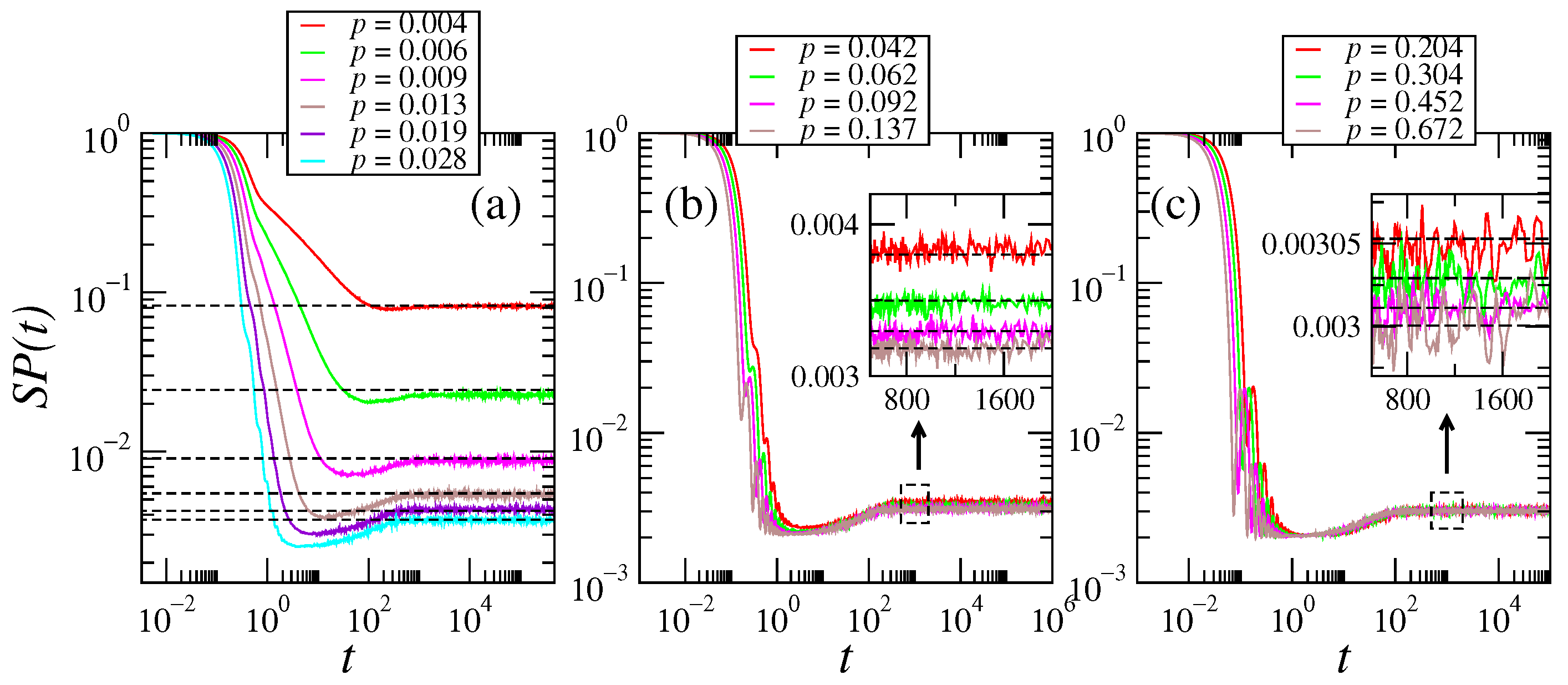
Now, in Figure 2, we present the temporal evolution of the SP for an ensemble of 2 × 10 4 ER random networks of size n = 1000 and several values of the connection probability p. From Figure 2, we clearly observe the different regimes of the SP behavior [25]: The universal exponential initial decay is followed by a slower decay until the SP reaches a minimum value, then it shows a small recovery (ramp) before saturation.
In what follows, we analyze in detail the different regimes in the time evolution of the SP: The decay of the SP (the decay after the exponential initial decay), the correlation hole (the regime between the minimum value of the SP and its saturation value), and the saturation of the SP.

3.1. Decay of the SP

The initial fast decay of the SP can be well described by the dominant term in the power series expansion of the inner product | Ψ ( 0 ) | | Ψ ( t ) | 2 [23],
S P ( t 1 ) 1 σ i n i 2 t 2 ,
where σ i n i corresponds to Equation (6).
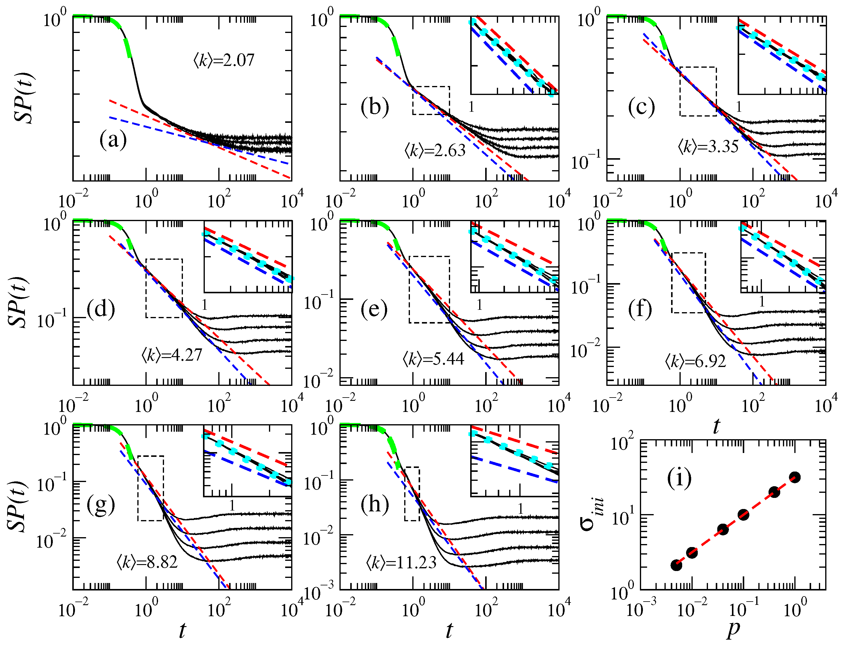
In order to characterize the standard deviation of the energy distribution of the initial state σ i n i in terms of the connection probability p, in Figure 3g, we plot σ i n i for several values of p for networks of size n = 1000 . Here, we find that the σ i n i vs. p curve follows a power-law of the form σ i n i = A p B with fitting values A = 31.68175 1000 1 / 2 and B = 0.5006 1 / 2 . This shows that σ i n i is directly related to the average degree k as σ i n i C n p C k 1 / 2 ( C is a constant with energy units); see Equation (1). This scaling follows heuristically from the spectral properties of the weighted adjacency random matrix model considered here. The off-diagonal entries of the adjacency matrix are independent random variables with mean zero. When an edge is present, the entry is drawn from N ( 0 , 1 ) ; otherwise it is zero. The resulting matrix is thus a diluted Wigner matrix with effective variance p. This is in accordance with the well-known spectral width of Wigner-type random matrices with entry variance p; the bulk of the spectrum is confined to [ 2 n p , 2 n p ] in the limit n [31]. Since the LDOS at a typical node reflects the global spectral density, its standard deviation σ i n i is governed by the same spectral bandwidth, leading to σ i n i n p k 1 / 2 . Thus, in Figure 3a–h, we plot
S P ( t 1 ) 1 C 2 k t 2
(as green dashed lines) and observe a very good correspondence with the SP curves at small times for different values of k . Now, from Figure 2a, when p < p c (here p c = 0 . 11 ¯ ), we observe a clean power-law decay,
S P ( t ) t μ ,
of the SP after the initial fast decay. When p p c , see Figure 2b, oscillations emerge along the decay of the SP. These oscillations increase in amplitude for increasing p, see Figure 2c, approaching the GOE line-shape prediction for the SP [26,27,28].
Indeed, studies of disordered noninteracting systems have shown that the power μ in the power-law decay of the SP, see Equation (9), is directly related to the correlation dimension D 2 of the corresponding eigenstates, i.e., μ D 2 [32,33,34]; see Appendix A. Also, in the study of the dynamics at the many-body localization transition, the correlation dimension associated with the initial state D 2 ˜ has also been related to μ , i.e., μ D 2 ˜ [35,36]; see also Appendix A. Therefore, in what follows, we compute D 2 and D 2 ˜ and compare them with the power μ .
Since we aim to characterize the power-law behavior of the SP curves and the average degree fixes the localization properties of the eigenstates of the network, in Figure 3, we show S P ( t ) plots for different fixed values of k , from k = 2.07 [see panel (a)] to k = 11.23 [see panel (h)] and four network sizes n, increasing from top to bottom. We consider the whole (full) Erdős–Rényi graph, including all nodes, and average over many realizations for each fixed value of k . This is the procedure followed throughout the present work; no selection is made based on connectivity or the giant component. Red dashed and blue dashed lines proportional to t D 2 and t D ˜ 2 , respectively, are shown in Figure 3 to guide the eye. From Figure 3a, we note that neither t D 2 nor t D ˜ 2 matches the decay of S P ( t ) . However, as k increases, t D 2 coincides with the decay of S P ( t ) at short times, as we can see in the insets of Figure 3b–d, where the best fit t μ is shown as dotted cyan lines and t D 2 and t D 2 ˜ are shown in dashed lines to guide the eye. Notably, t D ˜ 2 agrees better with the decay of S P ( t ) when k = 4.27 , 5.44 and 6.92 (see insets in Figure 3d–f and Table 1). Then, we conclude that t D 2 better predicts the decay of S P ( t ) for small values of k , see Figure 3b,c, while t D ˜ 2 works better for large values of k , see Figure 3d–f. For k > 6.92 , see Figure 3g,h, neither t D 2 nor t D ˜ 2 match the decay of S P ( t ) . Therefore, we can also conclude that the interval of k where the decay of S P ( t ) can be predicted by t D 2 or t D ˜ 2 is very narrow.
On the other hand, the time-averaged survival probability, also known as the temporal autocorrelation function [33], has been used extensively to analyze the dynamics of disordered systems at the mobility edge [33,34,37]. More recently, it has been applied to the study of the many-body localization transition in the 1D Heisenberg model [35]. In fact, it has been observed that the dimension D 2 ˜ directly governs the decay of the time-averaged survival probability, which follows a power-law proportional to t D 2 ˜ . Due to its relevance, the analysis of this quantity seems pertinent for our study.
The time-averaged survival probability is defined as:
C ( t ) = 1 t 0 t S P ( τ ) d τ .
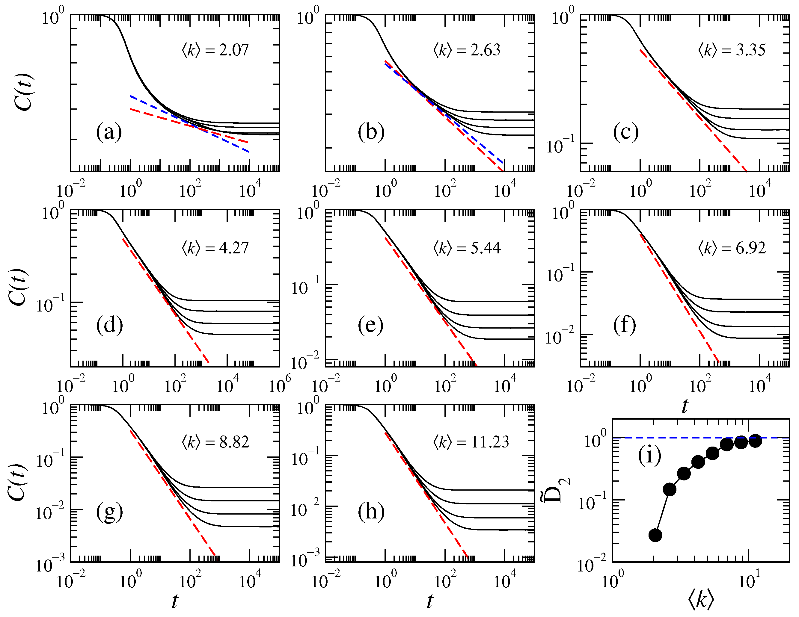
Thus, in Figure 4a–h, we present C ( t ) for the same values of the average degree k and network sizes n reported in Figure 3. In every panel, we also plot t D 2 ˜ as red dashed lines, illustrating that the decay of C ( t ) is well described by this power-law. Notably, the best agreement between C ( t ) and t D 2 ˜ is observed when k 3.35 . Additionally, for comparison purposes, in Figure 4a,b, we also include t D 2 as blue dashed lines. As already observed in Figure 3a,b, t D 2 is a good indicator of the S P ( t ) decay; interestingly, it also proves to be a good descriptor for C ( t ) in the same parameter regime.
Finally, for completeness, in Figure 4g, we present the generalized dimension D ˜ 2 vs. k . This plot illustrates the asymptotic transition to D ˜ 2 = 1 (horizontal blue dashed line) as k increases. We note that the crossover to GOE-like behavior ( D ˜ 2 1 ) occurs at k 10 , which is larger than the connectivity threshold k ln ( n ) [ 5.5 , 7.6 ] for the system sizes studied here. We also note the crossover behavior in the analysis of the relative depth of the correlation hole; see the next section.

3.2. Correlation Hole

From Figure 2, note that the decay of the S P ( t ) persists until it reaches its minimum value at a time which is known as the Thouless time, t T h ; see, e.g., [24]. Indeed, the minimum value of the S P ( t ) is also the bottom of the correlation hole.
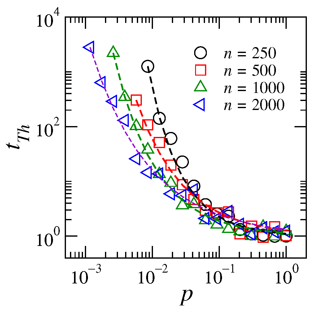
Then, in Figure 5, we report t T h of ER random networks of size n as a function of p. We observe that for a given value of p, the larger the network size the smaller the Thouless time. Also, for a given n, we observe the exponential decay of t T h with p which is empirically described by
t T h e A p B ,
where A and B are fitting constants; see the dashed lines in Figure 5.
Figure 5. Thouless time t T h of ER random networks of size n as a function of the connection probability p. Dashed lines correspond to fittings of Equation (11) to the data with fitting parameters reported in Table 2.
Complexities 02 00017 g005
Table 2. Values of the parameters A and B in Equation (11) as extracted from fittings to the curves t T h vs. p of Figure 5.
t Th
nAB
2500.1050.886
5000.2390.615
10000.1310.685
20000.2870.492
Additionally, the relative depth of the correlation hole has been used to detect the integrability-to-chaos transition in disordered systems and more recently to detect the many-body localization phase in disordered interacting systems [38]. Therefore, the study of this quantity is relevant to our study.
The relative depth of the correlation holes is defined as
η = S P ¯ S P m i n S P ¯ .
Here, S P ¯ is the saturation value of the S P ( t ) , and S P m i n is the minimum value of the S P ( t ) . In the case of the GOE, S P ¯ 3 / n and S P m i n 2 / n . Then, we expect to observe a transtion from η 0 when p 0 to η 1 / 3 when p 1 .
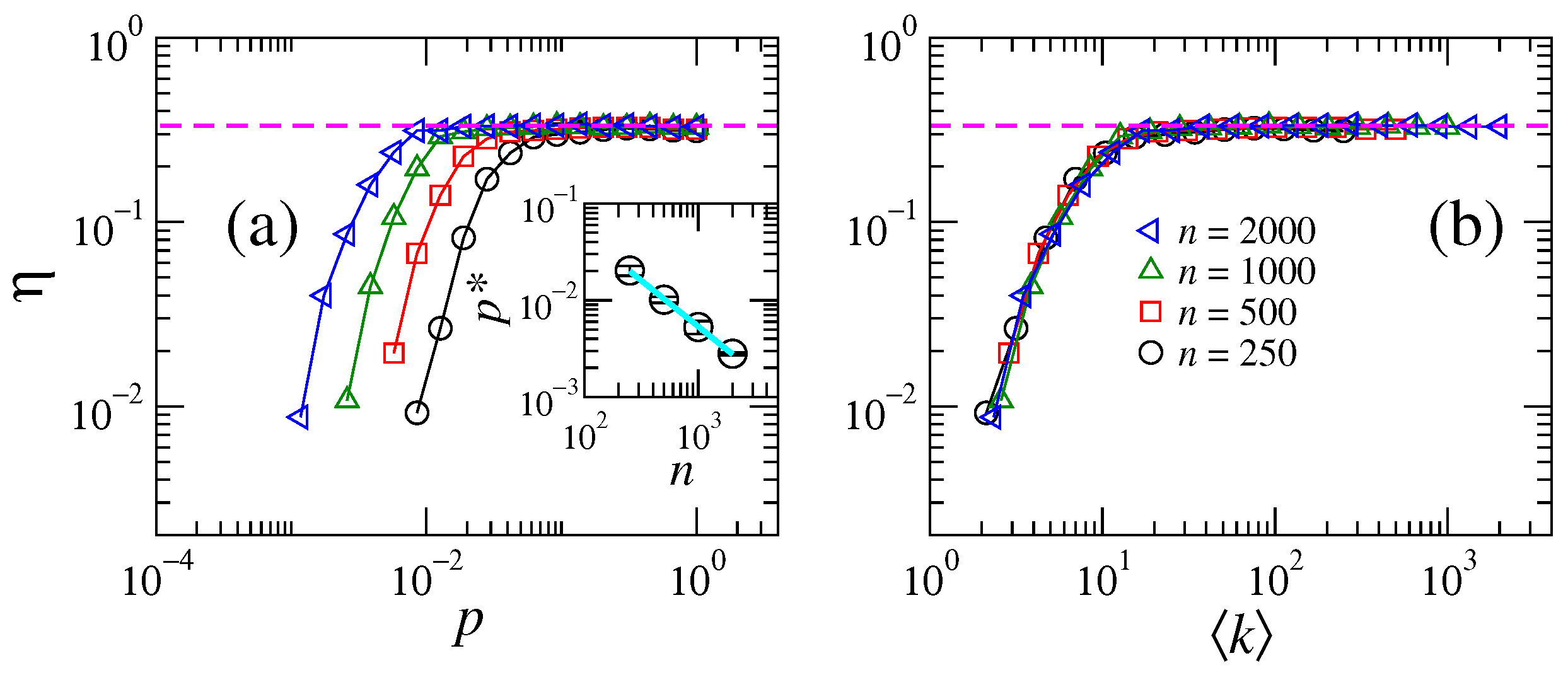
Thus, in Figure 6a, we present η for ER random networks as a function of p. From this figure, we observe, as expected, that η approaches 1/3 for increasing p. Moreover, the larger the network size n, the smaller the value of p needed for η to approach the GOE regime; that is, the curves η vs. p are displaced to the left in the p-axis for increasing n. Now, when we plot η as a function of k , see Figure 4b, all the curves fall one on top of the other. This observation suggests that the average degree k is the relevant scaling parameter for η . To test this hypothesis, we perform a finite-size scaling analysis of η . We characterize the position of the η vs. p curves along the p-axis by the value p * at which η = 0.1 . As shown in the inset of Figure 6a, the data for p * vs. n are well described by a power-law p * = A n B , yielding A = 3.8028 and B = 0.9507 ± 0.0133 , which is approximately 1. This confirms the expected inverse scaling with system size. Consequently, as k * p * n , k * must be constant, thus confirming k as the scaling parameter of η .
This verification is in agreement with previous studies where it has been shown that k scales the topological [39], spectral [16], and transport [40] properties of ER random networks. For the finite sizes and parameter range studied here, the relative depth of the correlation hole η exhibits a crossover toward its GOE value around k 10 [16], where the GOE limit is depicted by the magenta dashed line at η = 1 / 3 . This empirical crossover should not be interpreted as a universal delocalization threshold.

3.3. Saturation Value of the SP

We also note from Figure 2a that the saturation values of the S P ( t ) are smaller the larger p is, while the S P ( t ) reaches its saturation value faster for increasing p. Also, as the networks become more connected, the saturation values of the S P ( t ) approach the GOE prediction of 3 / n ; see the insets in Figure 2b,c.
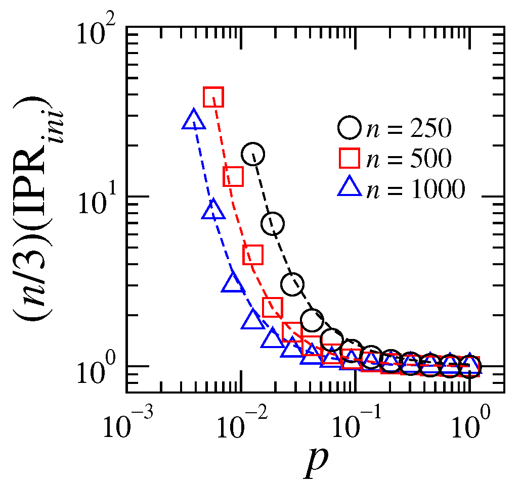
In Figure 7, we plot the inverse participation ratio of the initial state IPR i n i (divided by 3 / n , the GOE saturation value) as a function of p for three different network sizes: n = 250 , 500, and 1000 (represented by different colors). Since the IPR i n i is the saturation value of the S P ( t ) , the ratio IPR i n i / ( 3 / n ) approaches 1 as p 1 , as shown in Figure 7. Interestingly, we found that the decay of IPR i n i / ( 3 / n ) is dictated by the heuristic expression:
IPR i n i 3 n e A p B ,
where A and B are fitting constants. Indeed, the dashed lines in Figure 7 correspond to fittings of Equation (13) to the data with the fitting constants reported in Table 3.

4. Conclusions

In this work, within a random matrix theory (RMT) approach, we analyzed the survival probability S P ( t ) of Erdös–Renyi (ER) random networks in the crossover from isolated nodes to fully connected networks. Note that the crossover from isolated nodes to fully connected networks corresponds to the crossover from localized to extended eigenstates of the corresponding randomly weighted adjacency matrices. We recall that the ER model is defined as n nodes connected randomly with probability p.
We observed that the time evolution of the SP of a delta-like excitation in ER random networks shows the standard panorama reported for RMT models: The SP displays an initial fast decay followed by a power-law decay, then it reaches a minimum value (at a time which is known as the Thouless time t T h ) before saturation; see Figure 2.
For the fast decay of the SP, we were able to write down an expression that depends on the average degree k n p only, see Equation (8). Also, we observed that once k is fixed, the curves of S P ( t ) , as well as its time-average C ( t ) , coincide for different network sizes in the power-law decay regime; see Figure 3 and Figure 4. Moreover, we showed that in a short time window and for intermediate values of k (specifically, k 2.63 , 3.35), the power-law decay of S P ( t ) is well approximated by t D 2 and t D ˜ 2 (specifically, k 4.27 , 5.44, 6.92) while for C ( t ) , the decay is dictated by t D ˜ 2 . Here, D 2 and D ˜ 2 are the correlation dimension of the eigenstates of the ER random networks and the correlation dimension associated with the initial state, respectively. However, we emphasize that this agreement is only approximate and depends on k , becoming less accurate for larger k or longer times.
In addition, we showed that the relative depth of the correlation hole of the SP scales with k (see Figure 6), while both, t T h and the IPR of the initial state, decay exponentially with p; see Figure 5 and Figure 7. Finally, we provided strong evidence of multifractality of the eigenstates of the randomly weighted adjacency matrices of ER networks; see Figure A1 and Figure A2.
Furthermore, we note that the present framework for studying the SP on ER networks with undirected (bidirectional) edges could be naturally extended to oriented random graphs. In particular, the spectral properties of randomly oriented graphs, as studied via the skew-adjacency matrix formalism in ref. [41] and via the magnetic adjacency matrix in refs. [15,18], provide a promising route for analyzing transport and SP in directed ER networks. While a thorough investigation of such directed systems lies beyond the scope of this work, we believe that the combination of the survival probability approach developed here with the spectral theory of oriented random graphs could yield interesting insights into how edge directionality affects the spectral properties and quantum dynamics in complex networks. We hope that our study may motivate further research on the application of RMT techniques to the study of dynamical properties of random network models.

Author Contributions

Conceptualization, K.P.-M. and J.A.M.-B.; methodology, K.P.-M. and J.A.M.-B.; software, K.P.-M.; validation, K.P.-M. and J.A.M.-B.; formal analysis, K.P.-M. and J.A.M.-B.; investigation, K.P.-M.; resources, K.P.-M. and J.A.M.-B.; data curation, K.P.-M.; writing—original draft preparation, K.P.-M.; writing—review and editing, K.P.-M. and J.A.M.-B.; visualization, K.P.-M.; supervision, K.P.-M. and J.A.M.-B.; project administration, K.P.-M. and J.A.M.-B.; funding acquisition, J.A.M.-B. All authors have read and agreed to the published version of the manuscript.

Funding

This research was funded by SECIHTI, Grant No. CBF-2025-I-2236, Mexico (J.A.M.-B.). K.P.-M. thanks support from SECIHTI (Postdoctoral Fellowship CVU 1008060), Mexico.

Institutional Review Board Statement

Not applicable.

Informed Consent Statement

Not applicable.

Data Availability Statement

The original contributions presented in this study are publicly available in a GitHub repository. The data and code are released under a MIT license and can be accessed at the following URL: https://github.com/Kevin-Peralta-Martinez/complex_systems/tree/main/SP_ER (accessed on 24 April 2026).

Acknowledgments

The authors thank Lea F. Santos for valuable discussions and feedback on an early draft of this manuscript.

Conflicts of Interest

The authors declare no conflicts of interest.

Abbreviations

The following abbreviations are used in this manuscript:
CTQWContinuous time quantum walk
ERErdös–Renyi
SPSurvival probability
RMTRandom matrix theory
RGGsRandom geometric graphs
PEPoisson ensemble
GOEGaussian orthogonal ensemble
LDOSLocal density of states
PBRMPower-law random banded matrix

Appendix A. Multifractal Dimensions of Eigenstates
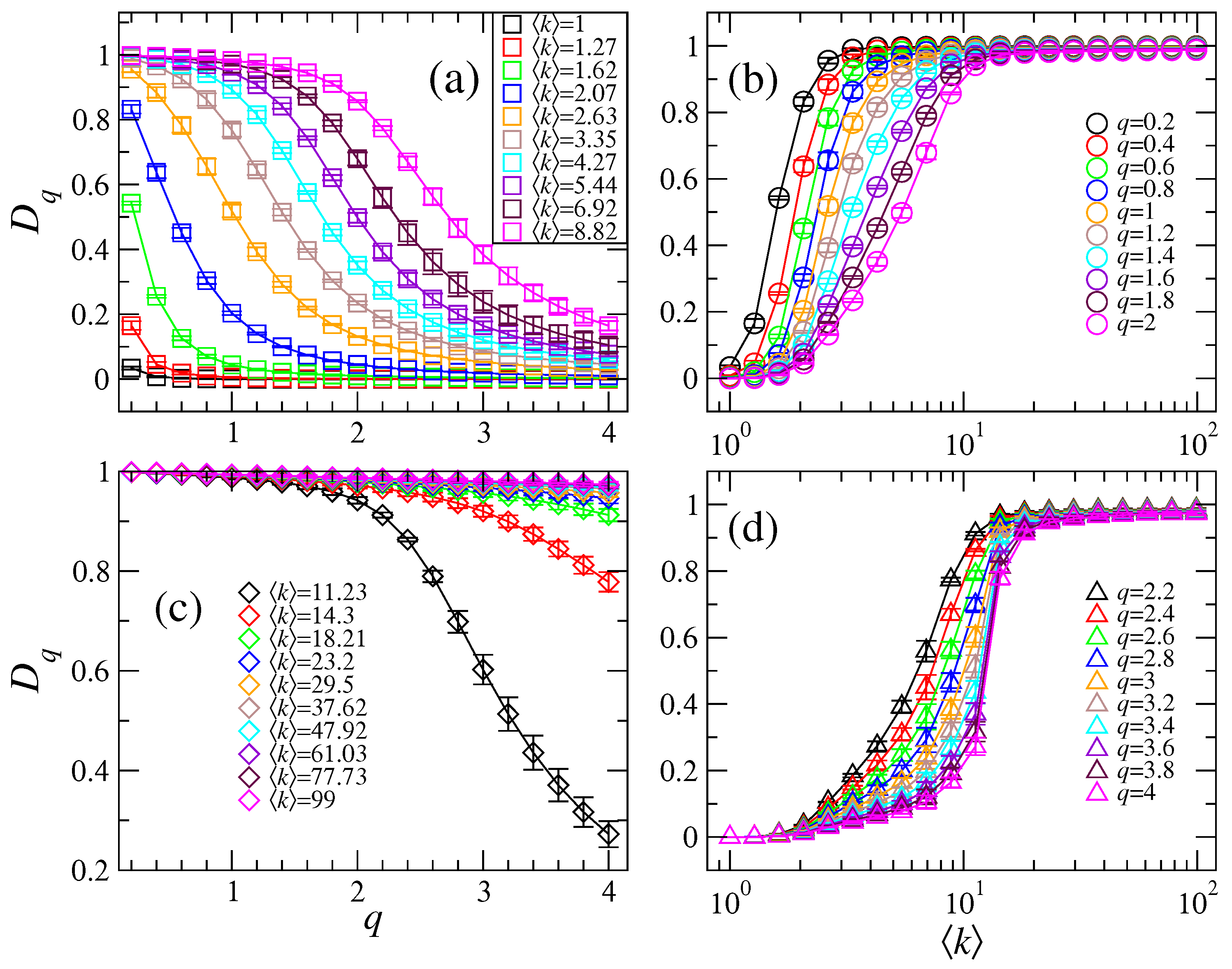
In Section 3.1, we have shown that the decay of the survival probability S P ( t ) and that of the time-averaged survival probability C ( t ) of ER random networks are governed by the power-laws t D 2 and t D ˜ 2 , respectively. Here, D 2 is the correlation dimension of the eigenstates of the adjacency matrix of the ER random networks while D ˜ 2 is the correlation dimension of the initial state. Thus, in this Appendix A, we give details of the calculation of D 2 and D ˜ 2 but we also report the generalized dimensions D q .
Disordered systems that manifest the Anderson transition, a metal-to-insulator transition driven by the disorder amplitude, exhibit a number of critical properties. One well-established signature of the Anderson transition is that the eigenstates of the corresponding disordered systems are multifractal objects at and in a small neighborhood of the critical transition point [42]. Lattice models, such as the 3D Anderson tight-binding model, the power-law random banded matrix (PRBM) model, and critical random matrix ensembles, have been extensively used to study the Anderson transition [42,43,44]. In addition, multifractal eigenstates at the critical point have been reported for random graph models [45] as well as for a diluted version of the PRBM [46] which represents ER-like random networks with long-range interactions.
The multifractality of the eigenstates Ψ α is characterized by the generalized dimension D q , which is computed from the size scaling of the average inverse participation ratio as [43,47]
IPR ( q ) i = 1 n Ψ i α 2 q α n ( q 1 ) D q , q 1 .
While the information dimension D 1 is computed from the size scaling of the average Shanon entropy
S i = 1 n Ψ i α 2 ln Ψ i α 2 α D 1 ln n .
When computing D q for the eigenstates of a disordered system, D q = d and D q = 0 correspond to fully delocalized states and localized states, respectively. Here, d is the embedding dimension of the system. While 0 < D q < d indicates multifractal states, meaning that such states do not extend over the entire available configuration space.
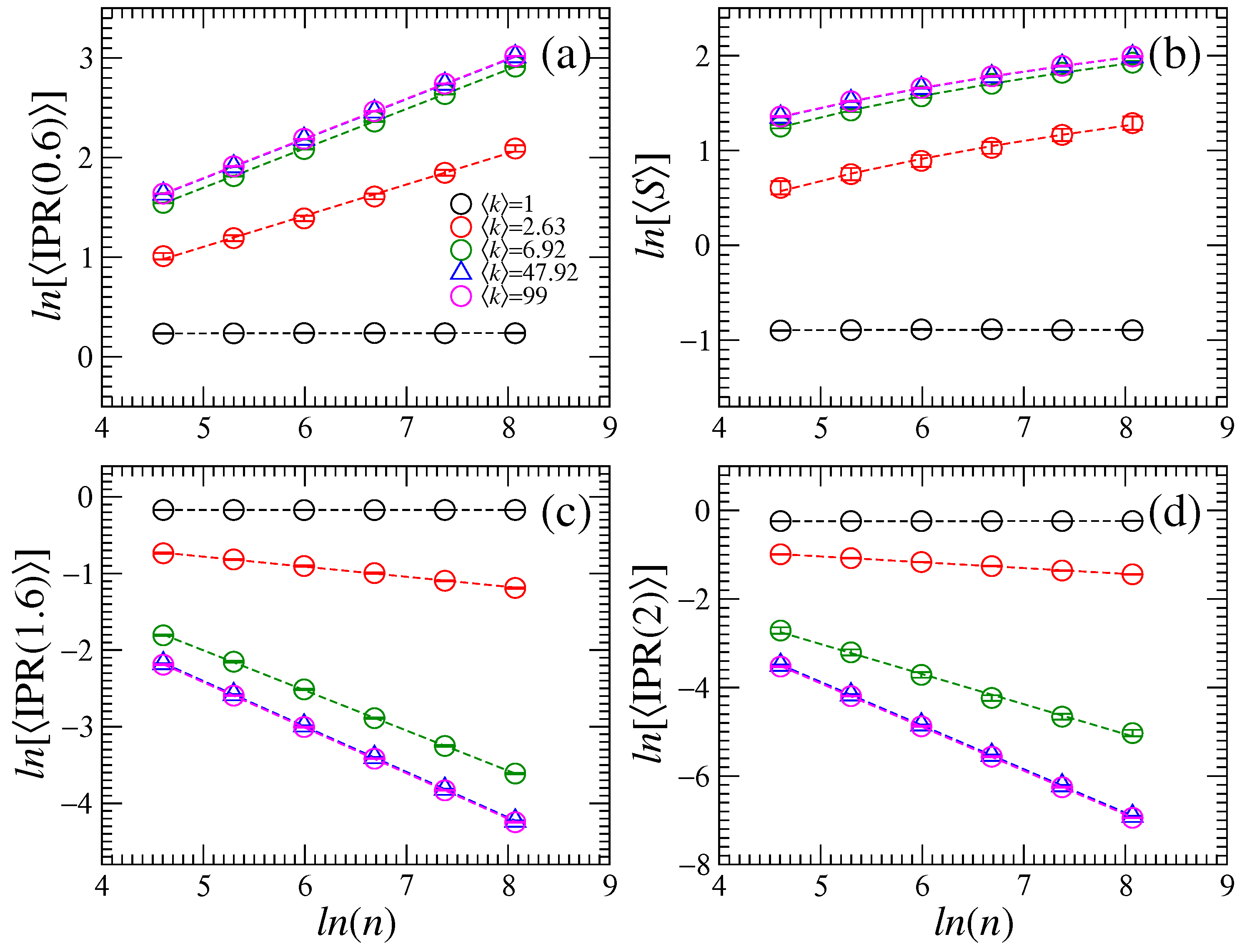
Figure A1. Average inverse participation ratio IPR ( q ) of ER random networks as a function of the size n for (a) q = 0.6 , (c) q = 1.6 , and (d) q = 2 . In panel (b), the average Shannon entropy S of ER random networks as a function of n is shown. Several values of the average degree k are reported in each panel, as indicated in panel (a). The averages are taken over 20 % of the eigenstates at the center of the band and over 10 6 / ( 0.2 n ) random network realizations.
Complexities 02 00017 g0a1
Figure A2. Multifractal dimensions D q of ER random networks as a function of (a,c) q and (b,d) k for several values of k and q, respectively. Error bars are shown for each case (most of them are smaller than symbol size).
Complexities 02 00017 g0a2
Here, since we deal with ER random networks represented by randomly weighted adjacency matrices which are members of a diluted GOE that interpolates between the Poisson ensemble when p 0 and the GOE when p 1 , we expect to observe a transition from D q = 0 to D q = 1 when increasing k from k 0 to k n 1 .
In Figure A1, we present the IPR ( q ) of ER random networks as a function of n, in log-log scale, for q = 0.6 , 1, and 2; as well as S vs. n. In each panel, we show curves for different values of k . From Figure A1, we observe that the slopes (in log-log scale) of the curves of IPR ( q ) vs. n and of S vs. n, which coincide with D q and D 1 , respectively, are approximately zero for small k while they approach one for large k . This indicates a transition from an insulating regime (localized eigenstates) to a metallic regime (extended eigenstates) by increasing k . Remarkably, the slopes between zero and one of the curves IPR ( q ) vs. n and S vs. n, observed in Figure A1 for intermediate values of k , indicate the existence of multifractal eigenstates.
Then, in Figure A2, we present D q of ER random networks as a function of q (see left panels) and also as a function of k (see right panels). The values of D q reported in Figure A2 are obtained from fittings of the data IPR ( q ) vs. n and S vs. n with Equations (A1) and (A2), respectively.
From Figure A2, we note a clear multifractal behavior for the eigenstates of the weighted adjacency matrices of ER random networks: D q D q for q q . This is in accordance with predictions of ref. [48], where a multifractal phase was identified for sparse weighted ER graphs. Also, we clearly observe the delocalization-to-localization transition as a function of k : D q 1 for large k and D q 0 for small k .
Finally, we mention that we computed D ˜ 2 from the scaling of the inverse participation ratio of the initial state, that is [35]
IPR ( 2 ) i n i = β C i n i β 4 n D ˜ 2 .
In our analysis, we computed IPR ( 2 ) i n i for networks of sizes n = 100 , 200, 400, 800, 1600, and 3200 over an eigenstate window of 20 % of the matrix size around | ϕ i n i .

References

  1. Moreno, Y.; Nekovee, M.; Pacheco, A.F. Dynamics of rumor spreading in complex networks. Phys. Rev. E 2004, 69, 066130. [Google Scholar] [CrossRef] [Scilit] [PubMed]
  2. Margiotta, R.G.; Kühn, R.; Sollich, P. Glassy dynamics on networks: Local spectra and return probabilities. J. Stat. Mech. 2019, 093304. [Google Scholar] [CrossRef] [Scilit]
  3. Chelminiak, P. Return probability for random walks on scale-free complex trees. Phys. Lett. 2011, 375, 3114–3118. [Google Scholar] [CrossRef] [Scilit]
  4. Riascos, A.P.; Mateos, J.L. Random walks on weighted networks: Exploring local and non-local navigation strategies. arXiv 2019, arXiv:1901.05609. [Google Scholar]
  5. Estrada, E. d-Path Laplacians and Quantum Transport on Graphs. Mathematics 2020, 8, 527. [Google Scholar] [CrossRef] [Scilit]
  6. Riascos, A.P.; Mateos, J.L. Fractional dynamics on networks: Emergence of anomalous diffusion and Lévy flights. Phys. Rev. E 2014, 90, 032809. [Google Scholar] [CrossRef] [Scilit] [PubMed]
  7. Riascos, A.P.; Mateos, J.L. Fractional quantum mechanics on networks: Long-range dynamics and quantum transport. Phys. Rev. E 2015, 92, 052814. [Google Scholar] [CrossRef] [Scilit] [PubMed]
  8. Mülken, O.; Blumen, A. Continuous-time quantum walks: Models for coherent transport on complex networks. Phys. Rep. 2011, 502, 37–87. [Google Scholar] [CrossRef] [Scilit]
  9. Mülken, O.; Blumen, A. Efficiency of quantum and classical transport on graphs. Phys. Rev. E 2006, 73, 066117. [Google Scholar] [CrossRef] [Scilit] [PubMed]
  10. Anishchenko, A.; Blumen, A.; Mülken, O. Enhancing the spreading of quantum walks on star graphs by additional bonds. Quantum Inf. Process. 2012, 11, 1273–1286. [Google Scholar] [CrossRef] [Scilit]
  11. Agliari, E. Trapping of continuous-time quantum walks on Erdös–Rényi graphs. Phys. A Stat. Mech. Appl. 2011, 390, 1853–1860. [Google Scholar] [CrossRef] [Scilit]
  12. Xu, X.P.; Liu, F. Continuous-time quantum walks on Erdös–Rényi networks. Phys. Lett. A 2008, 372, 6727–6732. [Google Scholar] [CrossRef] [Scilit]
  13. Solomonoff, R.; Rapoport, A. Connectivity of random nets. Bull. Math. Biophys. 1951, 13, 107. [Google Scholar] [CrossRef] [Scilit]
  14. Rényi, A.; Erdos, P. On random graphs. Publ. Math. 1959, 6, 290–297. [Google Scholar]
  15. Peron, T.; de Resende, B.M.F.; Rodrigues, F.A.; Costa, L.d.F.; Mendez-Bermudez, J.A. Spacing ratio characterization of the spectra of directed random networks. Phys. Rev. E. 2020, 102, 062305. [Google Scholar] [CrossRef] [Scilit] [PubMed]
  16. Mendez-Bermudez, J.A.; Alcazar-López, A.; Martínez-Mendoza, A.J.; Rodrigues, F.A.; Peron, T.K.D.M. Universality in the spectral and eigenfunction properties of random networks. Phys. Rev. E 2015, 91, 032122. [Google Scholar] [CrossRef] [Scilit] [PubMed]
  17. Alonso, L.; Mendez-Bermudez, J.A.; Gonzalez-Melendrez, A.; Moreno, Y. Weighted random-geometric and random-rectangular graphs: Spectral and eigenfunction properties of the adjacency matrix. J. Complex Netw. 2018, 6, 753. [Google Scholar]
  18. Peralta-Martinez, K.; Mendez-Bermudez, J.A. Directed random geometric graphs: Structural and spectral properties. J. Phys. Complex. 2023, 4, 015002. [Google Scholar]
  19. Erdös, L.; Knowles, A.; Yau, H.-T.; Yin, J. Spectral statistics of Erdős–Rényi graphs I: Local semicircle law. Ann. Probab. 2013, 41, 2279–2375. [Google Scholar] [CrossRef] [Scilit]
  20. Erdös, L.; Knowles, A.; Yau, H.; Yin, J. Spectral statistics of Erdős-Rényi Graphs II: Eigenvalue spacing and the extreme eigenvalues. Commun. Math. Phys. 2012, 314, 587–640. [Google Scholar] [CrossRef] [Scilit]
  21. Rodgers, G.J.; Bray, A.J. Density of states of a sparse random matrix. Phys. Rev. B 1988, 37, 3557. [Google Scholar] [CrossRef] [Scilit] [PubMed]
  22. Anderson, P.W. Absence of diffusion in certain random lattices. Phys. Rev. 1958, 109, 1492–1505. [Google Scholar] [CrossRef] [Scilit]
  23. Torres-Herrera, E.J.; Karp, J.; Távora, M.; Santos, L.F. Realistic many-body quantum systems vs. full random matrices: Static and dynamical properties. Entropy 2016, 18, 359. [Google Scholar] [CrossRef] [Scilit]
  24. Schiulaz, M.; Torres-Herrera, E.J.; Santos, L.F. Thouless and relaxation time scales in many-body quantum systems. Phys. Rev. B 2019, 99, 174313. [Google Scholar] [CrossRef] [Scilit]
  25. Zarate-Herrada, D.A.; Santos, L.F.; Torres-Herrera, E.J. Generalized survival probability. Entropy 2023, 25, 205. [Google Scholar] [CrossRef] [Scilit] [PubMed]
  26. Távora, M.; Torres-Herrera, E.J.; Santos, L.F. Inevitable power-law behavior of isolated many-body quantum systems and how it anticipates thermalization. Phys. Rev. A 2016, 94, 041603. [Google Scholar] [CrossRef] [Scilit]
  27. Távora, M.; Torres-Herrera, E.J.; Santos, L.F. Power-law decay exponents: A dynamical criterion for predicting thermalization. Phys. Rev. A 2017, 95, 013604. [Google Scholar] [CrossRef] [Scilit]
  28. Torres-Herrera, E.J.; Kollmar, D.; Santos, L.F. Relaxation and thermalization of isolated many-body quantum systems. Phys. Scr. 2015, T165, 014018. [Google Scholar] [CrossRef] [Scilit]
  29. Izrailev, F.M.; Castaneda-Mendoza, A. Return probability: Exponential versus Gaussian decay. Phys. Lett. A 2006, 350, 355–362. [Google Scholar] [CrossRef] [Scilit]
  30. Kravtsov, V.E.; Ossipov, A.; Yevtushenko, O.M. Return probability and scaling exponents in the critical random matrix ensemble. J. Phys. A Math. Theor. 2011, 44, 305003. [Google Scholar] [CrossRef] [Scilit]
  31. Wigner, E.P. On the distribution of the roots of certain symmetric matrices. Ann. Math. 1958, 67, 325–327. [Google Scholar] [CrossRef] [Scilit]
  32. Huckestein, B.; Klesse, R. Wave-packet dynamics at the mobility edge in two-and three-dimensional systems. Phys. Rev. B 1999, 59, 9714. [Google Scholar] [CrossRef] [Scilit]
  33. Ketzmerick, R.; Petschel, G.; Geisel, T. Slow decay of temporal correlations in quantum systems with Cantor spectra. Phys. Rev. Lett. 1992, 69, 695. [Google Scholar] [CrossRef] [Scilit] [PubMed]
  34. Huckstein, B.; Schweitzer, L. Relation between the correlation dimensions of multifractal wave functions and spectral measures in integer quantum Hall systems. Phys. Rev. Lett. 1994, 72, 713. [Google Scholar] [CrossRef] [Scilit] [PubMed]
  35. Torres-Herrera, E.J.; Santos, L.F. Dynamics at the many-body localization transition. Phys. Rev. B 2015, 92, 014208. [Google Scholar] [CrossRef] [Scilit]
  36. Zarate-Herrada, D.A.; Vallejo-Fabila, I.; Santos, L.F.; Torres-Herrera, E.J. Dynamical detection of extended nonergodic states in many-body quantum systems. arXiv 2025, arXiv:2505.23910. [Google Scholar]
  37. Seng Ng, G.; Bodyfelt, J.; Kottos, T. Critical fidelity at the metal-insulator transition. Phys. Rev. Lett. 2006, 97, 256404. [Google Scholar] [CrossRef] [Scilit] [PubMed]
  38. Torres-Herrera, E.J.; Santos, L.F. Dynamical manifestations of quantum chaos: Correlation hole and bulge. Phil. Trans. R. Soc. A 2017, 375, 20160434. [Google Scholar] [CrossRef] [Scilit] [PubMed]
  39. Aguilar-Sanchez, R.; Herrera-Gonzalez, I.F.; Mendez-Bermudez, J.A.; Sigarreta, J.M. Computational properties of general indices on random networks. Symmetry 2020, 12, 1341. [Google Scholar] [CrossRef] [Scilit]
  40. Martinez-Mendoza, A.J.; Alcazar-Lopez, A.; Mendez-Bermudez, J.A. Scattering and transport properties of tight-binding random networks. Phys. Rev. E 2013, 88, 122126. [Google Scholar] [CrossRef] [Scilit] [PubMed]
  41. Shang, Y. On the skew-spectral distribution of randomly oriented graphs. Ars. Comb. 2018, 140, 63–71. [Google Scholar]
  42. Evers, F.; Mirlin, A.D. Anderson transitions. Rev. Mod. Phys. 2008, 80, 1355. [Google Scholar] [CrossRef] [Scilit]
  43. Mendez-Bermudez, J.A.; Alcazar-Lopez, A.; Varga, I. Multifractal dimensions for critical random matrix ensembles. EPL 2012, 98, 37006. [Google Scholar] [CrossRef] [Scilit]
  44. Mirlin, A.D.; Fyodorov, Y.V.; Dittes, F.M.; Quezada, J.; Seligman, T.H. Transition from localized to extended eigenstates in the ensemble of power-law random banded matrices. Phys. Rev. E 1996, 54, 3221. [Google Scholar] [CrossRef] [Scilit] [PubMed]
  45. García-Mata, I.; Giraud, O.; Georgeot, B.; Martin, J.; Dubertrand, R.; Lemarié, G. Scaling theory of the Anderson transition in random graphs: Ergodicity and universality. Phys. Rev. Lett. 2017, 118, 166801. [Google Scholar] [CrossRef] [Scilit] [PubMed]
  46. Vega-Oliveros, D.A.; Mendez-Bermudez, J.A.; Rodrigues, F.A. Multifractality in random networks with power-law decaying bond strengths. Phys. Rev. E 2019, 99, 042303. [Google Scholar] [CrossRef] [Scilit] [PubMed]
  47. Bogomolny, E.; Giraud, O. Multifractal dimensions for all moments for certain critical random-matrix ensembles in the strong multifractality regime. Phys. Rev. E 2012, 85, 046208. [Google Scholar] [CrossRef] [Scilit] [PubMed]
  48. Baron, J.W.; Rogers, T. Local density of states distribution and multifractal eigenvectors of weighted random networks via the cavity approach. arXiv 2026, arXiv:2606.10915. [Google Scholar]
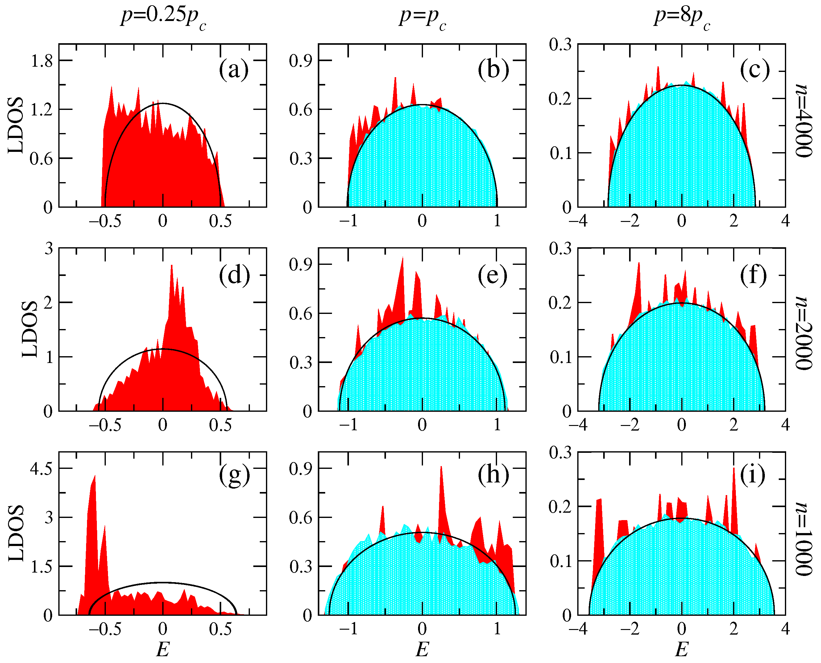
Figure 1. Histograms of the local density of states (LDOS) at the center of the band of ER random networks. Several combinations of sizes n (different rows) and connection probabilities p (different columns) are considered. Specifically, (a,d,g) p = 0.25 p c , (b,e,h) p = p c , and (c,f,i) p = 8 p c with p c = n 2 / 3 / ( n 1 ) . Each red histogram is constructed from a single random network realization, whereas each blue histogram is constructed from 50 random network realizations. Black lines are the semicircles of Equation (5) with σ i n i given by Equation (6).
Complexities 02 00017 g001
Figure 2. (ac) Survival probability S P ( t ) of ER random networks of size n = 1000 and several values of the connection probability p. Insets in panels (b,c) are enlargements of the corresponding dashed squares. Horizontal dashed black lines indicate the saturation value of the curves. The connection probability p increases from top to bottom.
Complexities 02 00017 g002
Figure 3. (ah) Survival probability S P ( t ) of ER random networks for several values of the average degree k , as indicated in the panels. Four graph sizes are reported in each panel ( n = 250 , 500, 1000, 2000), increasing from top to bottom. Red dashed lines correspond to t D 2 with (a) D 2 = 0.0446 , (b) D 2 = 0.1316 , (c) D 2 = 0.234 , (d) D 2 = 0.3509 , (e) D 2 = 0.4976 , (f) D 2 = 0.6868 , (g) D 2 = 0.8615 , and (h) D 2 = 0.9477 . Blue dashed lines correspond to t D ˜ 2 with (a) D ˜ 2 = 0.0269 , (b) D ˜ 2 = 0.1467 , (c) D ˜ 2 = 0.2647 , (d) D ˜ 2 = 0.4062 , (e) D ˜ 2 = 0.5589 , (f) D ˜ 2 = 0.7786 , (g) D ˜ 2 = 0.8398 , and (h) D ˜ 2 = 0.8873 . Green dashed lines correspond to 1 C 2 k t 2 ; i.e., the decay at very short times. Insets in panels (bh) show a zoom-in of the curves at different t intervals: [ 1 , 10 ] in (bd), [ 0.8 , 9 ] in (e), [ 0.6 , 5 ] in (f), [ 0.6 , 3 ] in (g), and [ 0.6 , 1.5 ] in (h). The best fit to the data is shown as cyan dotted lines t μ , t D 2 is represented by a red dashed line, and t D 2 ˜ by a blue dashed line to guide the eye. A comparison of the fits is shown in Table 1. (i) Standard deviation of the energy distribution of the initial state σ i n i (Equation (6)) as a function of the connection probability p for ER random networks of size n = 1000 . The red dashed line is a power-law fit of the form σ i n i = A p B to the data, with A = 31.682 and B = 0.501 .
Complexities 02 00017 g003
Figure 4. (ah) Time-averaged survival probability C ( t ) of ER random networks for several values of the average degree k , as indicated in the panels. Four graph sizes are reported in each panel ( n = 250 , 500, 1000, 2000); they increase from top to bottom. Red dashed lines correspond to t D 2 ˜ . In panel (a), the blue dashed line corresponds to t D 2 and is plotted for comparison purposes. (i) Generalized dimension D ˜ 2 of the initial state | ϕ i n i as a function of the average degree k . The blue dashed line indicates D 2 ˜ = 1 .
Complexities 02 00017 g004
Figure 6. Relative depth of the correlation hole η of the survival probability S P ( t ) for ER random networks as a function of (a) the connection probability p and (b) the average degree k . Horizontal magenta dashed lines correspond to η = 1 / 3 , the GOE limit. Inset in (a) shows the curves of p * vs. n. Cyan line shows the best power-law fit to data of the form p * = A n B , with A = 3.8028 and B = 0.9507 ± 0.0133 ; symbols are shown with error bars from the fit (smaller than the symbol size).
Complexities 02 00017 g006
Figure 7. Inverse participation ratio of the initial state IPR i n i (divided by 3 / n ) as a function of the connection probability p. Dashed lines are fittings of Equation (13) to the data with fitting parameters reported in Table 3.
Complexities 02 00017 g007
Table 1. Values of μ obtained from the fits to Equation (9) of the S P curves in Figure 3b–h (corresponding to average degrees k ranging from 2.63 to 11.23) are compared with the correlation dimension D 2 and the correlation dimension of the initial state D 2 ˜ . The root mean squared error (RMSE) is shown as a fit-quality metric between the ln ( S P ( t ) ) and D 2 ln ( t ) [ D ˜ 2 ln ( t ) ].
k μ σ μ D2RMSE (D2) D 2 ˜ RMSE ( D 2 ˜ )
2.630.1315 3.45 × 10 4 0.1316 1.8 × 10 3 0.1467 5.45 × 10 3
3.350.2375 3.42 × 10 4 0.234 1.18 × 10 3 0.2647 5.2 × 10 3
4.270.401 9.56 × 10 4 0.3509 6.15 × 10 3 0.4062 2.54 × 10 3
5.440.5723 5.6 × 10 4 0.4976 5.68 × 10 3 0.5589 0.64 × 10 3
6.920.79 0.383 × 10 4 0.6868 8.68 × 10 3 0.7786 2.93 × 10 3
8.821.1526 3.4 × 10 3 0.8615 1.02 × 10 2 0.8398 1.1 × 10 2
11.231.2733 7.91 × 10 3 0.9477 0.96 × 10 2 0.8873 1.08 × 10 2
Table 3. Values of the parameters A and B in Equation (13) as extracted from fittings to the curves IPR ini vs. p of Figure 7.
IPR ini
nAB
2500.024081.096
5000.004751.287
10000.003681.224
Disclaimer/Publisher’s Note: The statements, opinions and data contained in all publications are solely those of the individual author(s) and contributor(s) and not of MDPI and/or the editor(s). MDPI and/or the editor(s) disclaim responsibility for any injury to people or property resulting from any ideas, methods, instructions or products referred to in the content.