Comparison of Regression Models for Predicting Lower-Limb Joint Angles During Stationary Cycling

Abstract

Accurate measurement of lower-limb joint kinematics is integral for developing effective rehabilitation programs and understanding musculoskeletal biomechanics. While previous studies have achieved good accuracy in predicting primary joint angles in gait, few studies have explored machine learning (ML) models tailored specifically to assess cycling biomechanics, and comparative evaluations for inter-subject generalization remain sparse. This study addresses these gaps by comparing the performance of three ML models, Support Vector Machine (SVM), Convolutional Neural Network (CNN), and Transformer, for predicting lower-limb joint angles during stationary cycling. Data were collected from 15 participants using a motion capture system synchronized with pedal encoders, capturing kinematics under varying saddle positions and cadences. The models were trained to predict pelvis, hip, knee, and ankle joint kinematics using features such as crank angles, saddle positions, and anthropometric data. The Transformer model achieved the lowest prediction errors, with inter-subject root mean square error (RMSE) values ranging from 2.7° ± 0.7° to 4.4° ± 0.4°, but was 8 times more computationally intensive than the CNN. Significant differences in nRMSE were observed among models across joint movements in both intra-subject and inter-subject evaluations. The CNN model offered a favorable trade-off, with slightly higher errors (3.7° ± 0.7° to 6.1° ± 1.3°) but much faster processing times compared to the Transformer model, making it suitable for real-time applications. The SVM model exhibited the highest errors (4.8° ± 1.2° to 7.0° ± 1.4°) and limited predictive performance. This study highlights the potential of ML-based approaches to advance biomechanical cycling analysis, offering insights into joint motions and supporting applications in rehabilitation and performance monitoring.

1. Introduction

Cycling, as a multifaceted physical activity, has gained popularity for promoting public health, supporting rehabilitation programs, and aiding in musculoskeletal treatments [1]. Accurate monitoring and estimation of lower-limb kinematics and kinetics during pedaling are crucial for optimizing training, enhancing performance [2,3,4], and providing valuable insights into the ergonomics of bicycle design and setup [3,5,6]. Furthermore, understanding movement patterns, joint forces, and lower limb joint moments contributes to the development of effective injury prevention strategies.

Human posture analysis methods utilize a wide range of data acquisition platforms, including medical imaging, such as fluoroscopy or magnetic resonance imaging (MRI) [7,8], skin-based methods, like optoelectronic motion analysis cameras [9,10], wearable sensors [11], and markerless motion capture systems [12,13,14,15,16,17,18,19,20]. While medical imaging offers detailed insights into tissue deformation, it is costly, requires specialized equipment, and is not well-suited for dynamic activities such as cycling. Optoelectronic motion analysis depends on the placement of reflective markers, which demands considerable setup time in a controlled environment. Additionally, markers may shift during movement, introducing measurement errors [21,22,23]. Wearable sensors enable mobility during data collection but can be intrusive, alter natural movement, and require frequent calibration [24]. Markerless motion capture systems, such as OpenCap, offer advantages over marker-based systems; however, their accuracy depends heavily on equipment precision, the contrast between participant clothing and background, and the camera field of view. For instance, obstructions can block a participant’s limbs during movement, thereby introducing noise into the data [17]. Moreover, the substantial time required for data processing, including generating dynamic musculoskeletal simulations, limits their practicality in routine clinical settings [25]. These limitations underscore the need for more accessible and efficient technologies to support automatic kinematic and kinetic analyses in human motion studies.

Recent advancements in machine learning (ML), particularly regression-based approaches combined with wearable sensing and human pose estimation methods, have emerged as promising tools for biomechanical analysis. These methods can automate aspects of motion analysis and reduce reliance on labor-intensive laboratory workflows. ML-based approaches offer new possibilities for predicting and understanding body kinematics, but important challenges remain, including generalization across measurement systems, tasks, and populations, as well as ensuring model accuracy and robustness. In the literature, some lower-limb kinematic variables, particularly hip and knee motion, have been studied extensively, whereas other joint movements have received less attention or have been predicted with lower accuracy in activities such as gait and cycling.

Recent studies have trained ML models to directly relate data from wearable sensors, such as electromyography (EMG) and inertial measurement units (IMUs), to biomechanical outputs including joint angles, moments, muscle forces, tissue loading characteristics, and other biomechanical outcomes [26,27,28,29,30]. These approaches are especially valuable for extending biomechanical assessment beyond laboratory environments. Across biomechanics research, a range of ML models has been evaluated in activities such as gait [15,26,28,31,32], cycling [17,33,34,35], and squats [12,36] to predict 3D motion and ground reaction forces. Many studies have used traditional feedforward neural networks [26,28,29,35,37,38,39], whereas convolutional neural networks (CNNs) have shown improved performance for joint kinematics prediction in gait [26,28,38], likely because they can learn local temporal patterns efficiently from fixed-length motion sequences.

The popularity of Transformers has grown significantly in recent years. Recent studies have investigated Transformer-based methods for estimating human 3D poses [40,41,42]. Transformers are deep learning models that leverage a self-attention mechanism to efficiently process sequential data. Their self-attention mechanism enables the model to capture short- and long-range temporal dependencies by assigning adaptive weights to different elements within sequential data. Unlike recurrent models, Transformers process all input elements simultaneously, eliminating sequential bottlenecks and enabling faster computation. These properties are particularly advantageous for time-series problems, where attention mechanisms enable the model to capture dependencies across different temporal scales [43]. As a result, Transformers have demonstrated competitive performance in terms of accuracy and generalization for various time-series analysis tasks compared with traditional models [44,45,46].

Building upon these advances, recent efforts have expanded data-driven biomechanical estimation toward wearable and non-invasive sensing technologies. Wearable sensor-based approaches, particularly those using IMUs and EMG, have demonstrated the potential to estimate lower-limb joint kinematics, kinetics, and muscle forces using wearable measurements [26]. For example, Hur et al. investigated learning-based lower-limb joint kinematic estimation using open-source IMU data and demonstrated the potential of deep learning approaches for improving prediction performance across different users [47]. Similarly, studies using hybrid deep learning models and wearable sensors have shown the feasibility of estimating lower-limb joint angles and moments during multiple locomotor activities under subject-independent conditions [48].

In parallel, attention-based architectures have continued to advance biomechanical prediction by capturing complex temporal relationships within movement signals. Recent Transformer-based studies have investigated lower-limb joint-angle and kinetic prediction using wearable sensor inputs, demonstrating the capability of attention mechanisms for biomechanical estimation [49,50]. In cycling applications, machine-learning approaches have recently expanded beyond kinematic prediction toward estimation of cycling-related kinetic and performance variables, including pedal forces, joint moments, and pedaling metrics [51,52].

Despite these advances, several challenges remain. Most existing studies have focused on gait or general locomotor activities, whereas cycling-specific biomechanical estimation remains comparatively limited. Furthermore, direct comparisons among different machine-learning architectures under comparable experimental conditions, particularly for inter-subject prediction using practical sensor inputs, are still lacking. Therefore, systematic evaluation of different regression approaches is required to identify models that provide an appropriate balance between prediction accuracy, generalizability, and computational efficiency for cycling applications.

The three models compared in this study differ in their underlying learning mechanisms and therefore represent different accuracy–computational trade-offs. Support Vector Machine regression estimates a function within a predefined ε-insensitive error margin, while penalizing deviations outside this margin. Through kernel functions, SVM can model nonlinear relationships by implicitly projecting input data into a higher-dimensional feature space [53]. This approach can be effective for small-to-moderate datasets and can be relatively robust to small errors within the ε-margin. In contrast, CNNs learn local temporal patterns through convolutional filters applied across short input windows and progressively combine these local features into higher-level representations [54]. This mechanism makes CNNs computationally efficient for structured time-series data. Transformers use self-attention mechanisms to assign adaptive weights to different parts of the input sequence, allowing them to capture both short- and long-range temporal dependencies [43]. These differences provide the basis for comparing SVM, CNN, and Transformer models in terms of accuracy, generalization, and computational efficiency.

Despite recent advancements, the selection of an appropriate ML method, such as support vector machines (SVMs), CNNs, or Transformers, in biomechanical studies depends on several factors, including the nature of the data, target outputs, presence of artifacts, and dataset size. Therefore, it is essential to compare and optimize different models to identify the most effective approach for a given application. To date, there is limited research that has compared regression models for predicting the kinematics and kinetics of pedaling tasks on a stationary bicycle, highlighting a gap in current methodologies. This study addresses that gap by developing and comparing three nonlinear regression ML models, SVM, CNN, and Transformer, for predicting pelvis, hip, knee, and ankle joint angles during pedaling on a stationary cycling ergometer. The primary scientific contributions of this work are: (1) the comprehensive three-dimensional lower-limb kinematic evaluation beyond sagittal-plane gait, (2) the systematic assessment of inter-subject generalizability, and (3) the use of a deployable feature set comprising commercially available sensors and anthropometric measurements, enabling practical deployment without laboratory motion capture. By employing feature selection techniques and evaluating model performance in terms of prediction accuracy and computational efficiency, this study aims to enhance model robustness while providing a cost-effective solution for biomechanical analysis of cycling tasks.

The remainder of this paper is organized as follows: Section 2 describes the data collection, post-processing procedures, and ML model development; Section 3 presents the intra- and inter-subject evaluation results; Section 4 discusses the findings and their implications; and Section 5 summarizes the main conclusions and outlines directions for future research.

2. Materials and Methods

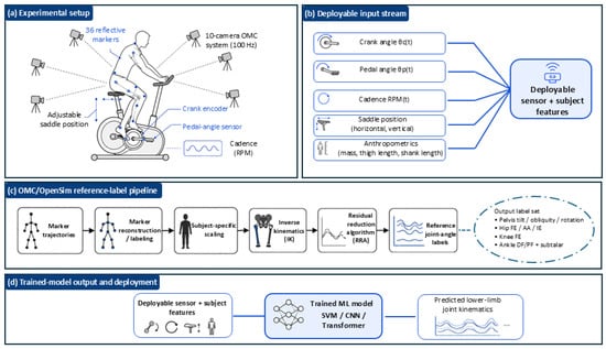
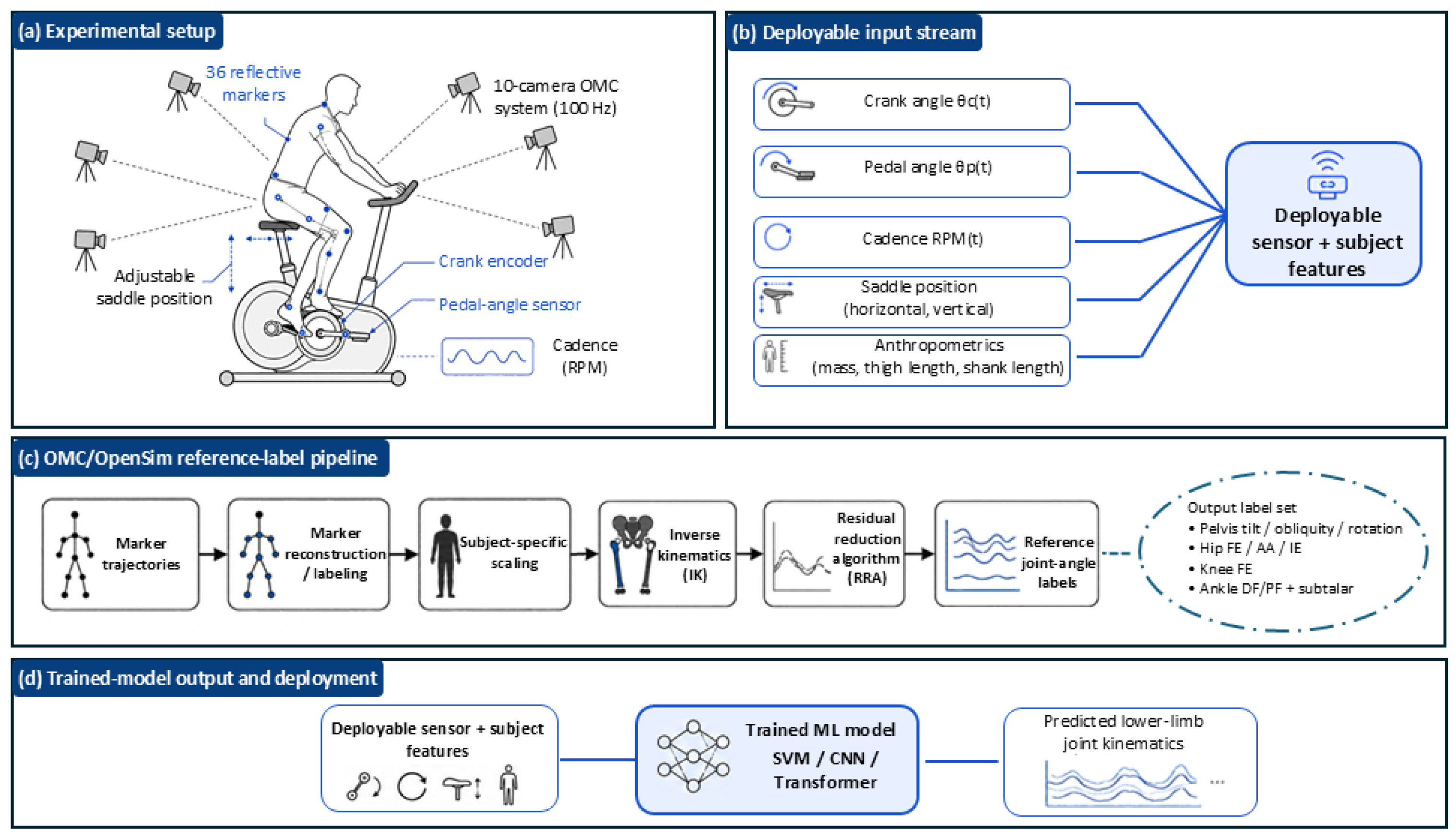
The overall experimental, reference-kinematic, and model-deployment workflows are summarized in Figure 1. The figure distinguishes the laboratory optical motion capture and OpenSim (Version 4.4, Stanford University, Stanford, CA, USA) pipeline used to generate reference joint-angle labels from the deployable sensor and participant-specific features used by the trained ML models.

Figure 1. Overview of the experimental, reference-kinematic, and model-deployment workflows. (a) Experimental setup showing the adjustable saddle position, 36 reflective markers, 10-camera optical motion capture system, crank encoder, pedal-angle sensor, and cadence measurement. (b) Deployable input stream comprising crank angle, pedal angle, cadence, horizontal and vertical saddle positions, and participant anthropometric characteristics. (c) Optical motion capture and OpenSim reference-label pipeline, including marker-trajectory reconstruction, subject-specific model scaling, inverse kinematics, and the Residual Reduction Algorithm, used to obtain the reference pelvis and lower-limb joint-angle labels. (d) Deployment workflow in which the deployable sensor and participant features are provided to the trained SVM, CNN, or Transformer model to predict lower-limb joint kinematics.

2.1. Data Collection

Fifteen healthy individuals (10 males, 5 females; age = 28.3 ± 3.4 years; height = 174 ± 7 cm; body mass = 71.2 ± 11.6 kg) were recruited for this study. Ethics approval was obtained from the University of Calgary Conjoint Health Research Ethics Board (REB #23-1803; approved 16 July 2024), and written informed consent was obtained from all participants prior to testing. All participants were right-leg dominant and reported no musculoskeletal disorders within three months prior to the test date.

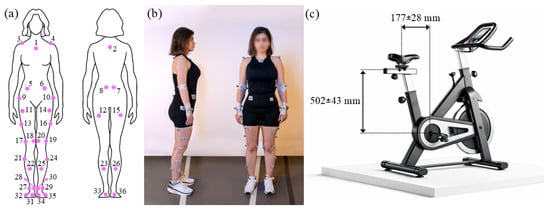
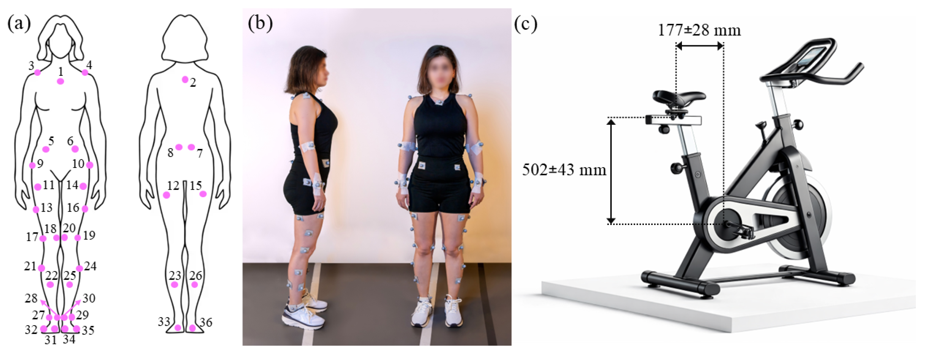
Experiments were performed on a stationary cycling ergometer trainer (Echelon Connect EX-5, Echelon Fitness Multimedia LLC, Chattanooga, TN, USA) equipped with a 17 cm crank arm. Participants’ lower-body motion was recorded by tracking the trajectories of reflective markers using a 10-camera Vicon motion capture system (Vicon Motion Systems Ltd., Oxford, UK) at a sampling rate of 100 Hz. Thirty-six passive reflective skin markers, each 18 mm in diameter, were placed on anatomical landmarks as shown in Figure 2a,b. The optical motion capture (OMC) system was synchronized with the sensor system integrated into the stationary bike, including tri-axial pedal force sensors (Sensix, Poitiers, France) and a crank encoder (RLS-MR076G060A120N00, RLS Merilna tehnika d.o.o., Komenda, Slovenia), sampling at 250 Hz. The saddle position was adjusted at two vertical and two horizontal levels based on each participant’s height. The horizontal and vertical distances from the saddle to the bottom bracket ranged from 149 to 205 mm and 459 to 545 mm, respectively (Figure 2c). Each participant performed 60 pedaling cycles, repeated 8 times, using different permutations of cadence and saddle position: one trial at their fastest sustainable pace (fast), one at a self-selected pace (normal), and two trials each at different vertical and horizontal saddle positions. To minimize fatigue effects, a 5 min rest period was provided between trials.

Figure 2. (a,b) Thirty-six reflective markers were placed on the skin at the following anatomical landmarks: 2nd and 5th metatarsal heads (31, 32, 34, 35), calcanei (33, 36), medial and lateral malleoli (27, 28, 29, 30), shanks (21–26), medial and lateral femoral epicondyles (17–20), thighs (11–16), greater trochanters (9, 10), anterior and posterior superior iliac spines (5–8), acromia (3, 4), C7 vertebra (2), and the sternoclavicular joint (1). (c) Saddle horizontal and vertical positions were adjusted based on participant height, with adjustment ranges of 56 mm and 86 mm in the horizontal and vertical directions, respectively. Distances were measured from the bottom bracket.

2.2. Data Post-Processing

Marker trajectories were reconstructed in Vicon Nexus (Version 2.15, Vicon Motion Systems Ltd., Oxford, UK). A subject-specific musculoskeletal model was generated for each subject by scaling the musculoskeletal model of Lai et al. [55] using anatomical marker data and the OpenSim Scale Tool [25]. In addition, functional knee joint centers were estimated from the cycling trials using the Symmetrical Center of Rotation Estimation (SCoRE) method [56], and hip joint centers were estimated using the Harrington method [57]. These subject-specific joint center estimates were used together with anatomical markers to improve scaling of the model to each participant’s anthropometry.

The musculoskeletal model included 33 degrees of freedom, covering the pelvis in the ground frame (anterior–posterior tilt, adduction–abduction, internal–external rotation, anterior–posterior translation, vertical translation, and medial–lateral translation), hips (flexion–extension, abduction–adduction, and internal–external rotation), knees (flexion–extension), ankles (dorsi/plantar flexion, and subtalar supination–pronation), metatarsophalangeal joints (dorsi/plantar flexion), lumbar region (flexion–extension, right–left bending, and right–left rotation), shoulders (flexion–extension, abduction–adduction, and internal–external rotation), and elbows (flexion–extension, and supination–pronation). Because lower-limb joint kinematics were the focus of the present cycling application, subsequent analyses were restricted to pelvis, hip, knee, ankle, and subtalar joint motions. Joint angles were first computed using the OpenSim Inverse Kinematics (IK) tool based on the scaled models and reconstructed marker trajectories.

Following IK, the Residual Reduction Algorithm (RRA) was applied to improve dynamic consistency between the prescribed kinematics and the measured external forces. To represent pelvis–saddle interaction, actuators were applied to all six degrees of freedom of the pelvis with sufficient capacity to support up to one body weight. In addition, torque actuators were assigned to the rotational degrees of freedom to ensure that the prescribed motions could be reproduced. Reserve actuator usage was evaluated according to the recommendations of Hicks et al. [58] by expressing the reserve torque as a percentage of the corresponding peak post-RRA net joint moment. All analyzed lower-limb degrees of freedom satisfied the recommended criterion of reserve actuator contributions remaining below 5% across all trials. The maximum observed reserve contribution was 4.2% (left hip internal/external rotation), whereas all remaining degrees of freedom were below 2.0%. In this framework, residual actuators accounted for unmeasured pelvis–saddle interactions, whereas reserve actuators supplied supplementary torque to lower-body degrees of freedom to facilitate convergence and improve dynamic consistency.

OpenSim RRA-adjusted kinematics were used as the laboratory reference for model training and evaluation rather than as error-free ground truth. These reference kinematics are affected by marker placement, soft-tissue artifact, model scaling, joint-center estimation, inverse kinematics, and RRA processing. Previous lower-limb kinematic validation studies have reported that model-based or motion-capture-derived joint-angle errors are generally smaller for sagittal-plane movements and larger for frontal- and transverse-plane movements [59]. Therefore, the reported ML prediction errors in the present study represent differences relative to the OpenSim RRA-adjusted reference kinematics and may include both model-prediction error and uncertainty in the reference kinematic pipeline. This limitation is especially important when interpreting non-sagittal joint angles, where smaller movement amplitudes and greater plane-specific uncertainty can increase apparent prediction error.

2.3. Development of ML Models

2.3.1. Feature Selection and Input Preparation

Before machine learning analysis, the recorded data were segmented into individual pedaling cycles. The most relevant features of the target variables were identified through an iterative selection process that evaluated cross-validation prediction performance for each candidate feature combination. While a formal systematic importance analysis (e.g., permutation importance, SHAP values, recursive feature elimination, or mutual information) was not applied, the selected feature set was empirically validated through model performance. The final feature set included the vertical and horizontal distances from the bottom bracket to the saddle, crank and pedal angles, cycling cadence, as well as the participants’ body mass and the measured lengths of their shank and thigh. These features were organized into sequences of consecutive, overlapping windows. Each window was shifted by one sample across the dataset to generate consecutive overlapping input sequences for each target value. The window length was selected based on the temporal characteristics of the cycling task and the sampling frequency of the deployable sensor stream, following the general approach used in previous ML-based biomechanical prediction studies in which window duration is selected relative to the movement cycle [26,60]. In the present study, the cadence range of 50–80 rpm corresponded to an approximate crank-cycle duration of 0.75–1.20 s. Consequently, a 0.2 s window represented approximately 17–27% of one crank revolution. This duration provided sufficient temporal context to capture local within-cycle variations in crank angle, pedal angle, and cadence-dependent input patterns while maintaining low prediction latency for potential real-time implementation. Because the crank encoder and pedal sensors were sampled at 250 Hz, each window contained 50 consecutive samples. Cadence was also included as an input feature to account for differences in cycle timing among participants and experimental conditions.

The ML models predicted joint kinematic parameters, including hip flexion/extension, hip adduction/abduction, hip internal/external rotation, knee flexion/extension, ankle dorsi/plantar flexion, subtalar pronation/supination, pelvis anterior/posterior tilt, pelvis internal/external rotation, and pelvis adduction/abduction. The models were implemented as multi-output regressors, predicting all target variables simultaneously.

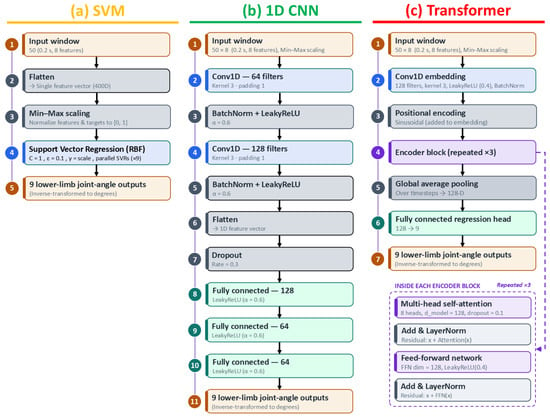
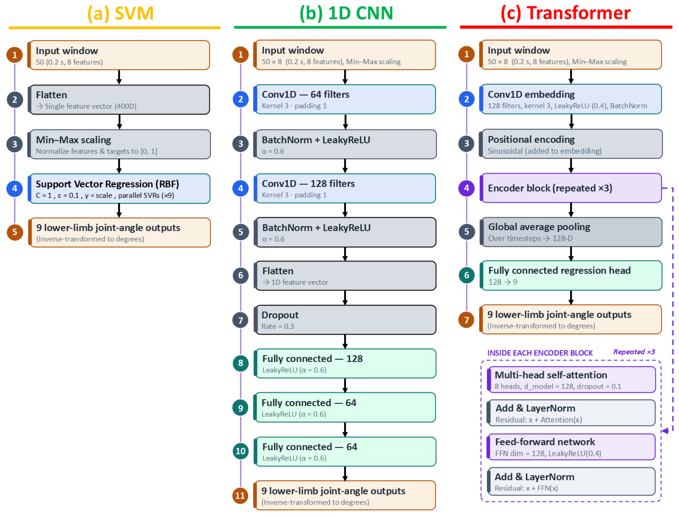
Given the sensitivity of machine learning models to feature scale, consistent feature scaling was applied across all models to improve convergence and overall performance. The MinMaxScaler function from the scikit-learn library (Version 1.8) was used to normalize both input features and target variables to a range of (0, 1). After predictions were made, target values were rescaled to their original range using the same scaler, ensuring interpretability of the results. This consistent preprocessing step enabled effective model training and fair comparisons between models. The model-specific architectures are illustrated in Figure 3, and the final implementation details and hyperparameter configurations used for model development are summarized in Table 1.

Figure 3. Architectures of the regression models used to predict lower-limb joint kinematics. All models received overlapping 0.2 s input windows comprising 50 samples and eight input features and produced nine lower-limb joint-angle outputs. (a) Support Vector Machine (SVM) regression, in which each input window was flattened, normalized, and provided to nine parallel ε-support vector regression (SVR) models using a radial basis function (RBF) kernel. (b) One-dimensional convolutional neural network (CNN) comprising two convolutional layers, batch normalization, LeakyReLU activation, dropout, and three fully connected hidden layers. (c) Encoder-only Transformer architecture comprising a Conv1D input embedding, fixed sinusoidal positional encoding, three multi-head self-attention encoder blocks, global average pooling, and a fully connected nine-output regression head.

Table 1. Final architecture, optimization, regularization, and training hyperparameters used for the SVM, CNN, and Transformer models.

Configuration	SVM	CNN	Transformer
Input-window duration	0.2 s	0.2 s	0.2 s
Input samples per window	50	50	50
Input features	8	8	8
Input representation	Flattened 400-dimensional feature vector	50 × 8 sequence	50 × 8 sequence
Output variables	9	9	9
Multi-output strategy	Nine parallel ε-SVR regressors (one per output)	Single nine-unit output layer	Single nine-unit output layer
Model architecture	RBF Support Vector Regression	Two-layer 1D CNN	Encoder-only Transformer (3 encoder blocks)
Kernel/embedding	RBF kernel	Conv1D	Conv1D embedding
C	1	N/A	N/A
Epsilon (ε)	0.1	N/A	N/A
Kernel size	N/A	3	3
Padding	N/A	1	1
Convolutional filters/embedding dimension	N/A	64, 128	128
Activation function	N/A	LeakyReLU (α = 0.6)	LeakyReLU (α = 0.4)
Fully connected layers	N/A	128, 64, 64	128 → 9 regression head
Attention heads	N/A	N/A	8
Feed-forward dimension	N/A	N/A	128
Positional encoding	N/A	N/A	Fixed sinusoidal
Dropout	N/A	0.3	0.1
Training algorithm/optimizer	LIBSVM ε-SVR solver	AdamW	AdamW
Loss/objective function	ε-insensitive SVR objective	Mean squared error	Mean squared error
Initial learning rate	N/A	1 × 10−4	1 × 10−5
Batch size	N/A	64	64
Learning-rate scheduler	N/A	StepLR (step = 5, γ = 0.1)	StepLR (step = 5, γ = 0.1)
Maximum epochs	N/A	100	100
Early-stopping patience	N/A	10 epochs	10 epochs

Abbreviations: RBF, radial basis function; SVR, support vector regression; CNN, convolutional neural network. All models received overlapping 0.2 s input windows comprising eight input features (crank angle, pedal angle, cadence, horizontal and vertical saddle positions, body mass, thigh length, and shank length) and predicted nine lower-limb joint angles.

2.3.2. Support Vector Machine (SVM)

The core mechanism of SVM regression employs a kernel function to project input feature vectors into a higher-dimensional space, identifying a hyperplane that fits the data within a user-defined error margin (epsilon-tube). This formulation makes SVM particularly effective for small-to-medium-sized datasets and less sensitive to outliers within the epsilon margin. In this study, after extensive hyperparameter tuning, the optimal settings were determined as follows: ε = 0.1 (selected from 0.001, 0.01, 0.1, and 1), cost parameter C = 1 (chosen from 0.1, 1, 10, and 100), and the radial basis function (RBF) as the kernel function (selected from “linear”, “RBF”, and “sigmoid”). These settings yielded the best performance in capturing the non-linear relationships within the data.

2.3.3. Convolutional Neural Network (CNN)

The CNNs automatically extract hierarchical spatial features from local temporal windows using convolutional filters, enabling efficient pattern recognition without requiring manual feature engineering. As a specialized type of neural network (NN) model, CNNs have demonstrated remarkable performance in time-series forecasting [26]. The architecture included two 1D convolutional layers with 64 and 128 filters, respectively, a kernel size of 3, and padding of 1 to maintain sequence length. Each convolutional layer was followed by a batch normalization layer to improve training stability, and a “LeakyReLU (alpha = 0.6)” activation function was used. The output of the final convolutional layer was flattened and passed through three fully connected layers with 128, 64, and 64 units, respectively, each using “LeakyReLU (alpha = 0.6)” activation. A dropout layer with a rate of 0.3 was applied before the fully connected layers to mitigate overfitting. The final output layer had nine units to predict the target joint angles. The model was trained using the “AdamW” optimizer with a learning rate of 0.0001 and “mean squared error” as the loss function. A StepLR learning rate scheduler was used, reducing the learning rate by a factor of 0.1 every five epochs. Training was conducted with a batch size of 64 for a maximum of 100 epochs. Additionally, the “EarlyStopping” function was employed to monitor the validation loss and stop training if there was no improvement after ten epochs. The best-performing model on the validation set was saved during training. To evaluate performance, predictions on the test set were inverse-transformed to the original scale and compared to the reference values using root mean square error (RMSE). In the CNN model, a grid search was conducted to determine the optimal activation function (among “LeakyReLU”, “ReLU”, “Sigmoid”, “GELU”, and “Tanh”), optimizer (among “Adam”, “AdamW”, “RMSProp”, and “SGD”), learning rate (among 0.01, 0.001, and 0.0001), and number of neurons (among 64, 128, 256, and 512).

2.3.4. Transformer

Transformers are a specialized type of neural network model that has demonstrated remarkable performance in various tasks, including time-series prediction [43,44,45]. In this study, a multi-output Transformer model with multiple encoder blocks was employed to estimate joint kinematics. The model architecture began with an input layer, followed by a Conv1D layer with 128 filters, a kernel size of 3, and a “LeakyReLU” activation function, together with batch normalization and fixed sinusoidal positional encoding. Positional encoding was incorporated to inject temporal sequence-order information into the input embeddings, enabling the model to differentiate between positions within each input window. The core of the model consisted of three Transformer encoder blocks, each comprising multi-head self-attention (8 heads) and a feed-forward dimension of 128. No decoder was used because the model employed an encoder-only architecture for direct multi-output regression. Dropout (0.1) was applied for regularization, and the final layer comprised a fully connected nine-unit regression output layer. The “AdamW” optimizer, with a learning rate of 1 × 10⁻⁵, was utilized for weight optimization, alongside “mean squared error” as the loss function. A StepLR learning rate scheduler was used, reducing the learning rate by a factor of 0.1 every five epochs. The “EarlyStopping” function monitored the validation loss and stopped training if there was no improvement after ten epochs. The batch size was set to 64, and the model was trained for a maximum of 100 epochs. Optimal parameters, including activation functions, optimizer, learning rate, and neuron count, were determined through grid search.

2.4. Performance Evaluation

Training an ML model to predict biomechanical targets generally serves two primary applications: (1) intra-subject models, where the model is trained using data from a specific individual and then used to predict biomechanical parameters for unseen cycles from the same individual; and (2) inter-subject models, where the model is trained using data from a broader population and applied to new, unseen individuals.

For the intra-subject evaluation, data were partitioned separately for each participant at the pedaling-cycle level. Specifically, 70% of each participant’s pedaling cycles were randomly assigned to the model-development set, while the remaining 30% were reserved as the independent test set. The model-development set was subsequently divided into training and validation subsets, with 80% of the cycles used for training and the remaining 20% for validation. Consequently, the effective intra-subject partition consisted of 56% training, 14% validation, and 30% testing. The validation subset was used for early stopping and model selection, whereas the independent test set was reserved exclusively for final performance evaluation. All samples belonging to a given pedaling cycle were assigned to a single partition to prevent frame-level data leakage.

For the inter-subject evaluation, a leave-one-subject-out cross-validation strategy was adopted to assess model generalizability to unseen participants. In each fold, all data from one participant were reserved as the independent test set, whereas data from the remaining 14 participants were used for model development. Within the model-development dataset, 80% of the pedaling cycles were used for training and the remaining 20% for validation. The validation subset was used for early stopping and model selection. No data from the held-out participant were used during training, validation, model selection, or hyperparameter tuning, thereby preventing subject-level data leakage.

RMSE between the OpenSim RRA-adjusted reference kinematics and predicted targets was calculated for both intra-subject and inter-subject evaluations. The reference kinematics were defined as the adjusted joint angles obtained from OpenSim RRA following IK. RMSE was computed for each cycle and participant to enable direct comparison among the ML models. To account for differences in signal magnitude across targets, normalized RMSE (nRMSE) was calculated as the RMSE divided by the range of the corresponding OpenSim RRA-adjusted reference joint angle and expressed as a percentage. The reported RMSE and nRMSE values represent the average cross-validation results across all participants. For descriptive comparison of joint-angle amplitude, the minimum and maximum values of each reference and predicted joint-angle waveform were identified over one crank revolution, and range of motion (ROM) was calculated as the maximum value minus the minimum value.

2.5. Statistical Analysis

Statistical analyses were conducted to compare nRMSE among the three machine learning models (Transformer, CNN, and SVM) for each joint movement in the intra-subject and inter-subject evaluations. Because all three model outputs were available for the same participants, analyses were performed using a repeated-measures framework. Normality was assessed using the Shapiro–Wilk test on paired difference scores between models. When normality assumptions were satisfied, a one-way repeated-measures analysis of variance (ANOVA) was used to examine differences among the three models. When normality assumptions were violated, the non-parametric Friedman test was applied. When a significant omnibus effect was detected, post hoc pairwise comparisons were performed between Transformer vs. CNN, Transformer vs. SVM, and CNN vs. SVM using paired-samples t-tests or Wilcoxon signed-rank tests, as appropriate. Holm adjustment was applied to account for multiple pairwise comparisons. Effect sizes were reported as partial eta squared (η_p²) for repeated-measures ANOVA, Kendall’s W for Friedman tests, Cohen’s dz for paired t-tests, and rank-biserial correlation (r) for Wilcoxon signed-rank tests. All analyses were performed using Python (Version 3.13.1, Python Software Foundation, Wilmington, DE, USA), and statistical significance was set at α = 0.05.

3. Results

Model performance was evaluated through intra-subject and inter-subject examinations using OpenSim RRA-adjusted reference joint angles obtained following inverse kinematics. The reported inference times correspond to the total time required to process a 60 s recording on the evaluation workstation (NVIDIA GeForce RTX 5080 GPU, NVIDIA Corporation, Santa Clara, CA, USA) and exclude model training. The CNN required approximately 0.5 s, followed by the Transformer (approximately 4 s) and the SVM (approximately 7 s).

3.1. Intra-Subject Comparison

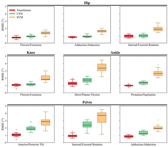
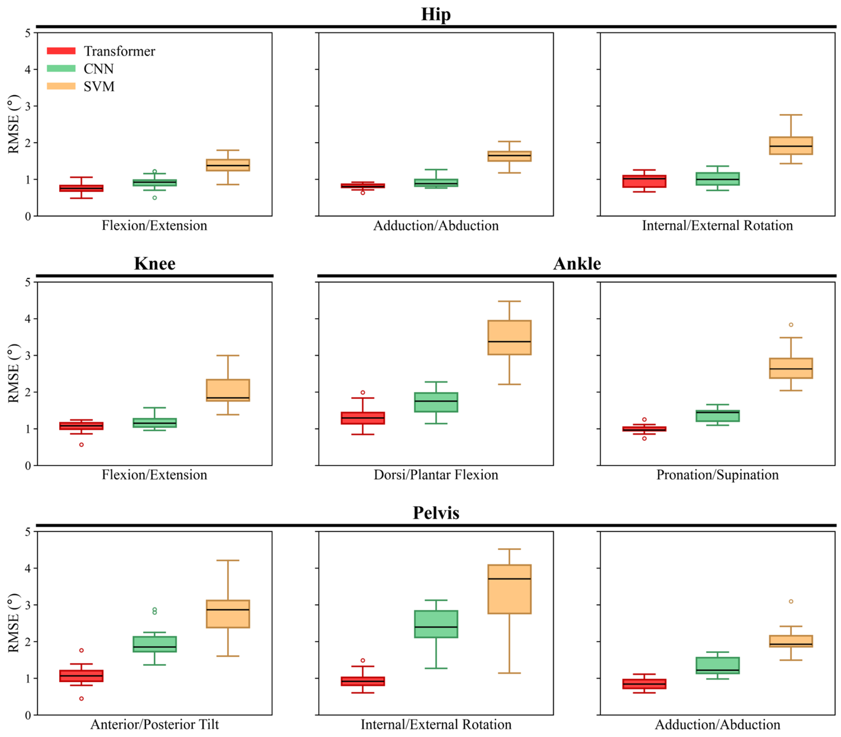
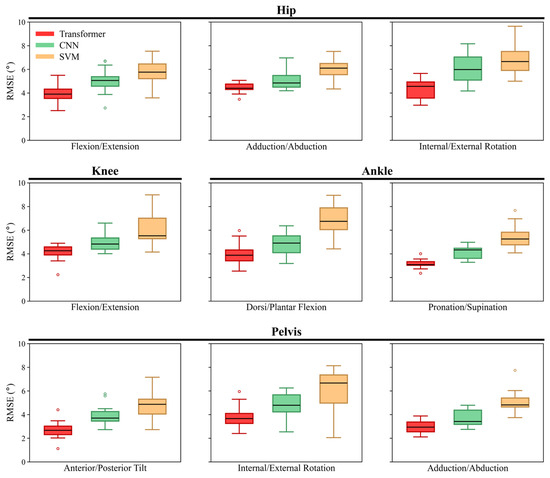
Table 2 summarizes the mean ± SD nRMSE values together with omnibus repeated-measures test results, post hoc pairwise comparisons, and effect sizes for the intra-subject evaluation. Overall, the three models differed significantly for all joint movements, with large effect sizes, and the Transformer consistently showed the lowest or comparable nRMSE values, whereas the SVM generally exhibited the highest errors. Figure 4 shows the corresponding RMSE distributions across participants for each joint movement. The Transformer’s RMSE ranged from 0.8° ± 0.2° (hip flexion/extension) to 1.3° ± 0.3° (ankle dorsi/plantar flexion), with the minimum error among all participants observed in pelvis anterior/posterior tilt (0.4°) and the highest in ankle dorsi/plantar flexion (2.0°). The CNN’s RMSE ranged from 0.9° ± 0.2° (hip flexion/extension) to 2.4° ± 0.6° (pelvis internal/external rotation), with the minimum error across participants at 0.5° in hip flexion/extension and the maximum at 3.1° in pelvis internal/external rotation. The SVM exhibited the highest error rates among the three models, with RMSE values ranging from 1.4° ± 0.3° (hip flexion/extension) to 3.4° ± 0.7° (ankle dorsi/plantar flexion). The lowest overall error across participants was 0.8° in hip flexion/extension, while the highest was 4.5° in pelvis internal/external rotation. Overall, the Transformer model achieved the best performance in 7 out of 9 joint angle predictions, reinforcing its superior accuracy in modeling joint kinematics. Among all joint angles examined, hip flexion/extension consistently demonstrated lower RMSE and nRMSE values across all three models (Transformer, CNN, and SVM), indicating relatively higher prediction accuracy for this joint compared to others.

Table 2. Mean ± SD nRMSE for intra-subject evaluation, together with omnibus repeated-measures test results, effect sizes, and Holm-adjusted post hoc pairwise comparisons among the Transformer, CNN, and SVM models for each joint movement.

Intra-Subject Examination	nRMSE			Omnibus Test		Post Hoc
	T †	C †	S †	p-Value	Effect Size (ηp2/W) ‡	Pairwise Comparison	p-Value	Effect Size (dz/r) ‡ ‡
Hip Flexion/Extension	0.01 ± 0.01	0.01 ± 0.01	0.02 ± 0.01	<0.01 *	W = 0.88	T vs. C	<0.01 *	r = −0.66
						T vs. S	<0.01 *	r = −0.88
						C vs. S	<0.01 *	r = −0.88
Hip Adduction/Abduction	0.10 ± 0.01	0.12 ± 0.02	0.21 ± 0.04	<0.01 *	W = 0.84	T vs. C	<0.01 *	r = −0.75
						T vs. S	<0.01 *	r = −0.88
						C vs. S	<0.01 *	r = −0.88
Hip Internal/External Rotation	0.10 ± 0.02	0.10 ± 0.02	0.20 ± 0.04	<0.01 *	W = 0.76	T vs. C	0.89	r = −0.05
						T vs. S	<0.01 *	r = −0.88
						C vs. S	<0.01 *	r = −0.88
Knee Flexion/Extension	0.01 ± 0.01	0.01 ± 0.01	0.02 ± 0.01	<0.01 *	W = 0.80	T vs. C	0.04 *	r = −0.54
						T vs. S	<0.01 *	r = −0.88
						C vs. S	<0.01 *	r = −0.88
Ankle Dorsi/Plantar Flexion	0.03 ± 0.01	0.04 ± 0.01	0.08 ± 0.02	<0.01 *	ηp2 = 0.91	T vs. C	<0.01 *	dz = −1.94
						T vs. S	<0.01 *	dz = −3.54
						C vs. S	<0.01 *	dz = −2.84
Subtalar Pronation/Supination	0.08 ± 0.01	0.12 ± 0.02	0.23 ± 0.04	<0.01 *	ηp2 = 0.93	T vs. C	<0.01 *	dz = −1.75
						T vs. S	<0.01 *	dz = −3.62
						C vs. S	<0.01 *	dz = −3.47
Pelvis Anterior/Posterior Tilt	0.12 ± 0.03	0.22 ± 0.05	0.32 ± 0.07	<0.01 *	ηp2 = 0.86	T vs. C	<0.01 *	dz = −1.94
						T vs. S	<0.01 *	dz = −2.59
						C vs. S	<0.01 *	dz = −2.64
Pelvis Internal/External Rotation	0.14 ± 0.04	0.35 ± 0.09	0.49 ± 0.13	<0.01 *	ηp2 = 0.84	T vs. C	<0.01 *	dz = −2.94
						T vs. S	<0.01 *	dz = −2.64
						C vs. S	<0.01 *	dz = −1.15
Pelvis Adduction/Abduction	0.09 ± 0.02	0.14 ± 0.03	0.21 ± 0.04	<0.01 *	ηp2 = 0.88	T vs. C	<0.01 *	dz = −1.71
						T vs. S	<0.01 *	dz = −3.12
						C vs. S	<0.01 *	dz = −2.22

*: Indicates statistical significance at p < 0.05. ^† T: Transformer; C: CNN; S: SVM. ^‡ Partial eta squared (η_p²) for parametric (ANOVA) and Kendall’s W for non-parametric (Friedman) tests. ^{‡ ‡} Cohen’s dz for parametric and rank-biserial r for non-parametric post hoc comparisons.

Figure 4. Boxplots of RMSE across participants for each joint movement in the intra-subject evaluation, grouped by anatomical region (hip, knee and ankle, and pelvis), for the Transformer, CNN, and SVM models. Boxes represent the interquartile range, center lines denote the median, whiskers extend to 1.5 times the interquartile range, and circles indicate outliers.

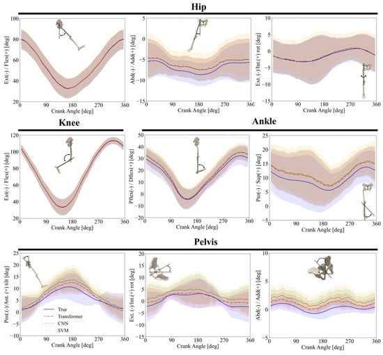
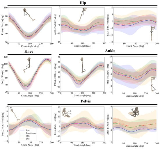
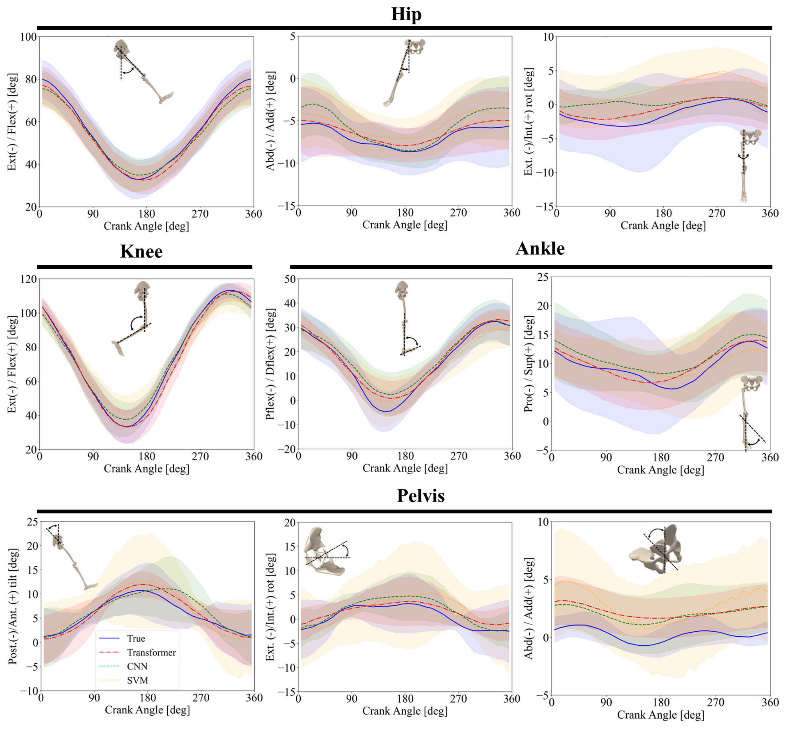
Figure 5 depicts the intra-subject joint angle predictions over multiple cycles, with each subplot representing a different joint movement. It compares the OpenSim RRA-adjusted reference motion (solid blue), with predictions from the Transformer model (red dash-dot), CNN (green dashed), and SVM (orange dotted). The Transformer model consistently outperformed the other models, particularly in rotational movements. While all three models captured the general trends well, the SVM exhibited greater errors. Complex movements such as pelvis anterior/posterior tilt, pelvis adduction/abduction, and pelvis internal/external rotation clearly highlighted the Transformer’s advantage. Both the CNN and SVM models produced greater errors than the Transformer in predicting these joint angles.

Figure 5. Intra-subject comparison of joint angles predicted by the ML models and those obtained from OpenSim RRA-adjusted kinematics across one crank revolution (mean ± SD). The OpenSim RRA-adjusted reference kinematics are shown as a solid blue line, while the Transformer, CNN, and SVM predictions are distinguished using different line styles (dash-dot, dashed, and dotted, respectively) together with different colors to improve visual discrimination.

Table 3 presents the minimum and maximum joint angles and corresponding ROM values for the OpenSim RRA-adjusted reference kinematics and the predictions from each model in the intra-subject evaluation. The predicted ROMs generally agreed closely with the reference values for hip and knee flexion/extension, whereas greater differences were observed for pelvis anterior/posterior tilt and pelvis internal/external rotation.

Table 3. Minimum and maximum joint angles and corresponding range of motion (ROM) for the OpenSim RRA-adjusted reference kinematics and model predictions in the intra-subject evaluation. All values are reported in degrees.

Joint Movement	Reference Min to Max (ROM)	Transformer Min to Max (ROM)	CNN Min to Max (ROM)	SVM Min to Max (ROM)
Hip flexion/extension	32.1 to 80.3 (48.2)	31.1 to 78.9 (47.8)	31.5 to 79.1 (47.6)	33.4 to 81.6 (48.2)
Hip adduction/abduction	−8.8 to −5.1 (3.7)	−7.4 to −4.6 (2.8)	−7.6 to −4.8 (2.8)	−6.2 to −3.5 (2.7)
Hip internal/external rotation	−3.3 to 0.9 (4.2)	−3.2 to 1.1 (4.3)	−3.2 to 1.1 (4.3)	−2.4 to 2.3 (4.7)
Knee flexion/extension	34.7 to 114.8 (80.1)	34.5 to 114.9 (80.4)	34.4 to 114.8 (80.4)	35.3 to 115.4 (80.1)
Ankle dorsi/plantar flexion	−4.4 to 32.6 (37.0)	−3.5 to 35.1 (38.6)	−2.9 to 35.7 (38.6)	−1.1 to 38.0 (39.1)
Subtalar pronation/supination	5.4 to 13.9 (8.5)	7.1 to 15.8 (8.7)	7.4 to 16.1 (8.7)	8.5 to 17.4 (8.9)
Pelvis anterior/posterior tilt	1.7 to 10.9 (9.2)	1.1 to 13.1 (12.0)	2.1 to 14.0 (11.9)	3.4 to 14.9 (11.5)
Pelvis internal/external rotation	−2.2 to 3.7 (5.9)	−0.5 to 3.9 (4.4)	0.4 to 5.1 (4.7)	1.2 to 5.8 (4.6)
Pelvis adduction/abduction	−0.8 to 1.2 (2.0)	0.2 to 1.9 (1.7)	0.7 to 2.6 (1.9)	1.0 to 3.2 (2.2)

3.2. Inter-Subject Comparison

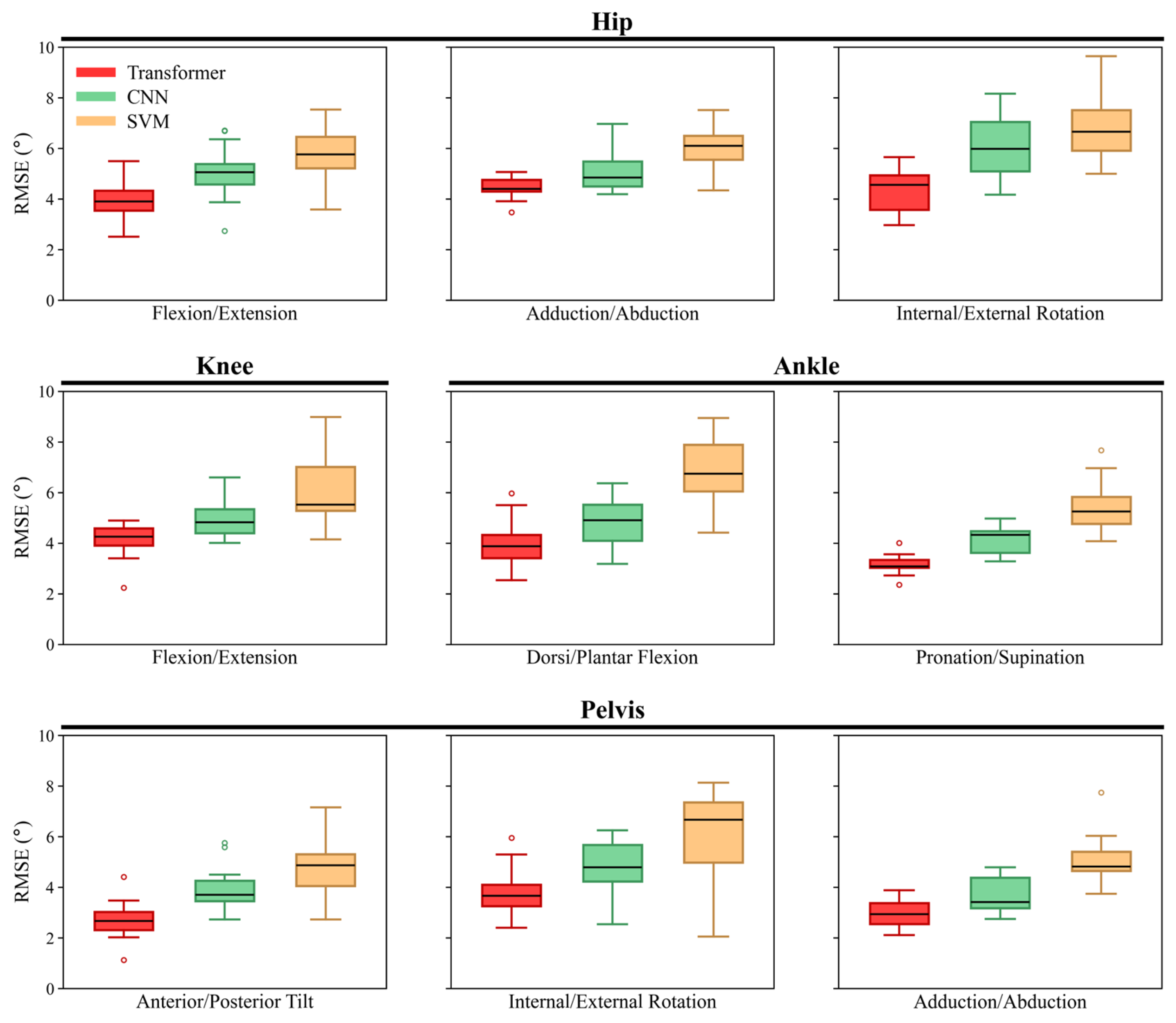
Table 4 summarizes the mean ± SD nRMSE values together with omnibus repeated-measures test results, post hoc pairwise comparisons, and effect sizes for the inter-subject evaluation. Similar to intra-subject test, the Transformer model consistently produced the lowest nRMSE values for most joint movements, the CNN generally showed intermediate performance, and the SVM yielded the largest errors overall. Figure 6 shows the corresponding RMSE distributions across participants for each joint movement. The RMSE of the Transformer model ranged from 2.7° ± 0.7° (pelvis anterior/posterior tilt) to 4.4° ± 0.4° (hip adduction/abduction), with the minimum error across all participants observed in pelvis anterior/posterior tilt (1.1°), and the highest in ankle dorsi/plantar flexion prediction (6.0°) (Figure 6). The CNN’s RMSE ranged from 3.7° ± 0.7° (pelvis adduction/abduction) to 6.1° ± 1.3° (hip internal/external rotation), with the minimum error of 2.5° in pelvis internal/external rotation and the highest of 8.2° in hip internal/external rotation across all participants (Figure 6). The SVM exhibited the greatest errors, with RMSE values ranging from 4.8° ± 1.2° (pelvis anterior/posterior tilt) to 7.0° ± 1.4° (hip internal/external rotation) (Figure 6). The minimum error was 2.1° in pelvis internal/external rotation, and the maximum was 9.7° in hip internal/external rotation. Based on nRMSE values, hip flexion/extension and knee flexion/extension showed the smallest relative prediction errors across models, whereas pelvis internal/external rotation and hip internal/external rotation showed comparatively larger relative errors and greater variability, consistent with the intra-subject evaluation.

Table 4. Mean ± SD nRMSE for inter-subject evaluation, together with omnibus repeated-measures test results, effect sizes, and Holm-adjusted post hoc pairwise comparisons among the Transformer, CNN, and SVM models for each joint movement.

Inter-Subject Examination	nRMSE			Omnibus Test		Post Hoc
	T †	C †	S †	p-Value	Effect Size (ηp2/W) ‡	Pairwise Comparison	p-Value	Effect Size (dz/r) ‡ ‡
Hip Flexion/Extension	0.06 ± 0.01	0.07 ± 0.02	0.08 ± 0.02	<0.01 *	W = 0.76	T vs. C	<0.01 *	r = −0.73
						T vs. S	<0.01 *	r = −0.87
						C vs. S	<0.01 *	r = −0.88
Hip Adduction/Abduction	0.56 ± 0.08	0.64 ± 0.13	0.77 ± 0.13	<0.01 *	W = 0.84	T vs. C	<0.01 *	r = −0.75
						T vs. S	<0.01 *	r = −0.88
						C vs. S	<0.01 *	r = −0.88
Hip Internal/External Rotation	0.45 ± 0.08	0.62 ± 0.12	0.71 ± 0.14	<0.01 *	W = 0.94	T vs. C	<0.01 *	r = −0.88
						T vs. S	<0.01 *	r = −0.88
						C vs. S	<0.01 *	r = −0.82
Knee Flexion/Extension	0.05 ± 0.01	0.06 ± 0.01	0.07 ± 0.01	<0.01 *	W = 0.70	T vs. C	<0.01 *	r = −0.85
						T vs. S	<0.01 *	r = −0.87
						C vs. S	<0.01 *	r = −0.79
Ankle Dorsi/Plantar Flexion	0.09 ± 0.02	0.11 ± 0.02	0.16 ± 0.03	<0.01 *	ηp2 = 0.80	T vs. C	<0.01 *	dz = −1.46
						T vs. S	<0.01 *	dz = −2.31
						C vs. S	<0.01 *	dz = −1.58
Subtalar Pronation/Supination	0.26 ± 0.03	0.35 ± 0.04	0.45 ± 0.08	<0.01 *	ηp2 = 0.81	T vs. C	<0.01 *	dz = −1.43
						T vs. S	<0.01 *	dz = −2.34
						C vs. S	<0.01 *	dz = −1.80
Pelvis Anterior/Posterior Tilt	0.30 ± 0.08	0.44 ± 0.09	0.55 ± 0.12	<0.01 *	ηp2 = 0.72	T vs. C	<0.01 *	dz = −1.25
						T vs. S	<0.01 *	dz = −1.70
						C vs. S	<0.01 *	dz = −1.77
Pelvis Internal/External Rotation	0.55 ± 0.14	0.70 ± 0.17	0.88 ± 0.24	<0.01 *	ηp2 = 0.56	T vs. C	<0.01 *	dz = −0.99
						T vs. S	<0.01 *	dz = −1.27
						C vs. S	<0.01 *	dz = −0.83
Pelvis Adduction/Abduction	0.31 ± 0.06	0.38 ± 0.07	0.52 ± 0.10	<0.01 *	W = 0.88	T vs. C	<0.01 *	r = −0.78
						T vs. S	<0.01 *	r = −0.88
						C vs. S	<0.01 *	r = −0.88

*: Indicates statistical significance at p < 0.05. ^† T: Transformer; C: CNN; S: SVM. ^‡ Partial eta squared (η_p²) for parametric (ANOVA) and Kendall’s W for non-parametric (Friedman) tests. ^{‡ ‡} Cohen’s dz for parametric and rank-biserial r for non-parametric post hoc comparisons.

Figure 6. Boxplots of RMSE across participants for each joint movement in the inter-subject evaluation, grouped by anatomical region (hip, knee and ankle, and pelvis), for the Transformer, CNN, and SVM models. Boxes represent the interquartile range, center lines denote the median, whiskers extend to 1.5 times the interquartile range, and circles indicate outliers.

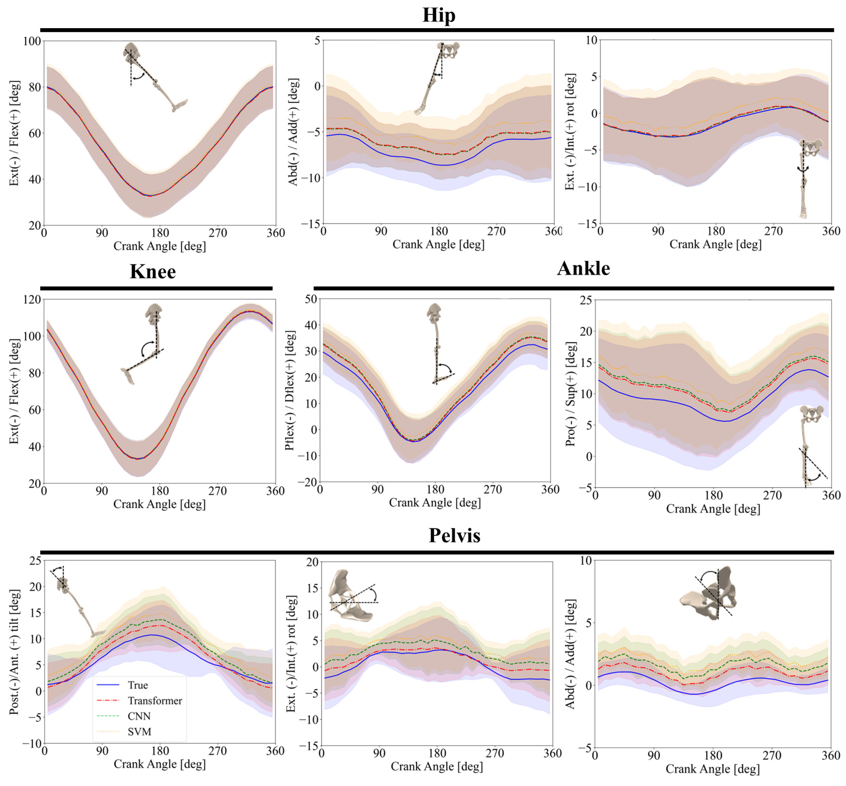
Figure 7 illustrates the inter-subject joint angle predictions over a complete crank revolution for all participants, with each subplot representing a different joint movement. For hip adduction/abduction, predictions from the Transformer model closely followed the reference values throughout the cycle. However, the CNN model exhibited greater errors, particularly within the crank angle ranges of 125–260°, and the SVM model had more than 7° prediction error over the entire cycle. In pelvis adduction/abduction, both the Transformer and CNN models captured the general trend, though with a shift in values. The SVM failed to capture the overall trend accurately, displaying significantly greater errors across the entire cycle. These results suggest that while not flawless, the Transformer and CNN models are more reliable for predicting joint angles during pedaling tasks.

Figure 7. Inter-subject comparison of joint angles predicted by the ML models and those obtained from OpenSim RRA-adjusted kinematics across one crank revolution (mean ± SD). The OpenSim RRA-adjusted reference kinematics are shown as a solid blue line, while the Transformer, CNN, and SVM predictions are distinguished using different line styles (dash–dot, dashed, and dotted, respectively) together with different colors to improve visual discrimination.

Table 5 presents the minimum and maximum joint angles and corresponding ROM values for the OpenSim RRA-adjusted reference kinematics and the predictions from each model in the inter-subject evaluation. Differences from the reference ROM were generally greater than those observed in the intra-subject evaluation. The Transformer generally preserved the reference ROM more closely, while the CNN and SVM showed greater ROM reductions for several joint movements, particularly knee flexion/extension, ankle dorsi/plantar flexion, and subtalar pronation/supination.

Table 5. Minimum and maximum joint angles and corresponding range of motion (ROM) for the OpenSim RRA-adjusted reference kinematics and model predictions in the inter-subject evaluation. All values are reported in degrees.

Joint Movement	Reference Min to Max (ROM)	Transformer Min to Max (ROM)	CNN Min to Max (ROM)	SVM Min to Max (ROM)
Hip flexion/extension	32.1 to 80.3 (48.2)	31.8 to 77.4 (45.6)	34.3 to 75.8 (41.5)	33.2 to 75.1 (41.9)
Hip adduction/abduction	−8.8 to −5.1 (3.7)	−7.9 to −5.0 (2.9)	−8.7 to −2.9 (5.8)	−7.0 to −4.1 (2.9)
Hip internal/external rotation	−3.3 to 0.9 (4.2)	−2.1 to 1.2 (3.3)	−0.4 to 1.3 (1.7)	0.3 to 4.8 (4.5)
Knee flexion/extension	34.7 to 114.8 (80.1)	34.1 to 113.6 (79.5)	37.9 to 111.5 (73.6)	41.6 to 108.2 (66.6)
Ankle dorsi/plantar flexion	−4.4 to 32.6 (37.0)	0.9 to 33.9 (33.0)	2.1 to 33.4 (31.3)	−0.1 to 29.2 (29.3)
Subtalar pronation/supination	5.4 to 13.9 (8.5)	6.7 to 14.1 (7.4)	8.4 to 15.2 (6.8)	7.8 to 12.5 (4.7)
Pelvis anterior/posterior tilt	1.7 to 10.9 (9.2)	1.1 to 12.4 (11.3)	1.5 to 11.3 (9.8)	1.1 to 12.9 (11.8)
Pelvis internal/external rotation	−2.2 to 3.7 (5.9)	−1.1 to 4.1 (5.2)	−2.2 to 4.8 (7.0)	−1.9 to 5.2 (7.1)
Pelvis adduction/abduction	−0.8 to 1.2 (2.0)	1.6 to 3.5 (1.9)	0.9 to 2.9 (2.0)	0.5 to 4.9 (4.4)

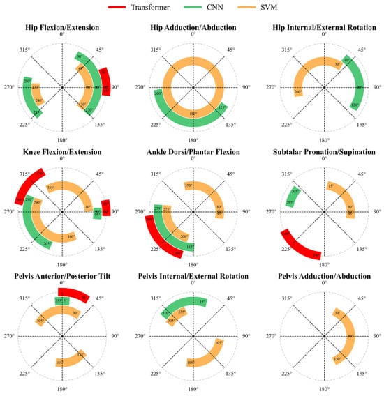
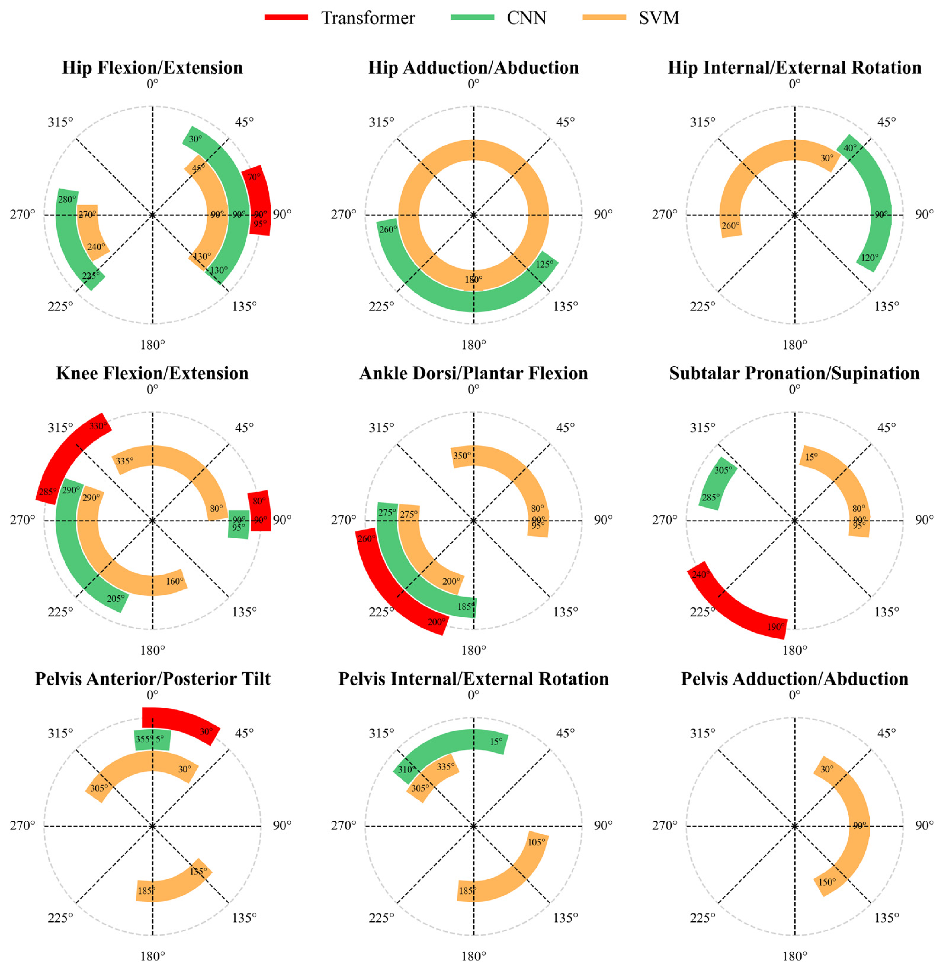
To provide a clearer comparison of model performance across multiple joints, Figure 8 highlights the phases of low performance for each model (Transformer, CNN, and SVM) during the inter-subject evaluation. These low-performance phases were identified based on crank angle ranges where the normalized prediction error exceeded 3% nRMSE. This threshold was selected based on the typical accuracy of laboratory-grade marker-based optical motion capture systems, which exhibit lower-limb kinematic reconstruction errors on the order of 1–2°; a 3% nRMSE threshold represents an approximately equivalent relative tolerance for joints with angular ranges exceeding 30°, and thus distinguishes model errors that exceed the reference-measurement noise floor. It should be noted, however, that relative thresholds impose differential absolute tolerances across joints, approximately 2.1° for hip flexion (range ~70°) but only ~0.21° for hip adduction (range ~7°). A fixed absolute threshold (e.g., 5°) may be considered in future work.

Figure 8. Crank angle ranges associated with low-performance phases during inter-subject comparisons for each ML model. Low-performance phases were identified as crank-angle regions where the normalized prediction error exceeded 3% nRMSE. Colored arcs indicate the affected crank-angle intervals: red for Transformer, green for CNN, and orange for SVM.

The arcs, color-coded in red (Transformer), green (CNN), and orange (SVM), represent the crank-angle regions associated with low predictive performance. The Transformer exhibited only localized low-performance phases, for example during hip flexion/extension (70–95°) and pelvis anterior/posterior tilt (0–30°), suggesting occasional difficulties during biomechanical transitions. The CNN showed low-performance phases primarily in subtalar pronation/supination (285–305°) and knee flexion/extension (90–95° and 205–290°). In contrast, the SVM exhibited more extensive low-performance regions across several joint motions, including hip adduction/abduction (0–360°) and ankle dorsi/plantar flexion (350–95° and 200–275°), indicating greater difficulty in capturing joint kinematics throughout the crank cycle.

4. Discussion

This study compared the performance of SVM, CNN, and Transformer models for predicting lower-limb joint kinematics during stationary cycling using a deployable set of biomechanical and anthropometric input features. An iterative feature-selection process identified a combination of crank angle, pedal angle, cadence, saddle position, body mass, and segment lengths that provided the best predictive performance among the evaluated feature sets. Differences in computational efficiency and prediction accuracy were observed across the three models, emphasizing that model selection should be guided by the intended application.

Two evaluation approaches, intra-subject and inter-subject, were explored. The intra-subject approach aimed for high accuracy by fine-tuning ML models using data from individual participants. This method has potential for enabling personalized monitoring outside the laboratory following an initial data collection session. It could be especially valuable in contexts that demand precise tracking, such as rehabilitation. For instance, data could be collected from patients using instrumented cycling devices equipped with OMC systems. The trained model could then be used to monitor patient progress during rehabilitation on more accessible cycling ergometers. The inter-subject training model, on the other hand, can be applied to new participants even when no subject-specific data are available. This approach offers greater practicality in scenarios requiring real-time monitoring or generalized predictions without prior data collection. Its flexibility makes it especially suitable for clinical and at-home applications, where ease of use and broad applicability are essential for widespread adoption. Importantly, the input features used by the trained models, crank angle, pedal angle, cadence, saddle position, and anthropometrics, can all be measured with commercially available sensors without optical motion capture, making the deployed model suitable for use outside the laboratory. This minimal sensing configuration, comprising a crank encoder, pedal sensors, and a brief anthropometric assessment, represents a practical and cost-effective alternative to laboratory motion capture for monitoring rehabilitation outcomes, training adaptations, or ergonomic assessments in applied settings. However, its prediction accuracy is typically lower than that of an intra-subject model, but this limitation can be partially offset by training on a large and diverse dataset.

Mean ± SD nRMSE values together with omnibus repeated-measures test results, post hoc comparisons, and effect sizes are reported in Table 2 and Table 4, whereas RMSE distributions across participants are shown in Figure 4 and Figure 6. As expected, the intra-subject approach consistently yielded lower error values than the inter-subject approach across all kinematic components, indicating better prediction accuracy when participant-specific data were available for model training. This result indicates that models trained on individualized data are more accurate in predicting joint kinematics for individuals whose data contributed to the training set, highlighting the benefits of personalized data collection for improving prediction precision. In contrast, the greater RMSE and nRMSE values observed in the inter-subject approach underscore the challenges of generalizing predictions across different individuals.

Cycling is a closed-chain activity with lower kinematic variability than open-chain activities such as walking, which is reflected in the smaller standard deviations of some OpenSim RRA-adjusted reference joint trajectories (Figure 5 and Figure 7). Nevertheless, all three models showed larger errors for subtle motions such as hip adduction/abduction, where the total range of motion across a crank cycle was only about 7 degrees (Figure 7).

The frontal-plane pelvis estimates, particularly pelvis adduction/abduction in the inter-subject evaluation, were among the least compelling outputs. This likely reflects the small amplitude of frontal-plane pelvic motion during seated cycling, for which even modest absolute errors represent a large proportion of the total movement range. In addition, pelvis motion in this plane may vary substantially among individuals because of differences in saddle contact, trunk stabilization, and lateral pelvis-control strategies. These subject-specific factors were not directly encoded in the current input set, which included crank angle, pedal angle, cadence, saddle position, anthropometrics, and segment lengths, but not direct measures of pelvis orientation or trunk motion. Future studies may improve frontal-plane pelvis predictions by incorporating pelvis-mounted IMUs, markerless trunk or pelvis features, or other sensors that better capture pelvis–saddle interaction.

Across both intra-subject and inter-subject evaluations, the Transformer produced the lowest prediction errors, the CNN produced slightly higher errors with substantially shorter inference time, and the SVM showed the largest errors overall, particularly in the inter-subject setting. The omnibus and post hoc effect sizes indicate that these differences were not only statistically significant but also practically meaningful across most joint movements. Taken together, the results show a clear trade-off between predictive accuracy and computational efficiency.

These differences can be interpreted in relation to the underlying learning mechanisms of the three models. SVM regression relies on a kernel-based mapping and an epsilon-insensitive margin, which can provide stable performance for moderate nonlinear relationships and relatively small datasets [53]. However, because SVM does not explicitly learn hierarchical temporal features or long-range dependencies, it is less well suited for predicting multi-output kinematic waveforms that vary across participants, saddle positions, and cadence conditions. CNNs improve on this by learning local temporal patterns from consecutive input windows and combining them into higher-level representations [54], which matches the cyclic and locally structured nature of pedaling data and helps explain the favorable balance between accuracy and fast inference time. The Transformer further extends this capability through self-attention, which flexibly models dependencies across the input sequence [43] and likely contributed to its superior generalization, especially in the inter-subject evaluation.

The self-attention mechanism is particularly well suited to a periodic, multi-degree-of-freedom task such as cycling because joint motions are coordinated across repeated crank cycles rather than being determined only by local samples. Self-attention can relate the current phase of one joint to earlier or later phases of the same cycle, and can also capture interdependencies among pelvis, hip, knee, and ankle motions across multiple cycles. This is especially advantageous when cadence, saddle position, or pedaling strategy varies between participants. At the same time, the performance difference between the Transformer and CNN was small for some constrained sagittal-plane movements, such as hip and knee flexion/extension. For these motions, the periodic signal is comparatively regular, and the dominant information is local in time, so the local receptive fields learned by the CNN may already capture most of the relevant structure, reducing the additional benefit of long-range attention.

The results of this study also compare favorably with prior markerless or non-invasive approaches reported for cycling. Although cross-study comparisons should be interpreted cautiously because experimental setups, participant characteristics, cadence protocols, and joint-angle conventions differ, recent cycling studies using OpenCap, and OpenPose reported substantially larger errors for key lower-limb motions [17,61].

Compared with traditional non-ML workflows such as inverse kinematics, the present approach addresses a different practical need. Conventional inverse kinematics can provide anatomically interpretable joint-angle estimates, but it typically depends on optical motion-capture hardware, laboratory calibration, marker placement, and post-processing. In contrast, the present ML framework uses deployable inputs such as crank angle, pedal angle, cadence, saddle position, and anthropometrics to estimate joint kinematics without a full laboratory motion-capture setup. Accordingly, the method is not intended to replace inverse kinematics as a biomechanical reference standard, but rather to provide a more accessible solution for field-based monitoring, rehabilitation, and repeated assessments outside the laboratory.

To facilitate comparison of the evaluated regression models, Table 6 summarizes their prediction performance, computational efficiency, and practical characteristics.

Table 6. Comparison of the prediction performance, computational efficiency, and practical characteristics of the evaluated machine learning regression models.

Model	Intra-Subject RMSE (°)	Inter-Subject RMSE (°)	Inference Time (s) *	Practical Characteristics
Transformer	0.8–1.3	2.7–4.4	~4	Highest prediction accuracy and strongest generalization performance. Suitable for applications where prediction accuracy is prioritized over computational speed.
CNN	0.9–2.4	3.7–6.1	~0.5	Good balance between prediction accuracy and computational efficiency, making it well suited for applications requiring efficient or near real-time deployment.
SVM	1.4–3.4	4.8–7.0	~7	Simple baseline regression model that achieved the lowest prediction accuracy among the evaluated approaches.

* Reported inference times correspond to the total time required to process a 60 s recording on an NVIDIA RTX 5080 GPU.

The findings of the present study should also be considered within the context of recent developments in machine-learning-based biomechanical estimation. Recent studies have demonstrated increasing potential for wearable sensing, deep learning, and Transformer-based architectures to predict lower-limb biomechanical variables across different activities and movement conditions.

Table 7 summarizes recent machine-learning and non-invasive approaches relevant to lower-limb biomechanical estimation and cycling applications. These studies demonstrate a transition from traditional laboratory-based assessments toward more deployable solutions; however, most existing investigations have focused on gait or general locomotor activities rather than cycling-specific applications. Furthermore, direct comparisons among different machine-learning architectures under comparable experimental conditions and evaluation of inter-subject generalization remain limited. The present study contributes to this area by systematically comparing SVM, CNN, and Transformer models for predicting lower-limb joint kinematics during stationary cycling using practical sensor-derived inputs.

Table 7. Comparison of recent machine-learning (ML) and non-invasive approaches for lower-limb biomechanical estimation and cycling applications.

Study	Activity/Input	ML Approach	Predicted Outcomes	Validation/Main Findings	Relevance to Present Study
Moghadam et al. [26]	Walking; IMU + EMG	CNN, RF, SVM, MARS	Lower-limb kinematics, kinetics, and muscle forces	Compared multiple ML approaches under intra- and inter-subject conditions	Demonstrated wearable sensor-based multi-output biomechanical prediction
Sharifi-Renani et al. [49]	Multiple locomotor activities; wearable sensors	Transformer (BioMAT)	Hip, knee, and ankle joint angles	Demonstrated attention-based joint-angle prediction using wearable inputs	Highlighted the potential of Transformer models for biomechanical time-series prediction
Bini et al. [35]	Stationary cycling; markerless video	TransPose, MediaPipe	Hip, knee, and ankle angles	Demonstrated feasibility of low-cost cycling kinematic estimation; accuracy varied across joints	Showed alternative approaches for cycling biomechanics assessment
Hur et al. [47]	Walking; IMU	CNN/LSTM with transfer learning	Lower-limb joint angles	Improved prediction for unseen users using transfer learning	Highlighted personalization and generalization challenges
Cordero-Sánchez et al. [51]	Cycling; lower-limb kinematics	Recurrent neural network	Pedal forces, joint moments, power-related variables	Demonstrated cycling kinetic prediction using ML models	Expanded cycling ML applications beyond kinematic prediction
Torres et al. [52]	Cycling; lower-limb joint kinematics	ANN and regression models	Pedaling performance metrics	Demonstrated prediction of cycling-related variables	Highlighted increasing use of ML in cycling performance analysis
Wang et al. [50]	Lower-limb movement; EMG	Dual Transformer network	Joint angles and joint torques	Simultaneous prediction of kinematic and kinetic variables	Demonstrated recent Transformer-based multimodal biomechanical prediction
Present study	Stationary cycling; crank angle, pedal angle, cadence, saddle position, anthropometrics	SVM, CNN, Transformer	Nine lower-limb joint angles	Compared architectures under intra- and inter-subject conditions	Provides systematic comparison of ML architectures using deployable cycling inputs

Some limitations of the present study also help explain the remaining prediction errors. Cadences ranged from 50 to 80 rpm, which represents the lower range commonly used by trained cyclists and may limit generalization to higher-intensity conditions. In addition, the sample size was modest (N = 15), and the sex distribution was unequal (10 males and 5 females). Consequently, the study was not designed or sufficiently powered to evaluate sex-specific differences in kinematic patterns or model performance, and no sex-stratified analysis was performed. This imbalance may increase the risk of overfitting in the deep learning models and may limit model generalizability to populations with different sex distributions. Although early stopping, dropout, validation-based model selection, and leave-one-subject-out inter-subject evaluation were used to reduce overfitting, the limited and imbalanced dataset remains an important constraint.

Future work should therefore include larger and more diverse cohorts with balanced sex representation, sufficient subgroup sizes for sex-stratified model evaluation, broader age and anthropometric ranges, different cycling experience levels, and clinical populations. Expanding the dataset to include a wider range of cadences, workloads, saddle configurations, and cycling techniques should improve robustness across real-world conditions. Incorporating data from professional cyclists, individuals with musculoskeletal injuries or lower-limb disorders, and additional wearable sensors such as IMUs may further improve generalizability and support more comprehensive biomechanical monitoring.

Finally, while we used a multi-output model to predict ankle, knee, hip and pelvis joint angles simultaneously, this architecture may have affected the accuracy of individual joint angle predictions. Future research could explore single-output models targeting specific joint angles to better understand model behavior and improve prediction accuracy.

The personalized musculoskeletal model used in this study lacked degrees of freedom for knee adduction/abduction and knee internal/external rotation, which limited the examination of these motions and their contributions to overall cycling kinematics. Additionally, variability in data due to differences in equipment, calibration procedures, and marker placement across laboratories could impact the accuracy of joint angle estimations. Incorporating datasets from multiple laboratories into the training process could improve model generalizability and robustness, enabling more comprehensive analyses of joint kinematics during cycling. Addressing these limitations in future research will be essential for refining predictive models and enhancing their applicability across diverse experimental and clinical settings.

5. Conclusions

In this study, we demonstrated that ML techniques could effectively address limitations inherent in traditional biomechanical analysis methods. The results showed that the Transformer model achieved the best overall performance in predicting lower-limb joint kinematics, whereas the CNN model offered a favorable balance between accuracy and computational efficiency. The Transformer and CNN models show strong potential for clinical and exercise applications, with the CNN model being particularly well suited for real-time use because of its short computation time. The successful implementation of these models in a laboratory setting supports the feasibility of monitoring body movement outside clinical environments, where traditional motion capture systems may be unavailable. Future work exploring the integration of wearable sensors and multimodal data sources may further enhance the accuracy and applicability of ML models for joint kinematic prediction. By addressing the limitations of the current study, more robust and comprehensive tools may be developed to improve kinematic prediction and extend these capabilities to kinetic variables, such as joint moments and muscle forces. Because kinetics provide insight into internal loading and joint function, their prediction is important for broader real-world biomechanical applications, especially in sports, rehabilitation, and clinical contexts.

References

- Sommar, J.N.; Johansson, C.; Lövenheim, B.; Schantz, P.; Markstedt, A.; Strömgren, M.; Stigson, H.; Forsberg, B. Overall health impacts of a potential increase in cycle commuting in Stockholm, Sweden. Scand. J. Public Health 2022, 50, 552–564. [Google Scholar] [CrossRef] [Scilit]
- Leirdal, S.; Ettema, G. Pedaling technique and energy cost in cycling. Med. Sci. Sports Exerc. 2011, 43, 701–705. [Google Scholar] [CrossRef] [Scilit]
- Atkinson, G.; Davison, R.; Jeukendrup, A.; Passfield, L. Science and cycling: Current knowledge and future directions for research. J. Sports Sci. 2003, 21, 767–787. [Google Scholar] [CrossRef] [Scilit]
- Yum, H.; Kim, H.; Lee, T.; Park, M.S.; Lee, S.Y. Cycling kinematics in healthy adults for musculoskeletal rehabilitation guidance. BMC Musculoskelet. Disord. 2021, 22, 1044. [Google Scholar] [CrossRef] [Scilit]
- Gatti, A.A.; Keir, P.J.; Noseworthy, M.D.; Beauchamp, M.K.; Maly, M.R. Hip and ankle kinematics are the most important predictors of knee joint loading during bicycling. J. Sci. Med. Sport 2021, 24, 98–104. [Google Scholar] [CrossRef] [Scilit]
- Gatti, A.A.; Keir, P.J.; Noseworthy, M.D.; Beauchamp, M.K.; Maly, M.R. Equations to prescribe bicycle saddle height based on desired joint kinematics and bicycle geometry. Eur. J. Sport Sci. 2022, 22, 344–353. [Google Scholar] [CrossRef] [Scilit]
- Vogl, F.; Schütz, P.; Postolka, B.; List, R.; Taylor, W. Personalised pose estimation from single-plane moving fluoroscope images using deep convolutional neural networks. PLoS ONE 2022, 17, e0270596. [Google Scholar] [CrossRef] [Scilit]
- Postolka, B.; Taylor, W.R.; List, R.; Fucentese, S.F.; Koch, P.P.; Schütz, P. Tibio-femoral kinematics of natural versus replaced knees-A comparison using dynamic video fluoroscopy, Program & Abstracts, ISB 2021. In Proceedings of the XXVIII Congress of the International Society of Biomechanics (ISB), Stockholm, Sweden, 25–29 July 2021; p. A42. [Google Scholar]
- Medina-Mirapeix, F.; Martín-San Agustín, R.; Cánovas-Ambit, G.; García-Vidal, J.A.; Gacto-Sánchez, M.; Escolar-Reina, P. An optoelectronic system for measuring the range of motion in healthy volunteers: A cross-sectional study. Medicina 2019, 55, 516. [Google Scholar] [CrossRef] [Scilit]
- Neri, T.; Testa, R.; Laurendon, L.; Dehon, M.; Putnis, S.; Grasso, S.; Parker, D.A.; Farizon, F.; Philippot, R. Determining the change in length of the anterolateral ligament during knee motion: A three-dimensional optoelectronic analysis. Clin. Biomech. 2019, 62, 86–92. [Google Scholar] [CrossRef] [Scilit]
- Plaza-Bravo, J.M.; Mateo-March, M.; Sanchis-Sanchis, R.; Pérez-Soriano, P.; Zabala, M.; Encarnación-Martínez, A. Validity and reliability of the leomo motion-tracking device based on inertial measurement unit with an optoelectronic camera system for cycling pedaling evaluation. Int. J. Environ. Res. Public Health 2022, 19, 8375. [Google Scholar] [CrossRef] [Scilit]
- Uhlrich, S.D.; Falisse, A.; Kidziński, Ł.; Muccini, J.; Ko, M.; Chaudhari, A.S.; Hicks, J.L.; Delp, S.L. OpenCap: Human movement dynamics from smartphone videos. PLoS Comput. Biol. 2023, 19, e1011462. [Google Scholar] [CrossRef] [Scilit]
- Knippenberg, E.; Verbrugghe, J.; Lamers, I.; Palmaers, S.; Timmermans, A.; Spooren, A. Markerless motion capture systems as training device in neurological rehabilitation: A systematic review of their use, application, target population and efficacy. J. Neuroeng. Rehabil. 2017, 14, 61. [Google Scholar] [CrossRef] [Scilit]
- Nath, T.; Mathis, A.; Chen, A.C.; Patel, A.; Bethge, M.; Mathis, M.W. Using DeepLabCut for 3D markerless pose estimation across species and behaviors. Nat. Protoc. 2019, 14, 2152–2176. [Google Scholar] [CrossRef] [Scilit]
- Outerleys, J.; Mihic, A.; Keller, V.; Laende, E.; Deluzio, K. Markerless motion capture provides repeatable gait outcomes in patients with knee osteoarthritis. J. Biomech. 2024, 168, 112115. [Google Scholar] [CrossRef] [Scilit]
- Cronin, N.J.; Walker, J.; Tucker, C.B.; Nicholson, G.; Cooke, M.; Merlino, S.; Bissas, A. Feasibility of OpenPose markerless motion analysis in a real athletics competition. Front. Sports Act. Living 2024, 5, 1298003. [Google Scholar] [CrossRef] [Scilit]
- Kakavand, R.; Ahmadi, R.; Parsaei, A.; Brent Edwards, W.; Komeili, A. Comparison of kinematics and kinetics between OpenCap and a marker-based motion capture system in cycling. Comput. Biol. Med. 2025, 192, 110295. [Google Scholar] [CrossRef] [Scilit]
- Serrancolí, G.; Bogatikov, P.; Huix, J.P.; Barberà, A.F.; Egea, A.J.S.; Ribé, J.T.; Kanaan-Izquierdo, S.; Susin, A. Marker-Less Monitoring Protocol to Analyze Biomechanical Joint Metrics During Pedaling. IEEE Access 2020, 8, 122782–122790. [Google Scholar] [CrossRef] [Scilit]
- Hu, R.; Diao, Y.; Wang, Y.; Li, G.; He, R.; Ning, Y.; Lou, N.; Li, G.; Zhao, G. Effective evaluation of HGcnMLP method for markerless 3D pose estimation of musculoskeletal diseases patients based on smartphone monocular video. Front. Bioeng. Biotechnol. 2024, 11, 1335251. [Google Scholar] [CrossRef] [Scilit]
- Hatamzadeh, M.; Busé, L.; Turcot, K.; Zory, R. Improved markerless gait kinematics measurement using a biomechanically-aware algorithm with subject-specific geometric modeling. Measurement 2024, 234, 114857. [Google Scholar] [CrossRef] [Scilit]
- Atallah, L.; Lo, B.; King, R.; Yang, G.-Z. Sensor Placement for Activity Detection Using Wearable Accelerometers. In Proceedings of the 2010 International Conference on Body Sensor Networks, Singapore, 7–9 June 2010; pp. 24–29. [Google Scholar] [CrossRef] [Scilit]
- Konak, O.; Wischmann, A.; van De Water, R.; Arnrich, B. A Real-time Human Pose Estimation Approach for Optimal Sensor Placement in Sensor-based Human Activity Recognition. In Proceedings of the 8th International Workshop on Sensor-Based Activity Recognition and Artificial Intelligence; Association for Computing Machinery: New York, NY, USA, 2023. [Google Scholar] [CrossRef] [Scilit]
- Uchida, T.K.; Seth, A. Conclusion or illusion: Quantifying uncertainty in inverse analyses from marker-based motion capture due to errors in marker registration and model scaling. Front. Bioeng. Biotechnol. 2022, 10, 874725. [Google Scholar] [CrossRef] [Scilit]
- Chander, H.; Burch, R.F.; Talegaonkar, P.; Saucier, D.; Luczak, T.; Ball, J.E.; Turner, A.; Arachchige, S.N.K.K.; Carroll, W.; Smith, B.K.; et al. Wearable stretch sensors for human movement monitoring and fall detection in ergonomics. Int. J. Environ. Res. Public Health 2020, 17, 3554. [Google Scholar] [CrossRef] [Scilit]
- Seth, A.; Hicks, J.L.; Uchida, T.K.; Habib, A.; Dembia, C.L.; Dunne, J.J.; Ong, C.F.; Demers, M.S.; Rajagopal, A.; Millard, M.; et al. OpenSim: Simulating musculoskeletal dynamics and neuromuscular control to study human and animal movement. PLoS Comput. Biol. 2018, 14, e1006223. [Google Scholar] [CrossRef] [Scilit]
- Moghadam, S.M.; Yeung, T.; Choisne, J. A comparison of machine learning models’ accuracy in predicting lower-limb joints’ kinematics, kinetics, and muscle forces from wearable sensors. Sci. Rep. 2023, 13, 5046. [Google Scholar] [CrossRef] [Scilit]
- Kianifar, R.; Joukov, V.; Lee, A.; Raina, S.; Kulić, D. Inertial measurement unit-based pose estimation: Analyzing and reducing sensitivity to sensor placement and body measures. J. Rehabil. Assist. Technol. Eng. 2019, 6, 2055668318813455. [Google Scholar] [CrossRef] [Scilit]
- Sharifi Renani, M.; Myers, C.A.; Zandie, R.; Mahoor, M.H.; Davidson, B.S.; Clary, C.W. Deep learning in gait parameter prediction for oa and tka patients wearing imu sensors. Sensors 2020, 20, 5553. [Google Scholar] [CrossRef] [Scilit]
- Yeung, T.; Cantamessa, A.; Kempa-Liehr, A.W.; Besier, T.; Choisne, J. Personalized Machine Learning Approach to Estimating Knee Kinematics Using Only Shank-Mounted IMU. IEEE Sens. J. 2023, 23, 12380–12387. [Google Scholar] [CrossRef] [Scilit]
- Xu, D.; Zhou, H.; Jie, T.; Zhou, Z.; Yuan, Y.; Jemni, M.; Quan, W.; Gao, Z.; Xiang, L.; Gusztav, F.; et al. Data-driven deep learning for predicting ligament fatigue failure risk mechanisms. Int. J. Mech. Sci. 2025, 301, 110519. [Google Scholar] [CrossRef] [Scilit]
- Liew, B.X.W.; Rügamer, D.; Mei, Q.; Altai, Z.; Zhu, X.; Zhai, X.; Cortes, N. Smooth and accurate predictions of joint contact force time-series in gait using over parameterised deep neural networks. Front. Bioeng. Biotechnol. 2023, 11, 1208711. [Google Scholar] [CrossRef] [Scilit]
- Zaroug, A.; Garofolini, A.; Lai, D.T.H.; Mudie, K.; Begg, R. Prediction of gait trajectories based on the Long Short Term Memory neural networks. PLoS ONE 2021, 16, e0255597. [Google Scholar] [CrossRef] [Scilit]
- Cecchini, G.; Lozito, G.M.; Schmid, M.; Conforto, S.; Fulginei, F.R.; Bibbo, D. Neural networks for muscle forces prediction in cycling. Algorithms 2014, 7, 621–634. [Google Scholar] [CrossRef] [Scilit]
- Ahmadi, R.; Rasoulian, S.; Veisari, S.F.; Parsaei, A.; Heidary, H.; Herzog, W.; Komeili, A. A Machine Learning Approach for Predicting Pedaling Force Profile in Cycling. Sensors 2024, 24, 6440. [Google Scholar] [CrossRef] [Scilit]
- Bini, R.R.; Nascimento, V.B.; Nibali, A. Validity of neural networks in determining lower limb kinematics in stationary cycling. Sport. Sci. Health 2024, 20, 127–136. [Google Scholar] [CrossRef] [Scilit]
- Zulkifley, M.A.; Mohamed, N.A.; Zulkifley, N.H. Squat Angle Assessment Through Tracking Body Movements. IEEE Access 2019, 7, 48635–48644. [Google Scholar] [CrossRef] [Scilit]
- Błażkiewicz, M.; Wit, A. Artificial neural network simulation of lower limb joint angles in normal and impaired human gait. Acta Bioeng. Biomech. 2018, 20, 43–49. [Google Scholar] [CrossRef] [Scilit]
- Mundt, M.; Johnson, W.R.; Potthast, W.; Markert, B.; Mian, A.; Alderson, J. A comparison of three neural network approaches for estimating joint angles and moments from inertial measurement units. Sensors 2021, 21, 4535. [Google Scholar] [CrossRef] [Scilit]
- Ahmadi, R.; Mohseni, M.; Arjmand, N. AI-based human whole-body posture-prediction in continuous load reaching/leaving activities. J. Biomech. 2025, 185, 112681. [Google Scholar] [CrossRef] [Scilit]
- Zhao, Q.; Zheng, C.; Liu, M.; Wang, P.; Chen, C. Poseformerv2: Exploring frequency domain for efficient and robust 3d human pose estimation. In Proceedings of the IEEE/CVF Conference on Computer Vision and Pattern Recognition, Vancouver, BC, Canada, 17–24 June 2023; pp. 8877–8886. [Google Scholar]
- Zheng, C.; Zhu, S.; Mendieta, M.; Yang, T.; Chen, C.; Ding, Z. 3d human pose estimation with spatial and temporal transformers. In Proceedings of the IEEE/CVF International Conference on Computer Vision, Montreal, QC, Canada, 10–17 October 2021; pp. 11656–11665. [Google Scholar]
- Zhang, J.; Tu, Z.; Yang, J.; Chen, Y.; Yuan, J. Mixste: Seq2seq mixed spatio-temporal encoder for 3d human pose estimation in video. In Proceedings of the IEEE/CVF Conference on Computer Vision and Pattern Recognition, New Orleans, LA, USA, 18–24 June 2022; pp. 13232–13242. [Google Scholar]
- Vaswani, A.; Shazeer, N.; Parmar, N.; Uszkoreit, J.; Jones, L.; Gomez, A.N.; Kaiser, Ł.; Polosukhin, I. Attention is all you need. In Advances in Neural Information Processing Systems 30, Proceedings of the 31st Conference on Neural Information Processing Systems (NIPS 2017), Long Beach, CA, USA, 4–9 December 2017; NeurIPS Foundation: San Diego, CA, USA, 2017; p. 30. [Google Scholar]
- Liu, S.; Yu, H.; Liao, C.; Li, J.; Lin, W.; Liu, A.X.; Dustdar, S. Pyraformer: Low-complexity pyramidal attention for long-range time series modeling and forecasting. In Proceedings of the International Conference on Learning Representations, Virtual Event, 25–29 April 2022. [Google Scholar]
- Li, S.; Jin, X.; Xuan, Y.; Zhou, X.; Chen, W.; Wang, Y.-X.; Yan, X. Enhancing the locality and breaking the memory bottleneck of transformer on time series forecasting. In Advances in Neural Information Processing Systems 32 (NeurIPS 2019), Proceedings of the 33rd Conference on Neural Information Processing Systems (NeurIPS 2019), Vancouver, BC, Canada 8–14 December 2019; NeurIPS Foundation: San Diego, CA, USA; p. 32.
- Zhou, H.; Zhang, S.; Peng, J.; Zhang, S.; Li, J.; Xiong, H.; Zhang, W. Informer: Beyond efficient transformer for long sequence time-series forecasting. In Proceedings of the AAAI Conference on Artificial Intelligence, Montréal, QC, Canada, 16–23 February 2021; Volume 35, pp. 11106–11115. [Google Scholar]
- Hur, B.; Baek, S.; Kang, I.; Kim, D. Learning based lower limb joint kinematic estimation using open source IMU data. Sci. Rep. 2025, 15, 5287. [Google Scholar] [CrossRef] [Scilit]
- Wang, F.; Liang, W.; Afzal, H.M.R.; Fan, A.; Li, W.; Dai, X.; Liu, S.; Hu, Y.; Li, Z.; Yang, P. Estimation of lower limb joint angles and joint moments during different locomotive activities using the inertial measurement units and a hybrid deep learning model. Sensors 2023, 23, 9039. [Google Scholar] [CrossRef] [Scilit]
- Sharifi-Renani, M.; Mahoor, M.H.; Clary, C.W. Biomat: An open-source biomechanics multi-activity transformer for joint kinematic predictions using wearable sensors. Sensors 2023, 23, 5778. [Google Scholar] [CrossRef] [Scilit]
- Wang, Z.; Chen, C.; Chen, H.; Zhou, Y.; Wang, X.; Wu, X. Dual transformer network for predicting joint angles and torques from multi-channel EMG signals in the lower limbs. IEEE J. Biomed. Health Inf. 2025. early access. [Google Scholar] [CrossRef] [Scilit]
- Cordero-Sánchez, J.; Bini, R.; Serrancolí, G. Validity of recurrent neural networks to predict pedal forces and lower limb kinetics in cycling. J. Biomech. 2025, 183, 112619. [Google Scholar] [CrossRef] [Scilit]
- Torres, A.; Nougarou, F.; Domingue, F. Predicting pedalling metrics based on lower limb joint kinematics. Comput. Methods Biomech. Biomed. Eng. 2025, 28, 2418–2432. [Google Scholar] [CrossRef] [Scilit]
- Smola, A.J.; Schölkopf, B. A tutorial on support vector regression. Stat. Comput. 2004, 14, 199–222. [Google Scholar] [CrossRef] [Scilit]
- LeCun, Y.; Bottou, L.; Bengio, Y.; Haffner, P. Gradient-based learning applied to document recognition. Proc. IEEE 1998, 86, 2278–2324. [Google Scholar] [CrossRef] [Scilit]
- Lai, A.K.M.; Arnold, A.S.; Wakeling, J.M. Why are antagonist muscles co-activated in my simulation? A musculoskeletal model for analysing human locomotor tasks. Ann. Biomed. Eng. 2017, 45, 2762–2774. [Google Scholar] [CrossRef] [Scilit]
- Ehrig, R.M.; Taylor, W.R.; Duda, G.N.; Heller, M.O. A survey of formal methods for determining the centre of rotation of ball joints. J. Biomech. 2006, 39, 2798–2809. [Google Scholar] [CrossRef] [Scilit]
- Harrington, M.E.; Zavatsky, A.B.; Lawson, S.E.M.; Yuan, Z.; Theologis, T.N. Prediction of the hip joint centre in adults, children, and patients with cerebral palsy based on magnetic resonance imaging. J. Biomech. 2007, 40, 595–602. [Google Scholar] [CrossRef] [Scilit]
- Hicks, J.L.; Uchida, T.K.; Seth, A.; Rajagopal, A.; Delp, S.L. Is my model good enough? Best practices for verification and validation of musculoskeletal models and simulations of movement. J. Biomech. Eng. 2015, 137, 020905. [Google Scholar] [CrossRef] [Scilit]
- McGinley, J.L.; Baker, R.; Wolfe, R.; Morris, M.E. The reliability of three-dimensional kinematic gait measurements: A systematic review. Gait Posture 2009, 29, 360–369. [Google Scholar] [CrossRef] [Scilit]
- Banos, O.; Galvez, J.-M.; Damas, M.; Pomares, H.; Rojas, I. Window Size Impact in Human Activity Recognition. Sensors 2014, 14, 6474–6499. [Google Scholar] [CrossRef] [Scilit]
- Bini, R.R.; Serrancoli, G.; Santiago, P.R.P.; Pinto, A.; Moura, F. Criterion validity of neural networks to assess lower limb motion during cycling. J. Sports Sci. 2023, 41, 36–44. [Google Scholar] [CrossRef] [Scilit]
Disclaimer/Publisher’s Note: The statements, opinions and data contained in all publications are solely those of the individual author(s) and contributor(s) and not of MDPI and/or the editor(s). MDPI and/or the editor(s) disclaim responsibility for any injury to people or property resulting from any ideas, methods, instructions or products referred to in the content. |
© 2026 by the authors. Licensee MDPI, Basel, Switzerland. This article is an open access article distributed under the terms and conditions of the Creative Commons Attribution (CC BY) license.