Anthropogenic Amplification of Heat Waves Across CONUS: Quantification, Attribution, and Urban Implications ^†

Abstract

Heat waves and cold snaps affect public health, energy demand, and urban infrastructure, yet separating human influence from natural climate variability remains difficult. We quantify changes in temperature extremes over the contiguous United States (CONUS) using daily climate simulations under natural-only, greenhouse-gas-only, and all-forcings historical scenarios and the future SSP3-7.0 scenario. At each land grid cell, a heat wave is six or more consecutive days with daily maximum temperature above the 99th percentile. In CMIP5 CCSM4 simulations (1950–2005), anthropogenic forcing increases heat wave frequency by 5.02 events per year relative to natural forcing (p = 0.000028), and yields an effective amplification ratio of 3.51 (all-forcing relative to natural-only). The CMIP6 CanESM5 simulations (1950–2014) show the same warm shift, and extending them to 2045 under SSP3-7.0 roughly quintuples the rate of hot day increase (95.5 versus 20.6 days per year) and raises heat wave frequency by 5.66 events per year, with an effective amplification ratio of about 2.72. Both ratios exceed one, but are not directly comparable in magnitude. The largest changes fall on regions and cities growing fast in population from 2000 to 2025, underlining the need for heat mitigation planning in these cities.

1. Introduction

The frequency and severity of temperature extremes matter as much for society as changes in mean climate. Heat waves strain electric grids, raise cooling demand, and drive excess mortality in cities, while cold extremes continue to disrupt infrastructure even in a warming world [1,2]. Climate-model experiments and observational analyses have established that hot extremes, including heat waves, have generally become more frequent and intense, while cold extremes have become less frequent and severe [3]. Detection and attribution studies using observed extreme-temperature indices and multimodel forcing experiments have identified a substantial anthropogenic contribution to these changes at global and continental scales and across many subcontinental regions [4,5]. The IPCC Sixth Assessment Report [6] consequently concluded that human influence is the main contributor to the observed increase in the intensity and frequency of hot extremes and the decrease in cold extremes. Formal detection and attribution methods, in particular, fingerprinting regression, were developed to answer exactly this kind of question and have been applied successfully to precipitation and temperature extremes [7].

Against this established background, the objective of the present study is to examine whether controlled forcing experiments from selected CMIP5 and CMIP6 models produce consistent changes in persistent temperature extremes over the contiguous United States, evaluated using the same percentile-based extreme-event framework. This design provides a model-based assessment of forcing-related heat-extreme amplification and its sensitivity to model generation.

In this study, we use natural-only, greenhouse-gas-only, and all-forcing historical simulations from the Community Climate System Model version 4 (CCSM4) [8] to quantify forcing-related differences in heat waves, cold snaps, hot days, and cold days over CONUS between 1950 and 2005. We then examine whether the direction of these simulated responses is reproduced by corresponding experiments from the newer Canadian Earth System Model version 5 (CanESM5) [9] over 1950–2014. Finally, we extend the CanESM5 all-forcing simulation through 2045 under SSP3-7.0 [10] and conduct an exploratory comparison between simulated grid cell heat wave changes and population growth in major U.S. cities, and discuss what the results imply for urban resilience. Because the analysis does not compare model fingerprints with observations, we interpret the results as contrasts among forced model experiments rather than as formal detection and attribution of observed change.

2. Materials and Methods

2.1. Data

We use daily maximum (tasmax) and daily minimum (tasmin) near-surface air temperature from historical simulations of the Community Climate System Model version 4 (CCSM4) [8], part of the CMIP5 archive, and the Canadian Earth System Model version 5 (CanESM5), part of the CMIP6 archive. The CCSM4 model has a horizontal resolution of 0.9375° (latitude) × 1.25° (longitude), and we analyze the period 1 January 1950 to 31 December 2005 at daily frequency. CanESM5 has a horizontal resolution of approximately 2.8° latitude × 2.8° longitude. We analyze the historical period from 1 January 1950 to 31 December 2014 and the future period from 1 January 2015 to 31 December 2045 at daily frequency. The study domain covers land areas within CONUS, from 24.743° N to 49.345° N and from 124.78° W to 66.95° W. For each model, we selected all grid cells whose latitude and longitude fell within this geographic window and whose land–sea mask classified the grid cell as land. All event counts and trends reported below are aggregated over these land grid cells. CCSM4 and CanESM5 were selected because they provide the natural-only, greenhouse-gas-only, and all-forcing experiments required for a comparable assessment across CMIP5 and CMIP6; CanESM5 also provides an SSP3-7.0 extension for the near-future analysis. One realization was analyzed for each model–experiment combination. Therefore, the results characterize the selected realizations rather than the full model or initial-condition-ensemble spread.

Three historical forcing scenarios and one future scenario are compared:

• nat: Natural forcing only, with solar and volcanic forcing varying in time and greenhouse gases, land use, and aerosols fixed at or cycled over their 1850 values.
• ghg: Greenhouse gas forcing only, with all other forcings fixed at or cycled over 1850 values.
• all: All forcings combined (nat + ghg + land use).
• ssp370: The fully forced ssp370 scenario tracks a high emissions pathway reaching a radiative forcing of 7.0 W/m² by 2100 under the “Regional Rivalry” (SSP3-7.0) narrative, which is defined by high national security focus, low international cooperation, and weak environmental governance [10].

2.2. Definitions of Temperature Extremes

Following Mishra et al. [1], a heat wave is a period during which the daily maximum temperature stays above the empirical 99th percentile for six or more consecutive days [11], and a cold snap is the analogous event below the 1st percentile of daily minimum temperature. Hot days and cold days are individual days beyond the same thresholds. Other studies have used the 97.5th [3] or 95th [2] percentiles for similar purposes. The percentile thresholds were computed at every land grid cell for each scenario over the analysis period, and consecutive-day events were identified per grid cell and calendar year using run-length labeling of threshold exceedances. Because events are identified within calendar years, a cold spell continuing across 31 December–1 January is split in two, which may lead to a slight undercount of cold snaps.

Since our interest is in the effect of anthropogenic forcing, event counts in the all and ghg scenarios were computed against the thresholds of the nat scenario. Any excess of events relative to the nat run can then be read as the contribution of the added forcings.

2.3. Trends and Forcing Experiment Comparisons

For each year, we added up the number of hot days, cold days, heat waves, and cold snaps over all land grid cells of CONUS. We then fitted a straight line to each of these annual counts using ordinary least-squares (OLS) regression; the slope of the line gives the rate of change per year, and the associated p-value quantifies uncertainty under the standard OLS assumptions. Since annual event counts in climate-model simulations can exhibit serial correlation, this formulation may underestimate uncertainty, and the p-values reported below should be interpreted with this caveat in mind. Repeating the same line fit at every grid cell on its own produces maps that show where heat waves and cold snaps are increasing or decreasing. One realization or ensemble member was analyzed for each model forcing combination. Therefore, the fitted coefficients and p-values are conditional on the selected realizations and do not incorporate uncertainty across alternative initial conditions.

Motivated by the regression structure used in fingerprinting studies Min et al. [7], we compare annual heat wave frequency responses across the all-forcing and natural-forcing experiments. Because the response and predictor are both model simulations, and no observational response vector or control-run covariance estimate is included, this calculation is interpreted as a within-model response comparison rather than as formal optimal fingerprinting.

For each year and forcing experiment, we aggregated the number of heat waves over all CONUS land grid cells. Let $C_{s,t}$ denote the resulting annual CONUS heat wave count in year t for experiment s, where s $\in all,nat$. We estimated the response in each experiment using

$$C_{s,t}={\alpha }_s+{\beta }_s(t-t_0)+{\epsilon }_{s,t},s\in \{\mathit{all},\mathit{nat}\}$$

(1)

where $t_0$ is the first year of the analysis period, ${\alpha }_s$ is the intercept, and ${\beta }_s$ is the linear rate of change in the annual aggregated heat wave count. The residual $\epsilon$ represents unresolved interannual variation. It is not interpreted as a complete estimate of internal climate variability because only one realization of each forcing experiment was analyzed. To summarize the relative magnitude of the simulated responses, we define an effective amplification ratio:

$${\beta }_{eff}={\beta }_{all}/{\beta }_{nat}$$

(2)

Values of $bet{a}_{eff}>$ 1 indicate that the heat wave count trend is stronger in the all-forcing simulation than in the natural-only simulation.

2.4. CMIP6 Simulations and Future Scenario

To check whether the CCSM4 results depend on the choice of model generation, the same analysis was applied to CMIP6 simulations of the Canadian Earth System Model version 5 (CanESM5) [9]. The nat and ghg scenarios are taken from the hist-nat and hist-ghg experiments of the Detection and Attribution Model Intercomparison Project (DAMIP) [12], and the all scenario from the CMIP6 historical experiment. The CanESM5 grid is coarser than that of CCSM4, at roughly 2.8° in both latitude and longitude. The analysis period is 1 January 1950 to 31 December 2014, and the study area, land masking, and extreme-event definitions follow Section 2.1, Section 2.2 and Section 2.3. The percentile thresholds were computed from the CanESM5 simulations themselves rather than carried over from CCSM4, since the thresholds describe each model’s own simulated climate and cannot be mixed across models.

For the near future, the CanESM5 SSP3-7.0 simulation [10] was appended to the historical run, giving a continuous daily record through 2045. Hot days and heat waves over 2015–2045 were counted against the thresholds of the historical all scenario, so the future counts read as changes relative to the simulated recent climate. The expected change was then computed at each grid cell as the mean annual count over 2015–2045 minus the mean annual count over 1950–2014.

For the urban comparison, we used the 30 largest U.S. cities by 2025 population. City populations for 2000 and 2025 were taken from the U.S. Census Bureau intercensal estimates [13] and Vintage 2025 estimates [14], and the CanESM5 heat wave and cold snap trends were extracted at the grid cell containing each city. Since one CanESM5 grid cell spans roughly 300 km, some neighboring cities share a cell.

3. Results

3.1. Thresholds Shift to Hotter Regimes in Both Model Generations

Table 1 lists the CONUS-wide thresholds from the CMIP5 CCSM4 and CMIP6 CanESM5 simulations. The absolute values differ between the two models, as expected, since each model has its own simulated climate; what can be compared is the direction of the shifts, and it is the same in both. In CCSM4, the heat wave threshold rises by +0.90 °C under all forcings and +0.64 °C under ghg only, and the cold snap threshold warms by +1.52 and +2.62 °C. In CanESM5, the heat wave threshold rises by +0.67 (all) and +1.69 °C (ghg), and the cold snap threshold by +0.46 and +3.56 °C. In both models, anthropogenic forcing moves both tails of the temperature distribution toward hotter regimes, and the ghg-only heat wave threshold sits above the all-forcings one over much of CONUS, which we attribute to land use change: positive feedbacks of CO₂ concentrations on net primary production and increased precipitation act to lower temperatures in the all simulation [15].

Table 1. Temperature extreme thresholds for CONUS from the CCSM4 (CMIP5, 1950–2005) and CanESM5 (CMIP6, 1950–2014) simulations. Values in parentheses are the shifts relative to the nat scenario of the same model.

Model	Scenario	Heat Wave (°C)	Cold Snap (°C)
CCSM4	nat	37.72	−26.65
CCSM4	ghg	38.36 (+0.64)	−24.03 (+2.62)
CCSM4	all	38.62 (+0.90)	−25.13 (+1.52)
CanESM5	nat	41.45	−29.55
CanESM5	ghg	43.13 (+1.69)	−26.00 (+3.56)
CanESM5	all	42.12 (+0.67)	−29.09 (+0.46)

3.2. Hot Days and Cold Days

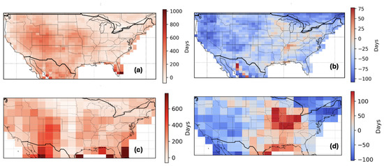
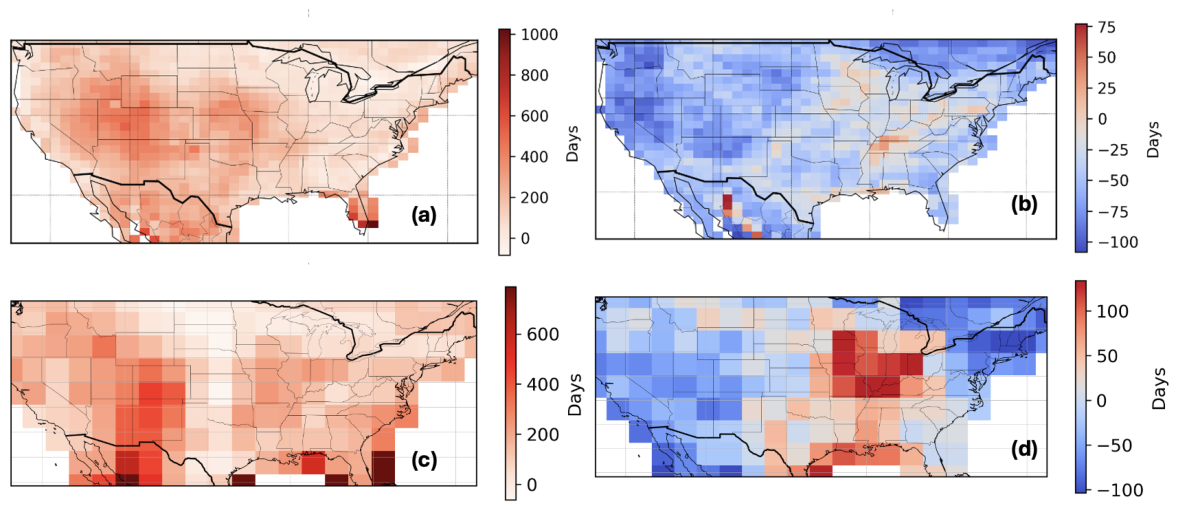
Figure 1 shows where the total number of hot and cold days differs between the all and nat scenarios, counted against the nat thresholds, for both models. The two models paint the same picture. Hot days increase almost everywhere in CONUS, with the largest increases in the West, Southwest, West North Central CONUS, and Florida; cold days decrease at most locations. Aggregated over CONUS in CCSM4, hot days increase at 105.45 days per year (p = 0.0000136), while the decrease in cold days is not statistically significant (−4.00 days per year; p = 0.78). CanESM5 shows the same one-sided behavior, with a highly significant increase in hot days (p ≈ 3 × 10⁻¹¹) and a much weaker cold-day response.

Figure 1. Difference in the total number of hot days (left) and cold days (right) between the all and nat scenarios, using nat thresholds: (a,b) CCSM4, 1950–2005; (c,d) CanESM5, 1950–2014.

3.3. Heat Waves and Attribution

Multi-day events behave like hot days. In CCSM4, heat waves counted against the nat thresholds increase at 5.02 events per year (p = 0.000028) in the all scenario, while cold snaps show no meaningful trend (−0.08 events per year; p = 0.85). CanESM5 agrees: over 1950–2014 it produces 1908 heat waves in the all scenario against 638 under natural forcing alone, roughly a threefold difference, and its heat wave increase is also highly significant (p ≈ 2 × 10⁻⁸).

For CCSM4, the fitted coefficients were ${\beta }_{\mathrm{all}}=71.51$ ($p=1\times {10}^{-7}$) and ${\beta }_{\mathrm{nat}}=20.38$ ($p=0.002$), yielding an effective amplification ratio of

$${\beta }_{\mathrm{eff}}={\displaystyle \frac{{\beta }_{\mathrm{all}}}{{\beta }_{\mathrm{nat}}}}={\displaystyle \frac{71.51}{20.38}}=3.51.$$

Thus, within the selected CCSM4 realizations, the fitted all-forcing coefficient was approximately 3.51 times the natural-only coefficient. The estimated 50-year return level of annual heat wave counts under the all experiment was 971 events yr⁻¹, exceeding the range simulated in the selected natural-only realization.

For CanESM5, the corresponding fitted coefficients were ${\beta }_{\mathrm{all}}=11.79$ ($p\approx 5\times {10}^{-8}$) and ${\beta }_{\mathrm{nat}}=4.34$ ($p\approx 1\times {10}^{-4}$), yielding an effective amplification ratio of

$${\beta }_{\mathrm{eff}}={\displaystyle \frac{{\beta }_{\mathrm{all}}}{{\beta }_{\mathrm{nat}}}}={\displaystyle \frac{11.79}{4.34}}\approx 2.72.$$

Both models therefore produced effective amplification ratios greater than one, indicating a larger fitted response in the all-forcing experiment than in the natural-only experiment. However, these ratios are descriptive of the particular realizations analyzed and do not quantify uncertainty across alternative initial-condition realizations.

3.4. Expected Changes Through 2045 Under SSP3-7.0

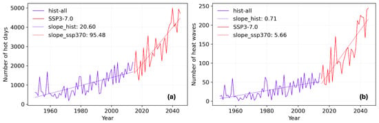
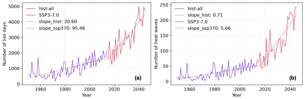
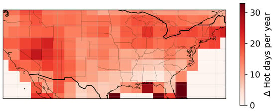
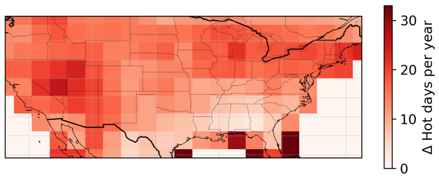
To look ahead, the CanESM5 full forcings run was extended with the SSP3-7.0 scenario and the daily temperatures for 2015–2045 were compared against the historical all-scenario thresholds. Figure 2 shows the annual CONUS totals of hot days and heat waves for the historical period and the future window. Hot days increase at 95.48 days per year over 2015–2045, compared with 20.60 days per year over the historical period, and heat waves increase at 5.66 events per year, against 0.71 per year historically. Figure 3 maps the expected change: the mean annual number of hot days in 2015–2045 minus the mean over 1950–2014. The increase ranges from a few additional hot days per year in the Southeast interior to more than 30 along the Gulf Coast, in Florida, and across the Southwest.

Figure 2. Annual CONUS totals of (a) hot days and (b) heat waves in CanESM5, for the historical all-forcings run (1950–2014) and the SSP3-7.0 continuation (2015–2045), both counted against the historical all-scenario thresholds. Dashed lines show the fitted trends.

Figure 3. Expected change in the annual number of hot days per grid cell: mean over 2015–2045 under SSP3-7.0 minus mean over 1950–2014 in the historical all-forcings run, using historical all-scenario thresholds.

3.5. Temperature Extremes and Urbanization

Climate extremes carry particular weight where people and infrastructure are concentrated [1]. Table 2 lists the nine largest U.S. cities by 2025 population, their growth since 2000, and the CanESM5 heat wave and cold snap trends at the grid cell containing each city. Los Angeles, Phoenix, and San Diego show the strongest heat wave intensification among the nine, and Phoenix combines a strong heat wave trend with the second-fastest growth (+25.5%). Cold snap trends are negative or near zero for almost all cities.

Table 2. Population, growth (2000–2025), and CanESM5 trends of temperature extremes for the nine largest U.S. cities. Trends are the change in the annual number of events per year (all scenario, 1950–2014).

City	Population (2025)	Growth 2000–2025 (%)	Heat Wave Trend	Cold Snap Trend
New York, NY	8,584,629	+7.1	−0.02	−0.08
Los Angeles, CA	3,869,089	+4.5	+1.12	−0.05
Chicago, IL	2,731,585	−5.5	+0.22	−0.17
Houston, TX	2,397,315	+21.4	+0.22	−0.20
Phoenix, AZ	1,665,481	+25.5	+0.91	0.00
Philadelphia, PA	1,574,281	+3.9	+0.08	−0.08
San Antonio, TX	1,548,422	+34.2	+0.15	−0.27
San Diego, CA	1,406,106	+14.5	+0.44	+0.03
Dallas, TX	1,329,491	+11.9	−0.04	−0.15

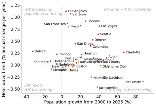
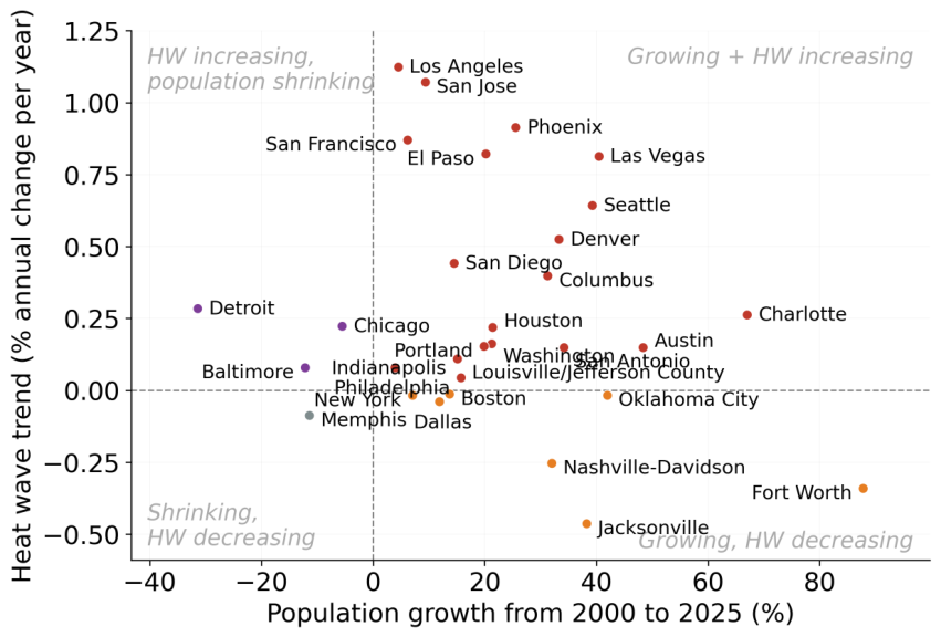
Figure 4 broadens the comparison to the 30 largest cities, placing each by its population growth from 2000 to 2025 and its heat wave trend, with dashed lines at zero splitting the plot into four groups. Nineteen of the 30 cities fall in the upper-right group: population growing and heat waves increasing, which is where adaptation needs compound. The exceptions are the four cities that lost population since 2000 (Chicago, Detroit, Memphis, Baltimore) and seven growing cities where the modeled heat wave trend is flat or negative, including Dallas, Fort Worth, Jacksonville, and Nashville. Since no observed temperatures enter this analysis and the model grid is coarse relative to city scale, we read this as a qualitative screening of where climate and demographic pressures overlap, not a formal attribution.

Figure 4. The 30 largest U.S. cities by 2025 population, placed by population growth (2000–2025, U.S. Census Bureau estimates) and the CanESM5 heat wave trend at the city’s grid cell (all scenario, 1950–2014). Dashed lines mark zero population growth and zero heat wave trend; some neighboring cities share a grid cell.

4. Discussion

The results tell one consistent story. In CCSM4, anthropogenic forcing shifts the extreme-temperature thresholds to hotter regimes, increases hot days and heat waves significantly, and the effective amplification ratio attributes most of the heat wave response to human influence, with a effective amplification ratio of 3.51 over natural only forcing. The CanESM5 simulations, analyzed with the same definitions, show the same threshold shifts and the same one-sided increase in hot extremes, with an amplification of about 2.72 relative to natural forcing, so the finding does not rest on a single model or model generation.

Several observational studies have quantified changes in warm day and heat wave indices over the United States [16,17]. Analyses based on ETCCDI-style indices and U.S. station datasets report significant increases in the frequency of warm days and decreases in cold days over large portions of CONUS, along with more frequent and intense heat extremes in many regions [16,17]. Station-based studies focused on global urban areas also find that most cities have experienced significant increases in the number of heat waves and extreme hot days over the last four decades [1]. Although our hot day metric uses a fixed 99th-percentile threshold and our heat waves are defined from daily maximum temperature in climate-model simulations rather than observations, the sign and spatial pattern of the simulated changes, increased hot days and heat waves over most of CONUS and reduced cold days, are qualitatively consistent with these observational tendencies [1,16].

Under SSP3-7.0, the increase continues and speeds up through 2045. For cities this is a practical concern: more frequent heat waves raise cooling demand and stress interdependent infrastructure networks precisely when they have the least capacity to spare, and several of the fastest growing large cities, led by Phoenix, also face among the strongest heat wave increases. Some caution is warranted: each scenario uses a single model realization, the model grids are coarse relative to city scale, no observed temperatures enter the analysis, and the calendar-year event counting can split winter cold snaps in two. Natural extensions of this work include compound heat–drought events and their spatiotemporal detection [11], larger multimodel CMIP6 ensembles, and coupling with urban energy system models to assess infrastructure vulnerability at the city scale.

The effective amplification ratio is based on one realization of each forcing experiment. Because each realization combines the forced response with a unique trajectory of internal climate variability, the ratio may differ across alternative initial conditions. The analysis therefore does not quantify realization uncertainty, and the reported ratio should be interpreted as descriptive of the selected simulations. Multiple initial-condition members would be required to estimate an ensemble-mean ratio and its uncertainty.

5. Conclusions

Using CCSM4 (CMIP5) simulations for 1950–2005 and CanESM5 (CMIP6) simulations for 1950–2014, each with natural-only, greenhouse-gas-only, and all-forcings scenarios, we quantified changes in simulated temperature extremes over CONUS under different forcing configurations and assessed anthropogenic amplification within the analyzed climate-model experiments. In both models, human influence moves the heat wave and cold snap thresholds to hotter regimes and increases hot days and heat waves; in CCSM4, heat waves increase at 5.02 events per year (p = 0.000028) and the response is amplified by a factor of 3.51 over natural only forcing, while CanESM5 gives an amplification of about 2.72. These simulated increases in hot days and heat waves and decreases in cold days are qualitatively consistent with published observational analyses of warm day and heat wave indices over the United States and global urban areas, although our conclusions remain model-based. This descriptive ratio does not account for uncertainty across alternative initial-condition realizations. Extending CanESM5 with the SSP3-7.0 scenario shows the increase continuing through 2045, with hot days accumulating at nearly five times the historical rate and heat waves increasing at 5.66 events per year. The strongest changes fall on regions and cities that have also grown fastest in population, which places climate-adaptive planning and heat mitigation squarely on the agenda of fast-growing U.S. cities.

References

- Mishra, V.; Ganguly, A.R.; Nijssen, B.; Lettenmaier, D.P. Changes in observed climate extremes in global urban areas. Environ. Res. Lett. 2015, 10, 024005. [Google Scholar] [CrossRef] [Scilit]
- Kodra, E.; Steinhaeuser, K.; Ganguly, A.R. Persisting cold extremes under 21st-century warming scenarios. Geophys. Res. Lett. 2011, 38, L08705. [Google Scholar] [CrossRef] [Scilit]
- Meehl, G.A.; Tebaldi, C. More intense, more frequent, and longer lasting heat waves in the 21st century. Science 2004, 305, 994–997. [Google Scholar] [CrossRef] [Scilit] [PubMed]
- Seong, M.-G.; Min, S.-K.; Kim, Y.-H.; Zhang, X.; Sun, Y. Anthropogenic greenhouse gas and aerosol contributions to extreme temperature changes during 1951–2015. J. Clim. 2021, 34, 857–870. [Google Scholar] [CrossRef] [Scilit]
- Min, S.-K.; Zhang, X.; Zwiers, F.; Shiogama, H.; Tung, Y.-S.; Wehner, M. Multimodel detection and attribution of extreme temperature changes. J. Clim. 2013, 26, 7430–7451. [Google Scholar] [CrossRef] [Scilit]
- Seneviratne, S.I.; Zhang, X.; Adnan, M.; Badi, W.; Dereczynski, C.; Luca, A.D.; Ghosh, S.; Iskandar, I.; Kossin, J.; Lewis, S.; et al. Weather and climate extreme events in a changing climate. In Climate Change 2021: The Physical Science Basis. Contribution of Working Group I to the Sixth Assessment Report of the Intergovernmental Panel on Climate Change; Masson-Delmotte, V., Zhai, P., Pirani, A., Connors, S.L., Péan, C., Berger, S., Caud, N., Chen, Y., Goldfarb, L., Gomis, M.I., et al., Eds.; Cambridge University Press: Cambridge, UK; New York, NY, USA, 2021; pp. 1513–1766. [Google Scholar] [CrossRef] [Scilit]
- Min, S.-K.; Zhang, X.; Zwiers, F.W.; Hegerl, G.C. Human contribution to more-intense precipitation extremes. Nature 2011, 470, 378–381, Erratum in Nature 2013, 498, 526. https://doi.org/10.1038/nature09763.. [Google Scholar] [CrossRef] [Scilit] [PubMed]
- Gent, P.R.; Danabasoglu, G.; Donner, L.J.; Holland, M.M.; Hunke, E.C.; Jayne, S.R.; Lawrence, D.M.; Neale, R.B.; Rasch, P.J.; Vertenstein, M.; et al. The Community Climate System Model version 4. J. Clim. 2011, 24, 4973–4991. [Google Scholar] [CrossRef] [Scilit]
- Swart, N.C.; Cole, J.N.S.; Kharin, V.V.; Lazare, M.; Scinocca, J.F.; Gillett, N.P.; Anstey, J.; Arora, V.; Christian, J.R.; Hanna, S.; et al. The Canadian Earth System Model version 5 (CanESM5.0.3). Geosci. Model Dev. 2019, 12, 4823–4873. [Google Scholar] [CrossRef] [Scilit]
- O’Neill, B.C.; Tebaldi, C.; van Vuuren, D.P.; Eyring, V.; Friedlingstein, P.; Hurtt, G.; Knutti, R.; Kriegler, E.; Lamarque, J.-F.; Lowe, J.; et al. The Scenario Model Intercomparison Project (ScenarioMIP) for CMIP6. Geosci. Model Dev. 2016, 9, 3461–3482. [Google Scholar] [CrossRef] [Scilit]
- Sharma, B.; Kumar, J.; Ganguly, A.R.; Hoffman, F.M. Using image processing techniques to identify and quantify spatiotemporal carbon cycle extremes. In Proceedings of the 2022 IEEE International Conference on Data Mining Workshops (ICDMW), Orlando, FL, USA, 28 November–1 December 2022; pp. 1136–1143. [Google Scholar] [CrossRef] [Scilit]
- Gillett, N.P.; Shiogama, H.; Funke, B.; Hegerl, G.; Knutti, R.; Matthes, K.; Santer, B.D.; Stone, D.; Tebaldi, C. The Detection and Attribution Model Intercomparison Project (DAMIP v1.0) contribution to CMIP6. Geosci. Model Dev. 2016, 9, 3685–3697. [Google Scholar] [CrossRef] [Scilit]
- U.S. Census Bureau. Intercensal Estimates of the Resident Population for Incorporated Places: 2000–2010. Available online: https://www2.census.gov/programs-surveys/popest/datasets/2000-2010/intercensal/cities (accessed on 10 July 2026).
- U.S. Census Bureau. Annual Estimates of the Resident Population for Incorporated Places: Vintage 2025. Available online: https://www2.census.gov/programs-surveys/popest/datasets/2020-2025/cities/totals (accessed on 10 July 2026).
- Sharma, B.; Kumar, J.; Collier, N.; Ganguly, A.R.; Hoffman, F.M. Quantifying carbon cycle extremes and attributing their causes under climate and land use and land cover change from 1850 to 2300. J. Geophys. Res. Biogeosci. 2022, 127, e2021JG006738. [Google Scholar] [CrossRef] [Scilit]
- Mutiibwa, D.; Vavrus, S.J.; Albright, T.P.; McAfee, S.A. Recent spatiotemporal patterns in temperature extremes across the conterminous United States. J. Geophys. Res. Atmos. 2015, 120, 7378–7392. [Google Scholar] [CrossRef] [Scilit]
- Donat, M.G.; Alexander, L.V.; Yang, H.; Durre, I.; Vose, R.; Dunn, R.J.H.; Willett, K.M.; Aguilar, E.; Brunet, M.; Caesar, J.; et al. Updated analyses of temperature and precipitation extreme indices since the beginning of the twentieth century: The HadEX2 dataset. J. Geophys. Res. Atmos. 2013, 118, 2098–2118. [Google Scholar] [CrossRef] [Scilit]
Disclaimer/Publisher’s Note: The statements, opinions and data contained in all publications are solely those of the individual author(s) and contributor(s) and not of MDPI and/or the editor(s). MDPI and/or the editor(s) disclaim responsibility for any injury to people or property resulting from any ideas, methods, instructions or products referred to in the content. |
© 2026 by the authors. Licensee MDPI, Basel, Switzerland. This article is an open access article distributed under the terms and conditions of the Creative Commons Attribution (CC BY) license.