


Abstract
Under the background of urban intensification, the moderating role of green space patterns on Urban Heat Island (UHI) effects has become a significant topic. This study aims to systematically explore the moderating mechanisms of green space patterns on the UHI effect and their spatiotemporal evolution using Nanjing as a case study. We utilized data including the Urban Density Index (UDI), Land Surface Temperature (LST), Green Space Index (GSI), and landscape pattern indices (Patch Density (PD), Largest Patch Index (LPI), and Landscape Shape Index (LSI)) for the years 2012, 2016, and 2020. Pearson correlation analysis, Moran’s I spatial autocorrelation, and a Coupling Coordination Degree Model (CCDM) were employed to quantify these interactions. Urban intensification was associated with a more pronounced UHI effect, as indicated by positive spatial autocorrelation (Moran’s I > 0.4) and a positive correlation between UDI and LST (r = 0.19 in 2020). Conversely, contiguous green spaces demonstrated cooling potential; the correlation between LPI and LST became more negative from r = −0.12 in 2012 to r = −0.25 in 2020, while positive PD-LST correlations were observed in some study years. The spatial mean coupling coordination degree (D) across valid 500 m × 500 m grid cells increased from 0.50 in 2012 to 0.60 in 2020, although coordination in high-density central urban areas remained low (D < 0.3). The fragmentation of green spaces restricts their capacity to regulate urban thermal environments. To optimize green space layout and effectively mitigate the UHI effect, urban planning should prioritize improving green connectivity, expanding contiguous large green areas, and promoting green roofs.
1. Introduction
The accelerating rate of global urbanization has led to rapid increases in urban populations and building density. However, this process has concurrently intensified the Urban Heat Island (UHI) effect, posing a critical challenge to sustainable urban development [1,2]. The UHI effect refers to elevated land surface or atmospheric temperatures in urban areas compared with surrounding non-urban areas, primarily driven by urban densification processes such as surface sealing, anthropogenic heat emissions, and reduced green space coverage [3,4]. The exacerbation of UHI not only increases urban energy consumption and degrades air quality, but also poses threats to public health and urban livability [5,6].
As essential elements of urban ecosystems, urban greenery has a significant impact on alleviating urban thermal anomalies by reducing LST through evapotranspiration, shading, and improved surface albedo [7,8]. However, amid intensifying urban expansion, urban greenery is experiencing growing dispersion, and the evolving patterns in its spatial arrangement and their influence on thermal regulation remain understudied [9,10]. Therefore, examining the temperature-lowering potential of urban greenery configurations amid increasing urban density offers valuable insights for enhancing city design and thermal sustainability [11].
Recent years have witnessed significant advancements in studies on urban greenery and urban thermal anomalies. Multiple studies have confirmed the capacity of green spaces to mitigate thermal anomalies by moderating the microclimate. For instance, Li et al. examined global urban datasets and found that greater green space coverage markedly reduces the prevalence of high-temperature zones in cities [12]. Sun et al. emphasized that the connectivity and morphological features of green spaces have a substantial influence on their cooling capacity, particularly in high-density urban settings [13]. In China, studies have predominantly explored the spatiotemporal evolution of green space configurations and their response to urban heat phenomena. For example, Li et al. utilized multi-temporal data from Nanjing to demonstrate the intensifying impact of urbanization on urban heat phenomenon intensity [14]; Xu et al. evaluated the cooling effects of different green space types in Nanjing and found that wetlands and large parks demonstrate enhanced temperature regulation under extreme heat conditions [15]. Landscape features like patch density and shape complexity have also garnered significant attention. Masoudi et al. revealed that fragmented green spaces diminish cooling performance due to scattered effects, while contiguous green spaces exhibit stronger thermal regulation [16].
Nonetheless, several limitations persist in existing studies. First, although recent studies have begun to explore the multi-dimensional spatial characteristics of green spaces (e.g., area, connectivity, morphology), their complex non-linear coupling relationship with the thermal environment remains insufficiently quantified, particularly under the background of continuous urban intensification. Second, there is limited investigation into the interactions between green space patterns and urban densification variables such as building density and population distribution. Third, some studies overlook spatial heterogeneity in time-series analyses and fail to fully capture the long-term effects of dynamic green space pattern changes on UHIs [17,18,19].
Recent studies have increasingly utilized advanced geospatial techniques to evaluate land use/land cover (LULC) changes and their thermal impacts in rapidly urbanizing cities like Lahore. Tools such as Geospatial Artificial Intelligence (GeoAI) and Google Earth Engine have been effectively employed to quantify land use transitions, confirming strong correlations between green cover reduction and LST increments [20]. The severe decline in urban green spaces over recent decades poses significant challenges to sustainable development goals [21]. Furthermore, predictive models, including CA-Markov and Artificial Neural Networks, have been applied to forecast built-up expansions and subsequent LST variations [22]. Beyond basic coverage metrics, comprehensive ecological evaluations utilizing the Urban Thermal Field Variance Index (UTFVI) [23], alongside multi-dimensional spatial analyses, demonstrate that landscape configuration and composition—particularly fragmentation and shape complexity—significantly dictate LST distributions [24].
Satellite-based observations, spatial analysis, and statistical modeling serve as essential approaches for investigating the relationship between urban greenery and thermal anomalies [25,26]. Satellite-based observation data with high spatial and temporal resolution is widely used to monitor LST and green space distribution. For instance, Yu et al. integrated satellite-based observation data with machine learning techniques to quantitatively analyze the regulatory effects of green space patterns on thermal anomalies [27]. Landscape ecology strategies, such as the use of landscape pattern indices, have been employed to uncover the temporal–spatial evolution of green space structures and their interactions with urban heat conditions [28]. Spatial analytical techniques, including Moran’s I and coupling coordination frameworks, have also been utilized to investigate the spatial associations linking urban greenery and thermal anomalies. Zhou et al., for example, used geographical detectors to identify the influencing factors of green space patterns on thermal anomalies, emphasizing the importance of spatial heterogeneity [29].
Research on this topic spans multiple spatial scales, from global [30] and regional ag-glomerations [31] and individual cities [32] to community-level micro-scales [33]. For instance, Imhoff et al. examined differences in green space distribution and UHI intensity across major global cities [30], while Du et al. analyzed the regional characteristics of green space patterns in the Guangdong–Hong Kong–Macao Greater Bay Area [31]. However, insufficient attention has been paid to the dynamic regulatory mechanisms of green space patterns under varying degrees of urban densification, particularly the lack of multi-temporal and comprehensive assessments for specific cities [34,35].
Despite the progress made, several research gaps remain. Most studies emphasize the role of green space coverage or single-pattern indicators, neglecting in-depth analyses of the comprehensive regulatory mechanisms involving multi-dimensional characteristics such as connectivity, patch density, and shape complexity, and their interaction with urban densification. Furthermore, few studies systematically address the long-term coevolution of green space patterns and UHIs, particularly the evaluation of cooling potential under the framework of the UDI.
Nanjing, a city located in the lower reaches of the Yangtze River in China, offers a representative case for studying the relationship between green spaces and UHIs due to its distinctive geographical setting and rapid urbanization. Its low-lying terrain and strong topographical enclosure hinder heat dispersion, resulting in pronounced summer heat accumulation [36,37]. Additionally, the city’s high population density and intensive building development have contributed to significant urban densification, leading to the fragmentation and functional degradation of green spaces [13,38]. Although initiatives such as green infrastructure development around Purple Mountain and Xuanwu Lake, as well as rooftop greening programs, have been implemented to optimize green space patterns and alleviate the UHI effect, the actual effectiveness and underlying drivers require further investigation [15]. While previous studies have shown correlations between Nanjing’s green space patterns and LST dis-attribution, limited research has explored the regulatory roles of multi-dimensional green space features within the context of urban densification, especially the interaction between green spaces and urban density [13,39].
To bridge these gaps, this study focuses on Nanjing and integrates LST, UDI, GSI, and landscape pattern index data from 2012, 2016, and 2020. Employing Moran’s I spatial autocorrelation analysis, Pearson correlation analysis, and the CCDM, this research systematically investigates the regulatory mechanisms of green space patterns on UHIs under urban densification and their spatiotemporal evolution. The specific objectives are: (1) to analyze the spatiotemporal variations in green space patterns in Nanjing and their association with the UHI effect; (2) to reveal the regulatory effects of multi-dimensional green space characteristics on LST; and (3) to examine the interaction between green space patterns and urban densification indicators and their coupling coordination. This study aims to fill existing research gaps on the dynamic mechanisms and interaction effects of green space patterns, providing empirical evidence and practical references for UHI mitigation and green space optimization in Nanjing and other similar urban contexts.
2. Materials and Methods
2.1. Study Area
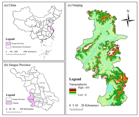
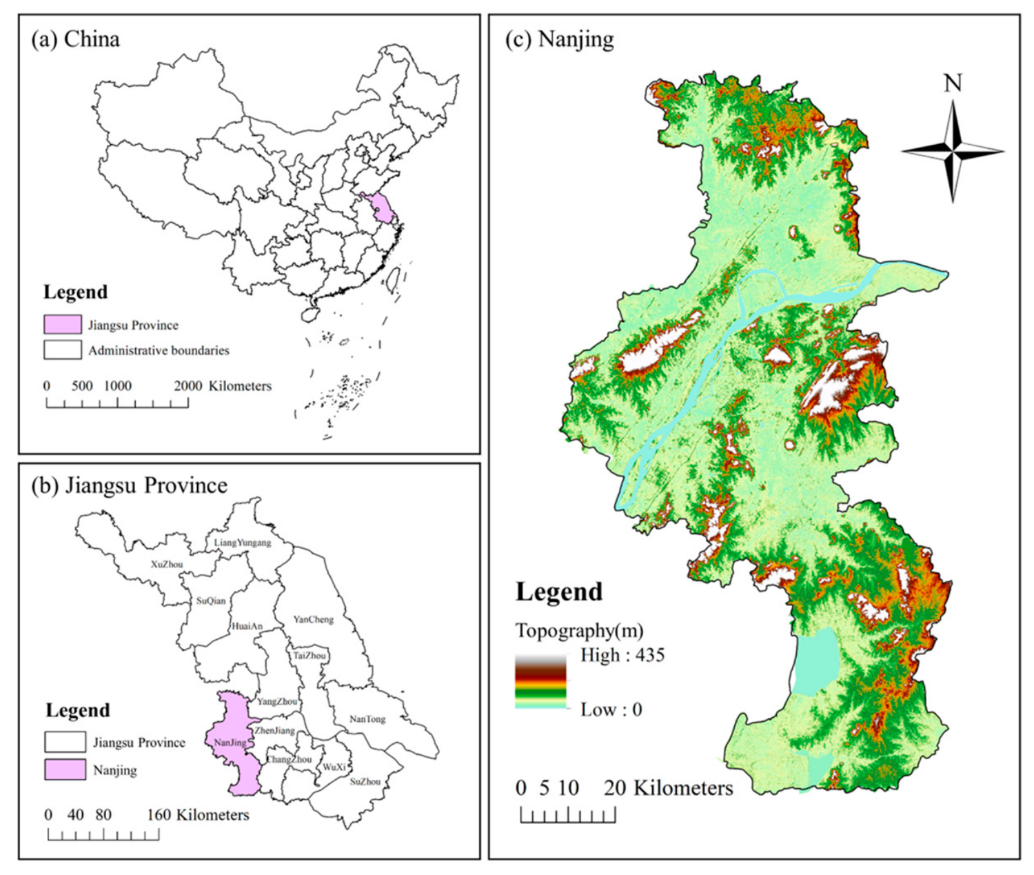
Nanjing, located in the eastern region of Jiangsu Province, China, is a core city within the Yangtze River Delta and plays a pivotal role in regional economic and urban development (Figure 1). In 2020, the city spanned approximately 6587 square kilometers and supported a permanent population exceeding 9.3 million, with over 85% residing in urbanized areas [40,41]. In recent years, Nanjing has undergone rapid urban expansion, characterized by intensified construction activities and significant land use transformations. Nanjing is situated in a subtropical monsoon climate zone, experiencing hot and humid summers as well as cold, damp winters. The city’s annual average temperature is approximately 15.5 °C, and summer temperatures frequently exceed 35 °C [39], contributing to the formation and intensification of the UHI effect. The city boasts a variety of green spaces, including natural reserves such as Zijin Mountain and Xuanwu Lake, as well as an extensive network of urban parks. These green areas account for approximately 30% of the built-up area [42]. However, the ongoing process of urbanization has led to increased fragmentation and reduced connectivity of green spaces. This spatial disintegration has diminished their ecological functionality and weakened their capacity to regulate urban thermal environments. The UHI effect in the central urban area is particularly pronounced, with summer nighttime temperatures observed to be 5–6 °C higher than those in peripheral regions [43]. Therefore, examining the role of green space patterns in mitigating the UHI effect in Nanjing is both scientifically significant and practically valuable for sustainable urban planning and environmental management.
Figure 1.
Study area of Nanjing, China: (a) China; (b) Jiangsu province; (c) topography of Nanjing.
2.2. Data
This study used spatial and environmental input datasets to analyze the UHI effect and green space patterns in Nanjing in 2012, 2016, and 2020. Table 1 summarizes the name, data type, source, and spatial resolution of each externally obtained input dataset. The landscape pattern indices, namely Patch Density (PD), Largest Patch Index (LPI), and Landscape Shape Index (LSI), are not standalone downloaded datasets. Instead, they were derived from green space AOI data at the 500 m × 500 m grid level, as described in Section 2.3.
Table 1.
Description of the spatial and environmental datasets used in this study.
Building vector maps provide detailed information on the location, height, and distribution of urban structures, serving as critical indicators for assessing urban expansion. Floor Area Ratio (FAR) values for Nanjing were calculated using the Baidu building data. Population distribution, LST, and NTL data were integrated to offer a comprehensive perspective on urban growth, facilitating the development of a robust Urban Density Index.
Urban green space AOI data delineate the location, size, and shape of green areas. To analyze spatial distribution patterns, a 500 × 500 m grid was established in ArcGIS 10.8 (Esri, Redlands, CA, USA) across the entire Nanjing municipality. Green space polygons were intersected with the 500 m × 500 m fishnet. When a continuous green space patch crossed one or more grid boundaries, its geometry was clipped at the boundaries, and the portion within each grid cell was treated as a separate within-cell patch. Based on the resulting green space patches within each grid cell, the grid-level landscape pattern indices, including PD, LPI, and LSI, were subsequently calculated. Furthermore, the NDVI, ranging from −1 to 1, is a widely used metric for assessing vegetation health. NDVI values were derived from Landsat remote sensing images processed on the ENVI platform.
2.3. Method
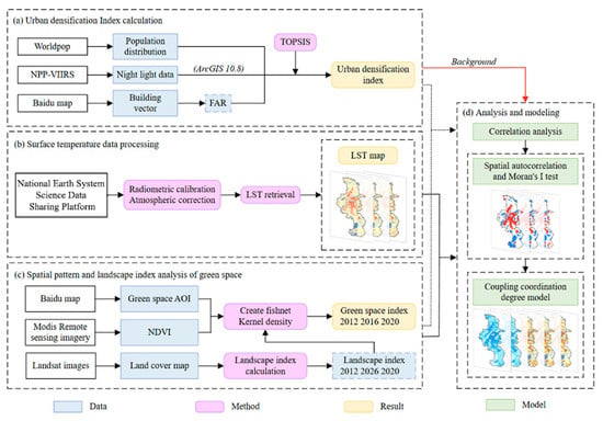
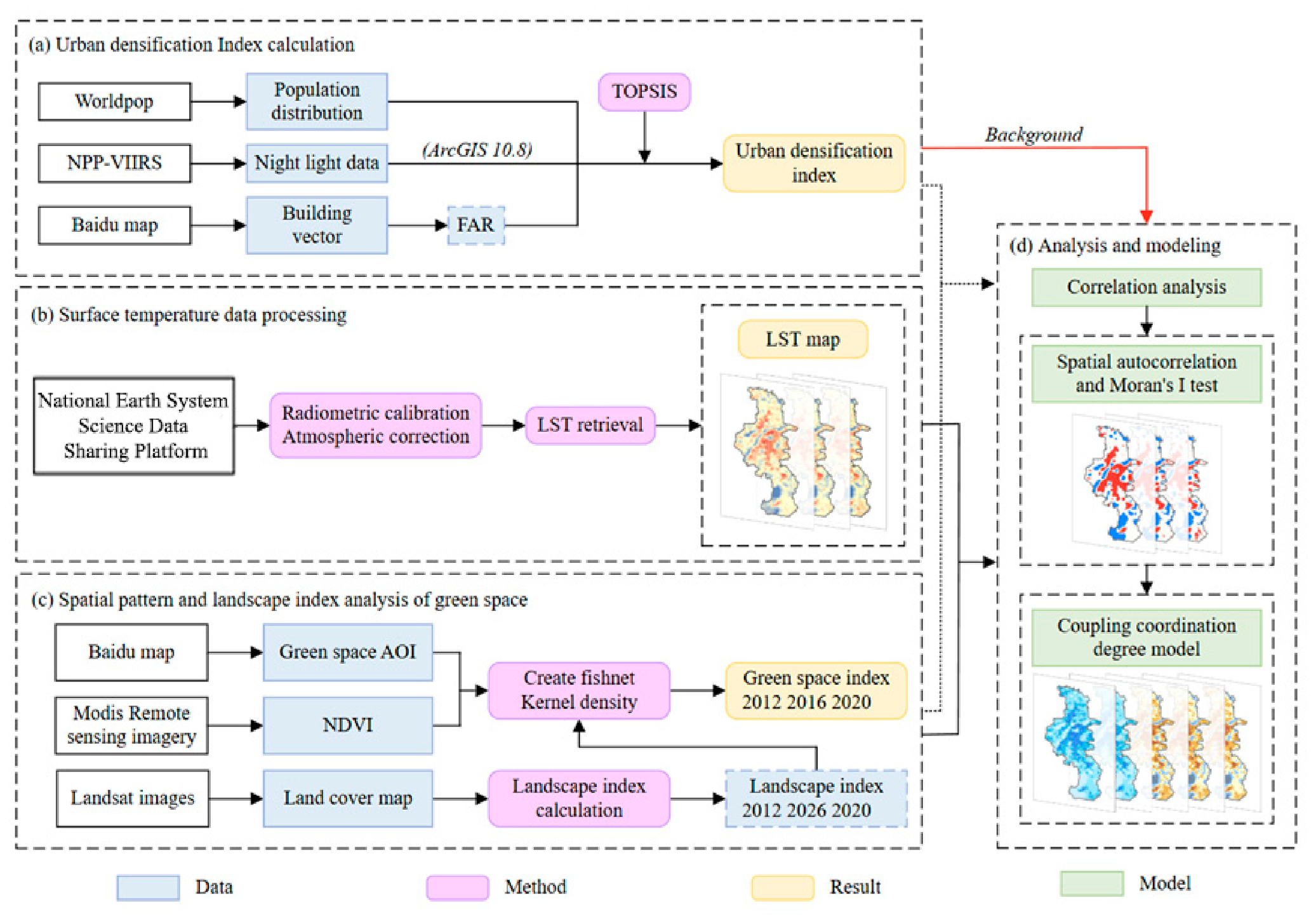
This study consists of four main steps (Figure 2). First, we collect the input data required for the analysis, including building vector data, NTL, population distribution data, LST, green space AOI data, Landsat imagery, and administrative boundary and road data for 2012, 2016, and 2020. The sources and spatial resolutions of these externally obtained input datasets are reported in Table 1. To resolve the spatial scale mismatch between the original 1 km resolution LST data and the 500 m × 500 m analytical grid, a rigorous spatial alignment procedure was conducted in ArcGIS Pro 3.6 (Esri, Redlands, CA, USA). Directly overlaying disparate resolutions can introduce significant modifiable areal unit problem (MAUP) biases. Therefore, the 1 km LST raster was first resampled to a 500 m resolution utilizing the Bilinear Interpolation technique. This algorithm calculates the new pixel value based on a weighted distance average of the four nearest input cell centers, making it highly suitable for continuous environmental surfaces like temperature, as it effectively smooths abrupt transitions [20]. Subsequently, the “Zonal Statistics as Table” tool was employed to calculate the mean LST value for each 500 m × 500 m fishnet grid cell. Concurrently, using the same grid, we derived the UDI, GSI, and landscape pattern indices (PD, LPI, and LSI) for each cell. This ensured that the thermal environment data and all landscape metrics were perfectly aligned within the same spatial analytical unit. Finally, NDVI was derived from Landsat imagery using ENVI.
Figure 2.
Research framework.
Second, the TOPSIS method is applied in ArcGIS 10.8 to calculate the urban densification index, integrating population, night light, and building data (FAR) to generate UDI, capturing urban intensification patterns.
Third, the study looks at how different things like UDI, LST, GSI, NDVI, and landscape measurements are related by using a method called Pearson correlation. It also uses Moran’s I to find clusters of LST and UDI, showing how Urban Heat Islands and green spaces change.
In the end, coupling coordination modeling uses a system called the CCDM to study how green spaces and temperature influence each other. It measures three things: the coupling degree (C), coordination degree (T), and coupling coordination degree (D). These measures help understand how green areas and LST work together in cities, which can guide strategies to reduce the UHI effect.
These phases collectively integrate multi-scale data and analytical methods to uncover the regulatory mechanisms of green space patterns on the UHI in Nanjing.
2.3.1. Pearson Correlation Coefficient
Through correlation analysis, this study explores the relationship between the spatiotemporal patterns of urban green spaces and the UHI effect. Correlation analysis is a statistical method used to determine whether there is an association or relationship between two or more variables. This study utilizes relationship examination to set up the relationship coefficient between green space characteristics within the urban environment (such as scope and region) and indicators of the heat island impact (such as urban temperature contrasts). The Pearson correlation coefficient (r) measures the strength and direction of the linear association between two variables and ranges from −1 to 1. A value of −1 indicates a perfect negative linear correlation, (r = 0) indicates no linear correlation, and a value of 1 indicates a perfect positive linear correlation [48]. The formula for the Pearson correlation coefficient is as follows:
where is the Pearson correlation coefficient; is the th observation of variable x; is the ith observation of variable ; is the mean of variable x; is the mean of variable ; is the number of observations; and indexes the observations from 1 to .
2.3.2. Urban Landscape Indices
PD comes from a scene design file utilized to calculate the thickness of urban green space dissemination and reflects the degree of fracture of green space [49]. If a PD estimation shows a more scattered collection of green spaces and a more prominent level of fracture, this may debilitate their overall cooling impact on the UHI phenomenon [16]. This study analyzes the spatiotemporal changes in PD for green spaces in Nanjing in 2012, 2016, and 2020, and their impacts on LST. PD was calculated separately for each 500 m × 500 m grid cell in ArcGIS 10.8. Green space polygons were intersected with the fishnet, and the clipped patch geometries within each grid cell were used to calculate all landscape metrics. The formula is as follows:
where represents the number of green space patches within an individual grid cell, and A is the area of that grid cell (0.25 km2). Because A is expressed in square kilometers, PD is reported as the number of patches per square kilometer (patches km−2).
The LPI measures the range of the biggest patch inside green spaces, reflecting the contiguity and scale characteristics of the green spaces [49]. A better LPI estimation demonstrates the existence of bigger coterminous ranges inside green spaces. This study calculates the LPI for each year based on the green space AOI information for Nanjing and analyzes the direct impacts of touching green spaces on the LST. The LPI is determined from the range of the biggest patch in the green spaces compared to the entire region, as per the following equation:
where represents the area of the largest patch within the grid cell, are the areas of each green space patch within that cell, and is the area of the individual grid cell (0.25 km2). Max(a1, …, an) and A are both expressed in km2. Therefore, LPI is dimensionless and is reported as a percentage because the ratio is multiplied by 100. The LPI analysis helps reveal how the scale of green spaces influences the UHI effect and provides scientific support for planning contiguous green spaces.
The LSI measures the complexity of the shapes of green spaces, employing a square as the reference benchmark and reflecting the geometric characteristics of the edges of green spaces [44]. A better LSI estimate demonstrates more complex shapes, which may lead to more articulated edge impacts that can affect their regulation of the UHI effect [28]. This study calculates LSI utilizing the green space AOI information for Nanjing, analyzing the effect of green space shape complexity on the LST. The LSI is calculated based on the proportion of the full edge of green spaces to their range, and is standardized according to the following equation:
where is the total perimeter of the green space patch fragments within grid cell , and is the area of grid cell (0.25 km2). The coefficient 0.25 is a geometric normalization factor equal to 1/4, rather than a correction for shape deviations. For a square reference landscape with area , the perimeter is ; therefore, the equation gives for a square landscape. Larger LSI values indicate a greater total edge length relative to the square reference landscape of the same area.
The green space polygons were processed in a projected coordinate system and intersected with the fishnet. Each polygon portion within a grid cell was treated as a within-cell patch fragment. The perimeter was calculated by summing each boundary segment once, including the boundaries formed by the grid-cell extent. Because the calculations were based on vector polygons, no raster four-neighbor or eight-neighbor adjacency rule was applied. Perimeter lengths were converted from meters to kilometers before substitution into the equation, while was expressed in square kilometers; consequently, LSI is dimensionless. In this study, LSI represents the within-cell edge and configuration characteristics of green spaces relative to the grid-cell area, rather than the intrinsic shape complexity of the original un-clipped green space polygons.
LSI analysis can assess the potential impact of green space shapes on the UHI effect and provide references for optimizing green space morphology. Grid cells without green space were excluded from analyses involving PD, LPI, and LSI. Pearson correlation analyses involving these landscape indices were conducted using the corresponding valid grid cells with non-null values for the relevant landscape metric and the corresponding LST observation.
2.3.3. Moran’s I Test
To investigate the spatial designs of urban green spaces in Nanjing, we employ Moran’s I for spatial autocorrelation investigation to recognize and approve spatial clustering or conveyance designs of LST and UDI over distinctive regions [50]. This expository approach is vital for a deeper understanding of the spatiotemporal characteristics of UHIs and their affecting factors [29]. When deciding whether factors display spatial correlation, it is important to portray the spatial dispersion characteristics of biological factors inside a given range. Spatial autocorrelation examination in particular is planned for this reason, essentially improving our understanding of the spatial conveyance designs of LST and their potential driving variables.
The worldwide spatial autocorrelation examination in this study fundamentally depends on Moran’s I. The estimate of Moran’s I ranges from [−1, 1]. When Moran’s I approaches 1, it shows positive spatial autocorrelation, meaning that relationships among spatial units are more tight and comparable values tend to cluster together. On the other hand, when Moran’s I approaches −1, it implies negative spatial autocorrelation, where comparable values are more scattered, and noteworthy contrasts exist among values inside neighborhoods. When Moran’s I approaches 0, it suggests no critical geographic spatial autocorrelation within the data [51]. The equation for Global Moran’s I is as follows:
where n is the number of spatial units; denotes the spatial weight between spatial units i and j, reflecting the spatial proximity relationships; and are the observation values for units i and j, respectively; and is the mean of all observation values across units. The numerator captures the degree of spatial aggregation of similar values by weighted summation of the product of deviations of observations from their mean, weighted by spatial weights, while S2 in the denominator represents the sample variance, which, along with the sum of spatial weights, is used for standardization.
The local Moran’s I calculation formula is as follows:
where is the local autocorrelation index for unit i, and are the observation value for unit i and the global mean, respectively, S2 is the sample variance, and is the spatial weight. This index quantifies the contribution of unit i to the overall spatial pattern by calculating the weighted sum of the products of deviations for unit i and its neighboring units and normalizing by variance. If is significantly positive, it indicates high–high or low–low clustering between unit i and its neighboring units; if significantly negative, it indicates high–low or low–high anomalies [51]. This method effectively pinpoints the core areas of urban heat islands or green space distribution, providing a basis for analyzing spatial heterogeneity.
2.3.4. Coupling Coordination Degree Model
The Coupling Coordination Degree Model (CCDM) has been widely applied to evaluate the interdependence and coordinated development among multiple subsystems [52]. In this study, the CCDM was applied at the 500 m × 500 m grid-cell level to assess the relationship between the thermal-environment subsystem and the green space subsystem under different urban intensification conditions. Specifically, LST and GSI were used as the two CCDM input variables, whereas the landscape pattern indices, including PD, LPI, and LSI, were analyzed separately to interpret the landscape pattern mechanisms underlying the thermal-environment and green space relationship.
The coupling degree (C) reflects the relative balance between the two subsystem scores, whereas the coupling coordination degree (D) jointly considers their interaction and overall development level. Coupling degree alone does not indicate whether the overall system state is desirable, because two equally low subsystem scores may also produce a high coupling degree. Therefore, the comprehensive development index (T) and coupling coordination degree (D) were calculated in addition to (C) [53].
Following the conventional n-system CCDM formulation, the coupling degree is calculated from standardized subsystem scores ranging from 0 to 1 [54]. Because this study includes only two subsystems, namely the thermal-environment subsystem and the green space subsystem, the conventional formulation was reduced to the binary case ( = 2).
Before calculating the CCDM, the raw LST and GSI values for each grid cell were normalized to the range [0, 1] using the Min-Max method [55]. To ensure comparability among 2012, 2016, and 2020, the minimum and maximum values for each variable were derived from the pooled grid-level observations across all three study years. LST was treated as a negative indicator because lower LST represents a more favorable thermal environment, whereas GSI was treated as a positive indicator because higher GSI represents a more favorable green space condition:
where denotes a grid cell; and are the normalized scores of the thermal-environment and green space subsystems, respectively. , , , and are the pooled extrema across all grid cells and study years. Thus, higher values of both and indicate more favorable subsystem conditions.
For the binary system (), the coupling degree was calculated as follows:
where ; a larger indicates a smaller relative disparity between the two subsystem scores. As no theoretical evidence justified assigning unequal importance to the two subsystems, equal weights were used to calculate the comprehensive development index:
where . The coupling coordination degree was then calculated as
where . A larger indicates a more favorable state in which the thermal-environment and green space subsystems are both relatively developed and coordinated. For the exceptional case in which , and were assigned a value of 0 to avoid an undefined ratio.
3. Results
3.1. Spatiotemporal Patterns of Heat Island
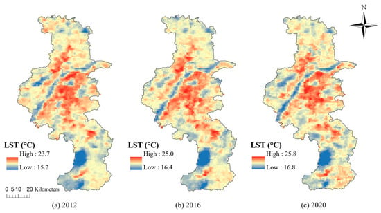
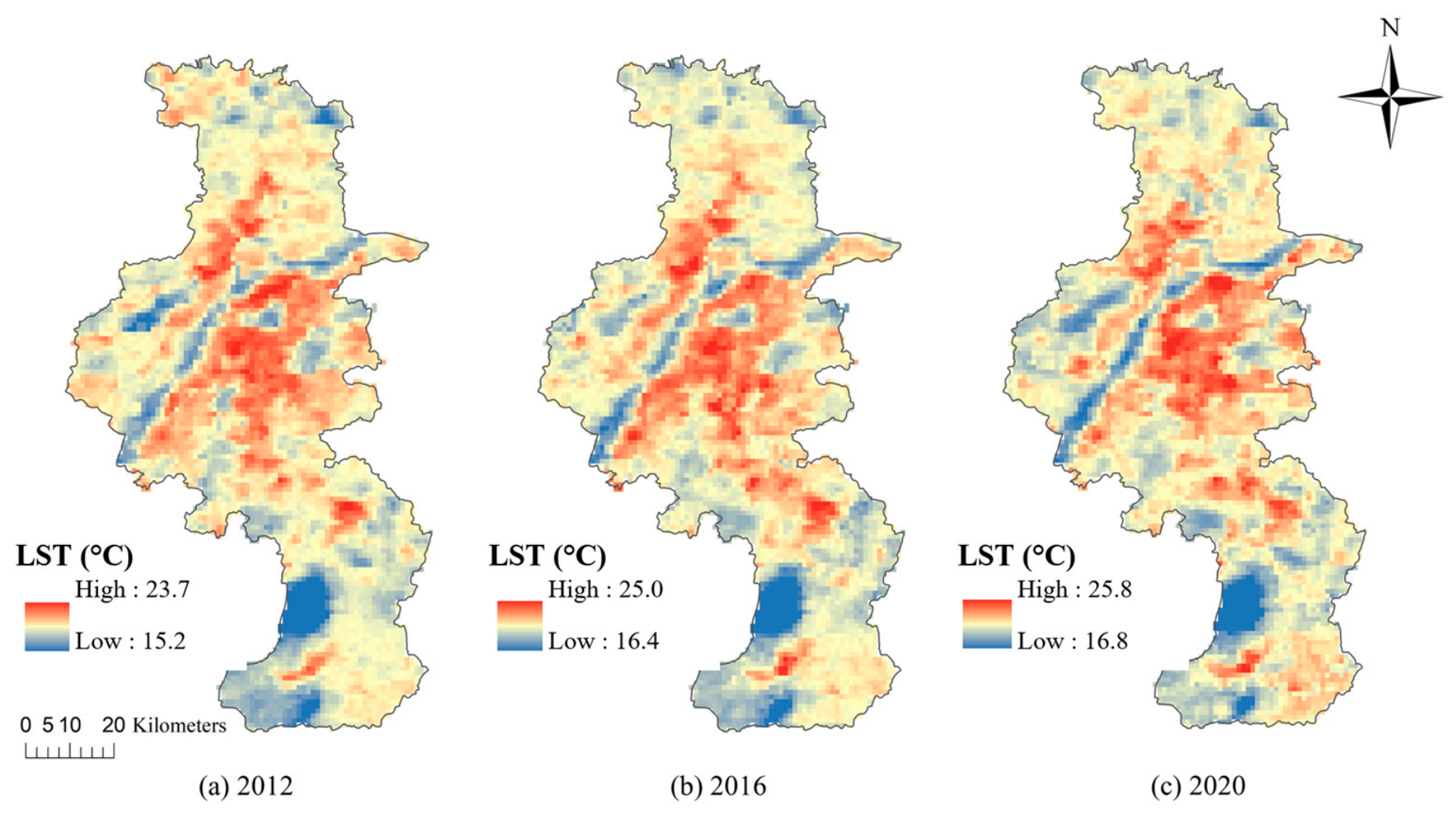
Figure 3 presents the simulated results of the spatial distribution characteristics of LST in Nanjing for 2012, 2016, and 2020. In 2012, the central urban areas, such as Gulou and Xuanwu Districts, exhibited significantly high LST characteristics, with temperatures generally exceeding 32 °C. In contrast, the areas surrounding Mount Zijin and Xuanwu Lake were identified as low-temperature zones, with LST below 28 °C, reflecting the significant cooling effect of green spaces. By 2016, high-temperature regions expanded into the southern new areas, such as Jiangning District, with the area of high-LST zones increasing by approximately 10%, indicating that the urbanization process exacerbated the heat island effect. By 2020, high-temperature areas further expanded, with the proportion of high-LST zones in new areas like Jiangning and Pukou rising to 20%. However, densely green areas, such as Mount Zijin, maintained relatively low temperatures, highlighting the crucial role of green spaces in continuously alleviating the heat island effect.
Figure 3.
Distribution of surface temperature in Nanjing from 2012 to 2020: (a) 2012; (b) 2016; (c) 2020.
The LST in Nanjing showed significant changes across 2012, 2016, and 2020 (Table 2). The Urban Heat Island Intensity (UHII) exhibited a trend of initially decreasing, then increasing, and finally stabilizing, rising to 0.22 by 2012 and remaining stable at about 0.23 thereafter. UHII is calculated as the normalized LST difference between the urban grid and the average rural background temperature. This indicates that the intensity of the UHI effect in Nanjing is gradually stabilizing. During this period, the area of low-temperature zones remained relatively stable, accounting for approximately 6% of the total area, while the area of the next-lowest temperature zones also showed limited change.
Table 2.
Nanjing temperature scale and UHII index table.
3.2. Correlation Matrix Analysis of Green Space Patterns and the Thermal Environment
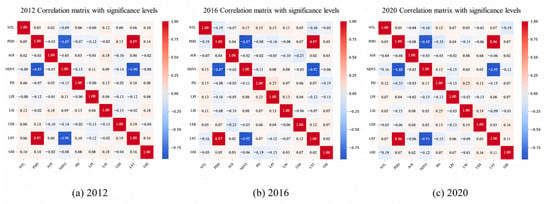
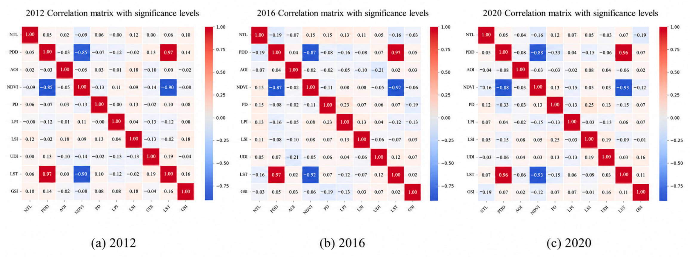
The correlation matrix analysis for Nanjing in 2012, 2016, and 2020 reveals dynamic changes in the relationships among the UDI, LST, GSI, and other landscape pattern indices (Figure 4). In 2012, the correlation coefficient between UDI and LST was 0.19, indicating a positive association between urban density and LST. Meanwhile, the correlation coefficient between UDI and GSI was only −0.04, suggesting that the effect of green space quality on mitigating density was weak. The correlation coefficient of LST with GSI was 0.16, which indicated that areas with lower green space quality exhibited higher temperatures, though the impact was limited. The correlation between NDVI and LST was −0.09, showing a slight cooling effect from vegetation cover, while the correlation between PD and LST was 0.13, indicating that increasing fragmentation of green spaces exacerbated the heat island effect. The correlation coefficient of LPI with LST was −0.12, demonstrating the cooling effect of larger green spaces.
Figure 4.
Correlation coefficient matrix of each index in (a) 2012, (b) 2016, and (c) 2020.
By 2016, the correlation coefficient between UDI and LST had declined to 0.12, while the negative correlation between UDI and GSI strengthened to −0.21, indicating a more pronounced pressure of urban density on green space quality. The correlation coefficient of LST with GSI fell to 0.07, reflecting a decrease in the cooling effect of green spaces. The correlation coefficient for NDVI and LST was −0.16, suggesting an enhanced cooling effect from vegetation, and the correlation between PD and LST shifted to −0.15, implying that the dispersion of green spaces may help alleviate temperatures.
In 2020, the correlation coefficient between UDI and LST rose back to 0.19, while the negative correlation with GSI deepened to −0.13, indicating that urbanization continues to impact green space quality. The correlation of LST with GSI was 0.10, still showing limited regulatory effects of green spaces. The correlation between NDVI and LST became more negative, reaching −0.25, indicating a stronger observed negative association between vegetation and LST. The correlation coefficient of LPI with LST reached −0.25, suggesting that larger green spaces had stronger cooling effects, whereas the correlation between PD and LST was 0.13, indicating that fragmented green spaces once again exacerbated the heat island effect.
3.3. Spatial Autocorrelation Analysis
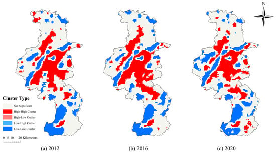
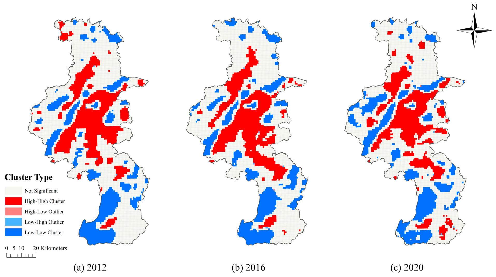
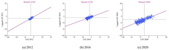
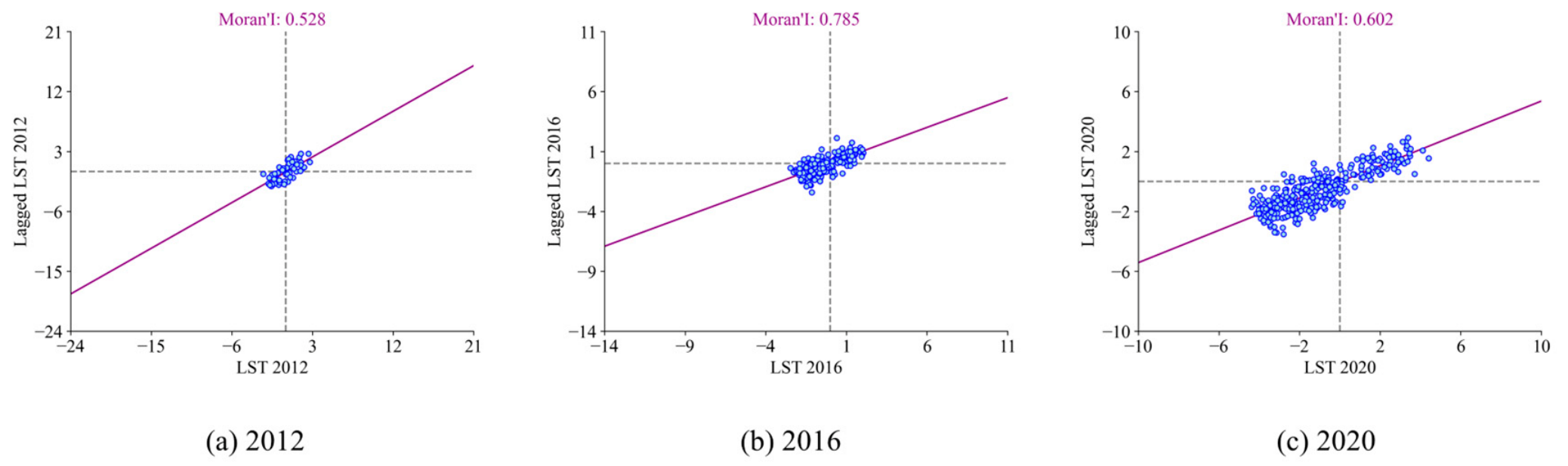
The application of Global Moran’s I is used to understand the spatial autocorrelation of the UDI, LST, and GSI in 2012, 2016, and 2020. The results of the Global Moran’s I (Figure 5 and Figure 6) analysis indicate that in 2012, the high–high (HH) clusters were primarily concentrated in the central urban areas of Nanjing, reflecting a significant UHI effect in the city center. In contrast, low–low (LL) clusters were distributed around green spaces such as Mount Zijin and Xuanwu Lake, demonstrating the cooling effect of green spaces. There were fewer high–low (HL) and low–high (LH) clusters, showing less apparent spatial heterogeneity. By 2016, the HH area expanded southward, encompassing more of the central urban area, indicating an intensification of the UHI effect, while the LL area slightly shrank, suggesting a limited cooling range of green spaces. In 2020, the HH area further expanded into new areas like Jiangning, with the UHI effect continuing to strengthen. The LL area remained concentrated in densely green areas but exhibited a more fragmented distribution.
Figure 5.
Spatial distribution of LST univariate local Moran’s I analysis: (a) 2012, (b) 2016, and (c) 2020.
Figure 6.
Results of LST univariate local Moran’s I cluster analysis: (a) 2012, (b) 2016, and (c) 2020. Blue open circles represent individual grid cells, showing the relationship between LST and its spatial lag. Purple solid lines indicate linear regression fits, and gray dashed lines mark the zero reference values on both axes, dividing each plot into four quadrants.
Table 3 shows the results of the single-variable Global Moran’s I analysis. All the Moran’s I values for UDI, LST, and GSI are positive and are significant. The p-values are all less than 0.001, with z-values over 35, and all of Moran’s indices are greater than 0.4. This indicates a positive spatial autocorrelation between the UDI and urban LST, as well as urban green space quality, allowing for further analysis.
Table 3.
Result of univariate Global Moran’s I.
3.4. Coupling Coordination Between LST and GSI
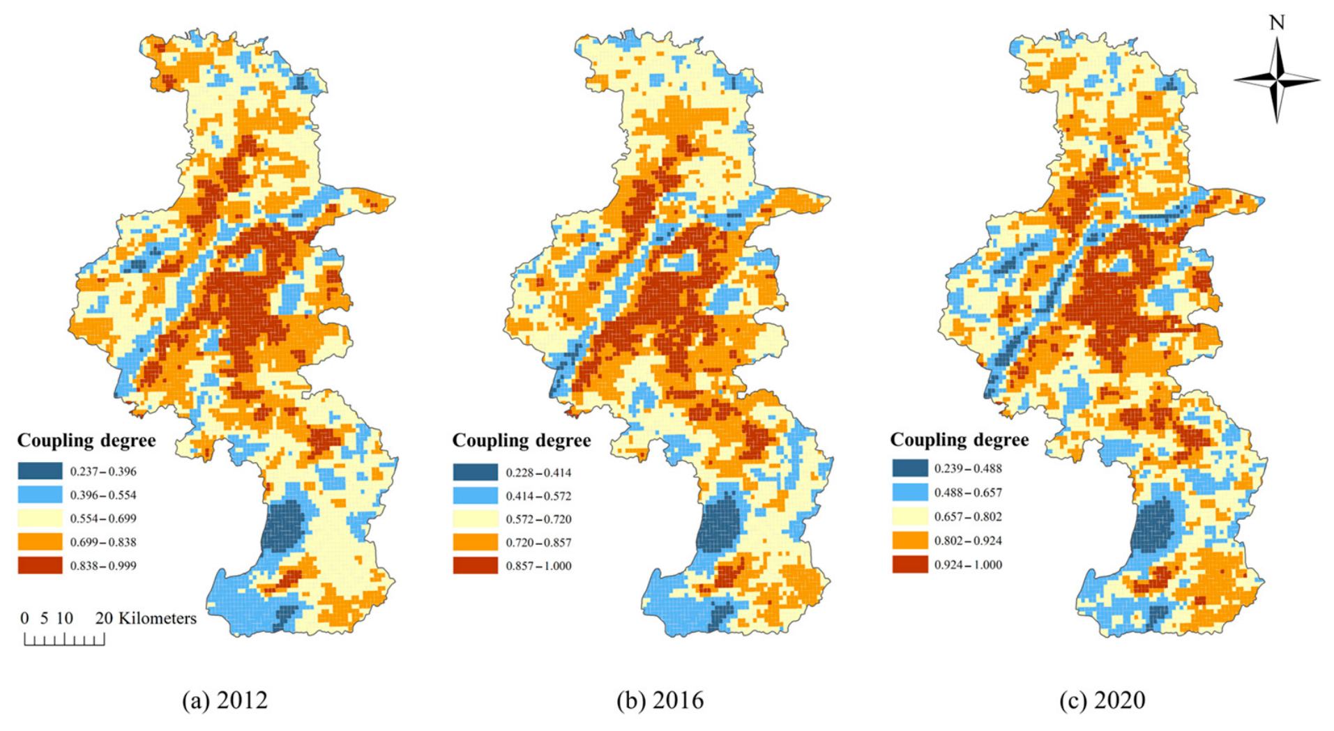
Figure 7 illustrates the spatial coupling characteristics and trends of LST and GSI. In 2012, the coupling degree of LST and GSI indicated that the central urban areas predominantly exhibited high LST and low GSI, suggesting insufficient green spaces in high-density areas, leading to a significant UHI effect. In contrast, areas surrounding Mount Zijin and Xuanwu Lake displayed low LST and high GSI, reflecting the notable cooling effects of green spaces. The distribution of high-coupling-degree regions was limited, primarily situated at the urban periphery, indicating a weak coordination between green spaces and temperature.
Figure 7.
Coupling degree of LST and GSI: (a) 2012, (b) 2016, and (c) 2020.
By 2016, the high LST–low GSI areas expanded southward, signifying that urbanization exacerbated green space loss and temperature increases, with a growing proportion of low-coupling-degree areas. The low LST–high GSI regions slightly diminished, indicating constraints on the cooling range of green spaces, while high-coupling-degree areas remained insignificant. In 2020, the high LST–low GSI regions further expanded, covering more new areas and intensifying the UHI effect. The low LST–high GSI areas remained concentrated in densely green areas but exhibited a more fragmented distribution, with an increase in regions of high coupling degree, suggesting a slight improvement in the coordination between green spaces and temperature in some areas.
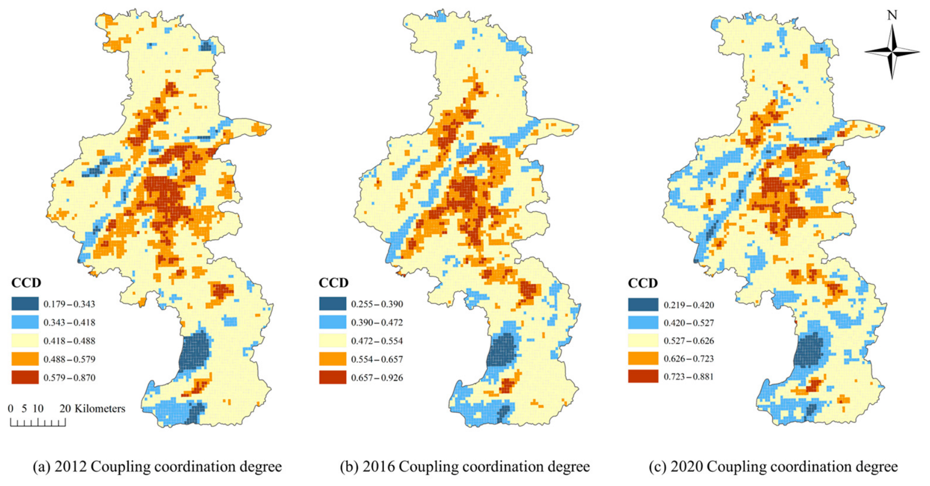
Figure 8 shows a clear trend in the coupling coordination changes between LST and GSI. Low-coupling-coordination areas are primarily concentrated in the central urban areas, reflecting the dislocation between high LST and low GSI and a significant UHI effect. In contrast, high-coordination areas are predominantly located in densely green areas such as Mount Zijin and Xuanwu Lake, where green spaces exert a strong cooling effect. The distribution of moderate-coordination areas is relatively dispersed. Overall, the trend indicates that as urban density increases, the coupling coordination degree between LST and GSI remains low; however, low-coordination areas are gradually decreasing while high-coordination areas are expanding, indicating that the cooling effects of green spaces are increasingly effective in countering UHI growth.
Figure 8.
Coupling coordination degree of LST and GSI: (a) 2012, (b) 2016, and (c) 2020.
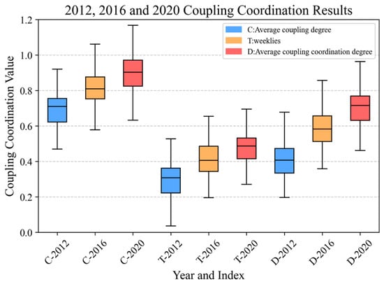
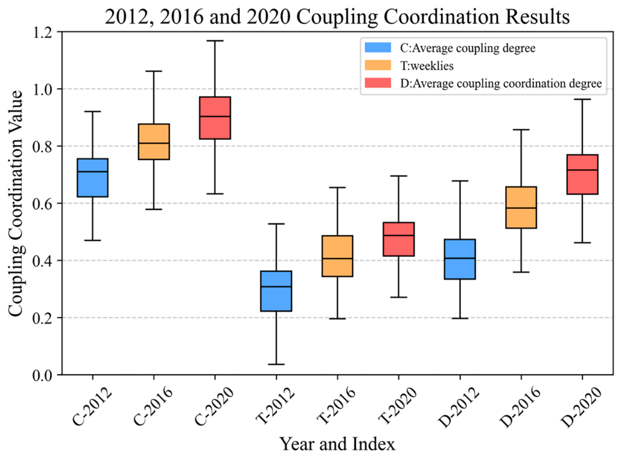
Figure 9 presents the box plots of coupling coordination degree (C), coordination degree (T), and average coupling coordination degree (D) for LST and GSI in Nanjing in 2012, 2016, and 2020. The C values for all three years are around 0.8, showing little fluctuation, indicating a high and stable coupling degree. The T value slightly decreased from 0.6 in 2012 to 0.55 in 2016 but rebounded to 0.6 in 2020, illustrating a trend of initial decrease followed by recovery. The spatial mean of D across valid 500 m × 500 m grid cells increased from 0.50 in 2012 to 0.55 in 2016 and 0.60 in 2020, showing an overall upward trend. This indicates that the coupling coordination degree is gradually improving but still remains at a moderate level (0.5–0.6), suggesting an enhancement in the regulating effects of green spaces on the UHI effect, although there is still considerable room for optimization.
Figure 9.
Coupling coordination change results: (a) 2012, (b) 2016, and (c) 2020.
3.5. Coupling Coordination Between LST and GSI Under Intensification Background
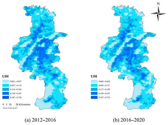
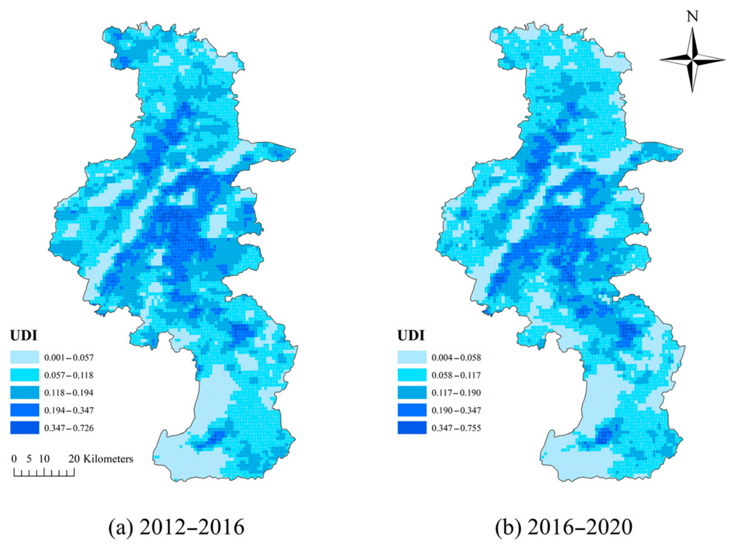
The changes in coupling coordination degree in Nanjing from 2012 to 2016 are displayed (Figure 10). The changes in the central urban area are minimal (0–0.04), indicating a stable coordination between LST and GSI (Figure 11). In contrast, the peripheral new areas show greater changes (0.04–0.08), reflecting the impact of urban expansion on the coordination between green space and temperature. The regions of increased and decreased coupling coordination in the new areas are interspersed, highlighting the complexities of green space layout adjustments.
Figure 10.
Change in coupling coordination degree (D) under urban densification: (a) 2012–2016; (b) 2016–2020.
Figure 11.
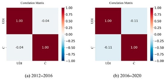
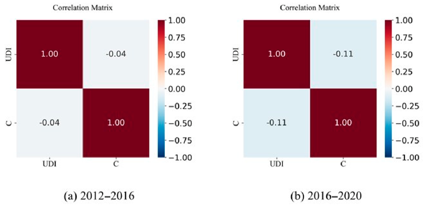
Correlation coefficient between coupling coordination changes and UDI: (a) 2012–2016; (b) 2016–2020.
From 2016 to 2020, the changes in Nanjing’s coupling coordination degree (D) still show minimal variation in the central urban area (0–0.03), indicating that the coordination between LST and GSI remains stable. In the newly expanded urban areas (such as Jiangning and Pukou), however, the changes are significant (0.03–0.11), exhibiting a pattern of interleaved increases and decreases, reflecting the bidirectional impact of urban expansion on the coordination between green space and temperature.
4. Discussion
4.1. Driving Forces of the UHI and the Moderating Effects
The UHI effect refers to the phenomenon where urban areas exhibit significantly higher temperatures than their surrounding rural counterparts. This effect is primarily driven by changes in land use and anthropogenic activities associated with urban expansion. A substantial body of research has demonstrated that increased urban density exacerbates the UHI effect, largely due to the proliferation of impervious surfaces such as roads and buildings, accompanied by a reduction in vegetative cover [56]. For example, an investigation by Akbari et al. within the Journal of Civil Engineering and Management shows that the high heat capacity and high sun-based absorbance of urban building materials are the biggest drivers of the UHI impact, whereas green spaces can lower surface temperatures by 2–4 °C through evapotranspiration and shading effects [57]. Essentially, a survey by Santamouris in Energy and Buildings emphasizes that optimizing green space formats encompasses a noteworthy part in moderating the UHI effect [58].
Current research has some weak points: many studies look at large areas of green spaces and their cooling effects without really examining how the layout of these spaces affects UHI. Also, much of the research uses satellite data and does not check the details on the ground, like how green spaces affect local climates, which hinders the accurate use of their findings. In city management, many local departments have taken steps to reduce the UHI effect. For instance, Singapore encourages bringing greenery to rooftops and tall buildings with its “Garden City” plan, while Tokyo has added more green areas in the city with its “Green Infrastructure” program [33,59]. These actions have successfully lowered city temperatures and improved air quality, giving useful lessons for Nanjing.
This study employs Nanjing as a case study to uncover the regulatory mechanisms of green space spatial patterns on the UHI effect and their spatiotemporal evolution characteristics. It appears that between 2012 and 2020, the high-LST regions in central Nanjing persistently extended, demonstrating profoundly steady positive spatial autocorrelation with the UDI (Moran’s I > 0.4), showing that urban densification may be a major driving force of the exacerbated UHI impact. The GSI showed a low LST–high GSI dissemination design in ranges such as Mount Zijin and Xuanwu Lake, proving the capacity of green spaces to decrease temperatures through evapotranspiration and shading effects. However, the fracture of green spaces within the central urban region (shown by a high PD estimate) limits their cooling run, and the negative relationship between LPI and NDVI (coming to −0.25 in 2020) demonstrates that bordering huge green spaces and established vegetation have a more noteworthy moderation impact on the UHI effect [60]. The coupling coordination degree examination shows that the coupling coordination degree (D estimate) between LST and GSI expanded from 0.5 in 2012 to 0.6 in 2020, suggesting a continuous change within the coordination between green spaces and the warm environment; however, the low coordination degree within the central urban zones (D < 0.3) reflects that the dispersion of green spaces is insufficient to coordinate the concentrated UHI impact in high-density areas [61]. In modern regions (such as Jiangning and Pukou), the changes in coordination degree are critical (extending from 0.03 to 0.11), conceivably related to the expansion and arrangement alterations of green spaces. The relationship between urban densification and changes in coupling coordination degree is weak (−0.11 from 2016 to 2020), indicating that the optimization of green space layouts may be affected by other factors, such as policy interventions and climatic conditions, rather than exclusively determined by urban density. Compared with flat cities such as Shanghai (average coupling coordination degree D ≈ 0.65) [31], the overall coupling coordination level in Nanjing (0.5–0.6) is slightly lower. This difference is mainly attributed to the valley terrain of Nanjing: topographic enclosure hinders heat diffusion, amplifying the UHI intensity in central urban areas and reducing the matching degree between green spaces and the thermal environment.
Moreover, the examination of landscape pattern indices further reveals the intrinsic regulatory mechanisms of green space spatial structure from multiple dimensions. (1) PD: The observed positive association between PD and LST (r = 0.13 in 2020) may reflect two possible mechanisms. First, fragmented green patches may have limited total evapotranspiration capacity per unit area because of their small individual size, reducing their ability to produce sustained cooling effects. Second, scattered patch distributions may interrupt the continuity of cold air flow and weaken the formation of connected cooling corridors, thereby potentially reducing overall thermal-regulation efficiency. (2) LPI: The LPI-LST correlation was negative in both 2012 and 2020 and became more negative from r = −0.12 in 2012 to r = −0.25 in 2020. This observed pattern is consistent with the conclusions of Masoudi et al. [16] and Nasar-u-Minallah et al. [24], who reported that patch scale may influence green space cooling capacity across different climatic zones. This pattern stems from the scale effect of large contiguous green spaces. Large-scale green patches can generate stable regional cold island effects through massive evapotranspiration, and their cooling range can radiate 200–500 m to surrounding built-up areas, forming a gradient cooling zone. With the expansion and protection of core green spaces such as Purple Mountain, the scale cooling effect becomes more prominent over time. (3) LSI: The positive correlation between LSI and LST (r = 0.14 in 2020) indicates that grid cells with greater within-cell green space edge and configuration complexity tended to have higher LST. Given the grid-based calculation using clipped patch fragments, this result should be interpreted as an association with within-cell edge and configuration, rather than as evidence that the intrinsic shape complexity of the original green space polygons alone caused higher LST [62]. Over time, the improvement of green networks in modern regions from 2016 to 2020 has driven the increase in coupling coordination degree, showing the long-term potential of optimized green formats to moderate the UHI effect.
4.2. Coupling Coordination Analysis and Urban Planning Implications
This study not only reveals the moderating mechanisms of green space patterns on the UHI effect under urban intensification but also carries significant theoretical and practical implications. Theoretically, by introducing the CCDM, this study confirms the complex non-linear relationship between urban green space systems and the thermal environment, validating the core role of multi-dimensional spatial characteristics in regulating urban microclimates. This provides empirical support for theoretical research on urban ecosystem services and urban spatial morphology. Practically, these findings offer precise scientific guidance for urban planning: planners should transcend a focus on mere green coverage and prioritize green space connectivity. By expanding contiguous large green patches and curbing the fragmentation of green spaces in high-density areas, cities can enhance their fundamental resilience against heatwaves, providing a viable spatial optimization pathway for achieving sustainable urban development goals.
4.3. Limitations and Future Aspects
However, this study also has certain limitations. Firstly, the research is primarily based on remote sensing data (LST and NDVI) and lacks field measurement data (such as air temperature and humidity) to validate the microclimatic cooling effects of green spaces. This may result in an incomplete understanding of the microclimate regulatory mechanisms. Furthermore, Moran’s I and the CCDM do not adequately account for the spatial heterogeneity of policy factors (such as ecological protection redlines and urban green space planning policies), which may influence the accuracy of the results. In addition, NDVI and LST data are significantly affected by seasonal and meteorological conditions, and thus cannot fully capture the dynamic changes in green space cooling effects.
Future research can be improved in the following ways. First, integrating field measurement data, such as air temperature, humidity, and wind speed, can enhance the validation of the microclimatic cooling mechanisms of green spaces and facilitate the exploration of the combined effects of different green space types, including wetlands, parks, and green corridors. Second, introducing policy variables, such as green space protection regulations and urban planning indicators, can help simulate the impacts of green space patterns across different urban zones, thereby improving the representation of spatial heterogeneity and the predictive accuracy of the analytical models. Third, analyzing multi-temporal data can account for seasonal and meteorological variations, leading to a more refined dynamic assessment of the UHI effect. These improvements will provide a stronger scientific foundation for managing the UHI effect in Nanjing and similar cities, supporting the optimization of green space configurations in urban planning and the development of effective ecological protection strategies.
5. Conclusions
This study conducted a comprehensive spatiotemporal analysis of the UHI effect and green space landscape patterns in Nanjing in 2012, 2016, and 2020. The results demonstrate that urban intensification significantly exacerbates the UHI effect, primarily driven by the expansion of impervious surfaces and the corresponding fragmentation of green spaces. Specifically, the fragmentation of green patches and the increased complexity of their shapes limit their evapotranspiration capacity and cooling range. Conversely, large contiguous green spaces, represented by a higher LPI, exhibit a dominant scale-cooling effect. By introducing the CCDM, this research confirms that while the overall coordination between green spaces and the thermal environment has gradually improved, high-density central urban areas still suffer from severe spatial mismatch. Overall, this study validates the core moderating mechanisms of green space multi-dimensional spatial characteristics (area, connectivity, and morphology) on urban microclimates, providing empirical evidence for the complex non-linear relationship between urban ecosystems and thermal environments.
6. Recommendations
Based on the findings regarding the spatial mismatch and the cooling mechanisms of landscape patterns, the following practical recommendations are proposed for future urban planning and ecological management:
- (1)
- Prioritize Green Space Connectivity: Planners should transcend the traditional focus on mere green coverage rates. It is crucial to construct connected cooling corridors to facilitate cold air flow, thereby expanding the cooling radiation range from suburbs to central high-density areas.
- (2)
- Protect and Expand Core Contiguous Green Patches: Given the dominant cooling role of the Largest Patch Index (LPI), urban renewal projects must strictly protect existing large-scale green spaces and avoid further fragmentation caused by road or building construction.
- (3)
- Implement Micro-Green Infrastructure in High-Density Zones: In central urban areas where land resources are extremely limited, authorities should actively promote 3D greening strategies, such as green roofs and vertical greening, to compensate for the lack of large surface green spaces and alleviate the severe UHI intensity locally.
Author Contributions
Conceptualization, L.S. and G.S.; methodology, L.S. and G.S.; software, L.S. and G.S.; validation, L.S. and G.S.; formal analysis, L.S. and G.S.; investigation, L.S. and G.S.; data curation, L.S. and G.S.; writing—original draft preparation, L.S.; writing—review and editing, L.S. and G.S.; visualization, L.S.; supervision, G.S.; project administration, G.S.; funding acquisition, G.S. All authors have read and agreed to the published version of the manuscript.
Funding
This research was funded by the Open Fund of Key Lab of Natural Resources Monitoring, Department of Natural Resources of Jiangsu Province (Grant No. JSNRM-2025A08); Natural Resources Science and Technology Project of Jiangsu Province (Grant No. JSZRKJ202517); Jiangsu Province Youth Science and Technology Talent Support Project under Grant JSTJ-2025-537; and Science and Technology Project of Xizang Autonomous Region: XZ202601ZY0171.
Institutional Review Board Statement
Not applicable.
Informed Consent Statement
Not applicable.
Data Availability Statement
The data presented in this study are openly available from public repositories. Data is available on request by the corresponding author.
Acknowledgments
We express our thanks to reviewers and editors for their professional comments and suggestions.
Conflicts of Interest
The authors declare no conflicts of interest.
Abbreviations
The following abbreviations are used in this manuscript:
| AOI | Area of Interest |
| CCDM | Coupling Coordination Degree Model |
| FAR | Floor Area Ratio |
| GSI | Green Space Index |
| LPI | Largest Patch Index |
| LSI | Landscape Shape Index |
| LST | Land Surface Temperature |
| NDVI | Normalized Difference Vegetation Index |
| NTL | Nighttime Light |
| PD | Patch Density |
| PDD | Population Distribution Data |
| UDI | Urban Density Index |
| UHI | Urban Heat Island |
References
- Xu, Y.; Zhang, X.; Sun, X.; Wang, J.; Liu, J.; Li, Z.; Guo, Q.; Li, P. Tensile mechanical properties of greenhouse cucumber cane. Int. J. Agric. Biol. Eng. 2016, 9, 1–8. Available online: https://ijabe.org/index.php/ijabe/article/view/1725 (accessed on 23 September 2026).
- Gago, E.J.; Roldan, J.; Pacheco-Torres, R.; Ordóñez, J. The city and urban heat islands: A review of strategies to mitigate adverse effects. Renew. Sustain. Energy Rev. 2013, 25, 749–758. [Google Scholar] [CrossRef] [Scilit]
- Taha, H. Urban climates and heat islands: Albedo, evapotranspiration, and anthropogenic heat. Energy Build. 1997, 25, 99–103. [Google Scholar] [CrossRef] [Scilit]
- Oke, T.R.; Johnson, G.T.; Steyn, D.G.; Watson, I.D. Simulation of surface urban heat islands under ‘ideal’ conditions at night part 2: Diagnosis of causation. Bound.-Layer Meteorol. 1991, 56, 339–358. [Google Scholar] [CrossRef] [Scilit]
- Akbari, H.; Pomerantz, M.; Taha, H. Cool surfaces and shade trees to reduce energy use and improve air quality in urban areas. Sol. Energy 2001, 70, 295–310. [Google Scholar] [CrossRef] [Scilit]
- Yan, H.; Acquah, S.J.; Zhang, J.; Wang, G.; Zhang, C.; Darko, R.O. Overview of modeling techniques for greenhouse microclimate environment and evapotranspiration. Int. J. Agric. Biol. Eng. 2021, 14, 1–8. [Google Scholar] [CrossRef] [Scilit]
- Bowler, D.E.; Buyung-Ali, L.; Knight, T.M.; Pullin, A.S. Urban greening to cool towns and cities: A systematic review of the empirical evidence. Landsc. Urban Plan. 2010, 97, 147–155. [Google Scholar] [CrossRef] [Scilit]
- Yu, Z.; Guo, X.; Jørgensen, G.; Vejre, H. How to cool hot-humid (Asian) cities with urban trees? An optimal landscape size perspective. Agric. For. Meteorol. 2017, 246, 53–64. Available online: https://www.sciencedirect.com/science/article/abs/pii/S0168192318303812?via%3Dihub#references (accessed on 23 September 2026).
- Han, L.; Mao, H.; Kumi, F.; Hu, J. Development of a multi-task robotic transplanting workcell for greenhouse seedlings. Appl. Eng. Agric. 2018, 34, 335–342. [Google Scholar] [CrossRef] [Scilit]
- Li, X.; Zhou, W.; Ouyang, Z.; Xu, W.; Zheng, H. Spatial pattern of greenspace affects land surface temperature: Evidence from the heavily urbanized Beijing metropolitan area, China. Landsc. Ecol. 2012, 27, 887–898. [Google Scholar] [CrossRef] [Scilit]
- Norton, B.A.; Coutts, A.M.; Livesley, S.J.; Harris, R.J.; Hunter, A.M.; Williams, N.S. Planning for cooler cities: A framework to prioritise green infrastructure to mitigate high temperatures in urban landscapes. Landsc. Urban Plan. 2015, 134, 127–138. [Google Scholar] [CrossRef] [Scilit]
- Li, Y.; Svenning, J.-C.; Zhou, W.; Zhu, K.; Abrams, J.F.; Lenton, T.M.; Ripple, W.J.; Yu, Z.; Teng, S.N.; Dunn, R.R.; et al. Green spaces provide substantial but unequal urban cooling globally. Nat. Commun. 2024, 15, 1234. [Google Scholar] [CrossRef] [Scilit] [PubMed]
- Sun, X.; Tan, X.; Chen, K.; Song, S.; Zhu, Z.; Hou, D. Quantifying landscape-metrics impacts on urban green-spaces and water-bodies cooling effect: The study of Nanjing, China. Urban For. Urban Green. 2020, 55, 126838. [Google Scholar] [CrossRef] [Scilit]
- Li, W.; Bai, Y.; Zhou, W.; Han, C.; Han, C. Transformation of Urban Surfaces and Heat Islands in Nanjing during 1984–2018. Sustainability 2020, 12, 6521. [Google Scholar] [CrossRef] [Scilit]
- Xu, H.; Sheng, K.; Gao, J. Mitigation of heat island effect by green stormwater infrastructure: A comparative study between two diverse green spaces in Nanjing. Front. Ecol. Evol. 2023, 11, 1307756. [Google Scholar] [CrossRef] [Scilit]
- Masoudi, M.; Tan, P.Y. Multi-year comparison of the effects of spatial pattern of urban green spaces on urban land surface temperatures. Landsc. Urban Plan. 2019, 184, 44–58. [Google Scholar] [CrossRef] [Scilit]
- Gunawardena, K.R.; Wells, M.J.; Kershaw, T. Utilising green and bluespace to mitigate urban heat island intensity. Sci. Total Environ. 2017, 584, 1040–1055. [Google Scholar] [CrossRef] [Scilit] [PubMed]
- Zhou, W.; Pickett, S.T.; Cadenasso, M.L. Shifting concepts of urban spatial heterogeneity and their implications for sustainability. Landsc. Ecol. 2017, 32, 15–30. [Google Scholar] [CrossRef] [Scilit]
- Estoque, R.C.; Murayama, Y.; Myint, S.W. Effects of landscape composition and pattern on land surface temperature: An urban heat island study in the megacities of Southeast Asia. Sci. Total Environ. 2017, 577, 349–359. [Google Scholar] [CrossRef] [Scilit] [PubMed]
- Sattar, T.; Mirza, N.F.; Javed, M.A.; Nasar-u-Minallah, M.; Malik, S. Changing pattern of urban landscape and its impact on thermal environment of Lahore; Implications for climate change and sustainable development. Environ. Monit. Assess. 2025, 197, 151. [Google Scholar] [CrossRef] [Scilit] [PubMed]
- Azhar, R.; Javed, M.A.; Nasar-u-Minallah, M.; Machado, S.; Jabbar, M. Urban transformation in Lahore: Three decades of land cover changes, green space decline, and sustainable development challenges. Geogr. Environ. Sustain. 2024, 17, 6–17. [Google Scholar] [CrossRef] [Scilit]
- Jabbar, M.; Nasar-u-Minallah, M.; Yusoff, M.M. Predicting the Impact of Land Use Changes on Thermal Environment in Lahore, Pakistan: Implications for Urban Planning. Geogr. Environ. Sustain. 2024, 17, 95–109. [Google Scholar] [CrossRef] [Scilit]
- Nasar-u-Minallah, M.; Haase, D.; Qureshi, S.; Zia, S.; Fatima, M. Ecological monitoring of urban thermal field variance index and determining the surface urban heat island effects in Lahore, Pakistan. Environ. Monit. Assess. 2023, 195, 1212. [Google Scholar] [CrossRef] [Scilit] [PubMed]
- Nasar-u-Minallah, M.; Haase, D.; Qureshi, S. Evaluating the impact of landscape configuration, patterns and composition on land surface temperature: An urban heat island study in the Megacity Lahore, Pakistan. Environ. Monit. Assess. 2024, 196, 627. [Google Scholar] [CrossRef] [Scilit] [PubMed]
- Weng, Q.; Lu, D.; Schubring, J. Estimation of land surface temperature–vegetation abundance relationship for urban heat island studies. Remote Sens. Environ. 2004, 89, 467–483. [Google Scholar] [CrossRef] [Scilit]
- Yan, T.; Zhu, H.; Sun, L.; Wang, X.; Ling, P. Investigation of an experimental laser sensor-guided spray control system for greenhouse variable-rate applications. Trans. ASABE 2019, 62, 899–911. [Google Scholar] [CrossRef] [Scilit]
- Yu, Z.; Yang, G.; Zuo, S.; Jørgensen, G.; Koga, M.; Vejre, H. Critical review on the cooling effect of urban blue-green space: A threshold-size perspective. Urban For. Urban Green. 2020, 49, 126630. [Google Scholar] [CrossRef] [Scilit]
- Connors, J.P.; Galletti, C.S.; Chow, W.T. Landscape configuration and urban heat island effects: Assessing the relationship between landscape characteristics and land surface temperature in Phoenix, Arizona. Landsc. Ecol. 2013, 28, 271–283. [Google Scholar] [CrossRef] [Scilit]
- Zhou, D.; Bonafoni, S.; Zhang, L.; Wang, R. Remote sensing of the urban heat island effect in a highly populated urban agglomeration area in East China. Sci. Total Environ. 2018, 628–629, 415–429. [Google Scholar] [CrossRef] [Scilit] [PubMed]
- Imhoff, M.L.; Zhang, P.; Wolfe, R.E.; Bounoua, L. Remote sensing of the urban heat island effect across biomes in the continental USA. Remote Sens. Environ. 2010, 114, 504–513. [Google Scholar] [CrossRef] [Scilit]
- Du, H.; Cai, Y.; Zhou, F.; Jiang, H.; Jiang, W.; Xu, Y. Urban blue-green space planning based on thermal environment simulation: A case study of Shanghai, China. Ecol. Indic. 2019, 106, 105501. [Google Scholar] [CrossRef] [Scilit]
- Xu, D.; Wang, Y.; Zhou, D.; Wang, Y.; Zhang, Q.; Yang, Y. Influences of urban spatial factors on surface urban heat island effect and its spatial heterogeneity: A case study of Xi’an. Build. Environ. 2024, 248, 111072. [Google Scholar] [CrossRef] [Scilit]
- Hamada, S.; Ohta, T. Seasonal variations in the cooling effect of urban green areas on surrounding urban areas. Urban For. Urban Green. 2010, 9, 15–24. [Google Scholar] [CrossRef] [Scilit]
- Kumar, P.; Debele, S.E.; Khalili, S.; Halios, C.H.; Sahani, J.; Aghamohammadi, N.; Andrade, M.d.F.; Athanassiadou, M.; Bhui, K.; Calvillo, N.; et al. Urban heat mitigation by green and blue infrastructure: Drivers, effectiveness, and future needs. Innovation 2024, 5, 100588. [Google Scholar] [CrossRef] [Scilit] [PubMed]
- Wang, X.; Zheng, Z.; Jia, W.; Tai, K.; Xu, Y.; He, Y. Response mechanism and evolution trend of carbon effect in the farmland ecosystem of the middle and lower reaches of the Yangtze river. Agronomy 2024, 14, 2354. [Google Scholar] [CrossRef] [Scilit]
- Wang, T.; Hu, H. Mapping urban heat island networks using a landscape connectivity approach: A case study of Nanjing. Sustain. Cities Soc. 2025, 132, 106800. [Google Scholar] [CrossRef] [Scilit]
- Qiu, J.; Li, X.; Qian, W. Optimizing the spatial pattern of the cold island to mitigate the urban heat island effect. Ecol. Indic. 2023, 154, 110550. [Google Scholar] [CrossRef] [Scilit]
- Liu, Y.; Wang, Y.; Peng, J.; Du, Y.; Li, W. Spatiotemporal patterns of greenspace in Chinese cities from 1982 to 2016. Landsc. Urban Plan. 2019, 185, 211–221. [Google Scholar]
- Nanjing Weather: Forecast, Climate Data, Best Time to Go. Available online: https://www.chinadiscovery.com/nanjing-tours/weather.html (accessed on 1 March 2025).
- Nanjing|Map, Population, Massacre, & Facts. Available online: https://www.britannica.com/place/Nanjing-China (accessed on 1 March 2025).
- What’s the Population of Nanjing? 2021 Census Data Revealed. Available online: https://www.thenanjinger.com/news/nanjing-news/whats-the-population-of-nanjing-2021-census-data-revealed/ (accessed on 1 March 2025).
- How Green is Nanjing? Available online: https://www.hugsi.green/cities/Nanjing (accessed on 1 March 2025).
- Zeng, Y.; Qiu, X.; Gu, L.; He, Y.; Wang, K. The urban heat island in Nanjing. Quat. Int. 2009, 208, 38–43. [Google Scholar] [CrossRef] [Scilit]
- Baidu Maps API Homepage. Available online: https://lbsyun.baidu.com/ (accessed on 1 March 2025).
- Yangtze River Delta Science Data Center Homepage. Available online: http://geodata.nnu.edu.cn (accessed on 1 March 2025).
- Landsat 8 OLI/TIRS Data. Available online: https://earthexplorer.usgs.gov/ (accessed on 1 March 2025).
- Nanjing Urban and Rural Planning Bureau Homepage. Available online: https://ghj.nanjing.gov.cn/ (accessed on 1 March 2025).
- Pearson, K. Notes on Regression and Inheritance in the Case of Two Parents. Proc. R. Soc. Lond. 1895, 58, 240–242. [Google Scholar] [CrossRef] [Scilit]
- McGarigal, K.; Marks, B.J. FRAGSTATS: Spatial Pattern Analysis Program for Quantifying Landscape Structure; General Technical Report PNW-GTR-351; USDA Forest Service, Pacific Northwest Research Station: Portland, OR, USA, 1995.
- Moran, P.A.P. The Interpretation of Statistical Maps. J. R. Stat. Soc. Ser. B Stat. Methodol. 1948, 10, 243–251. [Google Scholar] [CrossRef] [Scilit]
- Anselin, L. Local Indicators of Spatial Association—LISA. Geogr. Anal. 1995, 27, 93–115. [Google Scholar] [CrossRef] [Scilit]
- Li, Y.; Li, Y.; Zhou, Y.; Shi, Y.; Zhu, X. Investigation of a coupling model of coordination between urbanization and the environment. J. Environ. Manag. 2012, 98, 127–133. [Google Scholar] [CrossRef] [Scilit] [PubMed]
- Liao, C.B. Quantitative Judgement and Classification System for Coordinated Development of Environment and Economy—A Case Study of the City Group in the Pearl River Delta. Trop. Geogr. 1999, 19, 171–177. [Google Scholar]
- Wang, S.-J.; Kong, W.; Ren, L.; Zhi, D.-D.; Dai, B.-T. Research on misuses and modification of coupling coordination degree model in China. J. Nat. Resour. 2021, 36, 793–810. [Google Scholar] [CrossRef] [Scilit]
- Xing, L.; Xue, M.; Hu, M. Dynamic simulation and assessment of the coupling coordination degree of the economy–resource–environment system: Case of Wuhan City in China. J. Environ. Manag. 2019, 230, 474–487. [Google Scholar] [CrossRef] [Scilit] [PubMed]
- Chapman, S.; Watson, J.E.M.; Salazar, A.; Thatcher, M.; McAlpine, C.A. The Effect of Urban Density and Vegetation Cover on the Heat Island of a Subtropical City. J. Appl. Meteorol. Climatol. 2018, 57, 2539–2556. [Google Scholar] [CrossRef] [Scilit]
- Akbari, H.; Pomerantz, M.; Taha, H.; Rosenfeld, A.; Romm, J.; Levinson, R. Local climate change and urban heat island mitigation techniques—The state of the art. J. Civ. Eng. Manag. 2016, 22, 1–16. [Google Scholar] [CrossRef] [Scilit]
- Santamouris, M. On the energy impact of urban heat island and global warming on buildings. Energy Build. 2014, 82, 100–113. [Google Scholar] [CrossRef] [Scilit]
- Teo, Y.H.; Tan, P.Y.; Ng, Y.S.; Lim, J.T.; Li, Y.; Ong, B.L. Urban Heat Island Mitigation: GIS-Based Analysis for a Tropical City Singapore. Int. J. Environ. Res. Public Health 2022, 19, 11917. [Google Scholar] [CrossRef] [Scilit] [PubMed]
- Rakhshandehroo, M.; Shamsuddin, S.M.; Yusof, M.J.M.; Yunos, M.Y.M.; D’Silva, J.L. Urban green space cooling effect in cities. Heliyon 2019, 5, e01339. [Google Scholar] [CrossRef] [Scilit] [PubMed]
- Li, X.; Zhang, Y.; Li, J.; Wang, Y.; Zhao, H. Exploring coupling effect between urban heat island effect and PM2.5 concentrations from the perspective of spatial environment. Environ. Eng. Res. 2021, 26, 200559. [Google Scholar] [CrossRef] [Scilit]
- Yang, G.; Yu, Z.; Jørgensen, G.; Vejre, H. Assessing the relationship between surface urban heat islands and landscape patterns across climatic zones in China. Sci. Rep. 2017, 7, 9337. [Google Scholar] [CrossRef] [Scilit] [PubMed]

Disclaimer/Publisher’s Note: The statements, opinions and data contained in all publications are solely those of the individual author(s) and contributor(s) and not of MDPI and/or the editor(s). MDPI and/or the editor(s) disclaim responsibility for any injury to people or property resulting from any ideas, methods, instructions or products referred to in the content. |
© 2026 by the authors. Licensee MDPI, Basel, Switzerland. This article is an open access article distributed under the terms and conditions of the Creative Commons Attribution (CC BY) license.