


Abstract
Software-Defined Radios are particularly suited to performing radio spectrum monitoring from unmanned aerial vehicles. This is thanks to their reduced size, wide bandwidth and advanced signal processing capabilities. But their task is made increasingly more difficult by the growing densification of the radio spectrum and the increasing presence of interfering signals. These modern high-bandwidth receivers suffer from limitations stemming from these interfering signals reaching the analog-to-digital converter. Beamforming and frequency filtering appear as efficient techniques to reduce the dynamic range of the incoming signal so as not to saturate the analog-to-digital converter. The current state of the art of both beamforming and frequency filtering is presented along with the performance and limitations pertinent to wideband spectrum monitoring. Other mainly digital techniques are also explored, offering some more specialized solutions to reduce spurious signals post-acquisition.
1. Introduction
This paper reviews existing techniques to improve the dynamic range of SDR-based spectrum monitoring in adverse conditions. In particular, frequencies below 3 GHz are considered. Software-defined radio (SDR) receivers are particularly suited for this task as they are capable of receiving, processing, and analyzing a wide bandwidth, which increases the possibility of intercepting wanted signals. Unfortunately this places them at risk of receiving potentially high-powered intruding, jamming, or interfering signals. All wanted signals are henceforth identified under the catch-all term signal of interest (SoI), and all unwanted signals causing problems in the receiver are identified under the catch-all term interfering signal (IS).
In this context, adverse conditions means that the IS is more powerful than the SoI such that the power difference between the former and the least powerful SoI is larger than the dynamic range of the receiver. This power difference can be caused by a large difference in transmission power or because the source of the IS is much closer to the receiver than the source of the SoI. Receivers onboard unmanned aerial vehicles (UAVs) are particularly subject to these adverse conditions as they can be in the line of sight of many transceivers once they are up in the air.
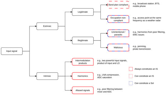
Notably, the IS does not always come from a signal transmitted voluntarily or involuntarily (a signal source extrinsic to the receiver). Situations arise in which the IS degrading the monitoring performance originates from inside the receiver itself (a signal source intrinsic to the receiver). Extrinsic IS can be a legitimate signal emitted according to the local band-plan, at a legal power limit, with adequate filtering (such as a broadcast radio station, a mobile network base transceiver station (BTS), …). These can also be parasitic and unintentional signals (such as harmonics generated by an emitter with improper filtering, defective devices generating out-of-band transmissions) or stem from illegitimate or malicious sources (jamming, pirate transmissions, …). Figure 1 represents a non-exhaustive list of possible signals found in the RF spectrum.
Figure 1.
Classification of signal sources reaching the receiver by origin and legitimacy. An extrinsic signal can be an IS, SoI or uninteresting depending on the situation. A non-compliant or illegitimate signal usually is either an SoI or IS. An intrinsic signal is always considered an IS.
Intrinsic IS can be intermodulation products, harmonics, or aliased signals, most often stemming from the memory effects of the analog front-end (AFE) [1]. Those intermodulation products or harmonics can be caused by extrinsic IS which are outside the part of the spectrum being monitored. As such, the counter-measures to put in place to reduce the impact of intrinsic IS need to operate over a larger bandwidth than that of the receiver.
In the same way, the SoI can also be a legitimate signal transmitting within the local band-plan (such as a mobile phone or other low-power transmitters) or a legitimate signal not following the channel access and occupation rules (such as an improperly configured access point transmitting at the same frequency as a radar) or an illegitimate signal (such as observed earlier).
Legitimate signals follow the regulatory band-plan but because the parasitic and unlawful signals do not, no assumption can be made about the frequency, content, and modulation types of SoI or IS. As such, no pre-built, fixed filters can be used to filter out extrinsic ISs. Any solution based on traditional methods such as automatic gain control, or in-line attenuators would not be adequate as these would simply attenuate all signals (IS or SoI) indifferently and as such do not impact the dynamic range. Because the frequency of the SoI and IS are not known, techniques that involve frequency slicing such as channelized receivers and filter banks are not considered either as they do not address the source of the problem.
Relying on this context, this paper first explains the source of the limited dynamic range in SDR receivers, as well as the main figures of merit regarding dynamic range and their meaning. It then evaluates what room for improvement remains in the components forming the receiver. Next, potential solutions to reduce the dynamic range of the received signal are explored starting with beamforming techniques and then frequency filtering techniques. Essential digital techniques are also covered before concluding.
2. Dynamic Range
In most wideband SDR receivers, the global dynamic range is limited by the dynamic range of the analog-to-digital converter (ADC). Examples are the LMS7002m from Lime Microsystems with a specified dynamic range of 60 dB [2] or the BladeRF 2.0 series (using an AD9361) which also has a dynamic range of around 60 dB. This value was experimentally measured on a BladeRF 2.0 xA4 at 433.5 MHz, with the front-end gain set at midpoint and the fastest sampling rate of 61.44 Msps. These values are given as examples and show that the order of magnitude for a commercial SDR’s dynamic range is around 60 dB. The precise value is of secondary importance because any careful system designer should account for a sufficiently large margin of error. The ADC constrains the dynamic range of the system by limiting both how strong a signal can be before clipping and how weak a signal can be before its signal-to-noise ratio (SNR) becomes too low. When considering the full bandwidth of the converter (BWADC), the theoretical maximum dynamic range (DR), expressed in dB, is given by Equation (1)
with being the resolution of the converter in bits. However, this theoretical maximum is, in practice, limited by distortions within the converter such as harmonics or intermodulation products. When accounting for the noise and the non-idealities of the components causing signal degradation, the signal-to-noise and distortion ratio (SINAD) is considered and can be expressed as an effective number of bits (ENOB) according to Equation (2)
The ENOB expresses the exploitable resolution of the converter when assuming a uniform distribution of the noise power and is lower than the converter resolution. In addition, the imperfect conversion along with noise from the surrounding circuitry causes spurious signals, which manifest as narrow-band low-power signals appearing in the digitized version of the signal. The power of the various spurious signals is generally below the total power of the noise and distortions, but because these spurious signals are narrower in bandwidth than the quantization noise, they have a higher local noise density than the quantization noise, and a characteristic bandwidth (BWc) has to be considered. This characteristic bandwidth can be the width of a fast Fourier transform (FFT) bin when computing the spectrum of the signal, often the case when performing dynamic range measurements or spectrum monitoring, or the bandwidth of a band-pass filter based on the width of the SoI. When taking this characteristic bandwidth into account, and assuming a uniform distribution of the quantization noise, the actual dynamic range is increased according to Equation (3)
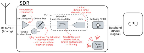
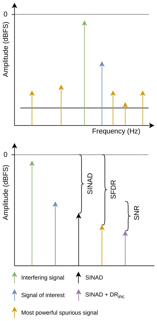
The spurious signals, if they are comparable in bandwidth to or smaller than BWc, keep the same power level, usually staying above the noise floor. The dynamic range computed between the maximum input power and the strongest spurious signal is called the spurious free dynamic range (SFDR). When performing spectrum monitoring tasks, because no assumption can be made about the frequency of either the SoI or the IS, one must assume that they will overlap, hence forcing consideration of the SFDR. When taking the AFE into account, additional intrinsic ISs are generated by the various components of the receiver (see Figure 2 for a representation of intrinsic IS sources within an SDR receiver using intermediate frequency (IF) sampling), further reducing the SFDR.
Figure 2.
Various sources of intrinsic ISs in a typical SDR receiver using IF sampling.
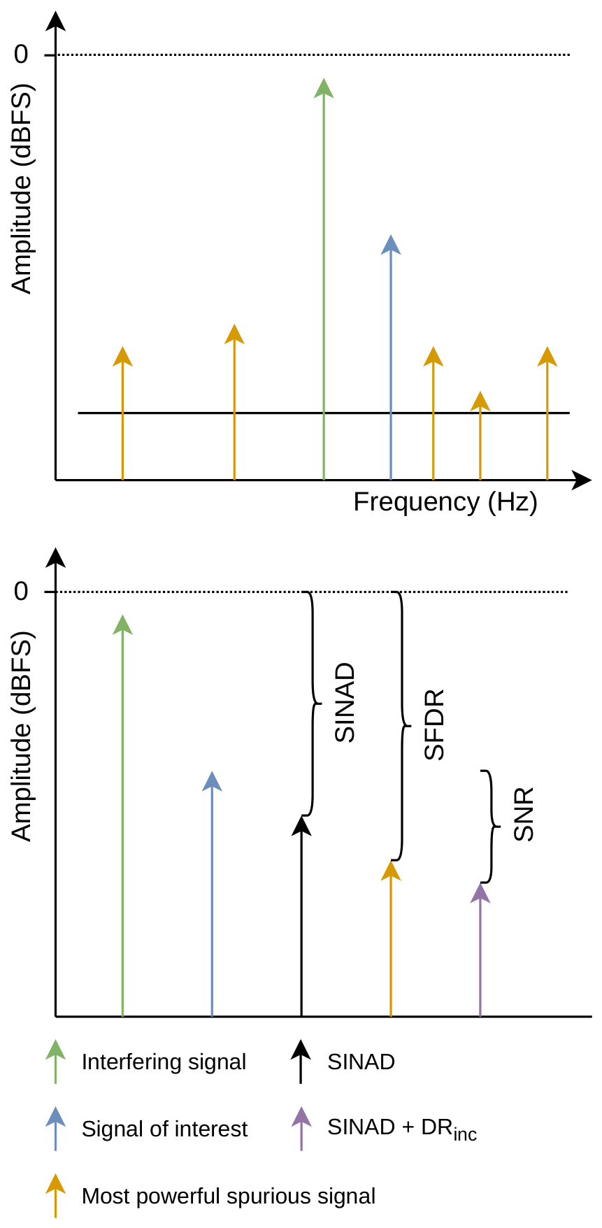
In Figure 3, a hypothetical scenario illustrates the spectrum at the output of an ADC. The top image shows a spectral view of the IS and SoI along with several spurious signals as seen by the ADC. The gain of the AFE is selected so that the most powerful signal stays a few decibels below the full scale of the ADC. The noise floor of the ADC is usually well above the thermal noise floor of the AFE, and the SoI is surrounded by various spurious signals. The bottom image shows a comparison between the IS, SoI, ADC dynamic range, SFDR, SINAD, SNR and the worst-case SNR (using the full bandwidth of the receiver without any post-acquisition filtering).
Figure 3.
(Top): Representative spectrum of the digital signal after the ADC. (Bottom): Graphical representation of the SINAD, SFDR and SNR.
As an example, consider an SoI with a bandwidth of 12.5 kHz and requiring 10 dB of SNR for proper reception. The receiver has a 3.2 GHz bandwidth. Applying this scenario to Equation (3) shows that the dynamic range is increased by 54 dB compared to the SINAD computed from the ENOB alone, but the signal itself needs to be maintained 10 dB above the noise floor. This improved dynamic range does not take spurious signals into account, which are strongly related to the specific component used and its integration in the receiver.
3. Comparison Criterion
The next four sections explore and compare various techniques that help improve the dynamic range of a spectrum monitor. Each section and each technique bring improvements along several axes which are compared in Section 8. The comparison is done along the following criteria:
- Attenuation of extrinsic ISs is the difference in amplitude between the most powerful and least powerful signals reaching the ADC.
- Improvement in dynamic range after the ADC is the difference in amplitude between the most powerful and least powerful signals in the digital domain, accounting for intrinsic ISs introduced by the AFE and the ADC.
- UAV suitability is given mainly by the size, weight and power (SWaP) of the technique. The major criteria are the size and weight of the implementation. The power consumption is usually small compared to the power consumption of the aircraft itself; however, a design drawing too much power may need adequate heat dissipation, hindering UAV suitability. Another criterion evaluated is the computing power required as a large computing power can be difficult to accommodate aboard an aircraft.
- Hardware complexity is the estimated difficulty in implementing the hardware aspects of the technique.
- Software complexity is the estimated difficulty in implementing the software aspects of the technique.
- Instantaneous bandwidth is the maximum bandwidth of the signal that the technique can attenuate at a given time.
- Tuning bandwidth is the difference between the highest and lowest center frequencies of the signal that the technique can attenuate at different times.
4. Component-Centered Improvements
4.1. Analog Front-End
The first step to limit the various ISs is to avoid the appearance of intrinsic ISs in the AFE of the receiver. As such one must observe three principles: simplifying the AFE as much as possible by reducing the number of active components, choosing them as linear as possible, and using adequate gain or attenuation control to avoid saturation. Regarding the simplicity of the front-end, the best situation is achieved with direct-sampling receivers where the signal from the antenna goes directly to the ADC after passing through an optional low-noise amplifier (LNA). In designs not using direct sampling, a mixer must be introduced between the antenna and the ADC along with image rejection and IF filters, which can introduce extra nonlinearities. In both direct and IF sampling, anti-aliasing filters must be used if the ADC risks sampling signals over more than a single Nyquist zone.
The linearity of an LNA can easily be assessed. Commercial devices exist with a high linearity over a wide bandwidth and a compression point well above the full-scale amplitude of high-speed ADCs [3,4,5]. With such devices, the ADC saturates before the LNA enters the compression region, avoiding the creation of distortions through intermodulation. Mixers are, however, inherently nonlinear devices and can output signals outside the first Nyquist zone of the ADC. Additionally, if the noise figure of the front-end is low enough, the noise added by the front-end is negligible compared to the quantization noise of the ADC. Moreover, the more linear analog components are, the higher their power consumption tends to be. This can prove challenging in embedded systems with limited available power or heat-dissipation capacity.
In summary, all these criteria need to be traded off in order to reduce the appearance of signal distortions during spectrum monitoring while keeping the receiver compact and low power.
4.2. Analog-to-Digital Converter
The dynamic range of an ADC is not only limited by the quantization noise, noise figure, and distortions but also by the other spurious artifacts added by the converter itself during conversions.
In order to improve the overall dynamic range of the receiver by improving the dynamic range of the ADC, the main figure of merit to consider is the SFDR. There is, however, a trade-off between the dynamic range and the sampling speed of an ADC. A direct-sampling spectrum monitor requires a sampling rate of at least 6 Gsps in order to monitor signals from 0 GHz to 3 GHz. This allows it to cover the whole band continuously, increasing the probability of intercepting the SoI. At these sampling rates and resolutions, state-of-the-art converters are designed by time-interleaving several successive approximation ADC slices [6,7,8,9,10]. This causes additional challenges as the slices must be perfectly matched and aligned in order to avoid creating distortions and spurious signals [11]. The main effect of timing errors between ADC slices is an increase in the amplitude of spurious signals. These are more difficult to attenuate as the frequency of the input signal gets closer to the sampling bandwidth [12]. With proper calibration techniques, the degradation of SINAD caused by time-interleaving can be contained to below 2 dB. If the input signal frequency does not get too close to the sampling bandwidth, the SFDR of an ADC using time-interleaving can be kept to about the same as the SFDR of individual slices [9,13,14,15,16,17].
From [6,7,8,9,10], the state-of-the-art SFDR when considering signal bandwidths nearing the sampling bandwidth ranges between 60 dB and 70 dB. Increasing the sampling bandwidth of the ADC above the monitored bandwidth helps keep the SFDR as high as possible.
The commercially available ADC [5] detailed in [18] exemplifies the capabilities attainable by commercially available components. When in interleaving mode, it has a 3.2 GHz bandwidth with an SFDR of 70 dB (for small signals, measured 12 dB below full scale) and an ENOB around 8.5, translating to a SINAD of 53 dB. This measurement requires the most powerful signal to be substantially below full scale, which reduces the usable dynamic range further. The power consumption of this ADC is 6.6 W, but this does not account for the power consumption of the Field-Programmable Gate Array (FPGA)-based system that must process the data, including performing the timing calibration of the ADC slices.
The commercially available AFE LMS7002M from Lime Microsystems has an SFDR of 60 dB and an ENOB of nine, translating to a SINAD of 56 dB [2].
Reconsidering the example of a 12.5 kHz SoI requiring an SNR of 10 dB, we can consider two situations. In a first situation, the SoI is known to be far enough from any spurious signal. If the SoI is digitized by the ADC from [5], one can use Equation (3) to obtain Equation (4), which gives the minimum acceptable power level below full-scale for the SoI in ideal conditions.
In the same situation, if the SoI is now digitized by the LMS7002M at its widest bandwidth (61.44 Msps), one gets Equation (5), which gives the minimum acceptable power level below full-scale for the SoI in ideal conditions.
This situation is quite advantageous for both ADCs. However, if the exact frequency of the SoI is not known, then the possibility that it will overlap with a spurious signal must be considered. In this new situation, if the SoI is digitized by the ADC from [5], Equation (3) now gives Equation (6), which gives a significantly higher minimum acceptable power level below full-scale for the same SoI.
In that same new situation, if the SoI is now digitized by the LMS7002M at 61.44 Msps, Equation (3) gives Equation (7) for the minimum acceptable power level below full-scale:
These numbers might be even lower in the presence of additional extrinsic or intrinsic ISs. A strong IS would set the power corresponding to the full scale, potentially bringing the SoI too low relative to the noise floor for proper reception.
Putting in place even the most advanced counter-measures do not satisfactorily improve the performance of a system with an inadequate hardware design. The selection of a proper ADC is foundational in ensuring the highest possible performance of a spectrum monitoring system but is not sufficient in high-dynamic-range environments.
5. Beamforming-Based Techniques
Beamforming consists of using an array of antennas to alter the radiation pattern of the receiver, usually creating local maxima to increase the gain of the receiver in a specific direction. This beam can then be steered in a chosen direction to favor signals coming from that direction. Beamnulling is a similar technique except that the beam creates local minima to attenuate the signal from specific directions. In use cases where it is desirable to attenuate a powerful signal, beamnulling techniques are more appropriate as the origin direction of the SoI is not yet known, whereas the IS, being strong, is easier to identify and locate. In this section, the term beamforming is used to refer to both beamforming and beamnulling as the hardware implementations are mainly the same. One major difference to consider is that the maximum gain of a beam in a beamformer system follows a relationship described by (8).
where G is the gain of the beam, and is the number of antennas in the array. This implies that large gains require a large number of antennas. Beamnulling systems can theoretically provide perfect attenuation and in practice can easily achieve several dozen dB of attenuation with a reduced number of antennas [19]. The number of antennas impacts the width of the nulls created as well as their number. An antenna array of size is able to generate at most nulls [20].
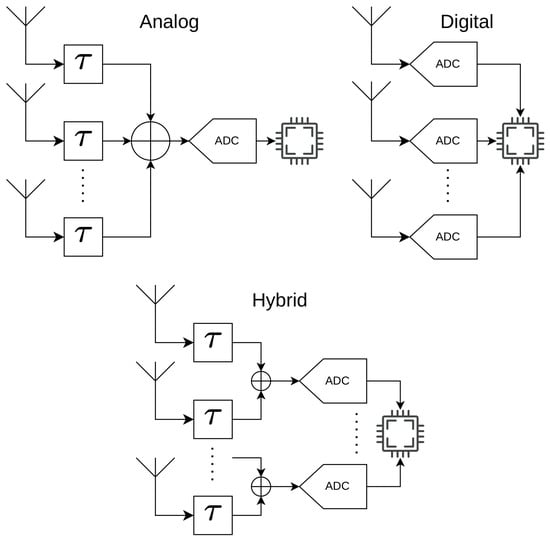
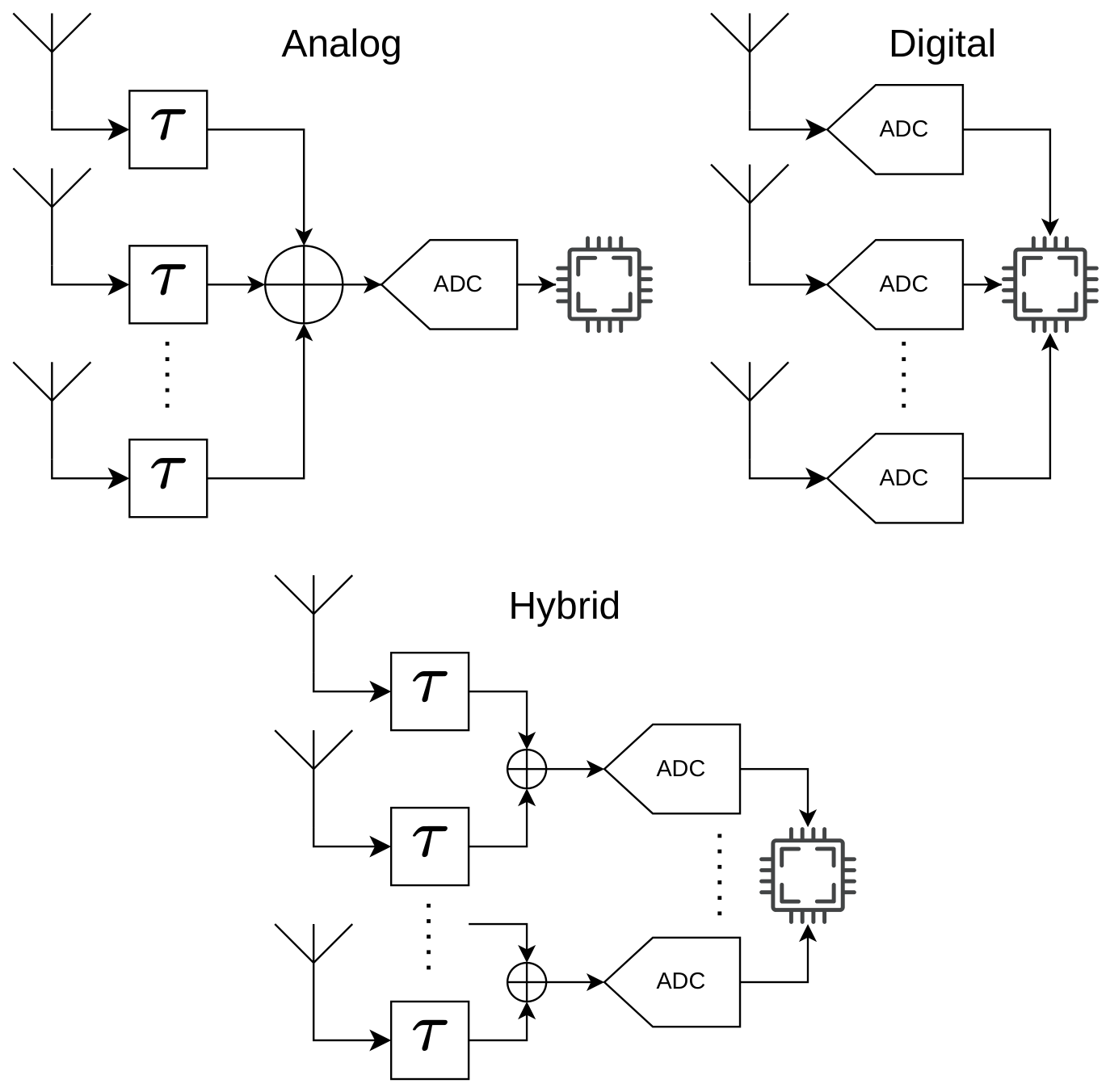
The beam is steered and shaped by time-shifting and modifying the amplitude of each input signal from each antenna. For a receiver composed of two antennas that must be able to steer a beam across 360°, the maximum delay to be applied to the signal is equal to the propagation delay between the two antennas. Depending on whether the operations are performed in the analog or digital domain, beamforming can be classified into two groups: analog beamforming and digital beamforming. A third category exists, hybrid beamforming, using stages of both analog and digital beamforming to exploit the advantages of both systems. Figure 4 gives an overview of the three categories of beamforming.
Figure 4.
The three families of beamforming methods. LNA and other AFE components such as mixers are not represented here.
The main downside of beamforming is that it requires an array of antennas, increasing the spatial footprint of the receiver. Furthermore, the antennas’ size and spacing are proportional to the largest wavelength the receiver must be able to receive. Reduced spacing induces coupling between the antennas, leading to poor performance while increased spacing increases the footprint of the array with diminishing returns in beam quality.
Having antennas too close to one another leads to coupling between the channels which reduces the gain of the beam or the attenuation of the nulls. It is generally considered that to minimize coupling effects, a minimum distance of must be respected between antennas, with being the wavelength corresponding to the lower bound of the receiver’s bandwidth. Larger distances lead to less coupling. Under that condition, a system with three antennas, operating at a frequency as low as 100 MHz, requires a minimum bounding triangle of 1 m2. A similar system using four antennas requires a minimum bounding rectangle of 2.2 m2. The size of those two surfaces is reduced to 0.11 m2 and 0.25 m2 respectively when operating at 300 MHz.
Beamforming is able to attenuate extrinsic ISs, thus reducing intrinsic ISs if those happen to originate from the high power of an extrinsic IS. Beamforming techniques do not apply if the IS and SoI come from the same direction.
Two main use cases for beamforming are considered. Many modern communication systems use beamforming techniques as a way to increase the user density, i.e., forming multiple beams at the same frequency to multiply the number of data streams or as a way to counteract strong free-space path loss (FSPL) in the band of operation [21,22,23]. In this use case, however, the dynamic range of the receiver is not the primary motivation for using beamforming; it is the need to spatially distinguish the various data streams coming from different directions at the same frequency. A second use case for beamforming is the ability to amplify or attenuate signals from a specific direction whenever the SoI is too weak to be received using an omnidirectional receiver [24,25] or when the systems operate over several frequency bands with a varying FSPL.
In wideband receivers, two harmful effects can be observed. The first is called beamsquint and arises when the effective beam angle varies with the frequency. The second is called angular ambiguity and can be observed at frequencies whose wavelength is more than twice the antenna spacing. In the case of beamnulling for example, beamsquint can cause the null in the radiation pattern to move in an undesirable direction, potentially attenuating the SoI that the system should have detected, in addition to not attenuating the IS that is degrading the dynamic range. Angular ambiguity can cause additional beams or nulls (side lobes) to appear at higher frequencies, and attenuate other signals than the IS, again potentially preventing the detection of the SoI. These effects are very limited in narrow-band communication systems.
5.1. Analog Beamforming
In analog beamforming techniques, the signals coming from the antennas are shifted and summed before the digitization stage (ADC). This has the advantage that, particularly in the case of beamnulling, it can reduce the dynamic range of the signal to digitize, relaxing the requirements on the ADC. Linearity requirements of the AFE still apply, and the components located before and up to the final adder must still be sufficiently linear so as to avoid creating intrinsic ISs. Forming the beam is done by phase-aligning the signal coming from the target direction and received through the antennas of the array. The alignment can be realized using two main techniques.
The first technique involves applying a frequency-independent phase-shift to the signals from the antennas. This phase shift is determined by the target angle of the beam or null, the spacing between the antennas in the array and the operating frequency. It is the most straightforward technique to implement but because the required phase shift is inherently related to the operating frequency, the angle of the beam varies across the receiver bandwidth, creating significant beamsquint.
The second technique uses true time delay (TTD) to apply an actual (true) time delay to the signal. This time delay translates to different phase shifts at different frequencies, theoretically preventing beamsquint. This makes TTD much more suitable for wideband systems such as spectrum monitoring systems. In practice, however, the actual delay varies with respect to frequency and this also induces beamsquint although much less than when applying constant phase shifts [26].
TTD can be applied at various places along the path of the signal [27]. The most obvious place is along the transmission line connecting each antenna to the adder. The delay induced by that transmission line can be modified by either changing the propagation delay or the length of the transmission line (for example, using switched transmission lines) [28]. Variations of these approaches exist such as the Rotman lens where pre-set beam directions are formed through a specific physical feature performing the delay and summation at the same time. The size of those physical features is proportional to the wavelength at which the lens must operate, making this method impractical for use at lower frequencies.
The signal can also be delayed by placing an adder between the sample and hold (S/H) cells and the ADC input. The S/H cells can then be driven with time-shifted clocks, delaying the signal. The downside of this method is that it limits the maximum delay applicable to the signal to one sampling clock delay per successive S/H. The maximum distance between the antennas in the array or maximum target angle of the beam are thus limited, especially in systems with large bandwidth such as high-speed direct-sampling receivers [19].
Analog beamforming, by being in the path of the analog signal, introduces insertion losses potentially impacting the gain requirements of the AFE or the received signal strength of the SoI. These insertion losses can also vary with the frequency, influencing the shape of the beam, the gain or attenuation provided. Analog beamforming can also increase the risk of generating intermodulation products before the digitization stage if additional nonlinear components are in the signal path.
The design in [19] reported reaching an attenuation of 20 dB with 100% bandwidth at a center frequency of 2 GHz using an analog beamformer.
5.2. Digital Beamforming
In digital beamforming techniques, each antenna of the array is connected to one ADC (or ADC channel). The beam is then formed using digital signal processing (DSP) techniques in the processor after the signal is digitized. The immediate effect of this is that each channel still has to digitize the complete spectrum including the IS and SoI whose power has not been altered. As such, the beamforming itself does not improve the dynamic range of the receiver.
The multiplication of digital data streams requires heavy computing capabilities and increases the energy consumption [29], this effect being even more prominent at high sampling rates as is the case in wideband receivers. However, this simplifies the front-end, reducing the number of components required between the antenna and the ADC.
Only a slight dynamic range improvement might come from the averaging effect of the noise coming from the various ADCs (assuming the noise between the channels is uncorrelated). This effect improves the SNR according to (9)
with being the number of digital channels. Because IS are not random uncorrelated noise, they are not attenuated by this averaging effect.
This technique is usually implemented when the receiver receives several signals at the same or similar frequencies, from different directions and with power levels within the ADC capabilities. In that case, digital beamforming is able to discriminate between the various signals. This technique is thus suitable if the IS is at the same frequency as the SoI and of comparable amplitude, causing the SNR of the SoI to be too low for proper exploitation of the signal. Finally, because the beamforming operations are performed in the digital domain, the data streams can be duplicated in order to create multiple independent beamformers, but each beamformer is only able to have at most one less beam than the number of antennas.
5.3. Hybrid Beamforming
In hybrid beamforming, concepts from both analog and digital beamforming are used. Antennas in the array are grouped into sub-arrays using analog beamforming, the outputs of which are then combined using digital beamforming. The digital beamforming step enables more fine-grained delay between streams than analog TTD. It also enables the exploitation of spatial diversity from the antenna array [30] and more complex analysis such as direction finding of the various SoI or IS. The analog beamforming part has the role of reducing the dynamic range of the input signal before it reaches the ADC. Hybrid beamforming has the disadvantage of having fewer nulls to steer and requiring more ADC channels.
5.4. Summary
Beamforming is a versatile technique that can either amplify or attenuate signals from specific directions. Its implementation must be carefully chosen as only analog beamforming can efficiently reduce the dynamic range of input signals and more specifically, only true-time delay allows sufficient reduction in beamsquint. Though beyond the scope of this paper, and unlike simple component upgrades, beamformers require a control system whose role is crucial in ensuring attenuation of the proper signals.
6. Frequency Filtering
Frequency filtering is an obvious candidate for interference rejection in spectrum monitoring receivers through the use of band-stop filters (BSFs). Unlike beamforming systems, they require only one antenna to operate, reducing the footprint of the system. The goal is to reject the IS at specific frequencies with the obvious limitation that if the SoI and the IS are too close in frequency or overlap (such as in time-division multiple access (TDMA) systems or jamming) then the SoI will also be filtered out. This requires filters with both a variable center frequency and a variable bandwidth, which increases the receiver’s complexity.
Traditional frequency filtering is implemented with discrete passive components and assembled in filter banks, but because of the frequency flexibility requirements for spectrum monitoring, this is not a viable alternative as this would produce bulky systems. Implementations with discrete passive variable components do not show enough flexibility to be suitable either [31]. Filters with such requirements in terms of flexibility are called hyperflexible RF filters or frequency-agile RF filters.
Many types of implementations exist but almost all have the common limitation that the number of signals that may be simultaneously filtered out is implementation-dependent.
One major family of BSFs uses multiresonant cells, or frequency-tunable resonators. The tunability of the system can be a limiting factor as these implementations have a center frequency that varies in the 1 GHz to 2 GHz range [31]. One implementation in particular has a notch depth of −17 dB to −46 dB in the 1.8 GHz to 2.16 GHz frequency range [32]. Other tuning implementations using liquid metal or liquid crystal manage to go beyond that tuning range, but their size limits them to higher frequencies (typically above 3 GHz) [33,34]. Their filtering capability is usually suitable for narrow-band ISs with the possibility of arranging several transmission zeroes in close proximity to trade attenuation for bandwidth.
N-Path filters work by frequency-shifting the input signal then applying a filter with a known frequency response. This has the benefit of being widely tunable by shifting the frequency flexibility burden away from the filter implementation [35]. Most of those implementations, however, focus on implementing band-pass filters (BPFs), which are suitable when the frequency of the SoI is known. They provide wider filtering capability than multiresonant cells, with a bandwidth of up to 80 MHz. The design in [35], while implementing a band-pass and not a band-stop filter, reaches a >24 dB rejection of out-of-band signals with a bandwidth of 5 MHz to 80 MHz and a tuning frequency of 1 GHz to 5 GHz.
Both multiresonant-cells and N-path filters are directly in the path of the analog signal and need to present a low insertion loss in order to avoid attenuating the SoI.
Feed-forward decoupling is a technique that digitizes the IS and process it using DSP to synthesize a mirror image of the signals to decouple them from the main analog path using a feed-forward loop [36]. The addition of a digital processor in the path of the strongest signal opens the possibility for advanced processing including very sharp frequency responses or multiple notches in close proximity. The limitations are the digital delay added by the DSP filtering operations and the bandwidth of the digital system. This specific layout helps reduce the insertion losses and makes it possible to bypass the filter which is not as easy if the filter is directly in the path of the digitized signal. The implementation from Ref. [36] obtains an attenuation of ISs of 24 dB to 32 dB with a bandwidth of 1 MHz to 8 MHz per signal attenuated. The center frequency ranges from 800 MHz to 1800 MHz and attenuates eight signals simultaneously within 200 MHz.
Frequency filtering is a complementary solution to beamforming in that it allows one to cover different use cases such as signals coming from an identical direction. There are many existing implementations but few offer the wide bandwidth required by spectrum monitoring receivers, with N-path filters being a prime candidate for implementation.
7. Digital Processing Techniques
A range of techniques that mostly require digital processing exists to lessen the impact or the creation of spurious signals.
Non-uniform sampling, also called compressive sensing, allows one to extend the bandwidth of a receiver beyond a single Nyquist zone by sampling the signal at irregular intervals, reducing aliasing. This requires fine control over the sampling clock of the ADC, or several ADCs driven at varying sampling rates. This does not attenuate ISs and requires additional computing power to improve the digitized bandwidth over what the monitoring system requires [37,38].
A nonlinear equalizer (NLEQ) is a technique that uses digital signal processing to reduce the amplitude of various intrinsic ISs originating from nonlinearities in a signal path. In a receiver, this is done post-acquisition by processing the received samples using a model of the front-end. This model is usually based on Volterra series to take the memory effect of semiconductors into account [39]. Applying an NLEQ to an input signal typically requires several hundred operations per sample, preventing real-time operation in wideband receivers. According to [40], the power of intermodulation products created within the ADC can be reduced by 16 dB with a cost of 110 operations per sample. This translates to an improvement of the SFDR of the receiver by at most 16 dB on the condition that the limiting factor in SFDR is the spurious signals created by the ADC. As such, it does not improve the SINAD of the receiver, only the SFDR.
Modulo-sampling is a technique that applies a modulo operator to the signal before sampling in order to prevent the ADC from saturating. This requires dedicated circuitry for the modulo operation. This circuit does not yet reach the sampling rate required for RF signals and spectrum monitoring but can enable a large increase in the ADC’s SINAD. Modulo-sampling requires computationally heavy reconstruction algorithms [41,42,43], making this perspective difficult to integrate into airborne wideband receivers.
8. Discussion
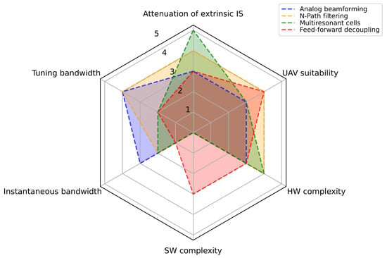
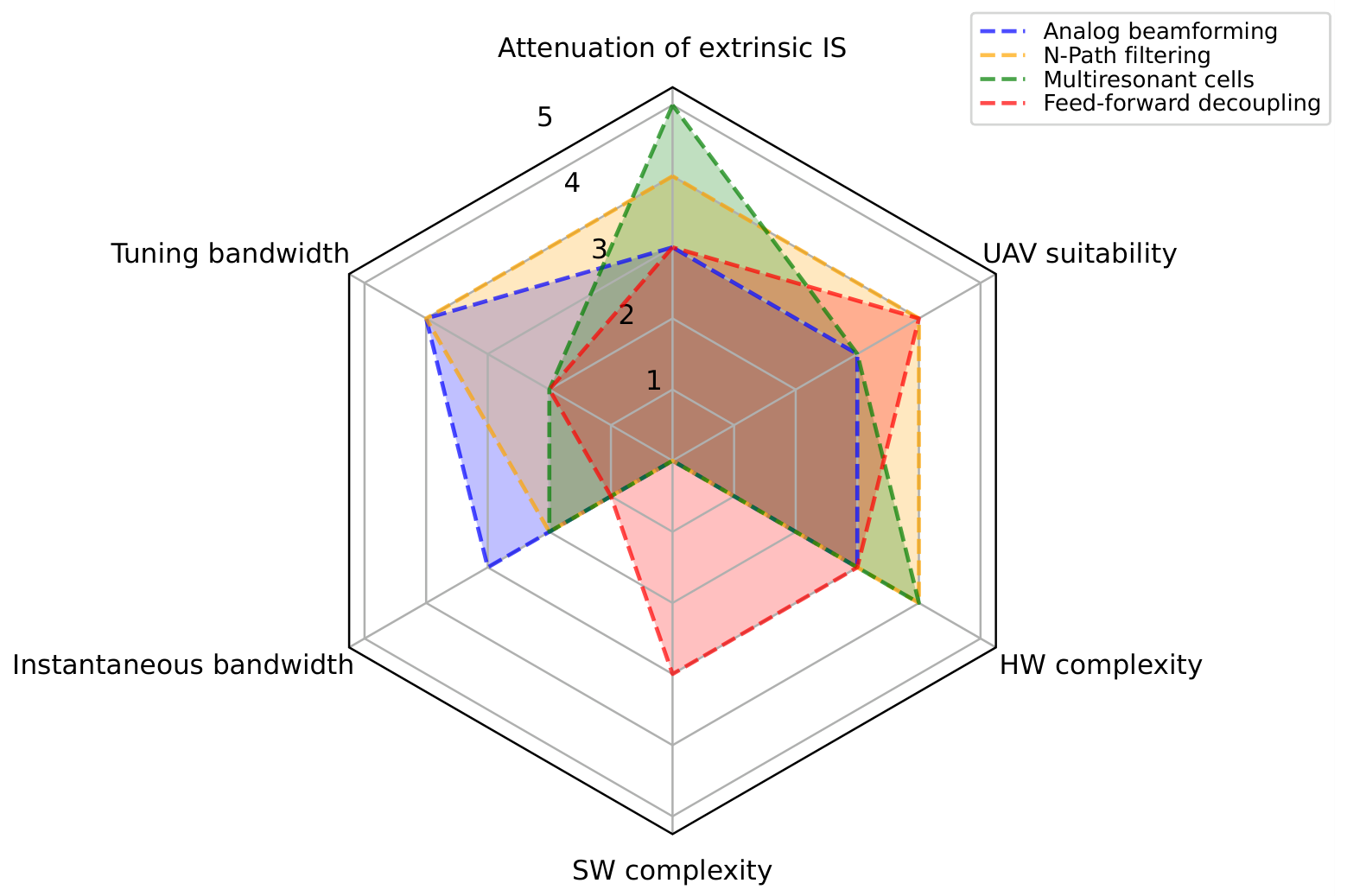
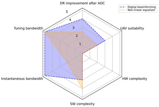
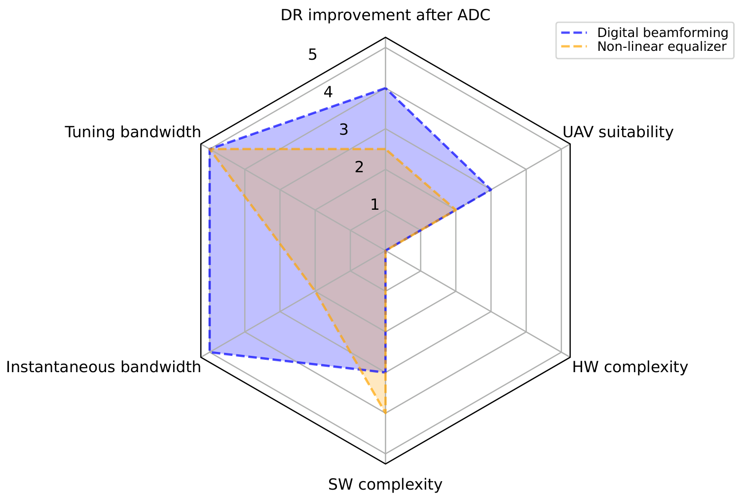
As can be seen in Figure 5, only some techniques among the several explored in this paper can block ISs in a way that reduces the dynamic range of the input signal before the ADC. Other techniques, compared in Figure 6, provide post-processing dynamic range improvement after the ADC (digital beamforming, nonlinear equalizers). Hybrid beamforming are not represented as it can be considered a composite of both analog and digital beamforming. Compressive sensing does not significantly improve the dynamic range in any way, and the maximum sampling frequency of modulo sampling does not match the requirements for use in spectrum monitoring systems. As such, these techniques are not discussed.
Figure 5.
Comparison of the techniques improving the dynamic range before the ADC along the attenuation of extrinsic ISs, the suitability to unmanned aerial vehicles, the hardware and software complexity, the instantaneous bandwidth and the tuning bandwidth.
Figure 6.
Comparison of the techniques improving the dynamic range after the ADC. Comparison along the improvement in dynamic range, the suitability to unmanned aerial vehicles, the hardware and software complexity, the instantaneous bandwidth and the tuning bandwidth.
The techniques discussed in this paper are briefly summarized below according to the criteria exposed in Section 3.
Analog beamforming provides excellent tuning bandwidth with a very wide instantaneous bandwidth if implemented using TTD, the limiting factor being beamsquint. The expected IS attenuation before the ADC is around 20 dB. The UAV suitability of all types of beamforming is hindered by the footprint of the antenna array, limiting the beamforming techniques to only the largest UAVs, especially at lower frequencies. The complexity of analog beamforming comes mostly from the hardware implementation, with hybrid beamforming in particular inheriting the hardware complexity of analog beamforming and the software complexity of digital beamforming.
N-Path filtering has a good tuning bandwidth because the switches are responsible for tuning the center frequency while the instantaneous bandwidth is more limited, reflecting the difficulty of implementing filters with a highly flexible bandwidth. N-Path filters have a particularly good IS attenuation before the ADC reaching up to 50 dB. The UAV suitability is also good as the system has no moving parts, a limited physical footprint, low power consumption and low-computing-power requirement. The complexity of implementation is hardware.
Multiresonant cells have a poor, implementation-dependent tuning bandwidth and no single method can cover a significant portion of the frequencies below 3 GHz. The instantaneous bandwidth of multiresonant cells has the same limitation as N-Path filters. They do provide the best IS attenuation before the ADC, reaching up to 70 dB. Their UAV suitability is limited by the need to assemble the filters in banks, increasing the size and weight of the implementation and yielding particularly high hardware complexity. Moving parts and liquid materials make some implementations sensitive to vibrations, further reducing UAV suitability.
Feed-forward decoupling presents a limited instantaneous bandwidth due to the DSP in the feed-forward loop. The tuning bandwidth is also limited by the coupling and decoupling stages in the signal path. The expected IS attenuation before the ADC is around 20 dB. UAV suitability is quite good, with the main limiting factor being the required computing power that is proportional to the instantaneous bandwidth. This technique involves both hardware complexity for the proper coupling and decoupling stages and software complexity for the implementation of adequate high-speed DSP.
Digital beamforming has an excellent tuning bandwidth, equal to the instantaneous bandwidth. The attenuation of IS post-ADC can reach 20 dB but this neither prevents nor attenuates the spurious signals created in the AFE due to excessive signal strength. The dynamic range improvement in hybrid beamforming attributable to the digital beamforming part is limited but both tuning and instantaneous bandwidth benefit from the digital beamforming part. Both digital and hybrid beamforming (like analog beamforming) have a reduced UAV suitability due to the footprint of the antenna array. Digital beamforming does have low hardware complexity.
The instantaneous bandwidth of NLEQ is limited to the number of operations per second the DSP is capable of. NLEQs do not limit the tuning bandwidth of a system. The SFDR improvement after the ADC is slightly below 20 dB, but, contrary to digital beamforming, it does reduce the spurious signals created in the ADC by powerful extrinsic ISs. This improvement can be complementary to the improvements in dynamic range obtained before the ADC through other techniques. The UAV suitability is also limited by the computing power aboard the vehicle. The implementation complexity of an NLEQ is only due to software, requiring a good digital model of the AFE and suitable computing power.
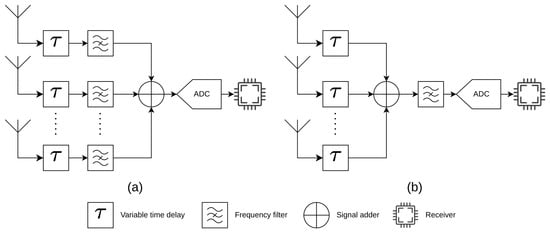
The techniques discussed can be combined to cover a more comprehensive range of use cases, such as spatial and frequency overlap of the SoI and IS. Combining any form of frequency filtering or analog or hybrid beamforming with an NLEQ does not introduce any particular interaction. Combining frequency filtering with analog or hybrid beamforming, however, can be done in two ways. A frequency filter can be inserted in each branch of the beamformer, alongside the variable time delay. This multiplies the number of frequency filters and requires that the frequency filters in each branch be very similar at the risk of degrading the beamformer performance. If this is undesirable, a frequency filter can be added after the adder of the beamformer. This reduces the number of frequency filters to one per ADC channel, but increases the risk of having an IS creating distortion in the adder of the beamformer. Figure 7 exemplifies the two proposed architectures. Combining analog or hybrid beamforming with feed-forward decoupling could benefit from merging the variable time delay of the beamformer with the time delay of the feed-forward decoupler for a reduced layout footprint. This, however, adds a dependency between the variable delay setting of the beamformer and the digital processing of the feed-forward decoupler.
Figure 7.
Two architectures combining spatial and frequency filtering. In (a), frequency filters are placed alongside each variable time delay of the beamformer. In (b), the frequency filter is placed after the adder.
As an example of what such a system could provide, consider the previously mentioned 6.4 Gsps ADC with a SINAD of 53 dB and an SFDR of 70 dB. It receives two signals. The IS is a 4 kW broadcast signal from a known location 5 km away at 442 MHz. The SoI is a concealed global navigation satellite system (GNSS) jammer in a vehicle outputting a 0.1 W tone at 1572 MHz. The signal is attenuated by 14 dB exiting the vehicle. In order to prevent intrinsic ISs from being created in the ADC, the AFE gain is set such that the IS is 12 dB below full-scale.
When observing the spectrum through a 1024-point FFT, Equation (3) gives a noise floor of 83 dB below full scale. Under these conditions, the SoI is received 10 dB above the noise floor at a distance less than 450 m. If a beamnulling system were able to attenuate the IS by 20 dB, the same SoI could be sensed from a distance of 4.5 km. In the meantime, a frequency filter could filter out signals in the 2400 MHz band that may emanate from other moving vehicles close to the SoI. If the limiting factor is the SFDR, the SoI would be received 10 dB above any spurious signal at a distance less than 100 m. A beamnulling system with an attenuation of 20 dB would allow the same signal to be received from a distance of 1 km. An NLEQ could be added to the ADC digital processing system, lowering the SFDR by 16 dB and bringing it to a level comparable to the SINAD with a computing load of around 682 × 109 operations per second.
Note that this is a simplified example that assumes free-space propagation losses and that the frequency of the SoI is known. Those are not always observed, and in practice, the propagation losses for a close-to-ground vehicle would be much higher than those from a high-altitude broadcast antenna. Furthermore, the signal processing capabilities needed to detect and locate the SoI are not discussed.
9. Conclusions
While the wide bandwidth and advanced capabilities of software-defined radio (SDR) receivers make them well suited to spectrum monitoring, their performance is limited in terms of dynamic range. This work presented a comprehensive range of techniques along with the detailed limitations of each one.
A solution that uses hardware augmentations to attenuate ISs before the ADC is the most suitable. Such a system should combine several techniques like analog beamforming or N-path filtering and can also improve the SFDR after the ADC using, for example, an NLEQ.
Taking realistic use cases into account, there is also an advantage in being able to simultaneously perform spatial filtering (beamnulling) and frequency filtering (N-Path filtering, multiresonant cells or feed-forward decoupling) to cover a wider range of spectrum monitoring conditions. The development of such a platform, designed to filter signals in the frequencies from a few hundred MHz to 3 GHz, would significantly improve spectrum monitoring capabilities.
Author Contributions
Conceptualization, M.D.; investigation, M.D.; writing—original draft preparation, M.D.; writing—review and editing, M.D., J.P., S.A., J.-M.R.; supervision, J.P., S.A., J.-M.R.; project administration, J.P., J.-M.R.; funding acquisition, M.D., J.P., S.A., J.-M.R. All authors have read and agreed to the published version of the manuscript.
Funding
This work was funded by the Service Public de Wallonie Économie Emploi Recherche grant number 2410122.
Data Availability Statement
No new data were created or analyzed in this study. Data sharing is not applicable to this article.
Conflicts of Interest
The funding sponsors had no role in the writing of the manuscript; or in the decision to publish the results. Author Morgan Diepart is employed by SDR-Engineering. Author Jonathan Pisane owns stocks in company SDR-Engineering. Author Sylvain Azarian owns stocks in company SDR-Engineering. The remaining authors declare no conflicts of interest.
Abbreviations
The following abbreviations are used in this manuscript:
| ADC | Analog-to-digital converter |
| AFE | Analog front-end |
| BPF | Band-pass filter |
| BSF | Band-stop filter |
| BTS | Base transceiver station |
| DR | Dynamic Range |
| DSP | Digital signal processing |
| EMC | Electromagnetic compatibility |
| ENOB | Effective number of bits |
| FFT | Fast Fourier transform |
| FPGA | Field-Programmable Gate Array |
| FSPL | Free-space path loss |
| GNSS | Global navigation satellite system |
| IC | Integrated circuit |
| IF | Intermediate frequency |
| IS | Interfering signal |
| LNA | Low-noise amplifier |
| NLEQ | Nonlinear equalizer |
| SDR | Software-defined radio |
| SFDR | Spurious free dynamic range |
| S/H | Sample and hold |
| SINAD | Signal-to-noise and distortion ratio |
| SNR | Signal-to-noise ratio |
| SoI | Signal of interest |
| SWaP | Size, weight and power |
| TDMA | Time-division multiple access |
| TTD | True time delay |
| UAV | Unmanned aerial vehicle |
References
- Ito, H.; Fujii, T.; Yamao, Y. Post-Reception Compensation Performance of Blind Nonlinear Compensator with Equalizer against Memory Nonlinear Distortion. In Proceedings of the 2020 IEEE 92nd Vehicular Technology Conference (VTC2020-Fall); IEEE: New York, NY, USA, 2020; pp. 1–5. [Google Scholar] [CrossRef] [Scilit]
- LimeMicro:LMS7002M Datasheet—Myriad-RF Wiki. Available online: https://wiki.myriadrf.org/LimeMicro:LMS7002M_Datasheet (accessed on 20 August 2026).
- Mini-Circuits. CMA-103+ Ultra Linear Low Noise, Ceramic Monolithic Amplifier. Datasheet Rev. C. 2025. Available online: https://www.minicircuits.com/pdfs/CMA-103+.pdf (accessed on 12 September 2025).
- Macom. MAAM-011229 Broadband Low Noise Amplifier 0.05–4 GHz. Datasheet Rev. V3. 2025. Available online: https://cdn.macom.com/datasheets/MAAM-011229.pdf (accessed on 12 September 2025).
- Teledyne e2V Semiconductors. EV12AQ600/EV12AQ605 Quad 12-Bit 1.6 GSps ADC with Embedded Cross-Point Switch, Digitizing up to 6.4 GSps. Datasheet Rev. H. 2025. Available online: https://flir.netx.net/file/asset/68853/original/attachment (accessed on 12 September 2025).
- Shen, J.; Chen, W.H.; Burlinqame, E.; Weinreich, S.; Elliott, M.; McCracken, S.; Kenney, J.; Brunsilius, J.; Korkmaz, A.; Fontecilla, E.A.; et al. 24.8 A 12GS/s 9b 16× Time-Interleaved SAR ADC in 16 nm FinFET. In Proceedings of the 2025 IEEE International Solid-State Circuits Conference (ISSCC); IEEE: New York, NY, USA, 2025; Volume 68, pp. 442–444. [Google Scholar] [CrossRef] [Scilit]
- Hsieh, C.E.; Manganaro, G.; Liao, S.H.; Weng, J.; Fan, T.Y.; Chin, A.; Hung, T.C.; Wu, J.X.; Lo, C.L.; Pan, A.; et al. 24.6 A Power- and Area-Efficient 4nm Self-Calibrated 12b/16GS/s Hierarchical Time-Interleaving ADC. In Proceedings of the 2025 IEEE International Solid-State Circuits Conference (ISSCC); IEEE: New York, NY, USA, 2025; Volume 68, pp. 438–440. [Google Scholar] [CrossRef] [Scilit]
- Han, H.; Liu, S.; Liang, H.; Shen, Y.; Guo, J.; Ren, R.; Zhu, Z. A Power-Efficient Clock Circuit and Output Serializing Technique Integrated in a 12-Bit 10-GS/s ADC. IEEE Trans. Circuits Syst. I 2024, 71, 1495–1505. [Google Scholar] [CrossRef] [Scilit]
- Cao, Y.; Zhang, M.; Zhu, Y.; Martins, R.P.; Chan, C.H. A 12-GS/s 12-b 4× Time-Interleaved ADC Using Input-Independent Timing Skew Calibration with Global Dither Injection and Linearized Input Buffer. IEEE J. Solid-State Circuits 2024, 59, 4211–4224. [Google Scholar] [CrossRef] [Scilit]
- Palm, M.; Mastantuono, D.; Jansson, C.; Backenius, E.; Ivanisevic, N.; Normark, M.; Harikumar, P.; Yee, M.C.; Leidenhed, A.; Strandberg, R.; et al. A 12/16 GSps Time-Interleaved Pipelined-SAR ADC with Temperature Robust Performance at 0.75V Supply in 7nm FinFET Technology. In Proceedings of the ESSCIRC 2023- IEEE 49th European Solid State Circuits Conference (ESSCIRC); IEEE: New York, NY, USA, 2023; pp. 333–336. [Google Scholar] [CrossRef] [Scilit]
- Ricci, L.; Bè, G.; Rocco, M.; Scaletti, L.; Zanoletti, G.; Bertulessi, L.; Lacaita, A.L.; Levantino, S.; Samori, C.; Bonfanti, A. A 2-GS/s Time-Interleaved ADC with Embedded Background Calibrations and a Novel Reference Buffer for Reduced Inter-Channel Crosstalk. IEEE J. Solid-State Circuits 2025, 60, 456–468. [Google Scholar] [CrossRef] [Scilit]
- Gu, M.; Tao, Y.; Zhong, Y.; Jie, L.; Sun, N. Timing-Skew Calibration Techniques in Time-Interleaved ADCs. IEEE Open J. Solid-State Circuits Soc. 2025, 5, 1–10. [Google Scholar] [CrossRef] [Scilit]
- Qiu, Y.; Liu, Y.J.; Zhou, J.; Zhang, G.; Chen, D.; Du, N. All-Digital Blind Background Calibration Technique for Any Channel Time-Interleaved ADC. IEEE Trans. Circuits Syst. I 2018, 65, 2503–2514. [Google Scholar] [CrossRef] [Scilit]
- Wang, Y.J.; Wang, P.; Wan, L.X.; Jin, Z. Signal-Independent Background Calibration with Fast Convergence Speed in Pipeline-SAR ADC. Micromachines 2023, 14, 300. [Google Scholar] [CrossRef] [Scilit] [PubMed]
- Bagheri, M.; Schembari, F.; Zare-Hoseini, H.; Staszewski, R.B.; Nathan, A. Interchannel Mismatch Calibration Techniques for Time-Interleaved SAR ADCs. IEEE Open J. Circuits Syst. 2021, 2, 420–433. [Google Scholar] [CrossRef] [Scilit]
- Tao, Y.; Gu, M.; Zhong, Y.; Jie, L.; Sun, N. An 8-Bit 4.8-GS/s Four-Channel Time-Interleaved SAR ADC with Ping-Pong Comparators Using Global-Dither-Based Timing-Skew Calibration and Bit-Distribution-Based Offset Calibration. IEEE J. Solid-State Circuits 2026, 61, 4757–4769. [Google Scholar] [CrossRef] [Scilit]
- Lee, D.; Smith, R.L.; Lee, T.H. Input-Independent and Power-Efficient Time-Interleaved ADC Calibration Using Adaptive Kuramoto Synchronization. Electronics 2026, 15, 787. [Google Scholar] [CrossRef] [Scilit]
- Glascott-Jones, A.; Pilard, R.; Martin, M.; Stackler, M.; Joret, S.; Salmi, K.; Bellin, D.; Cochard, J. A Quad 12bit 1.6 GSps ADC with Synchronization Feature for Use in Multi-element Systems. In Proceedings of the 2019 International Radar Conference (RADAR); IEEE: New York, NY, USA, 2019; pp. 1–5. [Google Scholar] [CrossRef] [Scilit]
- Spoof, K.; Tenhunen, M.; Unnikrishnan, V.; Stadius, K.; Kosunen, M.; Ryynänen, J. True-Time-Delay Receiver IC with Reconfigurable Analog and Digital Beamforming. IEEE Access 2022, 10, 116375–116383. [Google Scholar] [CrossRef] [Scilit]
- Oshima, N.; Kitsunezuka, M.; Tsukamoto, K.; Kunihiro, K. A 30-MHz-to-3-GHz CMOS Array Receiver with Frequency and Spatial Interference Filtering for Adaptive Antenna Systems. In Proceedings of the 2016 IEEE Radio Frequency Integrated Circuits Symposium (RFIC); IEEE: New York, NY, USA, 2016; pp. 326–329. [Google Scholar] [CrossRef] [Scilit]
- Jackson, B.; Nisha, A.S.A.; Varalakshmi, S.; Darwin, N.; Varun, M. Enhancing WiFi Range and Throughput with Beam Steering Antennas. In Proceedings of the 2023 7th International Conference on Electronics, Communication and Aerospace Technology (ICECA); IEEE: New York, NY, USA, 2023; pp. 1749–1754. [Google Scholar] [CrossRef] [Scilit]
- Xia, X. Hopping Beam and Signal Fence for Satellite Communication in 6G Space-to-Ground Integration. In Proceedings of the 2023 International Wireless Communications and Mobile Computing (IWCMC); IEEE: New York, NY, USA, 2023; pp. 1302–1303. [Google Scholar] [CrossRef] [Scilit]
- Balassem, Z.A.; Basha, C.H.; Chahal, S.; Malathy, V.; Nandhini, P. An Intelligent Beamforming in 5G and 6G Networks Using Dual Polarization Beam Forming. In Proceedings of the 2024 4th International Conference on Mobile Networks and Wireless Communications (ICMNWC); IEEE: New York, NY, USA, 2024; pp. 1–5. [Google Scholar] [CrossRef] [Scilit]
- Harris, J.W.; Bevly, D.M. Beam Steering Adaptive Noise Cancellation with a Controlled Reception Pattern Antenna for GNSS Anti-Jamming. In Proceedings of the 2025 IEEE/ION Position, Location and Navigation Symposium (PLANS); IEEE: New York, NY, USA, 2025; pp. 337–344. [Google Scholar] [CrossRef] [Scilit]
- Pérez-Marcos, E.; Cuntz, M.; Konovaltsev, A.; Kurz, L.; Caizzone, S.; Meurer, M. CRPA and Array Receivers for Civil GNSS Applications. In Proceedings of the 2023 IEEE/ION Position, Location and Navigation Symposium (PLANS); IEEE: New York, NY, USA, 2023; pp. 318–328. [Google Scholar] [CrossRef] [Scilit]
- Marinaik, M.S.; Kadayinti, N. A Review of True Time Delay-Based Beamforming and Analysis of Some Practical Implications. IEEE Microw. Mag. 2025, 26, 49–64. [Google Scholar] [CrossRef] [Scilit]
- Lialios, D.I.; Zekios, C.L.; Georgakopoulos, S.V.; Kyriacou, G.A. A Novel RF to Millimeter Waves Frequency Translation Scheme for Ultra-Wideband Beamformers Supporting the Sub-6 GHz Band. IEEE Trans. Antennas Propag. 2022, 70, 11718–11733. [Google Scholar] [CrossRef] [Scilit]
- Abbasi, M.; Lee, W. Integrated True-Time Delay Design for mmWave and Sub-THz Beamformers. IEEE Microw. Mag. 2025, 26, 16–29. [Google Scholar] [CrossRef] [Scilit]
- Sharma, M.; Agrawal, A. Comparative Analysis of Analog, Digital, and Hybrid Beamforming Techniques for Enhanced MIMO Wireless Communication Systems: Radiation Pattern and Normalized Power. In Proceedings of the 2024 International Conference on Computational Intelligence and Network Systems (CINS); IEEE: New York, NY, USA, 2024; pp. 1–7. [Google Scholar] [CrossRef] [Scilit]
- Spoof, K.; Zahra, M.; Unnikrishnan, V.; Stadius, K.; Kosunen, M.; Ryynänen, J. A 0.6–4.0 GHz RF-Resampling Beamforming Receiver with Frequency-Scaling True-Time-Delays up to Three Carrier Cycles. IEEE Solid-State Circuits Lett. 2020, 3, 234–237. [Google Scholar] [CrossRef] [Scilit]
- Psychogiou, D.; Gómez-García, R. Forging the Future of Sustainable Connectivity: Hyperflexible and Multifunctional RF Filtering Technologies. IEEE Microw. Mag. 2025, 27, 47–61. [Google Scholar] [CrossRef] [Scilit]
- Psychogiou, D.; Gómez-García, R.; Peroulis, D. Wide-Passband Filters with in-Band Tunable Notches for Agile Multi-Interference Suppression in Broad-Band Antenna Systems. In Proceedings of the 2018 IEEE Radio and Wireless Symposium (RWS); IEEE: New York, NY, USA, 2018; pp. 213–216. [Google Scholar] [CrossRef] [Scilit]
- Xu, W.; Zhang, Y.; Peng, Y.; Wang, J.; Mu, L.; Yu, B.; Zhang, H. Tunable Bandstop HMSIW Filter with Flexible Center Frequency and Bandwidth Using Liquid Crystal. IEEE Access 2019, 7, 161308–161317. [Google Scholar] [CrossRef] [Scilit]
- Psychogiou, D.; Sadasivan, K. Tunable Coaxial Cavity Resonator-Based Filters Using Actuated Liquid Metal Posts. IEEE Microw. Wirel. Compon. Lett. 2019, 29, 763–766. [Google Scholar] [CrossRef]
- Nagulu, A.; Zhuang, Y.; Yuan, M.; Garikapati, S.; Krishnaswamy, H. A Third-Order Quasi-Elliptic N-Path Filter with Enhanced Linearity Through Clock Boosting. IEEE J. Solid-State Circuits 2023, 58, 3351–3363. [Google Scholar] [CrossRef] [Scilit]
- Wyville, M.W.; Smiley, R.C.; Wight, J.S. Frequency Agile RF Filter for Interference Attenuation. In Proceedings of the 2012 IEEE Radio and Wireless Symposium; IEEE: New York, NY, USA, 2012; pp. 399–402. [Google Scholar] [CrossRef] [Scilit]
- Mabrook, M.M.; Fahmy, G.A.; Hussein, A.I.; Abdelghany, M.A. Novel Adaptive Non-Uniform Sub-Nyquist Sampling Technique for Cooperative Wideband Spectrum Sensing. In Proceedings of the 2016 12th International Computer Engineering Conference (ICENCO); IEEE: New York, NY, USA, 2016; pp. 20–25. [Google Scholar] [CrossRef] [Scilit]
- Elmi, M.; Elbadry, M.M.; Jiang, N.; Moez, K. A Review of Non-Uniform Sampling Schemes for Power-Efficient Data Acquisition Systems [Feature]. IEEE Circuits Syst. Mag. 2025, 25, 12–29. [Google Scholar] [CrossRef] [Scilit]
- Ibragimov, A.M.; Mikhailov, M.N.; Smirnov, E.P. Reducing Odd-Order Nonlinear Distortions in a Low Noise Amplifier. In Proceedings of the 2023 5th International Youth Conference on Radio Electronics, Electrical and Power Engineering (REEPE); IEEE: New York, NY, USA, 2023; Volume 5, pp. 1–5. [Google Scholar] [CrossRef] [Scilit]
- Goodman, J.; Miller, B.; Herman, M.; Vai, M.; Monticciolo, P. Extending the Dynamic Range of RF Receivers Using Nonlinear Equalization. In Proceedings of the 2009 International Waveform Diversity and Design Conference; IEEE: New York, NY, USA, 2009; pp. 224–228. [Google Scholar] [CrossRef] [Scilit]
- Zhu, J.; Ma, J.; Liu, Z.; Qu, F.; Zhu, Z.; Zhang, Q. A Modulo Sampling Hardware Prototype and Reconstruction Algorithms Evaluation. IEEE Trans. Instrum. Meas. 2025, 74, 1–11. [Google Scholar] [CrossRef] [Scilit]
- Florescu, D. Multichannel Modulo Sampling with Unlimited Noise. In Proceedings of the ICASSP 2025—2025 IEEE International Conference on Acoustics, Speech and Signal Processing (ICASSP); IEEE: New York, NY, USA, 2025; pp. 1–5. [Google Scholar] [CrossRef] [Scilit]
- Azar, E.; Mulleti, S.; Eldar, Y.C. Residual Recovery Algorithm for Modulo Sampling. In Proceedings of the 2022 IEEE International Conference on Acoustics, Speech and Signal Processing (ICASSP); IEEE: New York, NY, USA, 2022; pp. 5722–5726. [Google Scholar] [CrossRef] [Scilit]
Disclaimer/Publisher’s Note: The statements, opinions and data contained in all publications are solely those of the individual author(s) and contributor(s) and not of MDPI and/or the editor(s). MDPI and/or the editor(s) disclaim responsibility for any injury to people or property resulting from any ideas, methods, instructions or products referred to in the content. |
© 2026 by the authors. Licensee MDPI, Basel, Switzerland. This article is an open access article distributed under the terms and conditions of the Creative Commons Attribution (CC BY) license.