


Abstract
We present a generalized electrostatic SWAP gate realized in a chain of two double quantum dots operated in the single-electron regime. Using a minimalist tight-binding model, we derive analytical results and corroborate them with numerical simulations. We exploit the charge anticorrelation arising from Coulomb repulsion and quantify the resulting entanglement generation. We contrast classical and quantum descriptions and show how device geometry and coupling strengths govern entanglement dynamics and gate performance. The results are relevant to cryogenic, CMOS-compatible quantum technologies and suggest a route toward large-scale semiconductor implementations of quantum logic. Finally, we outline a systematic procedure for translating classical electrostatic logic gates into single-electron quantum gates.
1. Current Status of Quantum Technologies
The purpose of this section is to establish why electrostatically defined silicon quantum dots as given by [1,2,3,4,5,6] that are a relevant platform for the SWAP-gate architecture studied in the manuscript. The analysis narrows the broader quantum-hardware landscape to devices that can plausibly support dense integration, cryogenic electrical control, and lithographically defined coupling. Silicon is emphasized because 300 mm processing, gate-defined confinement, and cryogenic CMOS are compatible with a position-based architecture in which the principal controls are voltages that tune local energies and tunnel barriers. Figure 1, Figure 2 and Figure 3 therefore connect system-level scalability to the double-quantum-dot network analyzed in the present model.
Several cited experiments provide more specific physical benchmarks for this reduction. Gustavsson et al. [7] resolved individual tunneling events in real time with a quantum point contact and measured the full counting statistics of transport through a semiconductor quantum dot, including the second and third moments of the current distribution. Wang et al. [8] measured the interdot relaxation time of a single electron in a Si/SiGe double quantum dot as a function of detuning and tunnel coupling, finding a tuning range of about four orders of magnitude and a maximum of 45 microseconds. Stehlik et al. [9] used repeated passages through an avoided crossing to demonstrate Landau–Zener–Stuckelberg interferometry in a single-electron GaAs charge qubit, including coherent destruction of tunneling and multiphoton excitation.
The single-electron circuit context is further clarified by Durrani [10], who reviewed Coulomb-blockade devices in silicon, including room-temperature single-electron transistors, few-electron memories, and binary-decision-diagram logic, and by Korotkov [11], who analyzed single-electron-transistor operation, ultradense digital circuit families, and the limits introduced by discrete spectra and finite tunnel barriers. For CMOS-compatible readout, Gonzalez-Zalba et al. [12] observed coherent charge oscillations in a silicon nanowire field-effect transistor using a gate-coupled radio-frequency resonator and resolved Landau–Zener–Stuckelberg–Majorana interference, with a reported charge-coherence time of approximately 100 ps. Schaal et al. [13] subsequently demonstrated conditional dispersive readout of a CMOS single-electron memory cell in FD-SOI, integrating the control transistor and quantum dot on the same chip.
These experiments motivate the present modeling choice but remain distinct from the authors’ contribution. The manuscript uses a compact position-basis Hamiltonian (as in contrast to mostly used in literature eigenenergy based Hamiltonian) to relate detuning, tunneling, Coulomb interaction, and geometry to SWAP-related dynamics. Device-level numerical tools provide a complementary route to realistic structures: Beaudoin et al. [14] demonstrated robust nonlinear Poisson–Schrödinger QTCAD simulations of an industrial FD-SOI quantum-dot device at 100 mK using adaptive meshing, whereas Kriekouki et al. [15] used 3D quantum TCAD to analyze the single-electron regime, corner-dot formation, and Coulomb-blockade behavior in a 28 nm FD-SOI device against experimental data. These works support the use of electrostatic device simulation as a bridge between the analytical Hamiltonian and foundry-scale geometry.
The remainder of the article therefore treats the tight-binding model as a controlled low-energy description rather than a universal microscopic theory. Detuning, tunnel coupling, Coulomb interaction, and device geometry are carried forward as the dominant effective variables, while later sections explicitly examine the conditions under which occupation of additional states requires a larger Hilbert space or a more microscopic treatment.
More than twenty hardware platforms are being explored across quantum computing, communication, and sensing. From a scalability point of view, two families currently show a credible path toward wafer-scale integration: (i) silicon spin/charge qubits compatible with CMOS process flows [16,17] and (ii) superconducting transmons supported by a mature cryogenic control stack [18]. Silicon benefits from 300 mm fabrication and the prospect of dense 2D arrays with purely electrostatic control, which motivates our focus on electrostatically defined single-electron devices. Major system-level constraints remain error-correction overheads and the wiring/thermal budget at the mK stage, which strongly favor low-power, high-density solutions. In silicon quantum dots, progress in isotopic purification, gate-oxide quality, and cryo-CMOS control has reduced charge noise and improved uniformity, enabling reproducible exchange couplings across small arrays [17]. Against this backdrop, electrostatically defined single-electron devices offer a fabrication-aligned path to native two-qubit primitives (SWAP/) realized with detuning and barrier pulses, making them natural candidates for scalable, all-electrostatic architectures.
As summarized in Figure 1, platform roadmaps consistently indicate that silicon [19,20] and superconducting approaches currently offer the steepest scaling trajectories and meet DiVincenco criteria [21]. In silicon, the decisive levers are 300 mm manufacturing, isotopically purified 28Si with long coherence, and the possibility of co-integrating cryo-CMOS control within a tight thermal budget. Superconducting circuits, by contrast, benefit from a mature microwave toolchain and rapid gate speeds yet face wiring density and footprint constraints at the mK stage. These system-level considerations motivate a device-centric look at CMOS-compatible, electrostatically defined qubits.
Figure 1.
Indicative scalability of selected qubit architectures. Stylized comparison of estimated qubits-per-die across superconducting, photonic, ion-trap and silicon spin platforms (based on public roadmaps from Diraq company https://diraq.com/).
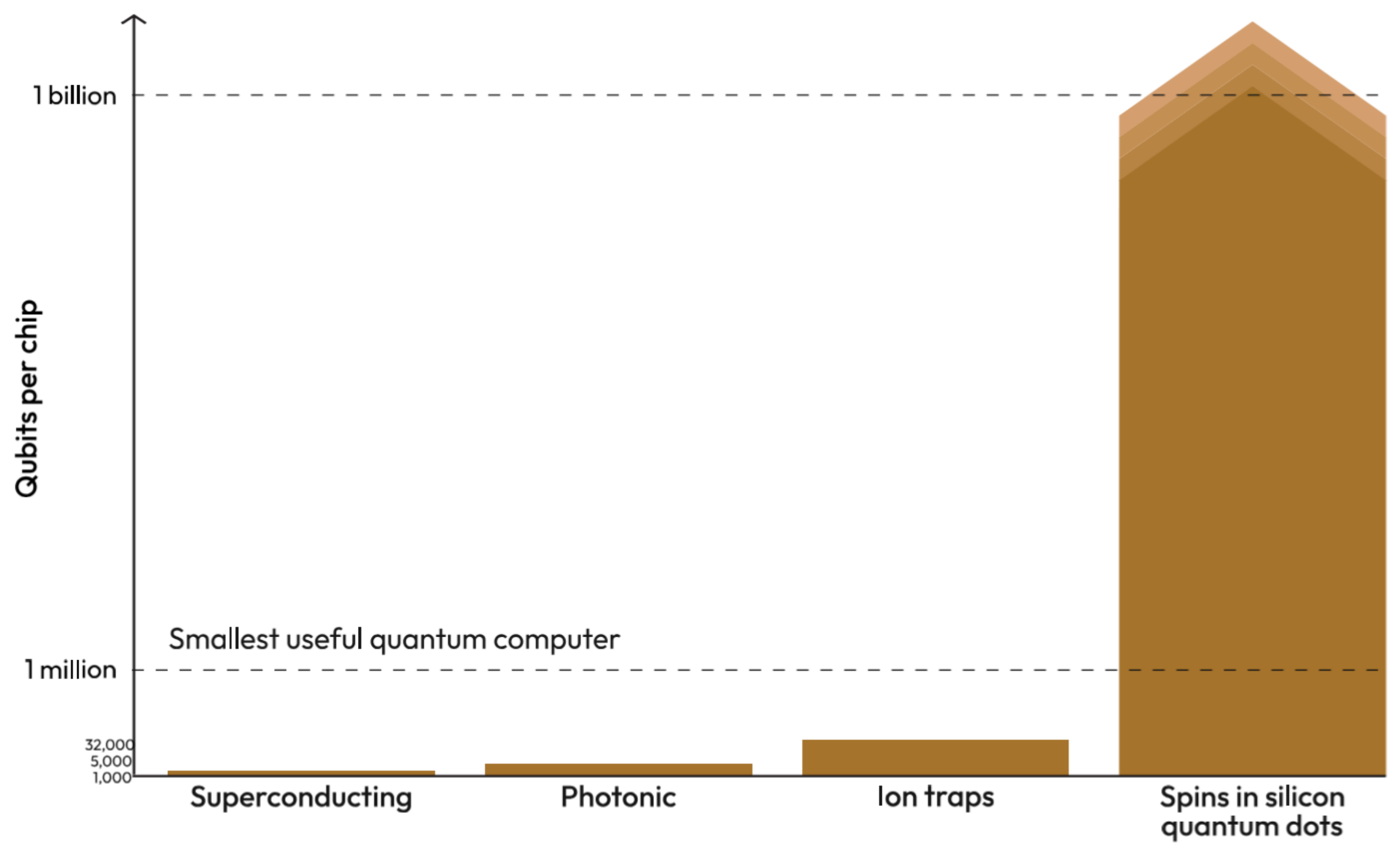
Figure 2.
Representative implementations of silicon quantum dots and arrays (gate-defined MOS/SiGe, nanowires/holes, crossbar concepts, and 2D lattices): (a–c) Few electron single, double, and triple QDs. (d) 8-site 1D QD array. (e) 3 × 3 QD array. (f,g) SiMOS single and DQD devices. (h) Donor device fabricated using STM lithography. (i) Single-layer etch defined 1 × 6 QD array in Si/SiGe. (j) 1 × 9 QD array fabricated using overlapping Al gates on Si/SiGe. (k) Enhancement mode Ge/GeSi structure. Holes are confined in (k), while the remaining devices isolate electrons. After Burkard et al., Rev. Mod. Phys. 95, 025003 (2023) [22].
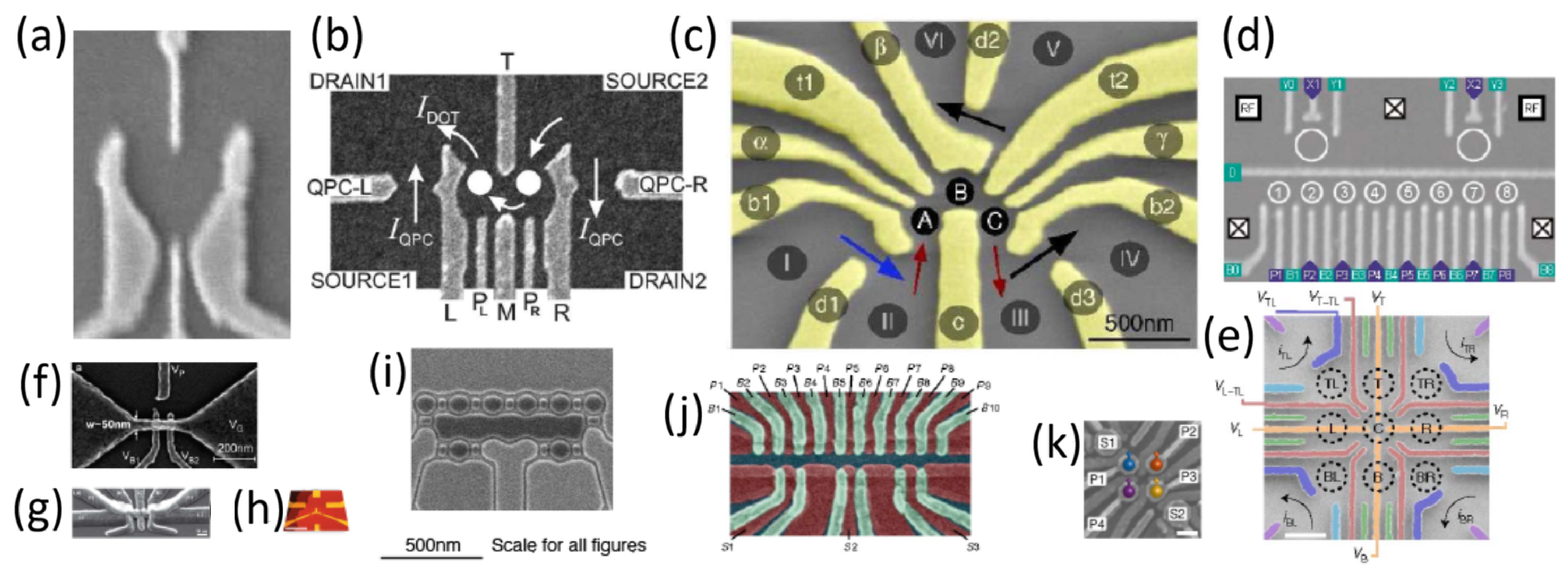
Zooming in, Figure 2 maps the concrete device landscape: gate-defined MOS and Si/SiGe quantum dots, hole-spin nanowires (Ge/Si), as well as crossbar and 2D-array layouts that enable capacitive and exchange coupling without permanent magnets. Two control knobs dominate across these realizations—detuning (on-site energies) and barrier control (tunnel coupling )—which together set the exchange interaction and hence the entangling dynamics. This architecture aligns with standard CMOS stacks and provides native access to SWAP/ primitives via time-shaped detuning and barrier pulses, paving the way for the tunable electrostatic SWAP operation analyzed next (Figure 3).
Following [23], we use a spinless tight-binding model in which on-site detuning and barrier-controlled tunnel coupling are the only electrostatic knobs. Coulomb-driven charge anticorrelation enforces single occupancy and supplies the resource for entanglement while keeping control fully capacitive—no micromagnets—thus aligning the device stack with CMOS (gate metals/oxide, mK operation, sub-10 /channel cryo-CMOS). Our numerical simulations reproduce the analytic gate-time conditions and indicate tolerance to moderate dispersion in along short chains, supporting the scalable SWAP primitive depicted in Figure 3. Various milestones to be achieved by position-based qubits are specified by Table 1.
Table 1.
Selected milestones relevant to CMOS-compatible qubits to be achieved in the near future.
Figure 3.
Basic logic elements of electrostatic position-based qubits in single-electron regime: (a)—single qubit, (b)—tunable SWAP in a CMOS-compatible DQD (double-quantum-dot) network with analytical treatment and numerical corroboration according to Pomorski [23].
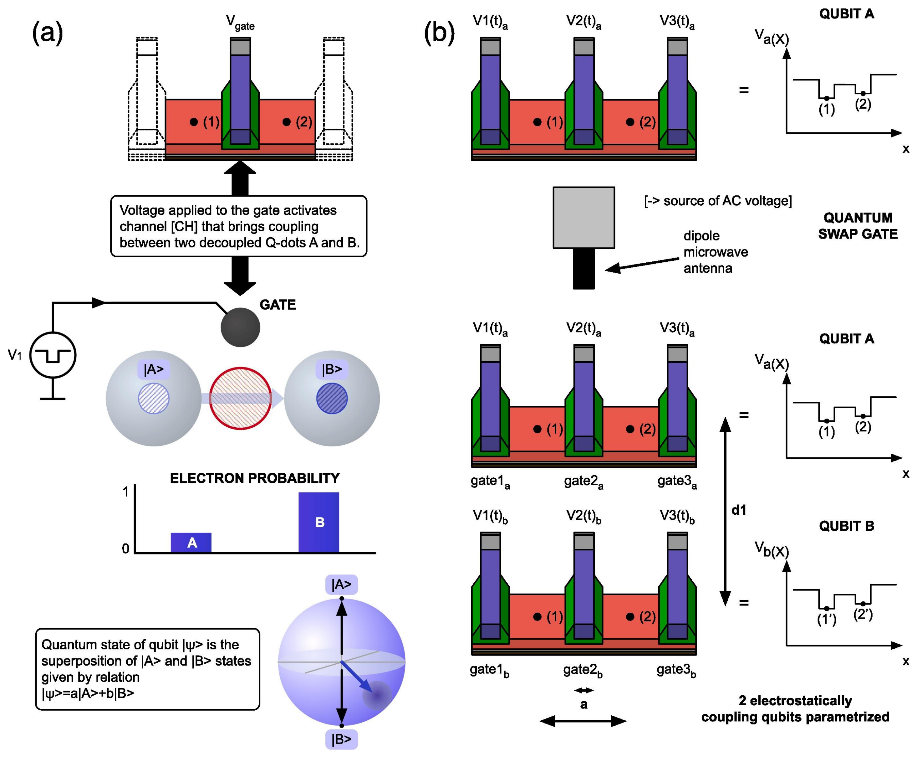
The purpose of this work is to describe position-based semiconductor qubits arranged in a chain of electrostatically controlled quantum dots using single electrons and neglecting spin, which is discussed in the preceding sections. In particular this work is the extension of previous work [23] treating the interaction of two single-electron semiconductor qubits in a more systematic way, while previous work assumed that only two position-based qubits are place in parallel at a certain distance. We also treat qubit interaction as under the influence of an external radio-frequency field. Furthermore, we provide fundamental derivation of the tight-binding model for the case of the perturbative electrostatic interaction of two qubits when they are placed at different semiconductors that are separated. We also consider a scenario in which two electrostatically interacting qubits with initially four energy levels acquire more energy levels, which violates the simplistic tight-binding model, which is important as it indicates that two interacting qubits break down after some interaction time as in Figure 4.
Figure 4.
Stages of thermalization of quantum state and evolution of occupancy of energy levels with time, represented by time arrow moving from left to right and then from top to bottom and with each lower line representing the proceeding time steps. Initially weakly interacting particles A and B are placed at two different single-electron lines, with the initial non-entangled state being the tensor product of two qubits’ quantum states and each of them having the occupancy of two energy levels. The system of two qubits starts to occupy an increasing number of energy levels, and breakdown of the tight-binding model is observed. In the meantime the emergence of quantum entanglement is observed from the initial non-entangled state as by very left bottom diagram.
2. Introduction to the Tight-Binding Model and Its Applicability in Solid-State Physics
Before using a tight-binding Hamiltonian as the main analytical tool, the manuscript needs to define the physical regime in which that approximation is meaningful. This is especially important because the work later discusses the breakdown of a reduced four-state description. The motivation of this section is therefore methodological as well as physical: to distinguish a localized-orbital, weak-overlap description appropriate for quantum-dot charge states from regimes in which delocalization, disorder, strong correlations, lattice dynamics, or self-consistent screening become essential. The section evaluates the approximation through its basis assumptions. Electrons are represented by localized atomic-like or Wannier-like states, and kinetic motion is introduced through hopping matrix elements. The discussion then tests this picture against representative failure regimes, including Mott transitions, Anderson localization, Peierls or charge-density-wave transitions, magnetic or Slater transitions, and band-overlap transitions. Table 2 summarizes why a clean, non-interacting, nearest-neighbor tight-binding model is insufficient in those cases and points toward Hubbard-type interactions, disorder models, dynamical mean-field theory, DFT+U, GW, or other first-principles approaches when the simplified basis ceases to be predictive.
Table 2.
Applicability of tight-binding model.
A central point is that delocalized eigenstates do not automatically invalidate tight binding. A periodic tight-binding model can itself produce Bloch-like states. The limitation arises when the chosen localized basis no longer gives a controlled representation of the relevant low-energy physics, for example, when orbital overlap is large, long-range hopping is important, screening changes self-consistently, or many-body interactions determine the phase. This distinction is directly relevant to the quantum-dot problem: the model is most defensible when the electron remains largely confined to a small set of dot-localized states and when the main device physics can be captured by on-site energies, tunneling, and Coulomb terms. The later observation of additional populated eigenstates is therefore a physical signal that the original truncation must be reconsidered.
The tight-binding model is adopted in this work as a controlled low-energy approximation for localized single-electron quantum-dot states, not as a universal description of solid-state electrons. Its validity depends on the persistence of a small localized basis and on limited occupation of higher orbital states. This section therefore provides the conceptual criterion used later to interpret when the model succeeds and when a beyond-tight-binding treatment is required.
The tight-binding approximation assumes that electrons’ wavefunctions can be described as linear combinations of localized atomic-like orbitals, with relatively small overlap between neighboring sites. It works best for narrow bands, localized d or f orbitals, molecular crystals, semiconductors with directional covalent bonds, and lattice models where hopping between sites is the dominant kinetic process. However, it becomes less reliable when the electronic states are strongly delocalized, as in many simple metals, where the conduction electrons resemble nearly-free Bloch waves rather than electrons bound near particular atoms.
A key point is that tight binding does not fail merely because the final eigenstates are delocalized. Even in tight binding, the eigenstates of a perfect crystal are Bloch states spread over the lattice. The failure occurs when the basis assumption becomes poor: the atomic orbitals overlap strongly, the band width is large, hopping is not limited to nearest neighbors, and the electron wavefunction is better represented by plane waves or extended Wannier functions than by localized orbitals. In such cases, a simple tight-binding Hamiltonian with fermionic electron creation/annihilation operators
may fit part of a band structure, but it no longer gives a transparent or predictive microscopic description.
For metals, especially simple s- and p-band metals, the nearly-free-electron model or first-principles band-structure methods are often more appropriate. Tight binding can still be used as an effective model if many hopping terms, several orbitals, and carefully constructed Wannier functions are included, but then it becomes a fitted representation rather than a simple physical approximation.
Metal–insulator transitions are especially problematic for the simplest tight-binding approximation because the transition is often controlled by physics that is not contained in a single-particle hopping model. A periodic non-interacting tight-binding model can describe band formation and band gaps, but it cannot generally describe the critical mechanisms responsible for real metal–insulator transitions. Important failure cases of the tight-binding model are summarized by Table 2.
For a Mott transition, the essential parameter is often the ratio , where U is the on-site Coulomb repulsion and W is the electronic bandwidth. A simple tight-binding model describes W but not the correlation physics produced by U. Therefore, it predicts a metal for a half-filled band where the real material may be an insulator. This is the classic failure behind Mott insulators and strongly correlated oxides. The Hubbard model was introduced precisely to include local electron correlations in narrow bands, beyond ordinary tight binding [24].
For Anderson localization [25], even a tight-binding lattice can be used but only after adding random site energies or random hopping amplitudes. The critical phenomenon is not ordinary band formation but the disappearance of diffusion due to disorder-induced localization of the wavefunction. Anderson’s original work showed that sufficiently strong randomness can prevent diffusion in a lattice system.
A broader review by Imada, Fujimori, and Tokura [26,27] emphasizes that metal–insulator transitions can involve correlations, disorder, lattice effects, magnetism, and orbital physics, often producing resistivity changes over many orders of magnitude. This complexity is far beyond the predictive scope of a simple non-interacting tight-binding approximation.
Thus, the tight-binding approximation should be used with caution near metallic and metal–insulator transition regimes. It is reliable when localized orbitals, weak overlap, and fixed hopping parameters are physically justified. It becomes unreliable when electrons are strongly delocalized, when screening and long-range Coulomb effects are important, when disorder controls transport, or when electron–electron and electron–lattice interactions determine whether the system is metallic or insulating. In these cases, more advanced approaches are required, such as Hubbard-type models, dynamical mean-field theory, DFT+U, GW, disorder-based localization theory, or first-principles calculations with self-consistent structural and electronic degrees of freedom. In the whole manuscript we use ; e is electron charge (Coulombs), and is the dielectric constant of vacuum.
3. Description of a Position-Based Qubit in the Tight-Binding Model
The goal of this section is to define the elementary qubit used throughout the manuscript: one electron shared between two neighboring quantum dots, with logical information encoded in position. A mathematically explicit single-qubit description is required before Coulomb-coupled two-qubit gates can be analyzed. The section therefore establishes how experimentally meaningful controls—local electrostatic energies and interdot tunneling—enter the qubit Hamiltonian and how those parameters determine coherent state evolution. A two-state tight-binding Hamiltonian is written in the localized position basis using the on-site energies and and the generally complex tunneling amplitude . The same system is also represented in its instantaneous energy eigenbasis. Analytical expressions are introduced for the eigenenergies and eigenstates, followed by the Schrödinger time-evolution equation, the unitary propagator, and the density-matrix representation. A Pauli-matrix decomposition is then used to connect the Hamiltonian to the standard two-level formalism. Special limits—vanishing hopping, dominant hopping, and asymmetric on-site energies—are considered to show how the propagator depends on the physical control parameters.
This construction identifies the two quantities that play the role of primary control axes in the position-basis qubit: energy detuning biases localization, while the hopping term produces coherent transfer between the dots. The model makes the relation between voltage control and qubit dynamics transparent because both quantities can, in principle, be modified electrostatically. The density-matrix formulation is important for the later two-qubit discussion because it provides the natural route to occupation probabilities, coherences, and entanglement measures. The analytical propagators are most useful when the effective two-state basis remains valid; if additional orbital states become appreciably populated, and should be regarded as effective parameters of a truncated model rather than complete microscopic descriptors.
Section 3 supplies the single-qubit building block for the entire manuscript. It defines the localized basis, energy basis, Hamiltonian parameters, unitary dynamics, and density-matrix language that are reused for coupled devices. In physical terms, it shows how a double quantum dot can function as a voltage-controlled position qubit whose coherent evolution is governed by detuning and tunneling.
We are motivated by the methodology given in work [28]. We refer to the physical situation from Figure 5 as given by [29,30,31,32,33], and we consider a position-based qubit in the tight-binding model [33] Hamiltonian or in energy bases as given by
The Hamiltonian eigenenergies and with are given as
and energy eigenstates and have the following form
This Hamiltonian gives a description of two coupled quantum wells as depicted in Figure 5. In such a situation we have real-valued functions , and complex-valued functions and , which is equivalent to the knowledge of four real-valued time-dependent continuous or discontinuous functions , , and . The quantum state is a superposition of state localized at nodes 1 and 2 and therefore is given as
where () is the probability of finding a particle at node 1 (2), which brings and obviously and . In the Schrödinger formalism, states and are Wannier functions that are parameterized by position x. We work in tight-binding approximation and quantum state evolution with time as given by
The last equation has an analytic solution
and in quantum density-matrix theory we obtain
Pauli Decomposition Applied to Tight-Binding Hamiltonian
Any Hermitian matrix admits the expansion with and . For composite systems, can be written as , where and .
Using the above property for matrix of size 2×2 we obtain and assuming and we are given matrix
where (.) and (.) are sinh and cosh hyperbolic functions, where . This matrix is unitary, so . At the very end we will also consider a more general case when . At first let us consider the case of two localized states in the left and right quantum wells so there is no hopping, which implies . In such a case the evolution matrix is unitarian and has the following form
which implies that the left and right quantum dots are two disconnected systems, each undergoing its own time evolution. However since one electron is distributed between those physical systems the measurement conducted on the left quantum dot immediately affects the right quantum dot. Another extreme example is the situation where hopping energy is considerably bigger than localization energy. In such a case we set , and in the case of non-zero hopping terms we obtain given below
Now it is time to move to the most general situation of , . We have four elements of the evolution matrix given as
Figure 5.
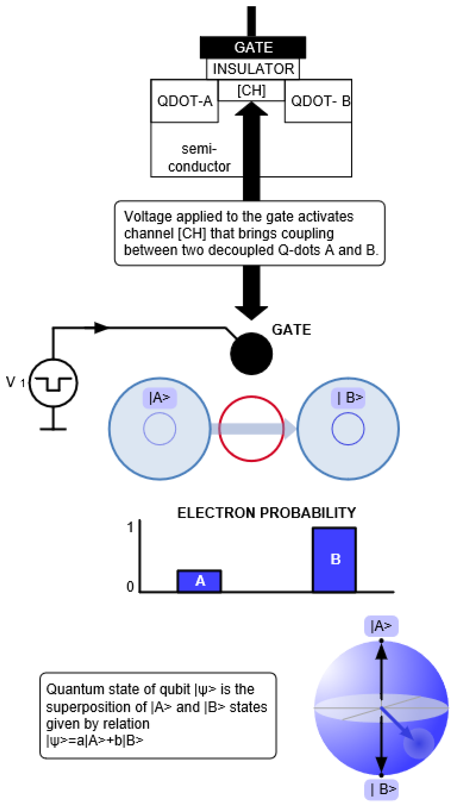
Scheme of electrostatically controlled qubit made from two neighboring quantum dots and referring to Figure 3 showing implementation of the single qubit.
4. Description of Two-Qubit Interaction in the General Static Case
The main scientific step of the work is the transition from one position-based qubit to two electrostatically interacting qubits. In case of many interacting particles one can use mapping between quantum mechanics and statistical physics [34]. A two-qubit model is necessary to describe SWAP-like dynamics, Coulomb-driven correlation and anticorrelation, and the generation of entanglement. The motivation of this section is therefore to construct the smallest Hamiltonian that retains the relevant device ingredients while remaining sufficiently compact for analytical treatment. Two double quantum dots, labeled as upper and lower qubits, are represented in a four-state product basis. The Hamiltonian contains the local confinement energies of both qubits, their individual tunneling amplitudes, and four geometry-dependent Coulomb energies associated with the possible electron-position configurations. The matrix is also decomposed into the tensor products of Pauli operators. Analytical expressions for unitary evolution are developed for selected parameter restrictions, while eigenenergy spectra are studied as functions of distance and hopping. The symmetric Q-SWAP subsection specializes the model to equal on-site potentials and equal tunnel couplings, allowing explicit discussion of entangled eigenstates, degeneracy, correlation structure, and perturbative transitions between energy levels.
The physical content of the four-state model is the competition among three mechanisms: localization by electrostatic bias, coherent redistribution by tunneling, and configuration-dependent energy shifts produced by Coulomb repulsion. Coulomb repulsion alone favors particular charge configurations, but a quantum gate requires coherent superpositions and therefore depends essentially on the tunneling terms. The symmetric case provides transparent analytical insight, yet the general Hamiltonian is more important for realistic devices because interdot distances, local biases, and couplings are not perfectly identical. The manuscript also connects entanglement to measurable charge correlations and to the von Neumann entropy, which gives the analytical formalism a possible experimental interpretation through charge-state readout.
This section establishes the general two-qubit electrostatic Hamiltonian and shows how SWAP-related behavior emerges from the combined action of tunneling and Coulomb interaction. The symmetric solution serves as a useful reference point, while the more general parameterization supplies design variables for nonideal geometries. It also defines the correlation and entanglement quantities used in later sections to characterize gate operation.
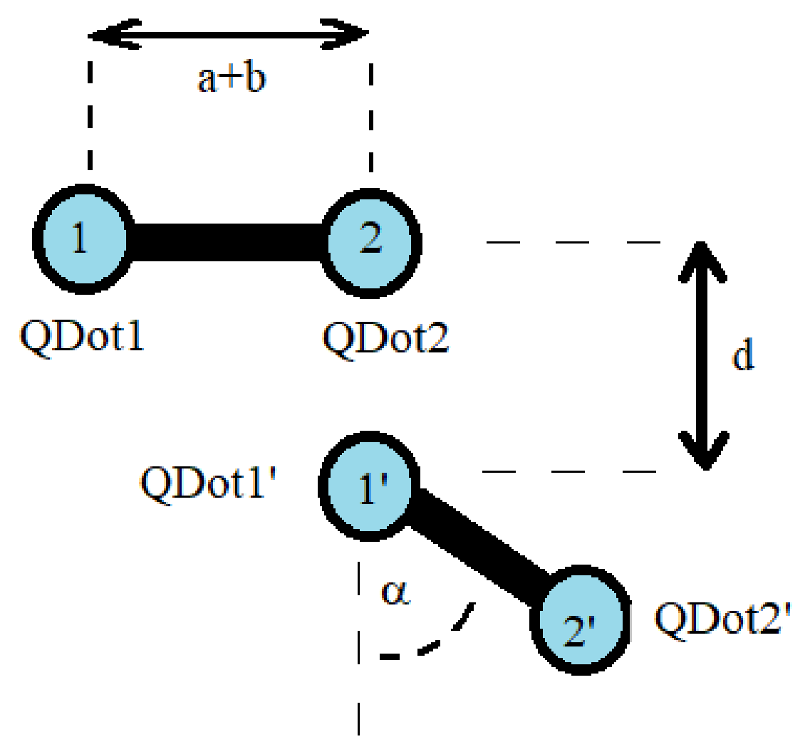
We consider the most minimalist model of two electrostatically interacting position-based qubits, which are double quantum dots A (with nodes 1 and 2 and named U-upper qubit) and B (with nodes 1′ and 2′ and named L-lower qubit), with local confinement potentials as given in Figure 6 and Figure 7. By introducing notation the minimalistic Hamiltonian of the system of electrostatically interacting position-based qubits can be written as
described by parameters , , , , , and distances between nodes k and l’: , , , . In such a case the q-state of the system is given as
where the normalization condition gives . The probability of finding an electron in the upper system at node 1 is determined by the action of the projection on q-state , so it gives probability amplitude . On the other hand the probability of finding an electron from qubit A (U) at node 2 and an electron from qubit B(L) at node 1 is obtained by the projection acting on the q-state giving that gives probability amplitude . Referring to Figure 6 we set distances between nodes as , and assume the Coulomb electrostatic energy to be of the form , and hence we obtain the matrix Hamiltonian given as
We can introduce notation and . In the most general case of 2-qubit electrostatic interaction, one qubit has four different Coulomb terms on matrix diagonal , , , and . We introduce , , , and in such a case by using Formula (8) one can decompose the two-particle Hamiltonian as
A very similar procedure is for the case of three or N interacting particles concerning the tensor product of three or N Pauli matrices. In order to simplify the representation of the unitary matrix describing the physical system of the evolution of the two particles with time it is helpful to define , , , and , . We consider the situation where there is no hopping between q-wells , so the second particle is localized among two quantum wells, and the first particle can move freely among 2 q-wells. We obtain the following unitary matrix evolution with time with and
Figure 6.
Scheme of electrostatic quantum gate as two interacting qubits ([23,32,33,35,36]) with geometric parametrization of generalized electrostatic quantum gate.
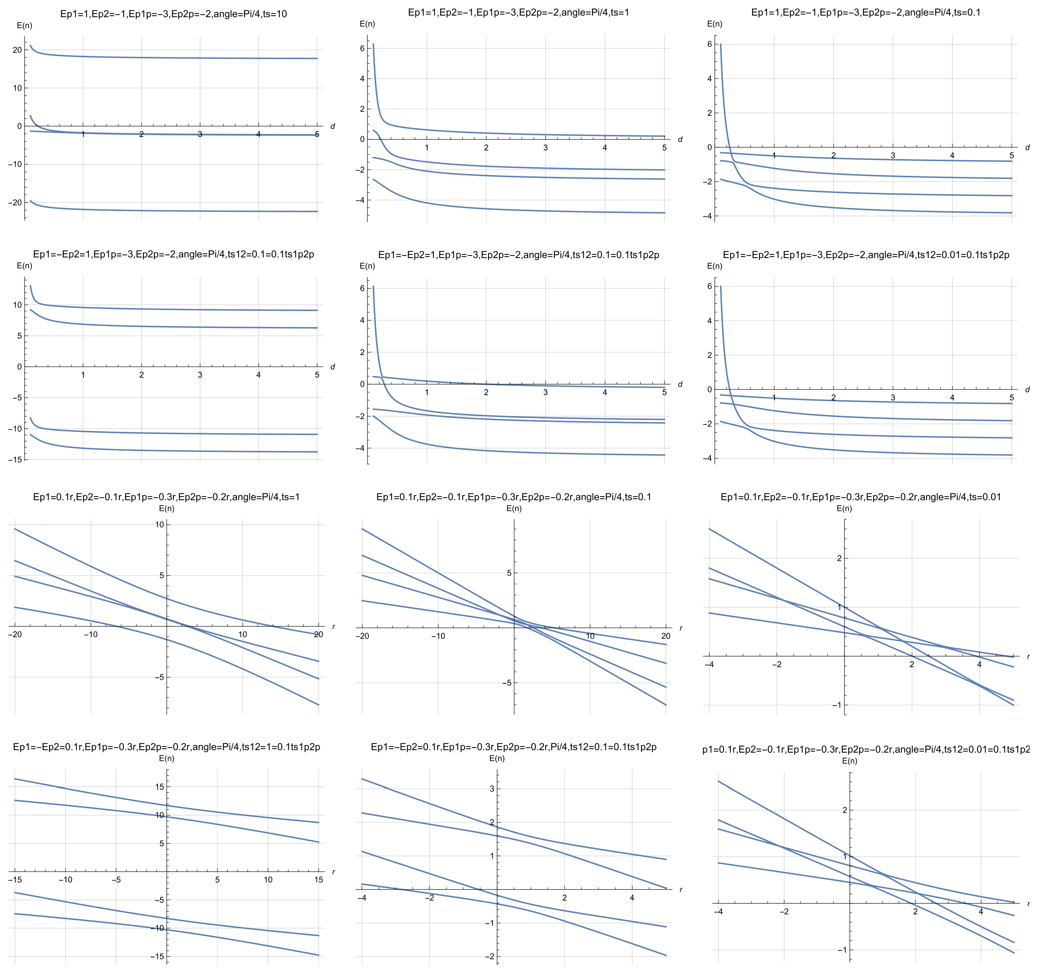
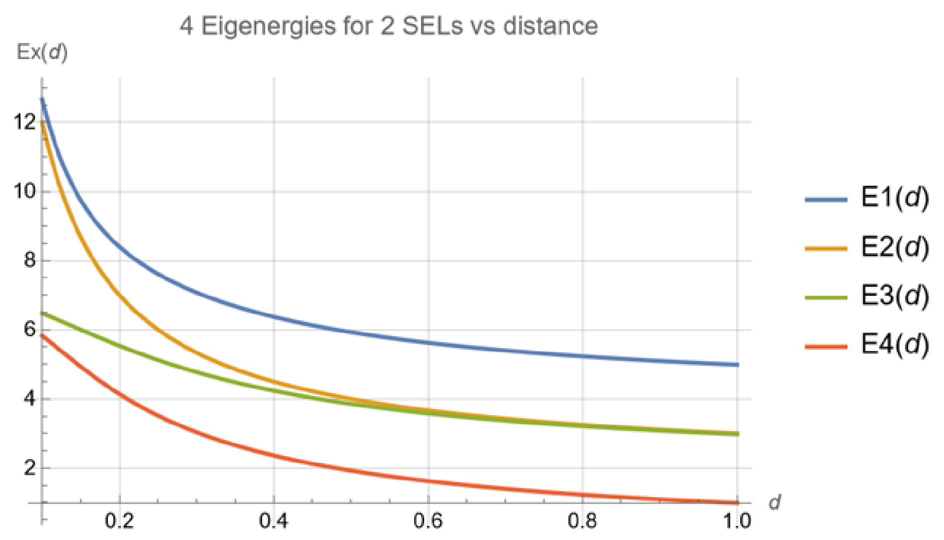
The example of function dependence of eigenenergy spectra of two electrostatically interacting qubits on distance is given by Figure 8.
An important observation is that any element of matrix for denoted as is transferred to element of matrix . We can easily generalize the presented reasoning for the system of N electrostatically coupled electrons confined by some local potentials. However we need to know the position-dependent Hamiltonian eigenstate at the initial time . In case finding such an eigenstate is the numerical problem since analytical solutions for roots of polynomials of one variable for a higher order than 4 do not exist. Using the numerical eigenstate at time instance we can compute the system quantum dynamics in an analytical way. This gives us a strong and relatively simple mathematical tool allowing full determination of the quantum dynamical state at any instance of time. The act of measurement on the position-based qubit is represented by the operator and .
Figure 7.
From (left) to (right): anticorrelation principle in the Q-SWAP gate; scheme of the renormalization procedure in a system of coupled qubits, following the procedure given in the work by K. Pomorski entitled “Analytic view on N-body interaction in electrostatic quantum gates and decoherence effects in the tight-binding model” [36]; illustration of the anticorrelation principle in a classical or quantum SWAP gate; correlation principle in a chain of coupled dots aligned along one line or along parallel lines; correlation principle for a system of qubits in perpendicular alignment. This last system is also equivalent to the generalized electrostatic quantum SWAP gate from Figure 6.
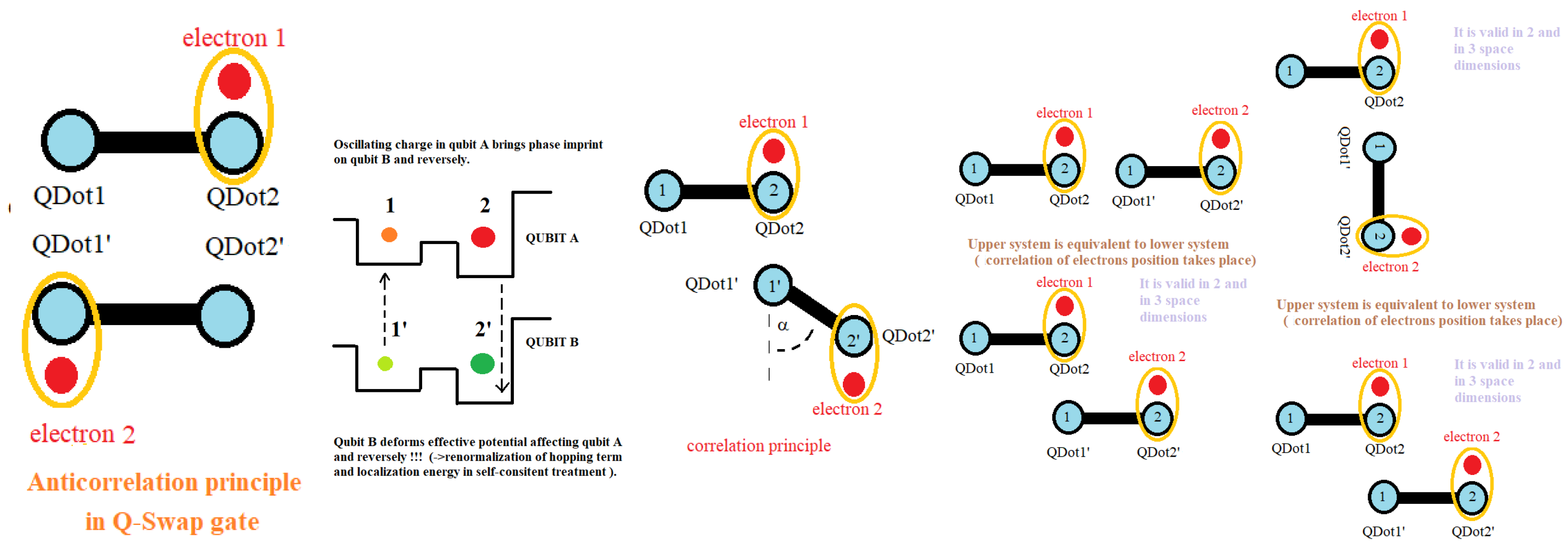
Figure 8.
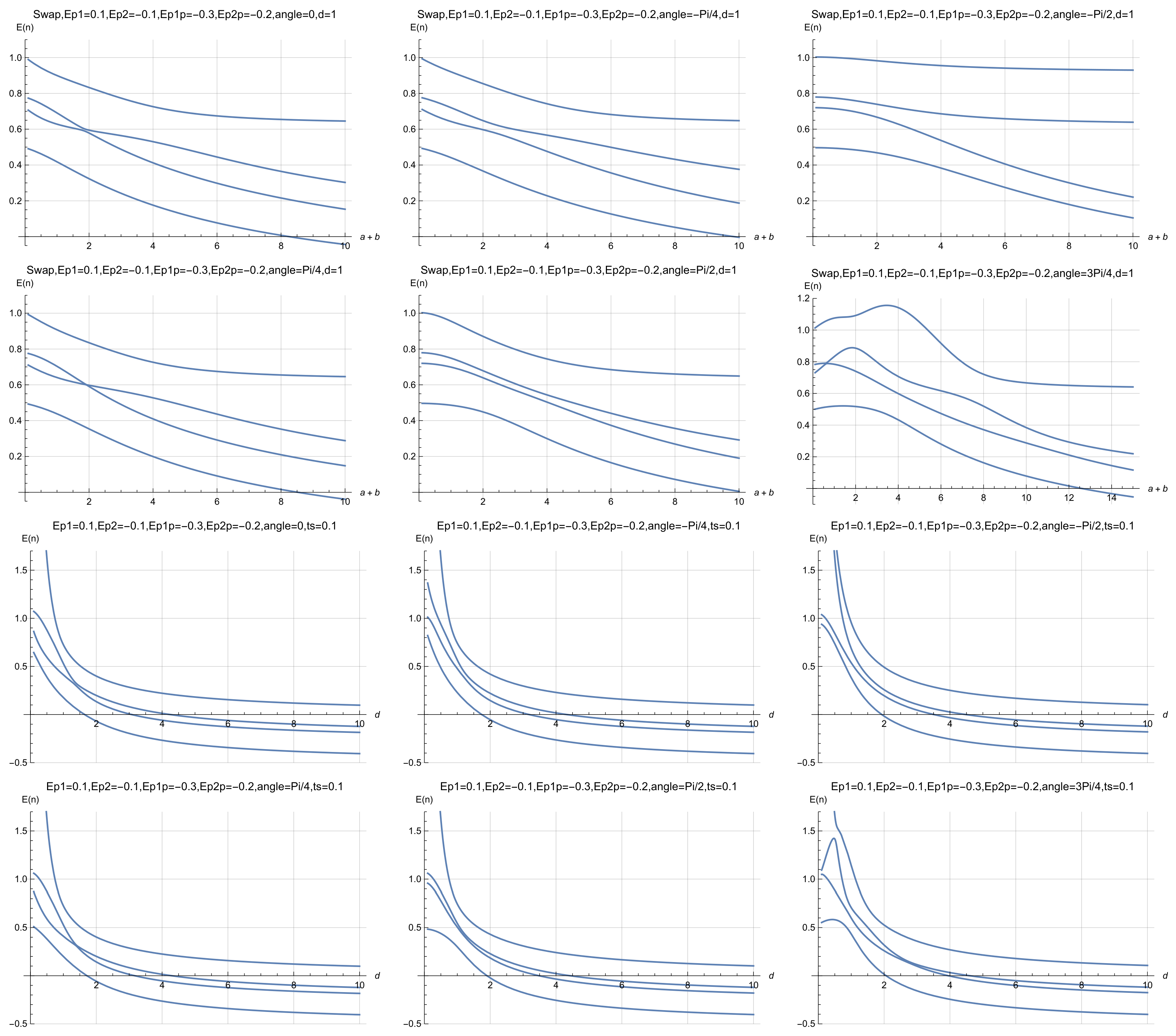
Case of metal–insulator-like transition, interpreted as a transition from delocalized to more localized electronic states caused by decreasing the hopping term value, as seen from the energy spectra of the quantum SWAP gate as a function of the distance d for the case of two electrostatically interacting qubits shown in Figure 6. No level crossings are observed, even after careful magnification of the plots.
Simplified Picture of a Symmetric Q-SWAP Gate
Now we need to find a system of four eigenvalues and eigenstates (four orthogonal 4-dimensional vectors), so we are dealing with a matrix eigenvalue problem), a standard topic in linear algebra. Let us assume that two double-quantum-dot systems are symmetric and biased by the same voltages generating potential bottoms so we have and . Denoting and we obtain four orthogonal Hamiltonian eigenvectors
We observe that the first two energetic states are degenerated, so the same quantum state corresponds to two different eigenenergies and . This degeneracy is non-present if we come back to the Schrödinger picture and observe that localized energy and hopping terms for one particle are dependent on the presence of another particle, which leads to renormalization of wavevectors. The situation is depicted in Figure 7. The degeneracy of the eigenstates is lifted if we set , and ,
.
The same argument for another wavevector is given below.
where c = . The first two and energy eigenstates are always entangled, while and eigenenergies are only partially entangled if . If , the last two energy eigenstates are not entangled. The situation of c=1 takes place when , when two qubits are infinitely far away and thus electrostatically decoupled. The situation of c=0 is interesting because it means that and are maximally entangled, and it occurs when , so when two electrons are maximally localized in each of the qubits so there is no hopping between the left and right wells.
The obtained eigenenergy states correspond to four eigenenergies
We also notice that the eigenenergy states , , , and do not have classical counterparts since an upper electron exists at both positions 1 and 2 and a lower electron exists at both positions at the same time. We observe that when the distance between two systems of double quantum dots goes to infinity the energy difference between the quantum state corresponding to and goes to zero. This makes those two entangled states degenerated.
Four normalized eigenvectors of two interacting qubits in the SWAP Q-Gate configuration are of the following form
We are obtaining simplifications after assuming , so we obtain
It is worth mentioning that if we want to bring two electrostatic qubits to the entangled state we need to cool down (or heat up) the system of interacting qubits to the energy (or to energy ). Otherwise we might also wish to disentangle two electrostatically interacting qubits. In this way, one of the scenarios is to bring the quantum system either to energy or so only partial entanglement is achieved. The other scenario would be introducing the occupancy of different energetic levels so the net entanglement is reduced. One can use the entanglement witness in quantifying the existence of entanglement. One of the simplest forms of q-state entanglement measurement is von Neumann entanglement entropy as expressed by Formula (A139), which requires the knowledge of q-system density matrix with time. Such matrices can be obtained analytically for the case of two electrostatically interacting qubits.
It is interesting to note the dependence of eigenenergies on distance between interacting qubits in the general case as depicted in Figure 7. Now we are moving toward description the procedure of cooling down or heating up in the Q-SWAP gate. The procedure was discussed previously in the case of a single qubit. Now it is exercised in the case of 2-qubit electrostatic interaction. For the sake of simplicity we change the occupancy of the energy level and energy level level and keep the occupancy of other energy levels unchanged. We can write the as
We introduce and real-valued functions of small magnitude , and we consider the following Hamiltonian with that has part of time-independent and part of time-dependent as
Initially we establish the following parameters of the tight-binding model as . Changing into and into while keeping other parameters of the tight-binding model unchanged results in the heating up (cooling down) of the q-state of the SWAP gate, so the population of energy levels and is time-dependent, while populations of energy levels and are unchanged. Practically our results mean that we need to keep all our confinement potential bottoms constant while changing the barrier height between neighboring q-dots in each of the position-based qubits. In this way we establish the procedure of perturbative cooling (heating up) of the q-state. A non-perturbative approach is absolutely possible, but it requires full knowledge of time-dependent eigenstates and eigenenergies (solutions of eigenenergies of fourth-order polynomials are very lengthy in the general case), and therefore corresponding expressions are very lengthy. In similar fashion we can heat up or cool down two coupled single-electron lines [33] as in Figure 6 and Figure 7 or any other q-system with N interacting q-bodies that can be represented by the system of N-interacting position-based qubits.
5. Quasiclassical Approach Toward a Tunable SWAP Gate
The fully quantum Hamiltonian gives the most complete low-energy description, but it can obscure the intuitive electrostatic conditions that favor one logical configuration over another. This section introduces a quasiclassical viewpoint to obtain direct design rules for a tunable SWAP gate. The objective is to understand how gate geometry and localizing potentials determine whether correlated or anticorrelated charge configurations are energetically preferred before coherent quantum dynamics is added. The analysis suppresses or strongly reduces the kinetic contribution by considering the limit of small tunneling. The resulting energy is written as a function of the occupation probabilities of the two qubits, the local electrostatic potentials, the interdot distances, and a geometric angle . Symmetric and asymmetric configurations are compared by assigning energies and to different logical charge arrangements and deriving inequalities that determine the energetically favorable states. The subsection on the transition from an anticorrelated symmetric SWAP gate to a correlated gate uses this energy landscape to show how changing geometry and bias can move the system between operating regimes.
The value of the quasiclassical model is not that it replaces the quantum description but that it separates electrostatic design from coherent dynamics. It shows which charge configurations are selected by Coulomb-energy minimization and therefore identifies the regions in parameter space where a quantum tunneling term can act on an already favorable electrostatic landscape. This creates a useful bridge between lithographic geometry, gate voltages, and the qualitative form of the two-qubit interaction. At the same time, because kinetic energy and coherence are reduced in this treatment, the quasiclassical energy minima should be interpreted as design guidance rather than as a complete prediction of entangling-gate fidelity or coherent time evolution.
Section 5 provides a device-oriented tuning picture for the electrostatic SWAP architecture. By expressing the gate energy in terms of occupations, biases, distances, and relative geometry, it identifies conditions that favor correlated or anticorrelated configurations. These conditions complement the quantum model by translating the Hamiltonian into practical electrostatic design rules.
5.1. Quasiclassical Approach Toward a Symmetric SWAP Gate with the Same Localizing Potentials
We assume that one particle is in the field of another particle that is given by integro-differential equations as often used in quantum chemistry. In addition we assume that the kinetic energy of particles A and B (electrons in qubits A and B) is very small, so and ; however, still and , so after a certain length of time particles have the chance to find a proper configuration. We assume that is the probability of finding particle A at node 1 and that is the probability of finding particle B at node 1′. We have an effective Hamiltonian omitting kinetic terms in the form
The well-designed classical SWAP and Q-SWAP gates (inverting states 0 to 1 and 1 to 0) have the property that the function reaches its minima at and at and that . Consequently we assume
- and
- ,
- which implies that logical states that are not allowed have higher energy. Further simplification can be done by setting, for example, and to a constant value (as and ), for example, 0 or 1 or any other fixed real number. It is underlined that we can choose the one among four possible combinations , , , whose values need to be fixed. We set , , , . We obtain
5.2. Transition from an Anticorrelated Symmetric SWAP Gate to a Correlated SWAP Gate
We have an effective Hamiltonian omitting kinetic terms for any angle in the form
The previously considered case was for the angle that corresponds to the symmetric anticorrelated SWAP gate as specified by Formula (32). Let us set and to be 1. We obtain the following values as
with condition that implies
and we obtain
We can check the designing condition that implies
and consequently we obtain
which brings the condition
that is equivalent to the condition or where . The presented considerations are visualized by Figure 9 and Figure 18, which describes the dependence of the phenomenological electrostatic Hamiltonian on logical values and , which enables a construction fuzzy logic SWAP gate or quantum SWAP gate to be implemented in single-electron devices.
Figure 9.
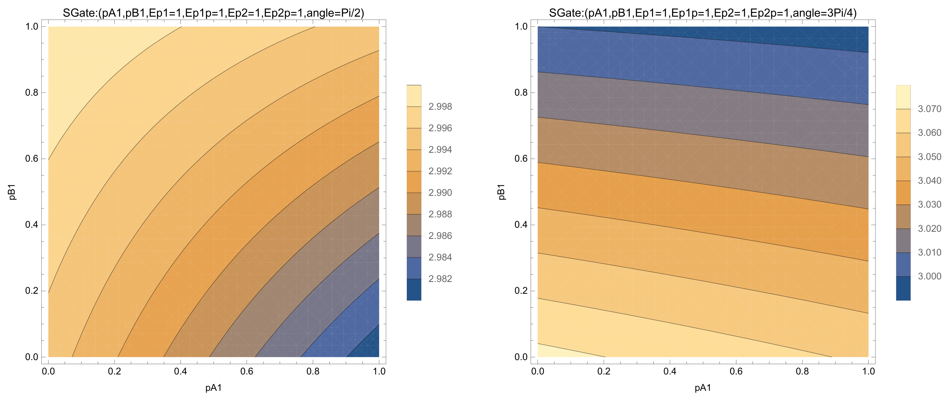
Transition from the classical/quantum SWAP gate into the ANTISWAP gate by changing the angle from to . Minima in phenomenological Hamiltonian identifies the preferable logical state (states of () and () are preferred in the same way) into only one preferred state (). Contour plots describing qubit–qubit Hamiltonian values in function of probabilities (, ) of SWAP and ANTISWAP gates were magnified.
6. Electrostatic Quantum ANTISWAP Gate
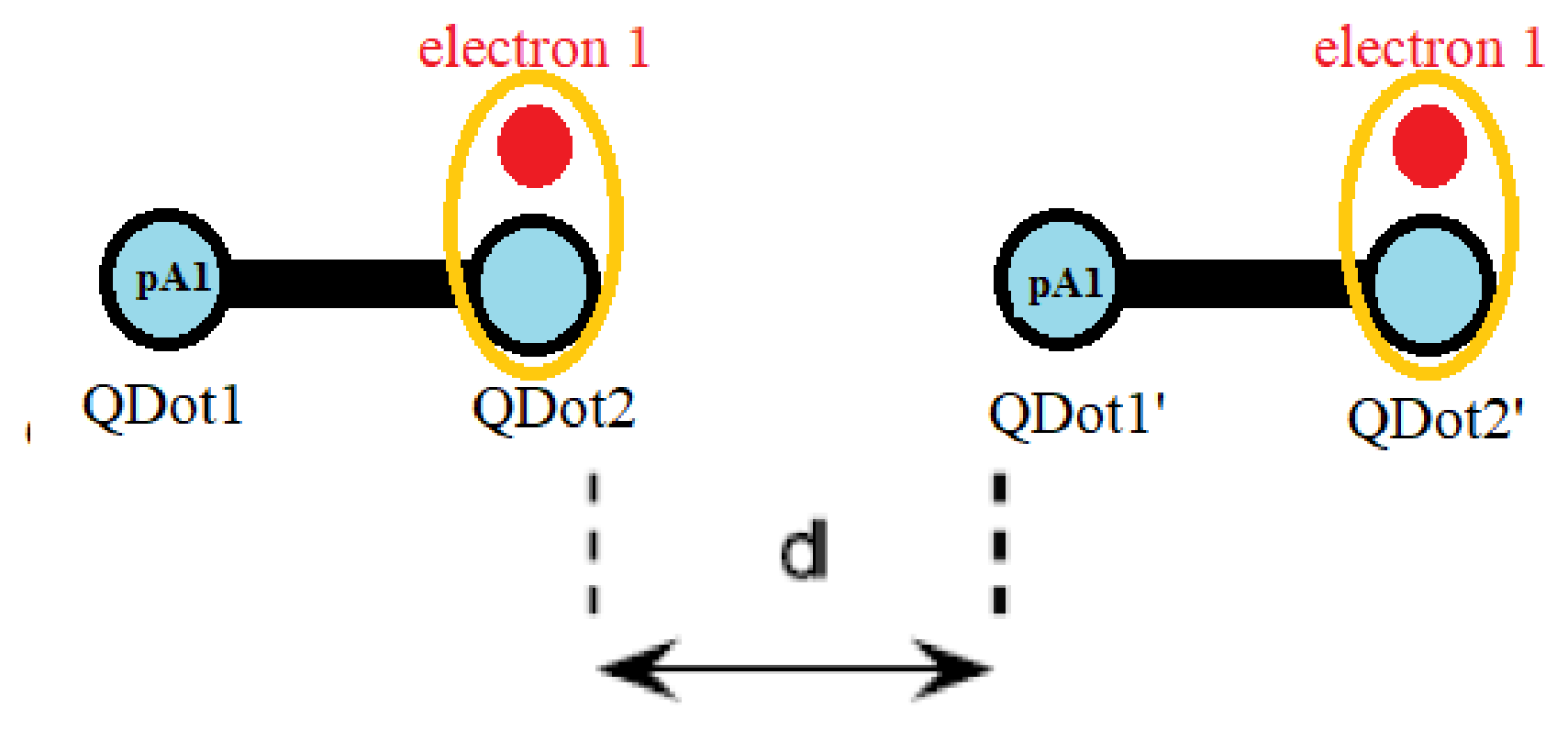
This section explores a complementary operating regime in which the two charge qubits described in tight-binding model are driven toward correlated and later anticorrelated occupancy as depicted in Figure 10. In meantime the quasi-classical SWAP-gate Hamiltonian on the electrostatically controlled polarizing potentials is depicted in the figure. Consequently later the manuscript describes tight-binding regime known as an electrostatic ANTISWAP or repeater-like operation as depicted in figures. Its motivation is to show that the same coupled-dot hardware can support more than one logical response, depending on the chosen geometry and bias conditions. The section starts from the occupation-dependent electrostatic Hamiltonian and selects local potentials such that equal or related charge configurations become energetically favorable. The energies of the relevant logical states are grouped into and , and algebraic conditions are derived for the ordering . The analysis relates those inequalities to the interdot distance, the dot separation , and the local confinement energies. This produces explicit voltage and geometry conditions under which the correlated operating point is preferred.
The important scientific point is the tunability of the interaction sign at the level of charge-state preference. By changing the electrostatic energy landscape, the device can favor anticorrelated states associated with the SWAP-like configuration or correlated states associated with the ANTISWAP/repeater-like configuration discussed here. This reinforces the manuscript’s broader claim that the logical behavior is encoded not in a single fixed coupling constant but in a combination of geometry, confinement energies, and tunneling. The section is most naturally interpreted as a model of controllable charge-state correlation within the restricted two-level description.
The ANTISWAP analysis demonstrates that electrostatic design can select a correlated operating regime in the same family of double-dot structures used for the SWAP gate. The derived inequalities provide a direct prescription for choosing local potentials and geometry so that the desired logical charge configurations have lower energy than competing states.
We can use the fact that two qubits can be in maximum correlated states (if we have ). Due to repulsive electrostatic interaction we can build the electrostatic quantum ANTISWAP gate so it corresponds to the situation where one qubits is being copied by another qubit. It is underlined that the same considerations apply for the electron-hole system () and hole-hole system ().
Figure 10.
Scheme of electrostatic ANTISWAP gate.
We have
We set and we have
In order to obtain the quantum repeater we have , and such a configuration is energetically favorable (minimizes Hamiltonian energy) so we have
We have the condition
and it implies . We have
We have
and it implies
where
since and , so condition is fulfilled.
In the next section, we present a fundamental derivation of the tight-binding model from the Schrödinger equation.
7. From Eigenenergy Qubits to Position-Based Qubits
A position-based qubit is convenient for describing a physical double quantum dot, whereas many quantum-control formalisms are written in an energy eigenbasis. This section is motivated by the need to connect these two representations without changing the underlying quantum state. Establishing that connection is essential for translating between abstract qubit amplitudes, localized charge probabilities, and experimentally tunable device parameters. The section introduces a rotation between the energy-basis Hamiltonian and the position-basis Hamiltonian . A mixing angle is used to construct maximally localized Wannier-like left and right states from the two lowest-energy eigenstates. Matrix elements of the microscopic Schrödinger Hamiltonian are then projected into the localized basis to identify the effective on-site energies and tunneling terms. The development also treats asymmetric cases and uses the same mapping to express occupation probabilities and electrostatic gate energies in either representation.
This basis transformation clarifies that the energy and position descriptions are not competing physical models when they span the same two-dimensional subspace. They are different coordinate systems for the same truncated quantum dynamics. The position basis is especially useful for semiconductor devices because charge sensing and gate voltages are naturally local, while the energy basis is useful for spectral analysis and control protocols. The manuscript also emphasizes that the mapping relies on a well-defined two-level subspace and on localized Wannier functions. If higher levels become populated, a two-state rotation is no longer sufficient, and the effective parameters must be generalized.
Section 7 provides the formal bridge between abstract eigenenergy qubits and the localized charge qubits used in the proposed CMOS-compatible architecture. It shows how energy eigenstates, localized Wannier states, confinement energies, and hopping amplitudes can be transformed into one another within the two-level approximation.
The Hamiltonian of the tight-binding model describing single-electron devices (as presented by Fujisawa [29] or Pomorski [37]) uses the Hamiltonian of position-based qubit with rotation matrix , fictitious angle and eigenenergy Hamiltonian . In the case of the two-energy-level system, this can be expressed in the following form:
We continue elementary mathematical steps
where we use the property of maximization of the presence of the left Wannier wavefunction in the region from to encoded in minimization of functional , so is achieved. Having the logical state zero assigned from to (medium distance between two quantum dots) we obtain the formula for angle as given by [37] and the expression
It is useful to parameterize by the introduced quantity and two eigenenergies and . It is proper to underline that
Consequently using the fact that is time-independent we obtain the following chain of equivalent expressions giving the transformation from the energy base to the position base
where we introduce the complex value function expressed as a linear combination of maximal localized Wannier functions localized on the left or on the right side ( and ) or as a linear combination of the two lowest-energy eigenstates and with effective potential describing a position-based qubit in the single-electron regime as depicted in Figure 5 and Figure 6. We assume that this potential is only weakly time-dependent.
We observe that a given quantum system expressing single-electron qubits can be described by eigenenergy Hamiltonian , and this picture can be transferred into position-based Hamiltonian or reversely. A detailed case with two symmetric conditions for two interacting qubits in effective tight-binding Hamiltonian with respect to diagonal terms is given in Appendix C, when
Another cases of analytic treatment of two interacting qubits in asymmetric case is treated by Appendix D
An example of introduction of correlation/anticorrelation (simultaneous position of electrons on the same/opposite site) function
for two interacting qubits is treated by Appendix E. With solutions of the tight-binding model for static electric fields coming from qubit-position biasing gates we can explore the cases with the presence of an EM field, which will be done in the next sections. At first we investigate the tight-binding model from the point of view of self-consistency using the Schrödinger formalism.
8. Higher-Order Effects and a Picture Beyond the Tight-Binding Model
The earlier sections deliberately use a reduced tight-binding description. Section 8 asks whether that truncation remains self-consistent when two qubits interact for finite time and when external electromagnetic driving or radiative processes are included. The motivation is therefore to identify physical effects that cannot be captured indefinitely by a four-state model and to determine when a more microscopic Schrödinger description becomes necessary. The manuscript treats the Coulomb interaction between two confined electrons as a perturbation to the dominant single-particle confinement and follows the resulting two-body wavefunction in time. The analysis compares the evolution predicted by the reduced tight-binding picture with a perturbative Schrödinger treatment. The subsection on entangled two-photon emission considers transitions between interacting states and discusses how gate-voltage patterns could be optimized to enhance correlated radiative channels. The thermalization subsection tracks the redistribution of state occupation and the growth of entanglement, with Figure 4 and Figure 11 used to illustrate the appearance of additional energetic components and the evolution from initially separable to more entangled states.
Figure 11.
Partial correspondence between a four-resonator photonic network and two electrostatically interacting single-electron lines as given by [38] and also by [39]. Similarly [40] presents resonant microwave-mediated interactions between distant electron spins. One can also place the physical system [12] among pointed resonant cavities [41] that will have coherent charge oscillations in a silicon nanowire double quantum dot by gate-based radio-frequency dispersive sensing.
This is the key limitation analysis of the manuscript. The central observation is that a system initially represented by two levels per qubit can populate additional eigenstates as the interaction evolves. In that regime, fixed effective values of and cease to provide a complete description; their apparent time dependence reflects the fact that the reduced basis is absorbing physics from degrees of freedom that were omitted. The section therefore distinguishes a short-time, low-energy regime in which tight binding is useful from longer-time or more strongly driven conditions where a larger basis is required. The photon-emission discussion also broadens the role of the coupled-dot system from purely logical gating toward possible interfaces with electromagnetic degrees of freedom.
Section 8 shows that the tight-binding model is a useful first approximation but not a closed description at arbitrary time scales. The perturbative Schrödinger analysis provides evidence for higher-state occupation and increasing entanglement, which marks the onset of a beyond-tight-binding regime. This result is essential for interpreting all preceding analytical gate formulas as low-energy, finite-validity descriptions rather than universal dynamics.
One particle is moving in the electric field of another particle that corresponds to the case of the Hamiltonian with a more prominent time-independent part and small time-dependent part.
We give the Schrödinger equation for the system of two interacting particles in the regime of small particle–particle interaction subjected to time-dependent electric biasing of metallic gates and thus having the form
where and are effective potential for confined electrons for qubits A and B, so they have two minima for each separated qubits A and B with the presence of mutual qubit–qubit interaction given by . At first we refer to the situation of a toy model of two qubits with the occupancy of two energy levels each as for systems A and B and with the situation of weak qubit electrostatic interaction.
We go beyond results given in [42,43] and we have the following cases under the assumption that the time-dependent component of the Hamiltonian is of perturbative character:
- , with no photon emission or absorption in neither qubit;
- , with possible photon emission or absorption in qubit B;
- , with possible photon emission or absorption in qubit A;
- , due to mutual qubit–qubit interaction (with the possibility of photon emission or absorption by each of qubits A and B);
- , with simultaneous photon emission (as in the case of entangled photon emission) by qubits A and B;
- , with simultaneous photon absorption (as in the case of entangled photon emission) by qubits A and B;
- , with photon emission by qubit A;
- , with photon emission by qubit B.
We can state that the identity operators can be written as and . We omit possible phonon emission as described by [1]. The system Hamiltonian in spectral form can be written as
We introduce the following color notation in regard to the Coulomb interaction term:
- Red when both two qubits are not changing energy;
- Blue when both two qubits de-excite;
- Orange when both qubits transfer into higher energy;
- Brown when both qubits transfer into higher energy;
- Pink when we have emission of photons by one qubit, while the second state is unchanged.
Single-particle energies in the two single-electron lines under the effect of small magnitude time-dependent potential V(t) with dominance of the time-independent part are defined as expectation values of the corresponding time–dependent Hamiltonians,
where are eigenstates corresponding to or eigenvalues. We also use short–hand energy transition matrix elements within each line,
In the particular case of a two-level system for A and B we thus have transition amplitude from ground to excited state given by
and
We represent the two-body perturbative electrostatic coupling in the spectral (single-particle eigenstate) basis as
For the discretized operators we use the standard finite–difference stencil for the second derivative (a tridiagonal Toeplitz operator). As a result, computing and reduces to an eigenproblem determined by the gate-defined effective potential; algebraically this resembles emitter–field models (e.g., Jaynes–Cummings), though here the structure is constrained by device geometry.
This allows us to write a 2-qubit Hamiltonian system with a non-dominant time-dependent component of the Hamiltonian in the form
Having a very general formula for two interacting position-based qubits in the perturbative limit, we can now analyze more exotic cases.
8.1. Entangled Two-Photon Emission from Two Interacting Position-Based Qubits
We consider physical situation from Figure 12 and we have the situation of the emission of each photon by each qubit that is accounted for by the mathematical term
and describes the physical situation where the photon state is given as , when and .
Two–photon entanglement is conveniently expressed in the Bell basis,
provided that each emitter supports at least a three–level ladder enabling distinct radiative channels and can be incorporated into the Lindblad formalism.
One can expect the effective system Hamiltonian to be as follows
Since the aforementioned Hamiltonian is non-Hermitian one can suggest the maximum intensification of two entangled photons takes place for Hamiltonian as
Therefore, coefficients , , , are pronounced and others less pronounced. This is thus the optimization problem from the point of view of electrode geometries and the function of the polarization voltage pattern applied to six subsequent metallic gates.
Figure 12.
Geometry of 2 interacting Wannier qubits to be parameterized for effective emission of 2 entangled photons.
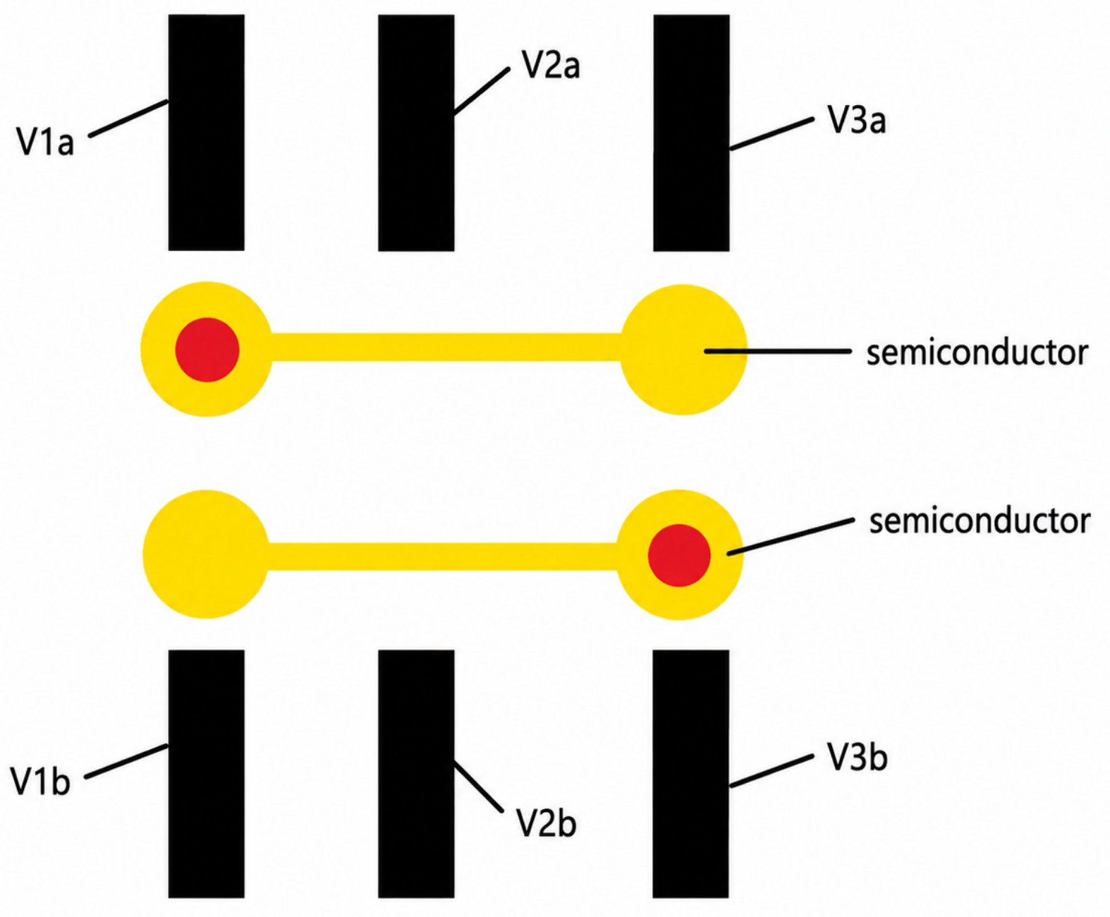
By proper numerical experiments one can establish proper and structure that maximizes the emission of entangled photons among all emitted photons that can be later translated into voltage signal pattern and with respect to the physical situation from Figure 13. The results obtained by the two-body Schrödinger formalism support the validity of the tight-binding model to a certain degree. More optimal two-entangled-photon emission as basing on structure depicted in Figure 12 can be optimized with reference to Figure 9, Figure 14, Figure 15, Figure 16, Figure 17, Figure 18 and Figure 19.
Figure 13.
Wavefunctions’ absolute value of interacting particles A and B placed at two different single-electron lines with an initial non-entangled state in the case of energy occupancy for each particle at time and after some time t. Oscillations are never fully periodic as the system heats up and each particle starts to occupy an increasing number of energy levels, which is directly the breakdown of the tight-binding model in longer time scales. One can refer to the next figure for more details.
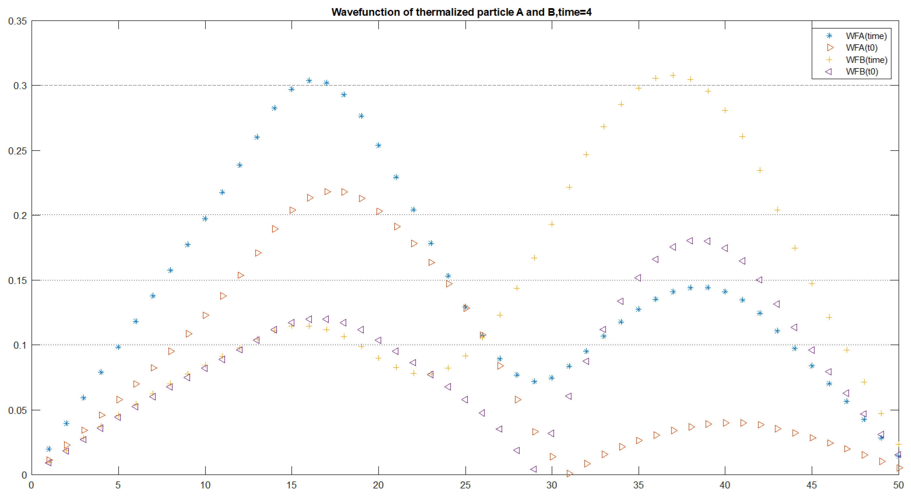
Figure 14.
Dependence of the quasi-classical SWAP-gate Hamiltonian on the electrostatically controlled polarizing potentials and , calculated for fixed values and .
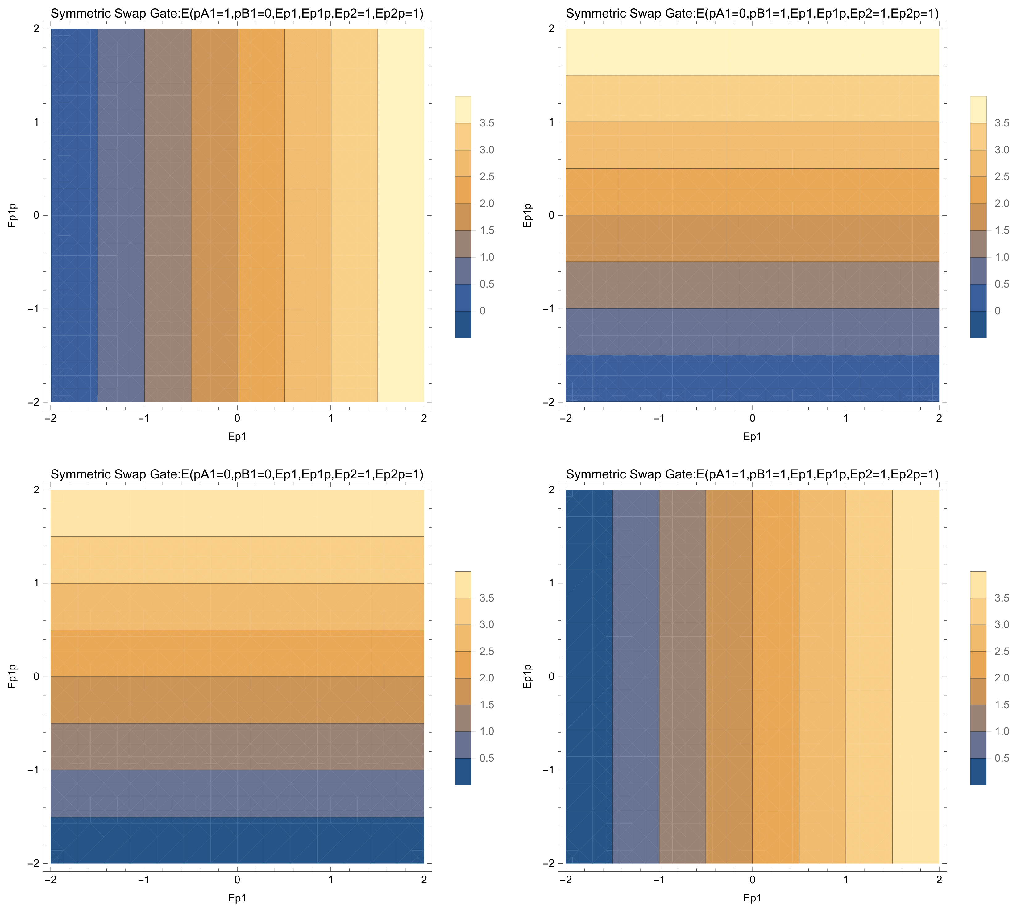
Figure 15.
Role of polarizing voltages in transition from symmetric classical and quantum SWAP gate in asymmetric SWAP gate (4 upper and bottom left) and in transition into ANTISWAP gate ((bottom right) plots).
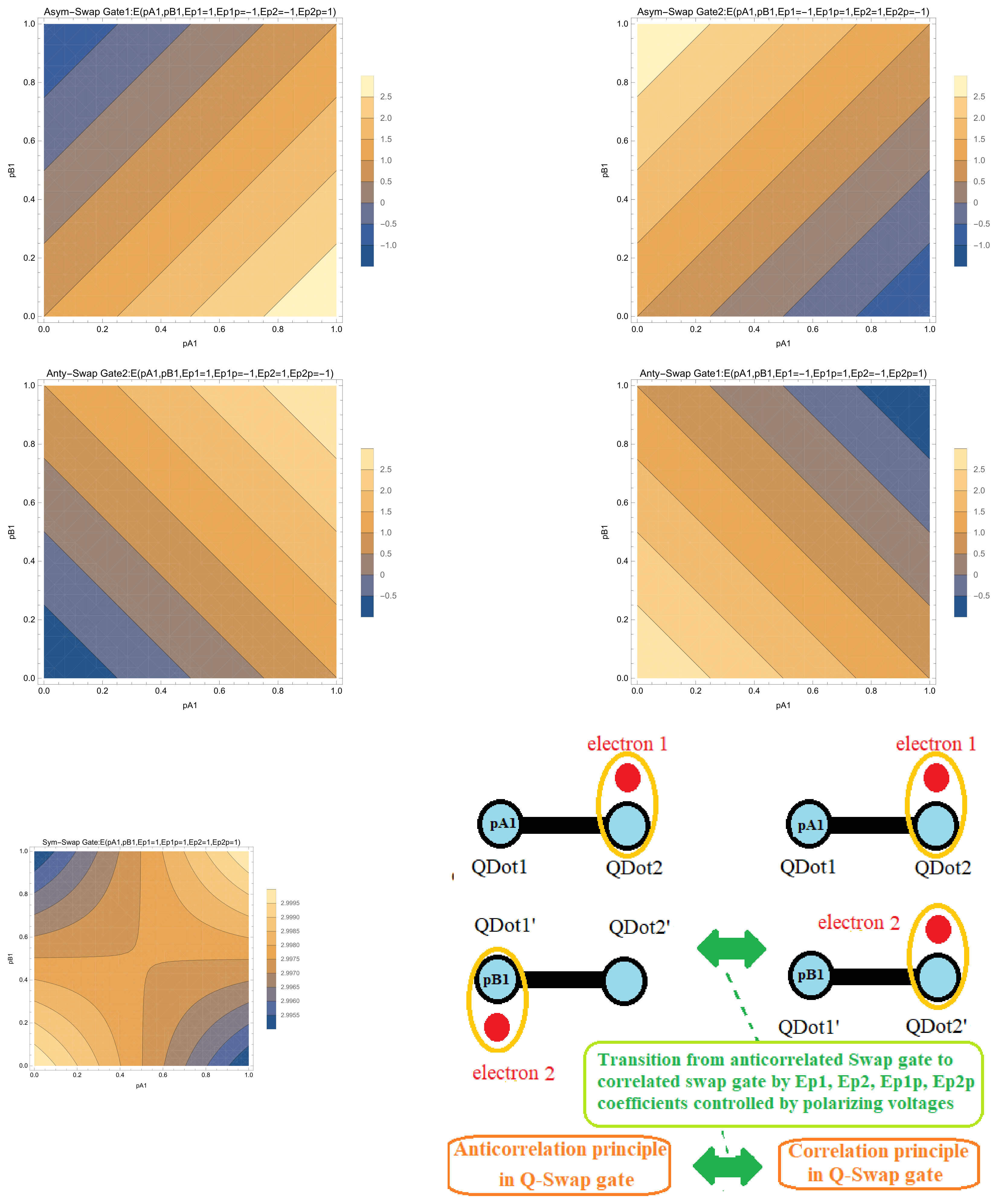
Figure 16.
Two main scenarios of dependence of eigenenergies of electrostatically interacting qubits on angles. The (left) plot corresponds to parameters (d = 1, a + b = 0.8, q = 1, , , , , , ), and the (right) plot has the same parameters except (, a + b = 0.1).
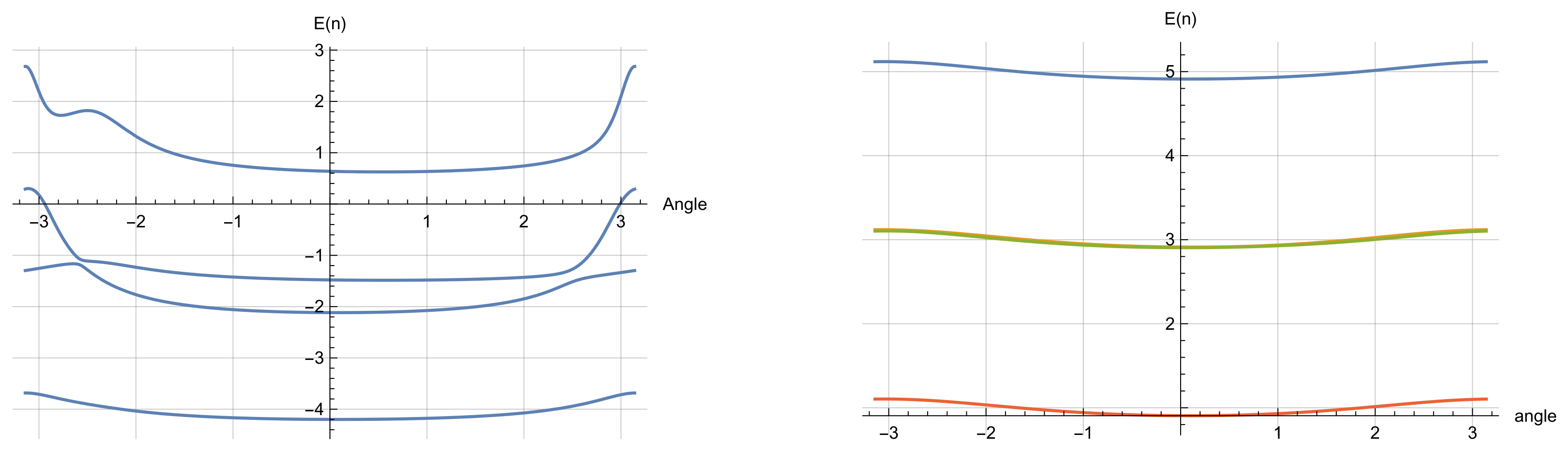
Figure 17.
Energy spectrum of generalized electrostatic quantum gate in dependence on angle for fixed , , , , , , . No crossing of energy levels was reported.
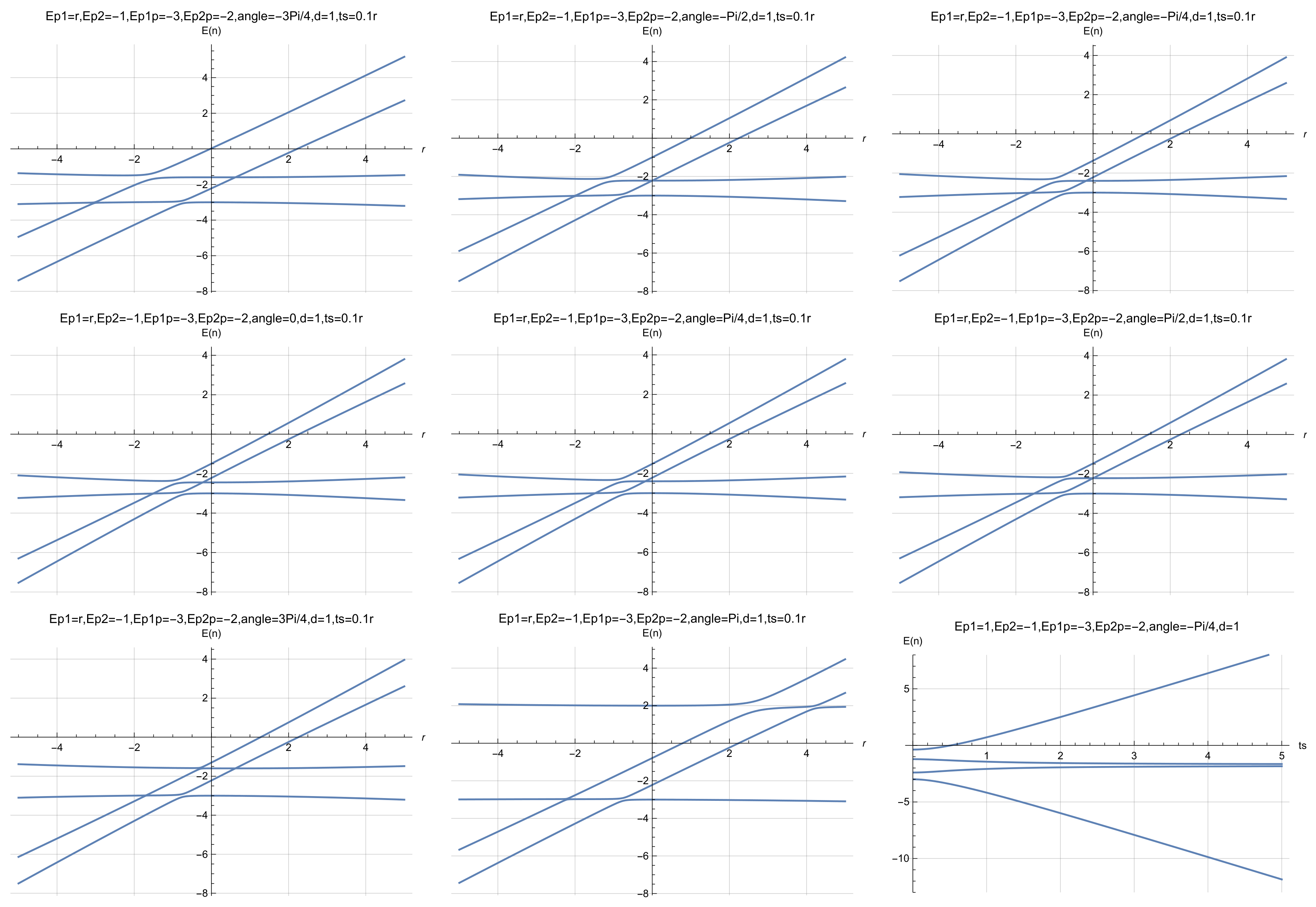
Figure 18.
Continuation of Figure 9: additional contour plots for the transition from the classical/quantum SWAP gate into the ANTISWAP gate as the angle is varied.
8.2. Case of Thermalization of Systems of Two Position-Based Qubits and Failure of Tight-Binding Model
We can set
which gives evolution of wavefunction modulus of each particle as in Figure 4 when the perturbative Coulomb interaction is turned on. It is interesting to observe how the non-entangled system is becoming more entangled with time as indicated by Figure 11. The dynamics of two electrons confined by two local potentials is determined for various cases both in analytical and in numerical way in the tight-binding model [44]. In this way, the system of two coupled electrostatic position-based qubits can be used for the implementation of the quantum SWAP or ANTISWAP gate. A broader picture is drawn by [29,44,45]. The obtained results have their meaning in designing the proper operation of the quantum gates implemented in chain of coupled semiconductor quantum dots that are electrostatically controlled. They open the path for implementation of a CMOS quantum computer that is only controlled by voltages applied to CMOS transistors with no need for usage of a magnetic field. It is an appealing alternative for the implementation of quantum electronics other than by the usage of Josephson junctions [9,46]. The best way of detecting the entanglement present between electrostatically interacting qubits is by experimentally measuring the correlation–anticorrelation function. Both formulas for von Neumann entanglement entropy and anticorrelation functions are given in this work in analytical form. In the next section we describe the elementary derivation of the tight-binding model from the Schrödinger formalism.
Figure 19.
Continuation of Figure 17: additional dependence of the same generalized electrostatic quantum-gate spectrum on the geometric and distance parameters.
9. Fundamental Derivation of the Tight-Binding Model from the Schrödinger Equation
After demonstrating both the usefulness and the limitations of the reduced model, this section returns to the microscopic Schrödinger equation to justify how the tight-binding parameters arise. Its purpose is to place the position-basis Hamiltonian on a more fundamental footing and to explain how the effective parameters should be interpreted when two separated qubits interact perturbatively. The derivation begins with a two-level energy-eigenstate description and constructs localized Wannier-like states through a basis rotation. Matrix elements of the kinetic-plus-potential Schrödinger operator are projected onto those localized states to obtain the effective on-site energies and tunneling amplitudes. For two interacting single-electron lines, Coulomb terms are added perturbatively and encoded through geometry-dependent coefficients. The manuscript then compares occupation dynamics obtained in the effective tight-binding model with the perturbative two-body Schrödinger evolution and discusses how the procedure can be generalized to more qubits provided that a restricted low-energy subspace remains meaningful.
The derivation clarifies that and are not fundamental constants of the device. They are matrix elements of a microscopic Hamiltonian evaluated in a chosen localized basis. Consequently, changes in confinement, electric field, interaction strength, or basis composition can change their effective values. This interpretation is consistent with the breakdown discussion of Section 8: when interactions populate states outside the original two-level subspace, a time-independent two-parameter description can no longer represent the full wavefunction. The section therefore connects the analytical convenience of tight binding with the microscopic conditions required for its validity.
Section 9 supplies the formal justification for the tight-binding Hamiltonian used throughout the manuscript and validates it as a projected low-energy model of the Schrödinger problem. It also explains why the effective parameters can become state- and time-dependent when the truncated basis is no longer closed. This provides the conceptual bridge between the compact gate model and the beyond-tight-binding conclusions of the work.
Being motivated by [45,46] and starting from the eigenenergy qubit as given by IBM Q-Experience and many other technologies () we arrive at
where we have since we assume . Here and account for the probability of occupancy of and energetic states. Maintenance of quantum information is about keeping it encoded in the Bloch sphere by two parameters (, ) and given in reference to quantum state by . Due to the compact size of the semiconductor quantum dots as depicted in Figure 3, it is vital to express the position-based qubit by stating its Hamiltonian in the so-called tight-binding model, where the quantum state is the linear superposition of two Wannier wavefunctions denoting maximal localization on the left or right quantum dot ():
where and are maximum localized Wannier wavefunctions (, ) on the left and right side respectively, while and give the probabilities for a particle (single electron or hole) to stay on the left and right quantum dots. Encoding quantum information by electron or hole position brings compactification of quantum chips. The quantum state in Wannier representation can be mapped to quantum state in energetic representation given as or reversely, and those two ways of description are fully equivalent.
Following [35,37] it is useful to introduce parameter
The precondition for occurrence of the position-based qubit is occupancy for at least two energetic levels, so neither nor is zero. Finally in the case of static Hamiltonian from Equation (83) also given by [37] the tight-binding Hamiltonian [35] appears as
We propose maximum localized orthonormal Wannier functions (so occupancy of is maximized from minus infinity to zero) of the form
Two Interacting Single-Electron Lines Described in the Tight-Binding Model and Validated by a Perturbative Schrödinger Model
We consider the system of two position-based qubits interacting perturbatively. Two electrons on two separated single-electron lines tend to be in anti-correlated positions due to repulsion force as depicted in Figure 3, Figure 6 and Figure 7. In such a way we encounter the situation of two electrons placed on two different left (right) quantum dots with probabilities () or the case left (right) occupancy of first dot and right (left) occupancy of second dot with probability () that specifies normalized quantum state () to be in the form as given by [37]:
In the case of two single-electron lines we can write the effective Hamiltonian to be of the form
Finally, we obtain validation of the tight-binding model in terms of the Schrödinger equation, so we end up with the following effective Hamiltonian.
where four terms are responsible for two qubits being at a distance d mutual Coulomb interaction (as depicted in Figure 3.) and given as
In the first approximation we consider two position-based qubits as non-interacting and slightly perturbed by the electrostatic single-electron to single-electron interaction, which naturally leads to first approximation of system eigenstate as the tensor product of two Hilbert spaces belonging to each qubits in the form as given below:
The search for the system ground state naturally implies minimization of Coulomb energy as a criterion for the lowest energy state that can be expressed by proper self-alignment of electrons in an anticorrelated way and thus leading to minimization of Coulomb interaction energy. Coulomb energy is given as
Coulomb energy minimization condition brings the following constrains
and hence we have
that leads to
Now we exercise the second constraint on energy minimization, which brings
and we obtain
Under the assumption that qubit A is occupying two energy levels and , while qubit B is occupying two energy levels and , we have
, , and . Geometry of the two electrostatically interacting structures is encoded in the , , and coefficients. We compute , ) in accordance with Formula (85) for qubits (A,B), and thus consequently we obtain the coefficients. By having values of … and consequently initial probability of occupancy eigenenergies in the case of separated but perturbatively interacting qubits and we can determine quantum dot occupancy during next time steps. Such a procedure can be attempted for N interacting qubits under condition of occupancy of two eigenenergy levels.
Qubits considered electrostatically interacting can be further subjected to Rabi oscillations by local microwave fields acting on qubits in their direct proximity, which might imply evolution of the system ground state with time.
It is quite straightforward to apply the presented scheme for the case of N position-based qubits implementing various quantum gates [36]. The obtained results have their significance in quantum communication as well [47].
10. Conclusions
The final section integrates the technological, analytical, and microscopic parts of the manuscript into a single assessment of the proposed electrostatic quantum-gate architecture. Its purpose is to identify what the model establishes, which remains conditional on the tight-binding approximation, and how the results can guide the design of CMOS-compatible single-electron quantum circuits. Across the work, a hierarchy of descriptions is used. The analysis begins with a two-state position qubit, extends it to a four-state Hamiltonian for two Coulomb-coupled double quantum dots, derives symmetric and asymmetric SWAP-related solutions, introduces quasiclassical energy landscapes for device tuning, maps between energy and position bases, and finally compares the reduced model with a perturbative two-body Schrödinger treatment. Gate behavior is characterized through charge-state probabilities, correlation/anticorrelation functions, and the von Neumann entropy. The device discussion connects these variables with electrostatic control, cryogenic CMOS compatibility, charge sensing, and numerical design workflows such as QTCAD [14,15].
The two QTCAD citations have distinct roles. Beaudoin et al. [14] used nonlinear Poisson–Schrödinger finite-element simulations with adaptive meshing to reproduce side-gate-activated corner-dot confinement in an industrial UTBB FD-SOI device and demonstrated robust solver convergence at 100 mK. Kriekouki et al. [15] then applied 3D quantum TCAD to a 28 nm FD-SOI device, comparing simulations with experiments to determine conditions for single-electron occupancy and Coulomb blockade. In the present article these works motivate the transition from compact analytical parameters to realistic device geometry; they are not used as evidence for the analytical derivations themselves.
The main result is that electrostatic two-qubit behavior can be organized around a small set of physically interpretable parameters: local confinement energies, tunnel couplings, Coulomb interaction energies, and geometry. Within the low-energy localized regime, these parameters provide analytical descriptions of SWAP, , ANTISWAP/repeater-like, correlated, and anticorrelated operating points. The quasiclassical treatment supplies intuitive energy-selection rules, whereas the fully quantum treatment shows how tunneling and coherent superposition convert electrostatic charge preferences into entanglement dynamics. The correlation/anticorrelation function and the von Neumann entropy provide complementary observables for following the transition from separable to entangled charge configurations.
A second major result is the explicit limitation of this picture. The perturbative Schrödinger analysis indicates that additional eigenstates can become populated with time, so the original two-level-per-qubit basis does not remain closed indefinitely. In this regime, the effective on-site energies and hopping amplitudes should be understood as low-energy matrix elements whose apparent time dependence can signal the influence of neglected states. The observation does not remove the usefulness of tight binding; rather, it defines the regime in which the compact analytical formulas can be used reliably and indicates when a larger Hilbert space, self-consistent Schrödinger–Poisson treatment, Hubbard-type extension, or another beyond-tight-binding method is required. The discussion of photonic tight-binding analogies [48] further emphasizes that similar mathematics can appear in different physical platforms while the underlying particle statistics and interaction mechanisms remain different.
Taken together, the manuscript provides a coherent analytical framework for voltage-controlled quantum logic in coupled semiconductor quantum dots. Its strongest contribution is the connection between device geometry, electrostatic bias, tunneling, charge correlation, and entanglement within a CMOS-oriented position-basis architecture. The derived formulas provide design rules for tuning correlated and anticorrelated operating regimes and identify charge observables that can be related to experimental readout. At the same time, the work demonstrates that the tight-binding approximation has a finite domain of validity: longer-time evolution, higher-state occupation, stronger driving, and many-body effects require a broader microscopic treatment. The proposed architecture is therefore best interpreted as a scalable low-energy gate framework that can serve as the analytical core of more complete numerical design tools, while experiments must determine the parameter window in which the two-level-per-qubit approximation remains quantitatively accurate. Preliminary examples of computer code incorporating tight-binding model and mathematical formulas for noise model in tight-binding model approach to single-electron semiconductor devices are included in Appendix A and Appendix B. Topological phase transitions as given by [49,50,51] can take place in superconducting-single electron semiconductor devices interfaced to Josephson junction can be grasped by tight-binding model [23]. Various experiments on single-electrons in nanostructures as given by [52,53,54,55,56,57] can be described by tight-binding model.
Author Contributions
Conceptualization, K.P.; Methodology, K.P.; Software, K.P., E.H. and A.M.; Validation, K.P. and A.M.; Formal analysis, K.P.; Investigation, K.P.; Writing—original draft, K.P.; Writing—review & editing, K.P., E.H. and A.M.; Visualization, E.H.; Supervision, K.P. All authors have read and agreed to the published version of the manuscript.
Funding
Partial support was obtained from grant NQVL:QSTD:Pilot: Quantum Computing Applications of Photonics (QCAP) with Award Abstract: 2410813.
Data Availability Statement
The original contributions presented in this study are included in the article. Further inquiries can be directed to the corresponding author.
Acknowledgments
We acknowledge partial financial support from Quantum Hardware Systems from Lodz in Poland and from Quantum Hardware Software Systems LLC company in Albuquerque in USA. We also thank Erik Staszewski (University College Dublin) for assistance with figure preparation. Special acknowledgment is expressed to Practical Electronics and Microelectronics Scientific Student Association (PEMSSA) and Schroedinger’s Cat at Lodz University of Technology, where many ideas were discussed and shaped.
Conflicts of Interest
Dr. Krzysztof Pomorski is founder and Eryk Halubek is consultant and scientific collaborator of Quantum Hardware Software Systems LLC, based in Albuquerque, New Mexico, USA. Dr. Krzysztof Pomorski serves as Chief Executive Officer (CEO), and Artur Michalak serves as Chief Operating Officer (COO) of Quantum Hardware Systems, based in Poland. The authors declare that the research was conducted in the absence of any commercial or financial relationships that could be construed as a potential conflict of interest.
Appendix A. Explicit Simulation Codes in Wolfram Mathematica Software
The system of two interacting position-based qubits in the tight-binding model can be characterized by four energy eigenvalues encoded in Mathematica Wolfram by a chain of commands
E1qq[Ep1A_, Ep2A_, Ep1B_, Ep2B_, d_, a_, b_, tsA_, tsB_, ThetaA_, ThetaB_, q_] :=
Eigenvalues[{{Ep1A + Ep1B + (q^2/d), tsB Exp[Sqrt[−1] ThetaB],
tsA Exp[Sqrt[−1] ThetaA], 0}, {tsB Exp[−Sqrt[−1] ThetaB],
Ep1A + Ep2B + (q^2/Sqrt[d^2 + (a + b)^2]), 0,
tsA Exp[Sqrt[−1] ThetaA]}, {tsA Exp[−Sqrt[−1] ThetaA], 0,
Ep2A + Ep1B + (q^2/Sqrt[d^2 + (a + b)^2]),
tsB Exp[Sqrt[−1] ThetaB]}, {0, tsA Exp[−Sqrt[−1] ThetaA],
tsB Exp[−Sqrt[−1] ThetaB], Ep2A + Ep2B + (q^2/d)}}][[1]]
E2qq[Ep1A_, Ep2A_, Ep1B_, Ep2B_, d_, a_, b_, tsA_, tsB_, ThetaA_, ThetaB_, q_] :=
Eigenvalues[{{Ep1A + Ep1B + (q^2/d), tsB Exp[Sqrt[−1] ThetaB],
tsA Exp[Sqrt[−1] ThetaA], 0}, {tsB Exp[−Sqrt[−1] ThetaB],
Ep1A + Ep2B + (q^2/Sqrt[d^2 + (a + b)^2]), 0,
tsA Exp[Sqrt[−1] ThetaA]}, {tsA Exp[−Sqrt[−1] ThetaA], 0,
Ep2A + Ep1B + (q^2/Sqrt[d^2 + (a + b)^2]),
tsB Exp[Sqrt[−1] ThetaB]}, {0, tsA Exp[−Sqrt[−1] ThetaA],
tsB Exp[−Sqrt[−1] ThetaB], Ep2A + Ep2B + (q^2/d)}}][[2]]
E3qq[Ep1A_, Ep2A_, Ep1B_, Ep2B_, d_, a_, b_, tsA_, tsB_, ThetaA_, ThetaB_, q_] :=
Eigenvalues[{{Ep1A + Ep1B + (q^2/d), tsB Exp[Sqrt[−1] ThetaB],
tsA Exp[Sqrt[−1] ThetaA], 0}, {tsB Exp[−Sqrt[−1] ThetaB],
Ep1A + Ep2B + (q^2/Sqrt[d^2 + (a + b)^2]), 0,
tsA Exp[Sqrt[−1] ThetaA]}, {tsA Exp[−Sqrt[−1] ThetaA], 0,
Ep2A + Ep1B + (q^2/Sqrt[d^2 + (a + b)^2]),
tsB Exp[Sqrt[−1] ThetaB]}, {0, tsA Exp[−Sqrt[−1] ThetaA],
tsB Exp[−Sqrt[−1] ThetaB], Ep2A + Ep2B + (q^2/d)}}][[3]]
E4qq[Ep1A_, Ep2A_, Ep1B_, Ep2B_, d_, a_, b_, tsA_, tsB_, ThetaA_, ThetaB_, q_] :=
Eigenvalues[{{Ep1A + Ep1B + (q^2/d), tsB Exp[Sqrt[−1] ThetaB],
tsA Exp[Sqrt[−1] ThetaA], 0}, {tsB Exp[−Sqrt[−1] ThetaB],
Ep1A + Ep2B + (q^2/Sqrt[d^2 + (a + b)^2]), 0,
tsA Exp[Sqrt[−1] ThetaA]}, {tsA Exp[−Sqrt[−1] ThetaA], 0,
Ep2A + Ep1B + (q^2/Sqrt[d^2 + (a + b)^2]),
tsB Exp[Sqrt[−1] ThetaB]}, {0, tsA Exp[−Sqrt[−1] ThetaA],
tsB Exp[−Sqrt[−1] ThetaB], Ep2A + Ep2B + (q^2/d)}}][[4]]
Plot[{E1qq[1, 1, 1, 1, d, 0.1, 0.1, 1, 1, 0, 0, 1],
E2qq[1, 1, 1, 1, d, 0.1, 0.1, 1, 1, 0, 0, 1],
E3qq[1, 1, 1, 1, d, 0.1, 0.1, 1, 1, 0, 0, 1],
E4qq[1, 1, 1, 1, d, 0.1, 0.1, 1, 1, 0, 0, 1]}, {d, 0.1, 1}]
-
that correspond to the following dependence of eigenenergies on distances as given by Figure A1. It should be noticed that ground kinetic energy for the electron confined in Si across the region of L = 5 nm is meV, while electron–electron electrostatic energy at a distance of d = 5 nm results in a value in range of meV. Therefore localized energy in the tight-binding model at nodes 1 and 2 given as , and hopping terms are in that value range.
Figure A1.
Case of dependence of different energy eigenvalues vs. distance for 2 electrostatically interacting single-electron position-based qubits.
Appendix B. Impact of Noise on Tight-Binding Model Parameters
Let us consider the effective potential for one position-based qubits being given by with the condition that and the corresponding set of self-control functions for time-dependent fluctuating potential and non-fluctuating . Based on Formula (85)
where no Rabi oscillations were assumed due to the low frequency of the fluctuating effective potential component with a constant with time effective potential component . More sophisticated noise models are given in [58]. One shall also be aware of limitations of electrostatic single-electron devices as given by [52].
Appendix C. Qubit–Qubit Interaction with Two Symmetric Conditions
Appendix C.1. Case I: Ef (1, 1′) = Ef (1, 2′) = U, Ef (2, 1′) = Ef (2, 2′) = U1
We postulate
We obtain
and it implies
We also have
and we obtain
that implies condition
that is fulfilled for two angles as in accordance to numerical solutions. Usually since in most cases qubit size is small in comparison to the distance between qubits. Let us solve the problem with certain approximation by using Taylor expansion
It implies
and hence we have
Using Taylor expansion for the square root function we obtain relation
that can be simplified into simple relation for the sinusoidal function of the form
Two angles fulfill such a relation.
We can also solve Equation (A7) in a rigorous way (without approximation) equivalent to the following relation
and this implies
and finally we have
We obtain
This implies
We recognize that we have three free parameters that predetermine given as
Using three free parameters we obtain
We have four energy eigenvalues
and we obtain the following eigenstates
Appendix C.2. Case II: Ef (1, 1′) = Ef (2, 2′) = U, Ef (1, 2′) = Ef (2, 1′) = U1
We postulate
that implies
and consequently we obtain
We also have
and it implies
This results in
and
Therefore we have three open parameters , , and for any we have predetermined conditions for and given as
and
and implies
as well as
We have the following eigenvalues
and eigenstates
Appendix C.3. Case III: Ef (1, 1′) = Ef (2, 1′) = U, Ef (1, 2′) = Ef (2, 2′) = U1
We postulate
that implies , and we obtain
We also have
which implies
and consequently we obtain the condition
that is fulfilled for one angle . It gives us three controlling parameters , , for given that determine
We obtain the following Hamiltonian eigenvalues and eigenstates
and
Appendix C.4. Case of Density Matrix in the Case of Two Interacting Particles in the Symmetric Case
We consider the simplifying matrix and highly symmetric matrix of the form
that has only real-valued components with , and , , , . We obtain the density matrix
with the following components of unitary matrix
We set the quantum state to be at time so it is maximally entangled and its density matrix is . Finally we obtain the following density matrix
It transpires that , so one deals with a pure quantum state. Now we are obtaining reduced matrices describing the state of particle B from a two-particle density matrix.
Consequently we can compute entanglement entropy. At first we evaluate
Appendix D. Analytical Treatment of Two Interacting Particles in Asymmetric Case
We consider the situation as depicted in Figure 6. We obtain the following Hamiltonian
In a general situation all eigenvalues and eigenstates of this matrix can be determined in an analytical way since roots of fourth-order polynomials are given by explicit formulas. However those formulas are very complicated and thus not so practical. We will make radical simplifications leading to simple formulas for quantum eigenstates and eigenenergies. The first main assumption is setting . We obtain a simplified Hamiltonian of the form
More detailed cases are given in the appendix in the section “Qubit–Qubit Interaction With Two Symmetric Conditions”.
Appendix D.1. Correlation Function for Case II: Ef (1, 1′) = Ef (2, 1′) = U, Ef (1, 2′) = Ef (2, 2′) = U1
We postulate
that implies
and consequently we obtain
We also have
and it implies
This results in
and
Therefore we have three open parameters , , and for any we have predetermined conditions for and given as
and
and implies
as well as
We have the following eigenvalues
and eigenstates
Appendix D.2. Correlation Function for Case III: Ef (1, 1′) = Ef (2, 1′) = U
Now we generalize the Hamiltonian matrix of the form
and energy eigenvalues dependent on , , U and are given as
It is surprising to discover that the corresponding energy eigenstates are dependent only on the hopping constant and are not dependent on the hopping constant and are given as
The minimalist density matrix of two electrostatically interacting qubits A and B in the tight-binding model in the case of the time-independent Hamiltonian is given as
where , , and are probabilities of occupancy of eigenenergies , , and and we obtain two-particle density-matrix diagonal elements in the detailed form given below. We have the probability of finding electron A at node 1 and electron B at node 1’ given by formula
and the probability of finding electron A at node 1 and electron B at node 2’ given by formula
and the probability of finding electron A at node 2 and electron B at node 1′ given as
and the probability of finding electron A at node 2 and electron B at node 2′ as
Appendix E. Analytical Method for Prediction of Correlation–Anticorrelation in Generalized SWAP Gate
We can predict correlation or anticorrelation by monitoring the sign of the correlation function with correlation function operator C
and under the circumstances of the time-independent Hamiltonian we have
When has negative values the SWAP gate is employed, while the ANTISWAP gate requires a positive value.
Correlation Function for Case I: Ef (1,1′) = Ef (1,2′) = U, Ef (2,1′) = Ef (2,2′) = U1
For the qubit–qubit Hamiltonian of structure
we obtain the following correlation function
where , , , are probabilities for the system of coupled qubits to occupy energy level , , , , and the normalization condition is fulfilled . We encounter a mixture of time-dependent cos or sin oscillations of different frequencies as , , , , , where the quantum state is given as
Here we have tuning coefficients , , , , . The probability of occupancy of is of the following form
and
The density matrix of two interacting particles allows us to obtain density matrices of particles A and B. The elements of density matrix A are given as
We also obtain the density matrix of particle B (electron at nodes 1′ and 2′) in the form of
It remarkable to notice that the hopping constant that was constant for position-dependent qubit was modified, and it has two parts that depends on the frequency and For given density matrix
where , , , in R with we identify von Neumann entanglement S entropy expressed as
References
- Fujisawa, T.; Oosterkamp, T.H.; van der Wiel, W.G.; Broer, B.W.; Aguado, R.; Tarucha, S.; Kouwenhoven, L.P. Spontaneous Emission of Phonons in a Semiconductor Quantum Dot. Science 1998, 282, 932–935. [Google Scholar] [CrossRef] [Scilit] [PubMed]
- Likharev, K.K. Single-electron devices and their applications. Proc. IEEE 1999, 87, 606–632. [Google Scholar] [CrossRef] [Scilit]
- Fujisawa, T.; Hirayama, Y. Transmission Type RF Single Electron Transistor Operation of a Semiconductor Quantum Dot. Jpn. J. Appl. Phys. 2000, 39, 2338. [Google Scholar] [CrossRef] [Scilit]
- Veldhorst, M.; Yang, C.H.; Hwang, J.; Huang, W.; Dehollain, J.P.; Muhonen, J.T.; Simmons, S.; Laucht, A.; Hudson, F.E.; Itoh, K.M.; et al. A two-qubit logic gate in silicon. Nature 2015, 526, 410–414. [Google Scholar] [CrossRef] [Scilit] [PubMed]
- Pekola, J.P.; Saira, O.-P.; Maisi, V.F.; Kemppinen, A.; Möttönen, M.; Pashkin, A.Y.; Averin, D.V. Single-electron current sources: Toward a refined definition of the ampere. Rev. Mod. Phys. 2013, 85, 1421. [Google Scholar] [CrossRef] [Scilit]
- Weis, J. Single-Electron Devices. In CFN Lectures on Functional Nanostructures; Volume 1, Lecture Notes in Physics & Volume 658; Springer: Berlin/Heidelberg, Germany, 2004. [Google Scholar] [CrossRef] [Scilit]
- Gustavsson, S.; Leturcq, R.; Simovic, B.; Schleser, R.; Ihn, T.; Studerus, P.; Ensslin, K.; Driscoll, D.C.; Gossard, A.C. Counting Statistics of Single Electron Transport in a Quantum Dot. Phys. Rev. Lett. 2006, 96, 076605. [Google Scholar] [CrossRef] [Scilit] [PubMed]
- Wang, K.; Payette, C.; Dovzhenko, Y.; Deelman, P.W.; Petta, J.R. Charge Relaxation in a Single-Electron Si/SiGe Double Quantum Dot. Phys. Rev. Lett. 2013, 111, 046801. [Google Scholar] [CrossRef] [Scilit] [PubMed]
- Stehlik, J.; Dovzhenko, Y.; Petta, J.R.; Johansson, J.R.; Nori, F.; Lu, H.; Gossard, A.C. Landau–Zener–Stuckelberg Interferometry of a Single Electron Charge Qubit. Phys. Rev. B 2012, 86, 121303. [Google Scholar] [CrossRef] [Scilit]
- Durrani, Z.A.K. Coulomb Blockade, Single-Electron Transistors and Circuits in Silicon. Phys. E 2003, 17, 572–578. [Google Scholar] [CrossRef] [Scilit]
- Korotkov, A.N. Coulomb Blockade and Digital Single-Electron Devices. In Molecular Electronics; Jortner, J., Ratner, M.A., Eds.; Blackwell Science: Oxford, UK, 1997; pp. 157–189. [Google Scholar]
- Gonzalez-Zalba, M.F.; Shevchenko, S.N.; Barraud, S.; Johansson, J.R.; Ferguson, A.J.; Nori, F.; Betz, A.C. Gate-Sensing Coherent Charge Oscillations in a Silicon Field-Effect Transistor. Nano Lett. 2016, 16, 1614–1619. [Google Scholar] [CrossRef] [Scilit] [PubMed]
- Schaal, S.; Barraud, S.; Morton, J.J.L.; Gonzalez-Zalba, M.F. Conditional Dispersive Readout of a CMOS Single-Electron Memory Cell. Phys. Rev. Appl. 2018, 9, 054016. [Google Scholar] [CrossRef] [Scilit]
- Beaudoin, F.; Philippopoulos, P.; Zhou, C.; Kriekouki, I.; Pioro-Ladriere, M.; Guo, H.; Galy, P. Robust Technology Computer-Aided Design of Gated Quantum Dots at Cryogenic Temperature. Appl. Phys. Lett. 2022, 120, 264001. [Google Scholar] [CrossRef] [Scilit]
- Kriekouki, I.; Beaudoin, F.; Philippopoulos, P.; Zhou, C.; Lemyre, J.C.; Rochette, S.; Rohrbacher, C.; Mir, S.; Barragan, M.J.; Pioro-Ladriere, M.; et al. Understanding Conditions for the Single Electron Regime in 28 nm FD-SOI Quantum Dots: Interpretation of Experimental Data with 3D Quantum TCAD Simulations. Solid-State Electron. 2023, 204, 108626. [Google Scholar] [CrossRef] [Scilit]
- Zwanenburg, F.A.; Dzurak, A.S.; Morello, A.; Simmons, M.Y.; Hollenberg, L.C.L.; Klimeck, G.; Rogge, S.; Coppersmith, S.N.; Eriksson, M.A. Silicon quantum electronics. Rev. Mod. Phys. 2013, 85, 961–1019. [Google Scholar] [CrossRef] [Scilit]
- Chatterjee, A.; Stevenson, P.; Franceschi, S.D.; Morello, A.; de Leon, N.P.; Kuemmeth, F. Semiconductor qubits in practice. Nat. Rev. Phys. 2021, 3, 157–177. [Google Scholar] [CrossRef] [Scilit]
- Krantz, P.; Kjaergaard, M.; Yan, F.; Orlando, T.P.; Gustavsson, S.; Oliver, W.D. A quantum engineer’s guide to superconducting qubits. Appl. Phys. Rev. 2019, 6, 021318. [Google Scholar] [CrossRef] [Scilit]
- Petit, L.; Eenink, H.G.J.; Russ, M.; Lawrie, W.I.L.; Hendrickx, N.W.; Philips, S.G.J.; Clarke, J.S.; Vandersypen, L.M.K.; Veldhorst, M. Universal quantum logic in hot silicon qubits. arXiv 2019, arXiv:1910.05289. [Google Scholar]
- Stano, P.; Loss, D. Review of performance metrics of spin qubits in gated semiconducting nanostructures. Nat. Rev. Phys. 2022, 4, 672–688. [Google Scholar] [CrossRef] [Scilit]
- Loss, D.; DiVincenzo, D.P. Quantum computation with quantum dots. Phys. Rev. A 1998, 57, 120–126. [Google Scholar] [CrossRef] [Scilit]
- Burkard, G.; Ladd, T.D.; Pan, A.; Nichol, J.M.; Petta, J.R. Semiconductor spin qubits. Rev. Mod. Phys. 2023, 95, 025003. [Google Scholar] [CrossRef] [Scilit]
- Pomorski, K.D.; Peczkowski, P.; Staszewski, R.B. Analytical solutions for N interacting electron system confined in graph of coupled electrostatic semiconductor and superconducting quantum dots in tight-binding model. Cryogenics 2020, 109, 103117. [Google Scholar] [CrossRef] [Scilit]
- Hubbard, J. Electron correlations in narrow energy bands. Proc. R. Soc. Lond. A. Math. Phys. Sci. 1963, 276, 238–257. [Google Scholar] [CrossRef] [Scilit]
- Anderson, P.W. Absence of Diffusion in Certain Random Lattices. Phys. Rev. 1958, 109, 1492–1505. [Google Scholar] [CrossRef] [Scilit]
- Imada, M.; Fujimori, A.; Tokura, Y. Metal-insulator transitions. Rev. Mod. Phys. 1998, 70, 1039. [Google Scholar] [CrossRef] [Scilit]
- Spalek, J. Wstep Do Fizyki Materii Skondensowanej; PWN-Polish Scientific Publishers: Warsaw, Poland, 2015. [Google Scholar]
- Xu, H.Q. Method of calculations for electron transport in multiterminal quantum systems based on real-space lattice models. Phys. Rev. B 2002, 66, 165305. [Google Scholar] [CrossRef] [Scilit]
- Fujisawa, T.; Hayashi, T.; Cheong, H.D.; Jeong, Y.H.; Hirayama, Y. Rotation and phase-shift operations for a charge qubit in a double quantum dot. Phys. E 2004, 21, 1046–1052. [Google Scholar] [CrossRef] [Scilit]
- Petersson, K.D.; Petta, J.R.; Lu, H.; Gossard, A.C. Quantum coherence in a one-electron semiconductor charge qubit. Phys. Rev. Lett. 2010, 105, 246804. [Google Scholar] [CrossRef] [Scilit] [PubMed]
- Leipold, D. Controlled Rabi Oscillations as Foundation for Entangled Quantum Aperture Logic; Seminar, UC Berkeley Quantum Labs: Berkeley, CA, USA, 2018. [Google Scholar]
- Pomorski, K.; Giounanlis, P.; Blokhina, E.; Leipold, D.; Peczkowski, P.; Staszewski, R.B. From two types of electrostatic position dependent semiconductor qubits to quantum universal gates and hybrid semiconductor–superconducting quantum computer. In Superconductivity and Particle Accelerators; SPIE: 11054, Superconductivity and Particle Accelerators 2018; 110540M; SPIE Digital Library: Bellingham, WA, USA, 2018. [Google Scholar]
- Pomorski, K.; Giounanlis, P.; Blokhina, E.; Leipold, D.; Staszewski, R.B. Analytic view on coupled single-electron lines. Semicond. Sci. Technol. 2019, 34, 125015. [Google Scholar] [CrossRef] [Scilit]
- Baez, J.C.; Pollard, B.S. Quantropy. Entropy 2015, 17, 772–789. [Google Scholar] [CrossRef] [Scilit]
- Pomorski, K. Equivalence between finite state stochastic machine, non-dissipative and dissipative tight-binding and Schroedinger model. Math. Comput. Simulation 2023, 209, 362–407. [Google Scholar] [CrossRef] [Scilit]
- Pomorski, K. Analytic view on N body interaction in electrostatic quantum gates and decoherence effects in tight-binding model. Int. J. Quantum Inf. 2021, 19, 2141001. [Google Scholar] [CrossRef] [Scilit]
- Pomorski, K. Electrostatically Interacting Wannier Qubits in Curved Space. Materials 2024, 17, 4846. [Google Scholar] [CrossRef] [Scilit] [PubMed]
- Pomorski, K.; Nowakowski, W.; Michalak, A. Poster on Integrated Quantum Photonic Neural Networks Iinterfaced with Quantum Computers. APS March Meeting 2026. Available online: https://meetings-archive.aps.org/smt/2026/apr-l87/4/ (accessed on 9 February 2015).
- Kang, H.H.; Rosen, T.I.; Hays, M.; Grover, A.J.; Oliver, D.W. Remote entangling gates for spin qubits in quantum dots using a charge-sensitive superconducting coupler. Phys. Rev. Appl. 2025, 23, 044055. [Google Scholar] [CrossRef] [Scilit]
- Borjans, F.; Croot, X.G.; Mi, X.; Gullans, M.J.; Petta, J.R. Resonant microwave-mediated interactions between distant electron spins. Nature 2020, 577, 195–198. [Google Scholar] [CrossRef] [Scilit] [PubMed]
- Park, K.T.; Kim, K.H.; Min, B.J.; No, Y.S. Normal mode analysis in multi-coupled non-Hermitian optical nanocavities. Sci. Rep. 2023, 13, 17510. [Google Scholar] [CrossRef] [Scilit] [PubMed]
- Jaynes, E.T.; Cummings, F.W. Comparison of quantum and semiclassical radiation theories with application to the beam maser. Proc. IEEE 1963, 51, 89–109. [Google Scholar] [CrossRef] [Scilit]
- Fulton, T.A.; Dolan, G.J. Observation of single-electron charging effects in small tunnel junctions. Phys. Rev. Lett. 1987, 59, 109. [Google Scholar] [CrossRef] [Scilit] [PubMed]
- Zwerver, A.M.J.; Krähenmann, T.; Watson, T.F.; Lampert, L.; George, H.C.; Pillarisetty, R.; Bojarski, S.A.; Amin, P.; Amitonov, S.V.; Boter, J.M.; et al. Qubits made by advanced semiconductor manufacturing. Nat. Electron. 2022, 5, 184–190. [Google Scholar] [CrossRef] [Scilit]
- Fujisawa, T.; Hayashi, T.; Hirayama, Y.; Cheong, H.D.; Jeong, Y.H. Electron counting of single-electron tunneling current. Appl. Phys. Lett. 2004, 84, 2343–2345. [Google Scholar] [CrossRef] [Scilit]
- Mills, A.R.; Zajac, D.M.; Gullans, M.J.; Schupp, F.J.; Hazard, T.M.; Petta, J.R. Shuttling a single charge across a one-dimensional array of silicon quantum dots. Nat. Commun. 2019, 10, 1063. [Google Scholar] [CrossRef] [Scilit] [PubMed]
- Pomorski, K.; Staszewski, R.B. Towards quantum internet and non-local communication in position-based qubits. AIP Conf. Proc. 2020, 2241, 020030. [Google Scholar] [CrossRef] [Scilit]
- Laba, H.P.; Tkachuk, V.M. Quantum-mechanical analogy and supersymmetry of electromagnetic wave modes in planar waveguides. Phys. Rev. A 2014, 89, 033826. [Google Scholar] [CrossRef] [Scilit]
- Choi, M.S.; Yi, J.; Choi, M.Y.; Choi, J.; Lee, S.I. Quantum phase transitions in Josephson-junction chains. Phys. Rev. B 1998, 57, R716–R719. [Google Scholar] [CrossRef] [Scilit][Green Version]
- Sachdev, S. Quantum Phase Transitions, 2nd ed.; Cambridge University Press: Cambridge, UK, 2011. [Google Scholar]
- Maile, D.; Andergassen, S.; Belzig, W. Quantum phase transition with dissipative frustration. Phys. Rev. B 2018, 97, 155427. [Google Scholar] [CrossRef] [Scilit]
- Weichselbaum, A.; Ulloa, S.E. Charge qubits and limitations of electrostatic quantum gates. Phys. Rev. A 2004, 70, 032328. [Google Scholar] [CrossRef] [Scilit]
- Hayashi, T.; Fujisawa, T.; Cheong, H.D.; Jeong, Y.H.; Hirayama, Y. Coherent Manipulation of Electronic States in a Double Quantum Dot. Phys. Rev. Lett. 2003, 91, 226804. [Google Scholar] [CrossRef] [Scilit] [PubMed]
- Wingreen, N.S. Quantum Many-Body Effects in a Single-Electron Transistor. Science 2004, 304, 1258–1259. [Google Scholar] [CrossRef] [Scilit] [PubMed]
- Gorman, J.; Hasko, D.G.; Williams, D.A. Charge-Qubit Operation of an Isolated Double Quantum Dot. Phys. Rev. Lett. 2005, 95, 090502. [Google Scholar] [CrossRef] [Scilit] [PubMed]
- Fujisawa, T.; Hayashi, T.; Sasaki, S. Time-dependent single-electron transport through quantum dots. Rep. Prog. Phys. 2006, 69, 759–796. [Google Scholar] [CrossRef] [Scilit]
- Fujisawa, T.; Shinkai, G.; Hayashi, T.; Ota, T. Multiple two-qubit operations for a coupled semiconductor charge qubit. Phys. E Low-Dimens. Syst. Nanostructures 2011, 43, 730–734. [Google Scholar] [CrossRef] [Scilit]
- Yang, Y.C.; Coppersmith, S.N.; Friesen, M. Achieving high-fidelity single-qubit gates in a strongly driven charge qubit with 1/f charge noise. npj Quantum Inf. 2019, 5, 12. [Google Scholar] [CrossRef] [Scilit]
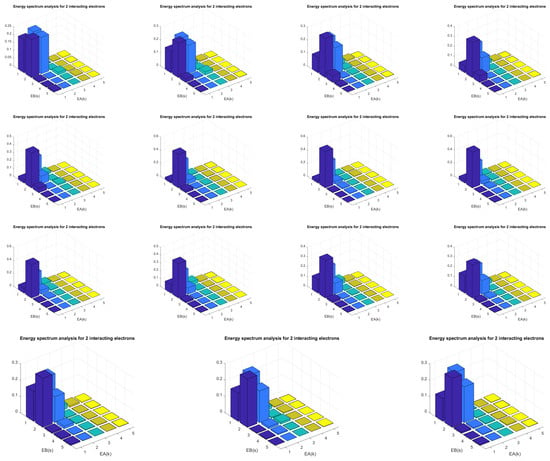
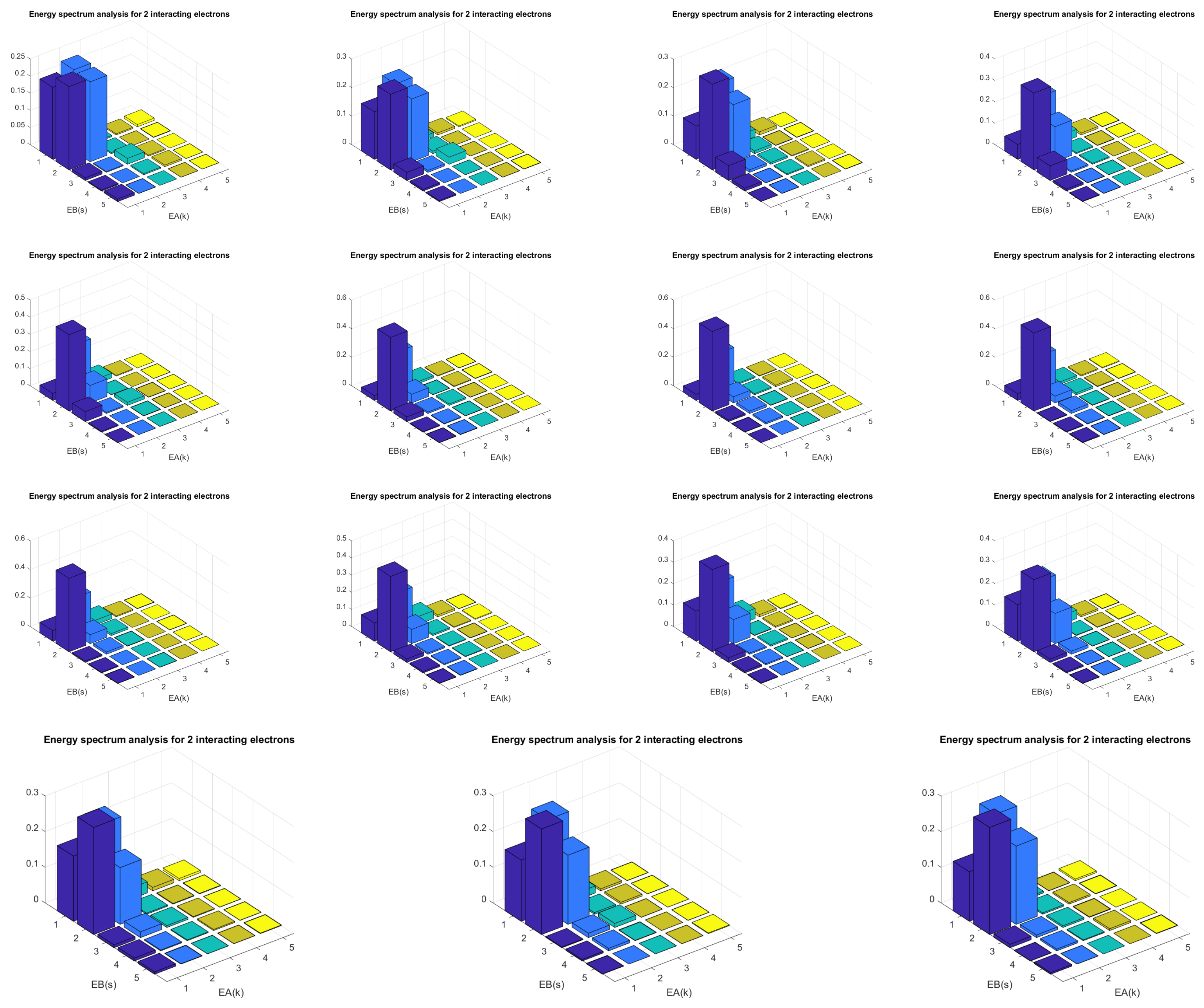
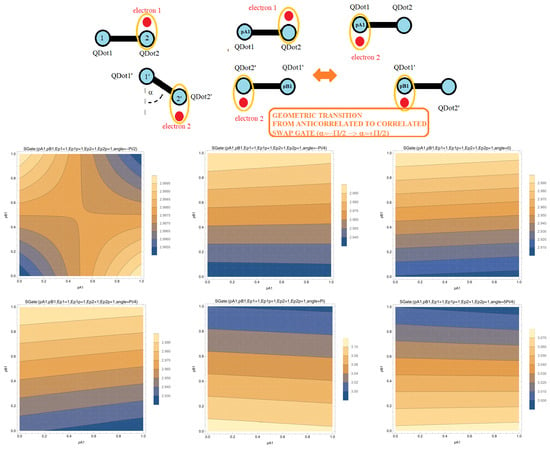
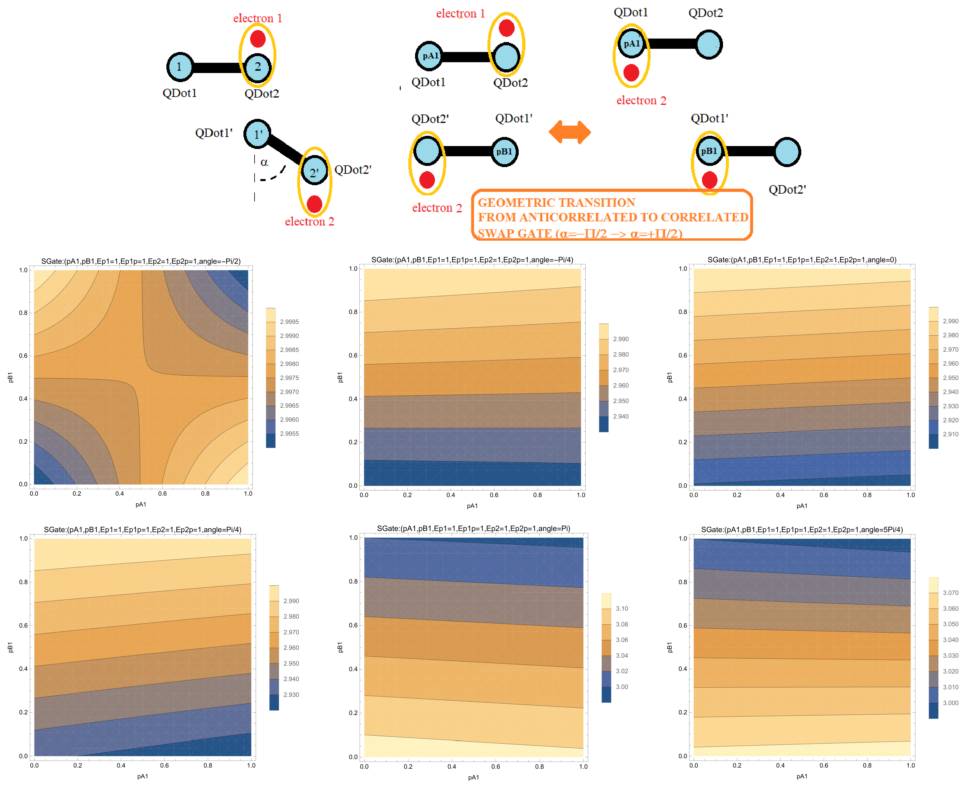
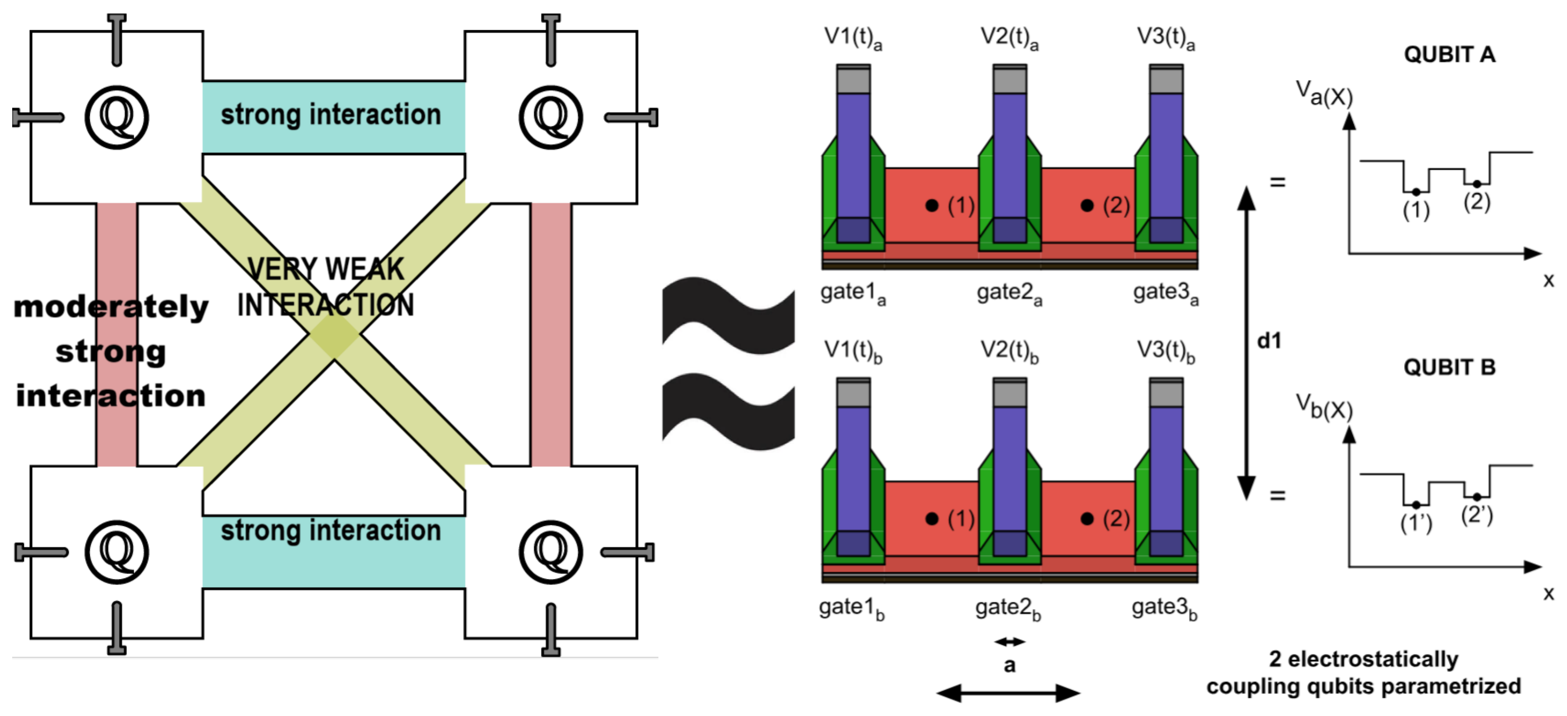

Disclaimer/Publisher’s Note: The statements, opinions and data contained in all publications are solely those of the individual author(s) and contributor(s) and not of MDPI and/or the editor(s). MDPI and/or the editor(s) disclaim responsibility for any injury to people or property resulting from any ideas, methods, instructions or products referred to in the content. |
© 2026 by the authors. Licensee MDPI, Basel, Switzerland. This article is an open access article distributed under the terms and conditions of the Creative Commons Attribution (CC BY) license.