


Abstract
Background: Wearable EEG devices offer an accessible and unobtrusive system for regular brain health monitoring outside clinical settings. However, due to the current lack of data available from wearable low-density EEG devices, we need to anticipate the extraction of biomarkers for brain health evaluation from available clinical datasets. Methods: This study evaluates multiclass dementia classification of Alzheimer’s disease, frontotemporal dementia, and healthy controls using features derived from low-density temporal EEG electrodes as a proxy for wearable EEG setups. The feature set comprises power-based metrics, including the 1/f spectral slope, and complexity metrics such as Hjorth parameters and multiscale sample entropy. Results: Our results show that multiclass differentiation of dementia, using low-density electrode configurations restricted to temporal regions, can achieve results comparable to a full-scalp configuration. Notably, electrode T5, positioned over the left temporo-posterior region, consistently outperformed other configurations, achieving a subject-level accuracy of 83.3% and an F1 score of 82.4%. Conclusions: These findings highlight the potential of single-site EEG measurement for wearable brain health devices.
1. Introduction
Wearable technologies are increasingly being explored for continuous, accessible, unobtrusive monitoring of brain activity outside clinical settings [1]. Among these, ear-EEG has emerged in the last decade as a promising approach, recording EEG [2] using a wearable form factor with electrodes placed in the inner or outer ear [3]. The performance of ear-EEG is comparable to scalp-EEG for temporal electrode recordings [4]; however, further improvement of the signal-to-noise ratio and artefact removal techniques are needed. The embedding of EEG into wearable devices, such as headphones and hearing aids [5,6], could enable regular, at-home monitoring of brain health [7].
The potential of ear-EEG for brain health monitoring has been increasingly explored in recent years. Musaeus et al. [8] demonstrated its feasibility for long-term monitoring of patients with Alzheimer’s disease (AD). Subsequent studies by the same group extended this work to characterise seizure patterns in AD patients using at-home, long-term ear-EEG recordings [9,10]. These studies highlight the potential of wearable EEG systems, such as ear-EEG, for continuous data acquisition outside clinical environments, an approach that could also be leveraged for dementia classification and disease progression monitoring.
The classification of dementia using machine learning models applied to full-scalp EEG data has been extensively explored [11,12,13,14,15,16,17]. Power-based features, looking at the relative power of the different frequency sub-bands (delta, theta, alpha, beta, gamma), were employed successfully (as part of a larger feature set) in [13] for binary classification of AD versus healthy control (HC) (denoted AD/HC), frontotemporal dementia (FTD) versus HC (FTD/HC), and combined dementia subtypes (AD and FTD) versus HC (AD+FTD/HC). Similarly, Ruiz-Gómez et al. [12] and Pérez-Valero et al. [11] incorporated relative power features for multiclass classification of AD, mild cognitive impairment (MCI), and HC. Another power-based metric relevant to dementia classification is the 1/f spectral slope, which captures the power distribution of high-frequency sub-bands to low-frequency sub-bands. A flattening of the slope has been shown to correlate with age-related cognitive decline [18] and can be used as a biomarker for neurodegenerative diseases such as AD [19]. To the best of the authors’ knowledge, aside from their own forthcoming work [20], this metric has not been applied in dementia classification models. Its effectiveness as a feature is further evaluated in this study.
As noted in [21], power-based features may be limited as a metric to differentiate FTD patients from HC and AD. Therefore, this study incorporates complexity-based features, specifically Hjorth parameters and multiscale sample entropy (MSE). The Hjorth parameters (activity, mobility, and complexity) have been implemented in [15] for the binary classification of AD/HC, FTD/HC, and AD+FTD/HC, and in [14] for binary classification of AD/FTD. MSE, a measure for assessing the complexity of a time series across a range of time scales, is used when the data’s time scale of relevance is unknown, as in EEG. MSE has been used in [16] to assess AD/HC and AD/HC+MCI, and in [17] to evaluate AD/HC.
Multiclass dementia classification in the literature, without the use of deep learning, has often been implemented as a series of binary classifications. In one approach, first, a dementia versus HC classification is performed, followed by a binary classification of two dementia subtypes, as in [22]. While this method does achieve strong performance, it does not take into consideration that dementia is an umbrella term encompassing multiple neurodegenerative diseases with shared symptomology [23,24,25]. A true multiclass approach, in which a single model distinguishes all dementia subtypes, may better handle the diversity encountered in clinical settings. This approach could ensure robust handling of overlapping EEG biomarkers observed across neurodegenerative and other neurological disorders. Combining multiclass dementia classification with a classical machine learning method can offer the additional benefit of interpretability, allowing clinicians to understand which features drive the model’s decisions. This transparency is often lacking in deep learning approaches. In clinical applications, the ability to trace diagnostic reasoning back to interpretable EEG features may ultimately improve clinician confidence and facilitate adoption.
In this study, multiclass classification of dementia subtypes (AD and FTD) and healthy controls is implemented using temporal electrode data extracted from full-scalp EEG recordings, evaluating multiple low-density electrode configurations. This approach serves as a proxy for assessing whether low-density EEG, such as ear-EEG, could provide sufficient information for brain health evaluation, and informs electrode selection strategies for future wearable brain health technologies.
2. Materials and Methods
2.1. The Dataset
A publicly available dataset recorded by the 2nd Department of Neurology at the AHEPA General University Hospital of Thessaloniki [26] was used for this study. The dataset consists of EEG recordings taken from 88 individuals (29 healthy controls, 36 individuals diagnosed with AD, and 23 with FTD). AD and FTD were initially diagnosed according to the criteria outlined in the Diagnostic and Statistical Manual of Mental Disorders (3rd edition, revised; DSM-III-R; DSM-IV; ICD-10) [27], and the National Institute of Neurological and Communicative Disorders and Stroke–Alzheimer’s Disease and Related Disorders Association (NINCDS–ADRDA) guidelines [28]. The median disease duration was 25 months, with an interquartile range (IQR; Q1–Q3) of 24–28.5 months.
A 19-electrode Nihon Kohden EEG clinical device (electrode positions: Fp1, F7, F3, T3, C3, T5, P3, O1, Fz, Cz, Pz, Fp2, F4, F8, C4, T4, P4, T6, O2) was used to record the data with a sampling frequency of 500 Hz at rest with eyes closed. The electrodes were positioned according to the 10–20 system configuration, with linked mastoids as reference.
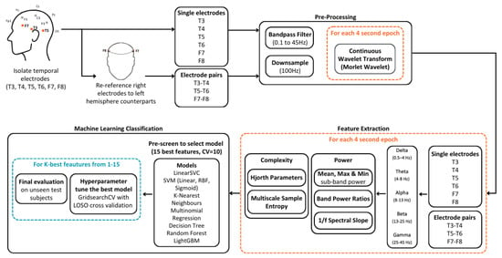
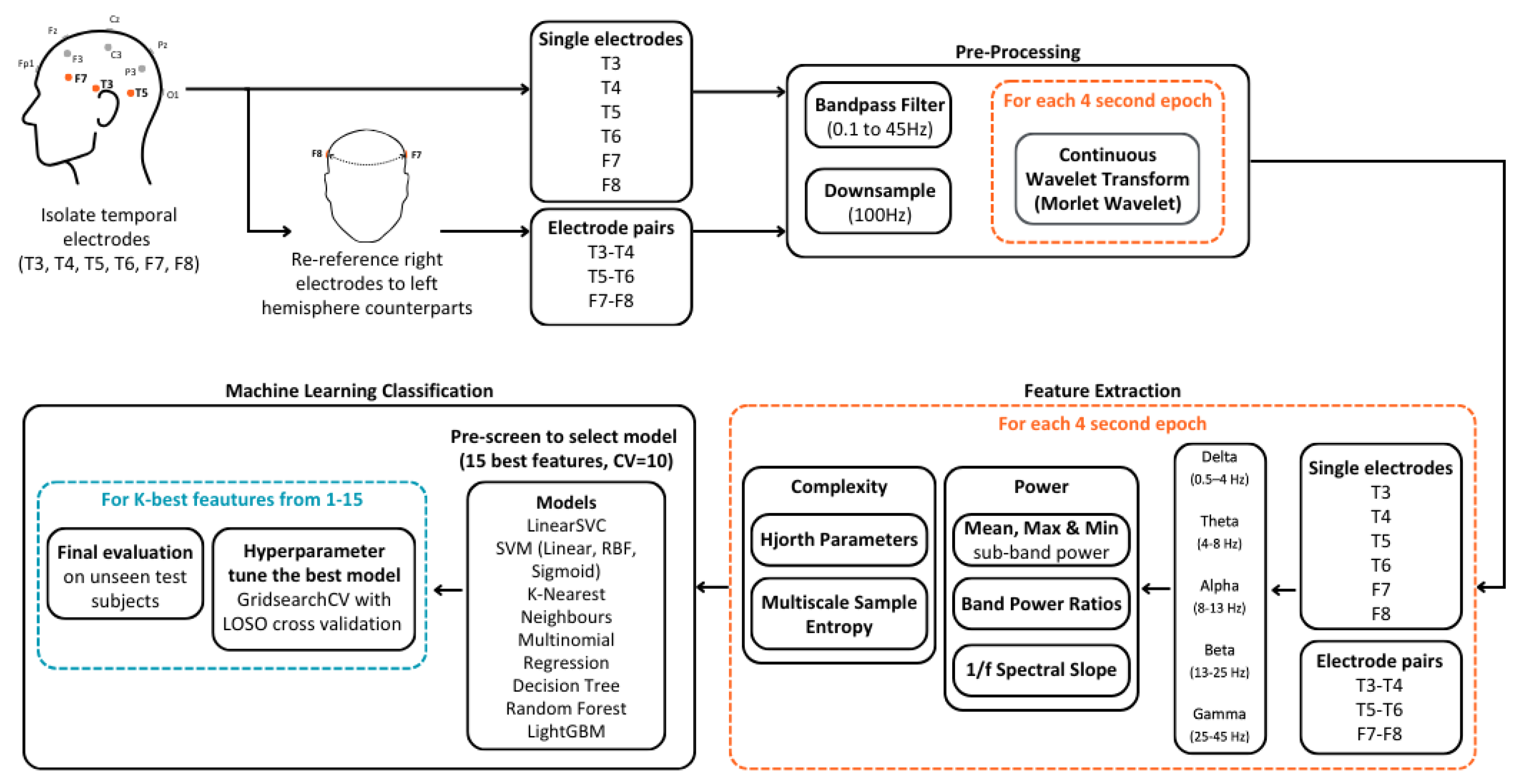
A breakdown of the dataset demographics can be seen in Table 1. Figure 1 shows a graphical summary of the methods employed for our multiclass dementia differentiation, based on low-density temporal electrode EEG data.
Table 1.
Dataset description, including the number of subjects per group, mean age with standard deviation (Std), the mean Mini-Mental State Examination with Std, and the mean EEG recording duration for each group with Std. (MMSE) score with Std.
Figure 1.
Workflow of the proposed approach, including EEG pre-processing, feature extraction, and machine learning classification.
2.2. Pre-Processing
The EEG data from temporal electrodes T3, T4, T5, T6, F7, and F8 were first extracted. Prior to filtering, we created bipolar derivations of temporal electrodes by subtracting left-hemispheric EEG data from their right-hemispheric counterparts. This resulted in three temporal electrode pairs: T3–T4, T5–T6, and F7–F8.
Thus, multiple low-density electrode configurations were considered, consisting of both single temporal electrodes and electrode pair values. These configurations, denoted by C, are defined as follows:
All configurations were subsequently bandpass filtered from 0.1 to 45 Hz and downsampled to 100 Hz.
2.2.1. Bad Data Removal
For each subject, each recording was divided into 4-second epochs, as performed in [11]. Bad data were then identified by kurtosis, a statistical measure that captures the presence of outliers in the signal distribution. First, the kurtosis of each channel C and epoch e was calculated using the kurtosis MATLAB (R2024a) function. Subsequently, the mean and standard deviation was calculated for each channel over all of its epochs as follows:
where E is the set of epochs for channel C. Z-scores () were then calculated epoch-wise for each channel.
Finally, an epoch for a given channel was marked as “bad” if the z-score exceeded a threshold of 3. Channels were fully removed for all epochs if a threshold of 40% or more of its epochs were rejected.
2.2.2. Sub-Band Power Estimation
The continuous wavelet transform (CWT) was performed on each epoch of each channel configuration using the Morlet wavelet. The power of each sub-band for a given epoch was calculated by averaging the squared amplitudes of the wavelet coefficients across the epoch. The sub-bands considered were delta (0.5–4 Hz), theta (4–8 Hz), alpha (8–13 Hz), beta (13–30 Hz), and gamma (30–45 Hz).
2.3. Feature Extraction
The following features were then calculated for each of the low-density electrode configurations C.
2.3.1. Sub-Band Power Metrics
The mean, minimum, and maximum powers for each channel configuration C within each epoch were calculated as follows:
where
- denotes the mean power in sub-band S during epoch e.
- and represent the minimum and maximum sub-band power values, respectively, within epoch e and frequency band S.
- is the complex wavelet coefficient at frequency f and time t for electrode configuration C.
- is the set of discrete frequencies that define the sub-band S.
- is the set of discrete time points within epoch e.
- and represent the cardinalities (i.e., number of elements) of the sets and , respectively.
2.3.2. Band Power Ratios
Ratios between fast and slow band powers were computed for each epoch e and channel configuration C, using the mean sub-band power values , , , and :
For brevity, these ratios are referred to in the text as theta_alpha, theta_beta, theta_alpha_beta, and delta_theta_alpha_beta, respectively.
2.3.3. 1/f Spectral Slope
In addition, the 1/f spectral slope was computed for each epoch and channel configuration C. First, the alpha band was omitted to limit the effects of periodic oscillatory peaks in the slope estimation, as performed in [18]. Then for each sub-band S, the mean epoch power was computed and both frequency and power values were log-transformed. The spectral slope was then obtained by fitting a linear regression between the logarithm of the central frequency of each sub-band and the logarithm of the corresponding mean power.
2.3.4. Hjorth Parameters
The Hjorth parameters, activity, mobility, and complexity, were calculated as follows:
where
- : EEG signal at time t, for epoch e and electrode configuration C.
- : First derivative of the signal.
- : Second derivative of the signal.
2.3.5. Multiscale Sample Entropy
The MSE of each epoch was calculated following the approach described in [17], using a pattern length (m) of 1 and a tolerance (r) of 0.25. The maximum time scale () was selected such that the minimum number of samples in a coarse-grained time series would be 100 samples (). The minimum value of () was chosen to approximately match the number of samples as for high time scales in [16,17].
Each epoch was broken down into non-overlapping segments of length , for . A window of length was slid over the coarse-grained signal. All pairs of length patterns were compared using the Chebyshev distance, and the number of similar pairs (whose distance is less than the tolerance r times the standard deviation) were counted (A). The approach was repeated for length patterns (B). The sample entropy was calculated as follows:
Finally, the slope of the sample entropy values across all time scales in was calculated for the epoch.
2.4. Machine Learning Implementation
2.4.1. Class Balancing
To prepare the data for training, the number of epochs per class was balanced by limiting them to the count of the minority class. For classes with a larger number of epochs, a random subset was selected, using a fixed seed to ensure reproducibility. An epoch-level class balancing approach was chosen over a subject-level balancing method. By balancing at an epoch-level, we avoid removing subjects from the dataset and preserve subject variability in the model.
2.4.2. NaN Handling
Features belonging to epochs that were rejected in the data cleaning process were recorded as NaN. These entries were imputed with the median value of the respective feature for the given subject. As cross-validation folds during the model training process ensure that all epochs from a given subject remain within the same fold, this procedure does not introduce data leakage.
2.4.3. Train–Test Split
An 80–20 train–test split was used. To ensure no data leakage, all epochs belonging to a particular subject were kept in the same split using the GroupShuffleSplit method from scikit-learn. Model selection, hyperparameter tuning, and feature selection were performed exclusively on the training set. The test set was reserved strictly for the evaluation of the final model.
2.4.4. Standardisation of Features
Features were standardised using the scikit-learn StandardScaler transformation, which scales features to have a mean of zero and a standard deviation of one. To prevent introducing bias to the model, the scalar was fitted using only the training set. The resulting parameters (mean and standard deviation for each feature) were then applied to transform the test set.
2.4.5. Model Selection
An initial model pre-screen was performed by assessing the performance of a range of classifiers on datasets derived from single electrodes and electrode pairs. The classifiers evaluated included linear support vector classifier (LinearSVC), linear support vector machine (SVM), radial basis function (RBF) SVM, sigmoid SVM, k-nearest neighbours, multinomial logistic regression, decision tree, random forest, and light gradient boosting model (LightGBM). For the initial screening, the top 15 features were selected using ANOVA, and 10-fold cross-validation was employed to narrow down the more effective modelling approaches.
2.4.6. Hyperparameter Tuning
Hyperparameter tuning was performed on the selected model using nested cross-validation with a Leave-One-Subject-Out (LOSO) approach. In the outer loop, one subject was held out as the validation set in each fold, while the remaining subjects formed the training set. Within the inner loop, stratified group 5-fold cross-validation was used with grid search for hyperparameter tuning. The best-performing model from the inner loop was then evaluated on the held-out subject.
2.4.7. Feature Selection
The LOSO nested validation was repeated for the top k features, where k ranged from 1 to 15. The k features were selected using the SelectKBest scikit-learn function with the f_classif scoring function, which applies ANOVA F-values to rank feature relevance. P-values were clipped to a minimum of and feature importance scores were then computed as . Finally, scores were normalised by dividing by the maximum score across all features, resulting in a relative importance scale between 0 and 1.
2.4.8. Final Model Evaluation
The best model for each electrode configuration and k value was evaluated with the held-out test set. Subject-level group classification was determined based on the majority vote of the predicted classes across all its epochs.
Performance was evaluated by calculating accuracy, recall, precision, specificity and the F1 score, which are defined as follows:
where , , , and represent true positive, true negative, false positive, and false negative predictions, respectively.
In addition, Cohen’s kappa [29] was evaluated, a performance metric which accounts for correct predictions occurring by chance. Cohen’s kappa () is defined as follows:
where and represent the observed and expected agreements, respectively, and are calculated as follows:
where
- Actual pos (positives) = ;
- Actual neg (negatives) = ;
- Predicted pos (positives) = ;
- Predicted neg (negatives) = ;
- N = the total number of samples.
3. Results
3.1. Class Representation in the Train and Test Sets
A detailed breakdown of class representation in the training and test sets is provided in Table 2. The GroupShuffleSplit method was used to allocate 20% of subjects to the test set while ensuring that all epochs from a given subject remained within the same split, thereby preventing data leakage. As shown in Table 2, the resulting class proportions deviate slightly from the 80–20 split. In particular, for the FTD group, 20 subjects (87%) were assigned to the training set, whereas 3 subjects (13%) were included in the test set.
Table 2.
Summary of class representation in the training and test sets at both the epoch and subject levels. The 80–20 train–test split was applied using GroupShuffleSplit, which assigns 20% of subjects to the test set without enforcing class stratification.
3.2. Model Selection
The results of the initial model selection pre-screen are displayed in Table 3 and Table 4 for single electrode and electrode pair configurations, respectively. In order to facilitate direct and fair comparison across both configurations, a single classifier was selected to be used consistently.
Table 3.
Model selection results for single electrode configurations, ordered by the F1 macro score. The mean accuracy, F1 macro score, fit time, and score time are averaged across the folds of a 10-fold cross-validation. The standard deviation (Std) is reported for accuracy and F1 macro scores. The fit time refers to the duration required to train the model, while the score time represents the duration needed to evaluate the model on the held-out validation set.
Table 4.
Model selection results for electrode pair configurations, ordered by the F1 macro score. The mean accuracy, F1 macro score, fit time, and score time are averaged across the folds of a 10-fold cross-validation. The standard deviation (Std) is reported for accuracy and F1 macro scores. The fit time refers to the duration required to train the model, while the score time represents the duration needed to evaluate the model on the held-out validation set.
The top four performing models for both single electrode and electrode pair configurations were multinomial regression, LinearSVC, RBF SVM, and random forest. RBF SVM was omitted from further consideration due to its high training time. Random forest was selected as the final model because it demonstrated strong overall performance, with accuracy/F1 scores of 0.439/0.423 and 0.489/0.476 for single electrode and electrode pair configurations, respectively. Although multinomial regression and LinearSVC outperformed random forest in the single electrode setting, a non-linear model was preferred to capture more complex patterns in the data that linear models may not fully represent.
3.3. Model Performance for Low-Density Electrode Configurations
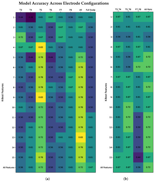
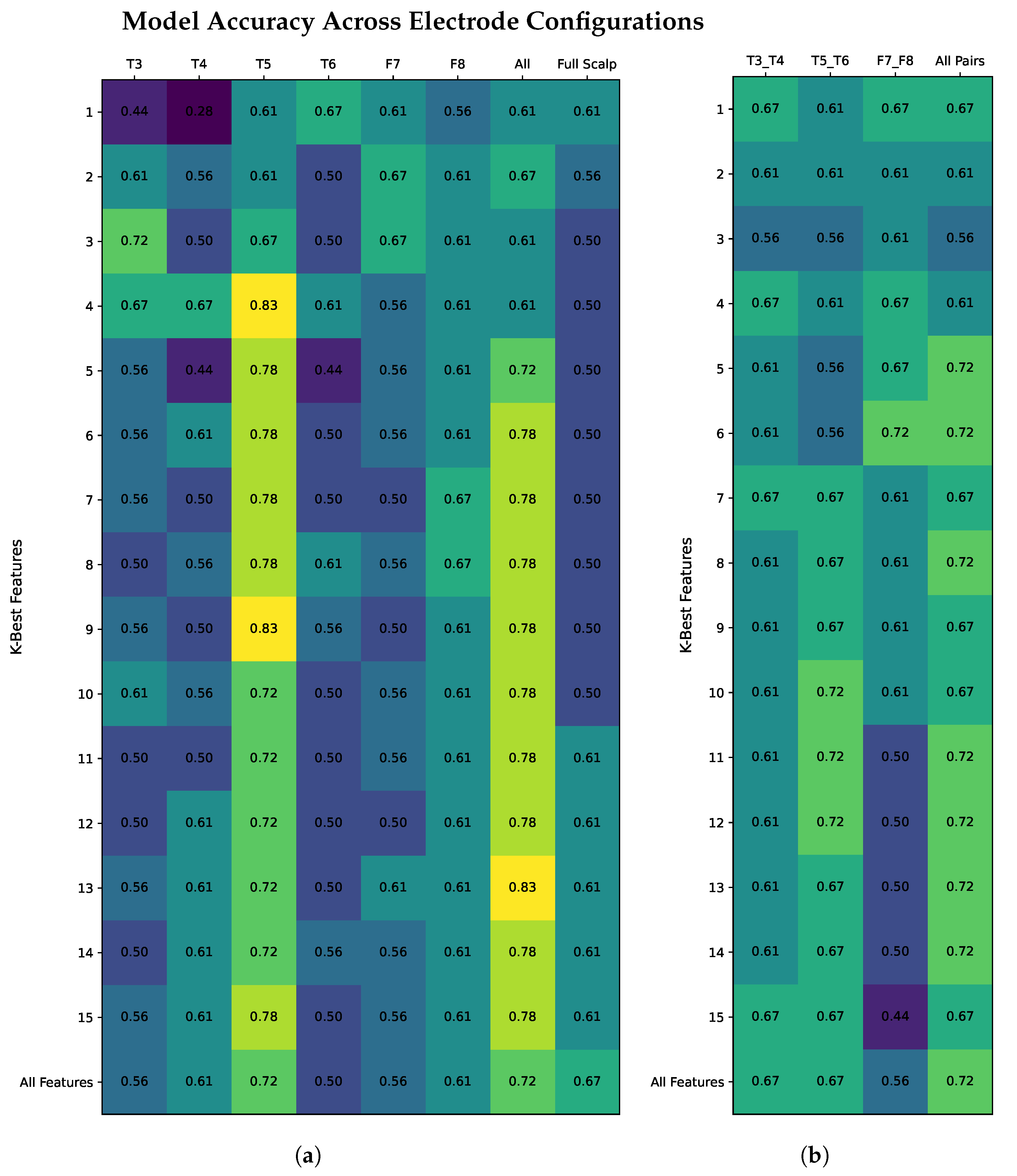
Classification performances for single electrode configurations (T3, T4, T5 T6, F7, and F8) and electrode pair configurations (T3–T4, T5–T6, and F7–F8) using random forest with K best features from 1 to 15 and all features are displayed in Table 5 and Table 6, respectively. A heatmap of the accuracy values for both configurations is shown in Figure 2.
Table 5.
Single electrode classification performance using the K most important features (K = 1–15) and all available features. Accuracy and F1 scores are reported. The “All Single” condition indicates that the model selected the K best features from all temporal electrodes combined, whereas the “Scalp” condition allowed feature selection from the full-scalp dataset comprising 19 electrodes.
Table 6.
Electrode pair classification performance using the K most important features (K = 1–15) and all available features. Accuracy and F1 scores are reported. The “All Pairs” condition indicates that the model selected the K best features from all temporal electrode pairs combined.
Figure 2.
Comparison of model accuracy for single electrode (a) and electrode pair (b) configurations. The scalp bench mark in (a) is obtained by selecting the K best features from the full set of 19 electrodes. Colour intensity indicates model performance, with lighter shades representing higher accuracy and darker shades representing lower accuracy.
The highest single electrode accuracy was achieved using electrode T5, with a maximum accuracy of 0.833 (for K = 4 and K = 9), and a corresponding F1 score of 0.824. Overall, T5 consistently outperformed the other electrodes across most values of K. When models could be built using features from all single temporal electrodes (T3, T4, T5 T6, F7, and F8), a peak accuracy of 0.833 and F1 score 0.800 was reached. Furthermore, for models where features from all 19 scalp electrodes could be selected, the highest accuracy achieved was 0.667 and an F1 score of 0.603 was achieved.
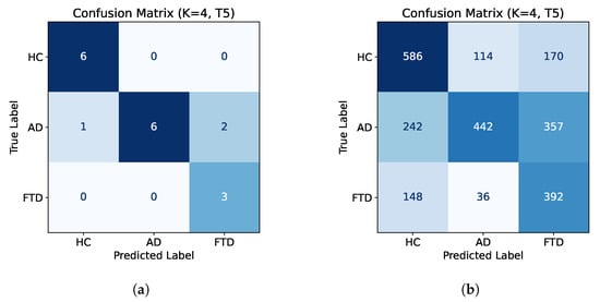
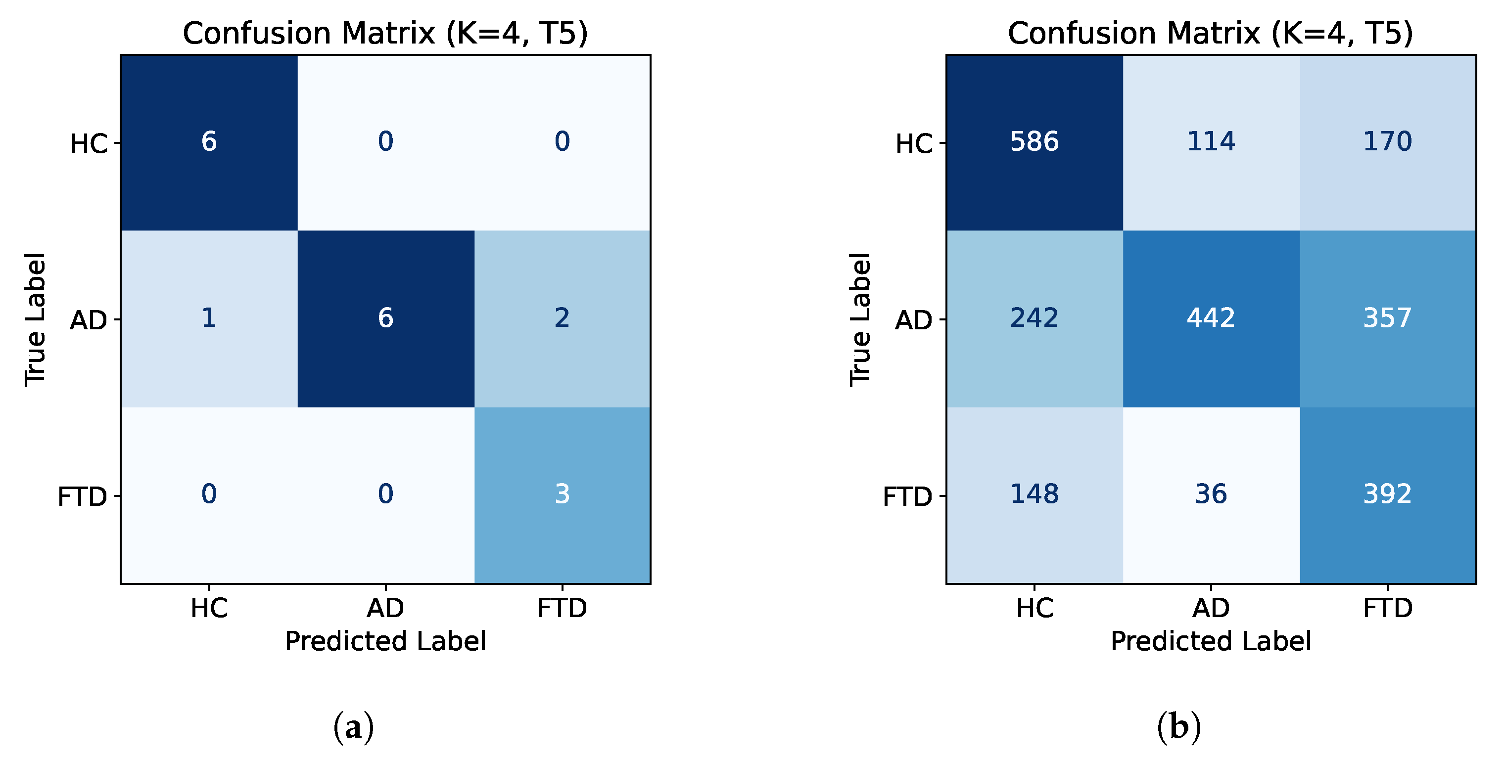
Figure 3 displays confusion matrices for the subject-level classification (Figure 3a) and epoch-level classification (Figure 3b) for electrode T5 with K = 4 best features. A breakdown of the epoch-level classifications and the final subject-level classification of FTD subjects is shown in Table 7. Of the three test subjects with FTD, all three are classified correctly, one with a high confidence level (94%) and the others with lower confidence (55% and 62%, respectively).
Figure 3.
Subject-level confusion matrix for electrode T5 with K = 4 best features (a) and the corresponding epoch-level confusion matrix (b). Subject-level classifications were determined by taking the majority decision of each subject’s epoch-wise classification. Colour intensity represents the number of correctly and incorrectly classified samples (darker colours indicate higher frequency).
Table 7.
Epoch-level classification of FTD test subjects. Each column shows the number of epochs classified as HC, AD, or FTD. The final (subject-level) classification is determined by majority vote across epochs. Confidence is calculated as the proportion of epochs assigned to the final classification label over the total number of epochs.
A comparison of electrode T5’s classification performance using the top-performing models identified during the model pre-screening in Section 3.2 is presented in Table 8. Accuracy and F1 scores are computed based on subject-level majority voting. The random forest model achieved the best subject-level performance in terms of accuracy (0.833), F1 score (0.824), and Cohen’s kappa (0.747). However, the Cohen’s kappa reported based on the classification performance of individual epochs was lowest for random forest (0.367), compared to LinearSVC (0.467) and multinomial regression (0.466).
Table 8.
Comparison of electrode T5’s classification performance (K = 4 features) using the random forest, LinearSVC and multinomial logistic regression models. The performance metrics are the test accuracy and F1 scores (based on subject-level majority voting) and Cohen’s kappa (reported based on both subject-level majority voting and individual epoch classification performance).
Electrode pair classification performance using the random forest classifier was evaluated for three electrode pair configurations, T3–T4, T5–T6, and F7–F8, as well as a configuration allowing selection from all pairwise features. Results for model performance using the K best features (where K = 1 to 15), as well as using all features, are shown in Table 6 and Figure 2b.
Among individual pairs, the strongest performance was yielded from electrode pair T5–T6, achieving a top accuracy of 0.722 and F1 of 0.65 for k = 10. More consistent, although moderate, results were obtained from electrode pair T3–T4, with accuracy and F1 ranging from 0.556–0.667 and 0.538–0.638, respectively. For electrode pair F7–F8, we see that lower k values perform well, achieving an accuracy of 0.722 and an F1 of 0.648 at k = 6. However, performance for higher values of k is low, with a minimum accuracy and F1 of 0.444 and 0.389, respectively, at k = 15.
3.4. Feature Importance
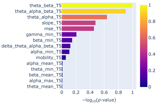
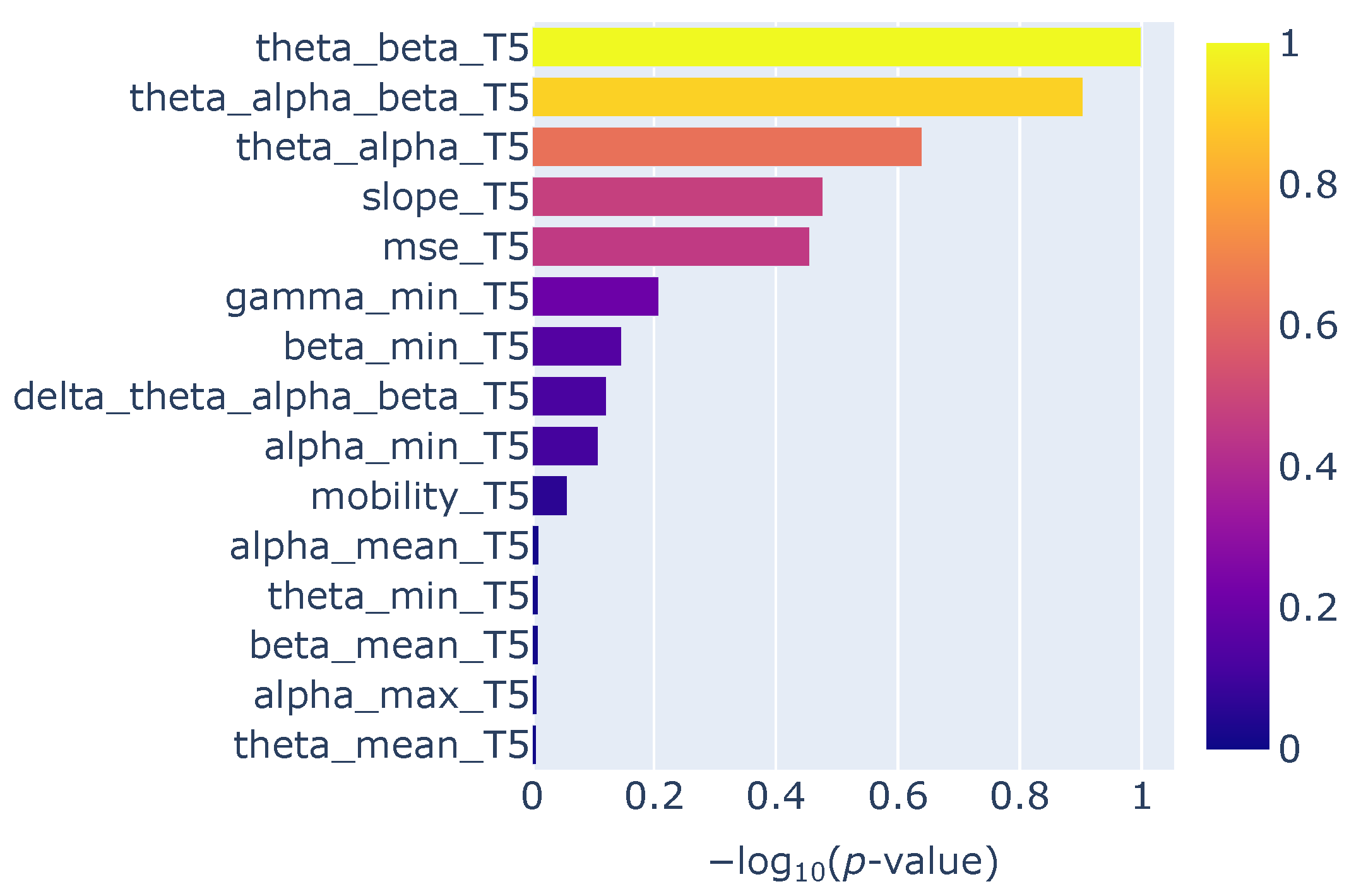
Feature importance analysis for electrode T5, based on SelectKBest using ANOVA F-value scoring, is presented in Table 9 and Figure 4. The most discriminative feature was the band power ratio of theta to beta power (theta_beta_T5) with a p-value of p-value of and a normalised importance score of . The second most informative feature was the ratio of theta to the combined alpha and beta power (theta_alpha_beta_T5), followed by the ratio of theta to alpha power (theta_alpha_T5) and the 1/f spectral slope, which achieved normalised scores of 0.9036, 0.6404, and 0.4771, respectively.
Table 9.
Electrode T5 feature importance using SelectKBest with ANOVA scoring.
Figure 4.
Feature importance for electrode T5.
3.5. Channel Quality
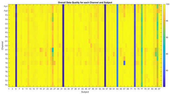
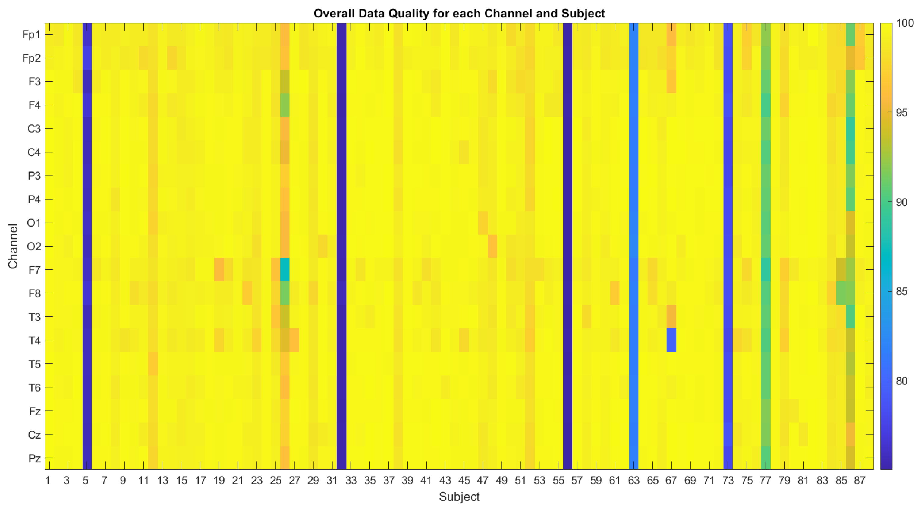
In order to investigate whether the consistent superior classification performance of channel T5 was caused by a higher channel recording quality, the quality of all channels was assessed according to the method outlined in [30]. The results in Figure 5 show the overall data quality metric (ODQ) of each channel, which considers the ratio of no-signal windows, high-amplitude windows, high-frequency noise windows, and low-correlation windows. The ODQ ranges from 0% (no good windows of data) to 100% (all windows of good quality). Table 10 shows the average ODQ for each channel across subjects in each group (HC, AD, and FTD).
Figure 5.
Overall data quality for each channel by subject, with quality scores ranging from 75% good windows of data to 100%.
Table 10.
Mean ODQ for each channel across subjects in each group.
As shown in Figure 5, several subjects exhibit lower ODQ scores, indicated in blue. This was driven by a high noise-to-signal ratio (NSR), which was measured by applying a high-pass Butterworth filter at 30 Hz to isolate high-frequency components, followed by computing the variance ratio of the noise to the raw signal in 1 s windows. Windows were labelled as “bad” if the NSR exceeded 5 standard deviations from the mean. As the ODQ scores of these subjects was above 75%, they were kept in the dataset for the remainder of the analysis.
4. Discussion
4.1. Dementia Classification from EEG Data
This study attempted a multiclass approach for dementia classification using a classical machine learning model (random forest) with interpretable features extracted from temporal EEG electrode configurations, with the aim of informing the feasibility of low-density EEG in brain health monitoring applications. Low-density electrode configurations were drawn from temporal electrodes (T3, T4, T5, T6, F7, and F8) to investigate whether low-density EEG, such as ear-EEG, could provide sufficient information for dementia classification. Temporal electrodes were chosen due to their proximity to the ear where volume conduction allows them to approximate signals measurable by ear-EEG.
The highest classification performance was obtained with electrode T5, achieving 83.3% accuracy and an F1 score of 82.4% using K = 4 best features. While the classification confidence for some FTD subjects was relatively low (Table 7), it is noteworthy that the predicted labels remained consistent across most K values. In a clinical context, it would be inappropriate to base an AD/FTD diagnosis on a single 4-second EEG segment, which is why the majority vote across multiple epochs is considered here for comparison.
A summary of the relevant literature is provided in Table 11. Examples [13,14,15,21,22] use the same Thessaloniki dataset as in this study and calculate features using all 19 electrodes.
Table 11.
Comparison of EEG-based machine learning approaches for AD versus FTD classification in the literature.
Pseudo-multiclass classification of AD, FTD, and HC has been explored in the literature through a series of sequential binary classifications [22]. With such an approach, binary classification of combined dementia versus control is first performed (AD+FTD/HC), followed by a secondary binary classifier to separate the dementia subtypes (AD/FTD) if the first stage identifies a dementia case. While this strategy can yield strong performance, for robust dementia classification, models should be designed to handle a broader range of dementia subtypes and account for EEG biomarker similarities with other neurological disorders. Such considerations are essential in order for models to be clinically reliable.
A true multiclass approach was explored in [31] using a long short-term model (LSTM) for the classification of AD, FTD, Lewy body dementia (LBD), progressive supranuclear palsy (PSP), vascular dementia (VAD), and HC. An accuracy of 98.0% was achieved, demonstrating the potential of deep learning methods to successfully handle an array of dementia subtypes in a single unified framework. However, a challenge remains with such approaches in ensuring model interpretability for deployment in clinical environments. As noted in [32], a lack of explainability from “black box models” is a key barrier to the adoption of artificial intelligence (AI) in clinical settings.
A true multiclass approach was also used in our previous work [20]. In this study, we investigated asymmetry in power-based metrics, where the lateralised power for each electrode pair was calculated by subtracting the corresponding electrode power values in the left and right hemispheres. This approach achieved an epoch-wise accuracy of 63.8% and an F1 score of 58.0% for multiclass dementia classification. In the present study, we removed the lateralised power calculation, so that electrode pairs in this work instead represent temporal electrodes re-referenced to their contralateral counterparts. The key methodological difference is the stage at which the contralateral subtraction was applied: whereas in our previous work subtraction was performed after power calculation, in this study the raw EEG signals were first subtracted between contralateral pairs, followed by standard pre-processing steps. We also aimed to build upon our original work by introducing complexity measures, such as Hjorth parameters and MSE, with the expectation that they might further improve classification performance.
4.2. Feature Selection
The highest classification performance was obtained with electrode T5 using the top K = 4 features, as presented in Table 5. These features were theta_beta_T5, theta_alpha_beta_T5, theta_alpha_T5, and slope_T5, as shown in Figure 4.
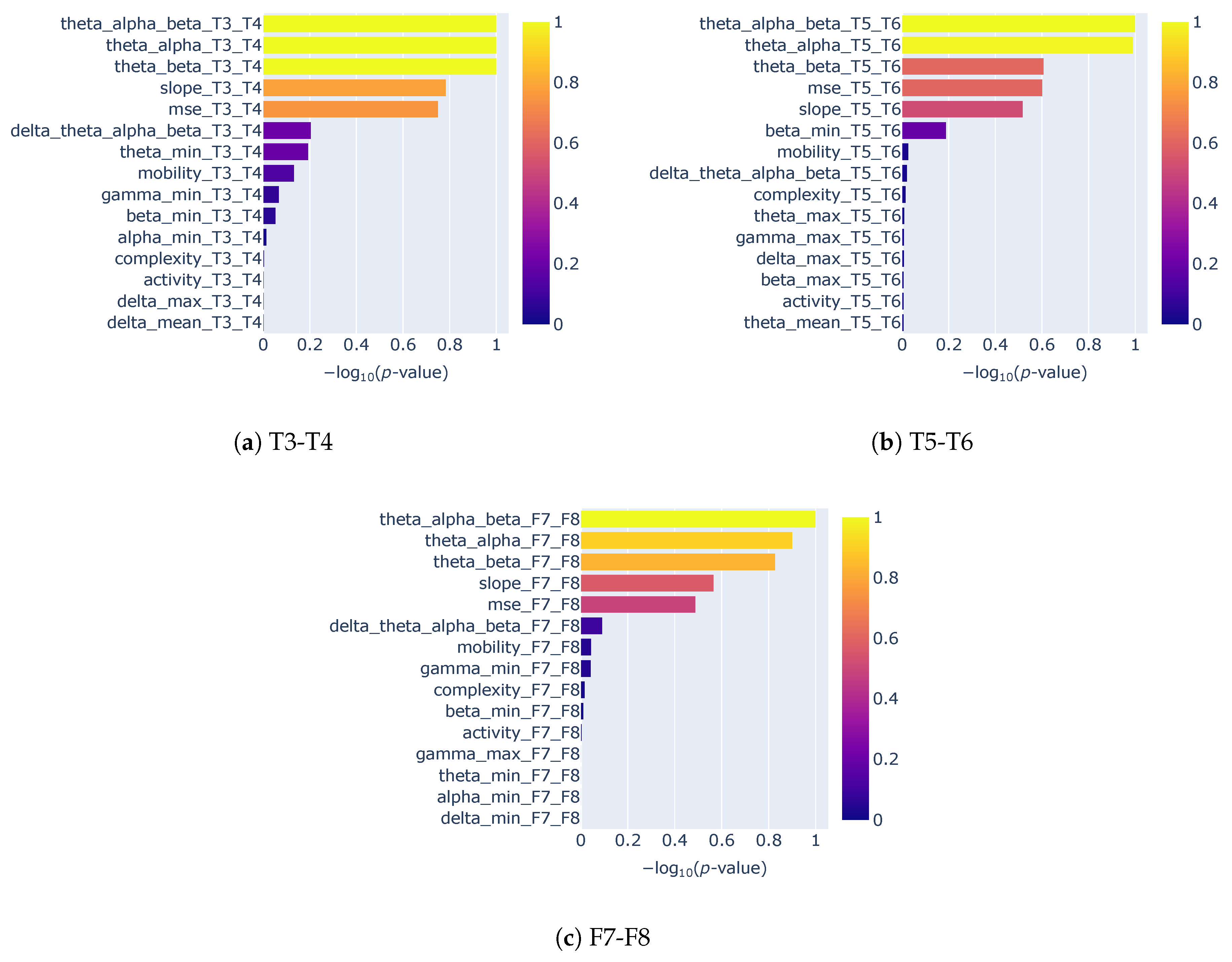
Across single electrode configurations (Figure A5), the power ratio metrics theta_alpha_beta, theta_beta, and theta_alpha consistently achieved the highest rankings. The 1/f spectral slope, used here for the first time in dementia classification to our knowledge, also ranked highly across electrodes in terms of discriminative power. Its high feature importance may reflect its ability to capture broadband spectral changes, including gamma-band alterations, which are not included in any of the band power ratio metrics. This observation aligns with the findings of Chang et al. [33], who showed that the temporal beta-to-gamma power ratio consistently achieved high discriminative performance in distinguishing FTD from HC. For electrode T5, the minimum gamma power ranked as the sixth most important feature. Although gamma power metrics generally exhibited lower discriminative performance across most electrode configurations, at least one gamma-related feature consistently appeared among the top 15 features in both single electrode configurations (Figure A5) and electrode pair configurations (Figure A6).
Complexity measures such as Hjorth parameters and MSE generally showed lower discriminative power than band power ratios in our analysis, although they frequently appeared within the top 15 ranked features. Notably, MSE appeared in the top five features for all electrode pair configurations and for single electrode configurations T3, T5, and T6. The poorer performance of Hjorth parameters was unexpected, as Hjorth parameters achieved strong performance in [13,15] for differentiating dementia from HC (AD+FTD/HC), and in [14] for binary AD/FTD classification, as shown in Table 11. Alternative complexity metrics should be further explored in future work, such as the use of multiscale fuzzy entropy, which has been shown to be more robust for short time series [34].
Functional connectivity (FC) metrics have also demonstrated strong performance as features in the differentiation of AD and FTD in prior work, with accuracies of 84.6% and 96.6% achieved in [22] and [21], respectively. Furthermore, a recent study looking into early detection of brain health decline found that temporal FC was reduced in healthy individuals with pathological amyloid-beta and tau levels [35]. While further investigation is required to determine whether connectivity-based measures can retain their discriminative power when derived from sparse, wearable-friendly EEG configurations, these studies collectively underscore the promise of FC as a feature for wearable brain health applications.
Overall, our feature importance analysis indicates that even with low-density EEG configurations, a small subset of spectral features, particularly sub-band power ratios, the 1/f spectral slope and MSE, can achieve competitive classification performance. Improvement in performance, particularly the model’s ability to discriminate FTD, might be achieved by exploring the use of additional features such as multiscale fuzzy entropy and FC.
4.3. Optimal Electrode Placement for Dementia Classification
Classification results using electrode T5 consistently outperformed both other single electrode and electrode pair configurations. Observing the ODQ channel quality metric for each channel shown in Table 10, the quality of data from channel T5 is similar to other temporal channels and all other scalp channels. This rules out superior channel quality as a possible reason for the increased performance.
Electrode T5 is positioned over the left posterior temporal region. In the temporal variant of FTD, atrophy typically involves the anterior temporal cortex, posterior ventromedial frontal cortex, and temporo-occipital gyri [36]. This atrophy is often asymmetric, and possibly more dominant in the left anterior temporal lobe. However, while the atrophy often begins unilaterally, it generally progresses to involve the contralateral temporal lobe as the disease progresses.
In AD pathology, changes occur in the temporo-parietal cortex, including left angular gyrus atrophy [37] and hypometabolism at the temporo-parietal junction [38]. As electrodes T5 and T6 record from this region, such pathology may account for the enhanced classification performance observed here—particularly for T5, which is better positioned to detect alterations in the left angular gyrus.
As previously mentioned, temporal variant FTD involves asymmetric atrophy in the anterior temporal cortex [36]. As electrodes F7 and F8 are placed over this region, it was expected that they would demonstrate a strong discriminative power for the multiclass classification AD/FTD/HC. However, when used individually, these electrodes achieved only moderate performance, with a maximum accuracy of 66.7% for both F7 and F8. As an electrode pair, F7–F8, a higher accuracy of 72.2% is achieved, although accuracy varies across the different K-best feature configurations and notably decreases for higher values of K.
It should be noted that even when electrodes are placed over regions relevant to a given dementia, volume conduction will cause signals from other brain areas to be detected, although with a stronger contribution from the target region. This should be considered when interpreting electrode-specific performance.
4.4. Clinical Impact
In this study, we present a framework for deriving a dementia multiclass classification model for low-density EEG configurations. We aim to build on the robustness of our proposed framework by including a broader range of datasets (including other dementia types and neurological conditions), and expanding the feature set to explore metrics such as temporal FC. While EEG is not the current standard for diagnosing dementia, the findings of this study highlight the potential for low-density, wearable EEG systems to complement existing clinical assessments. With further development, wearable EEG could provide a non-invasive and accessible tool for cognitive health, enabling early screening and longitudinal monitoring [1,7,8].
4.5. Limitations and Future Work
While this study has shown the potential for low-density EEG multiclass dementia classification, there are still limitations that should be considered. The sample size was relatively small, comprising only 88 individuals with recordings taken from patients in Greece. To ensure that models generalise robustly to unseen patients, a larger sample size is needed, with representation from multiple demographic and cultural backgrounds. Future work could address this by incorporating additional publicly available dementia datasets and ensuring a diverse demographic representation.
Moreover, details regarding the medications taken by AD and FTD cohorts, as well as changes in executive functions and individual disease duration, are not provided in the dataset used in this study. Their inclusion in future datasets would provide a more comprehensive understanding of model behaviour.
In addition, we built our models using only AD and FTD dementia types. While this represents an initial step toward multiclass dementia classification, future work should incorporate datasets that include additional dementia subtypes, such as vascular dementia and dementia with Lewy bodies. This would ensure broader applicability and improve the robustness of the models. Furthermore, model robustness should also be validated by testing against cohorts with other neurological disorders, as these might share EEG biomarkers that would effect model discrimination.
It should also be noted that the SelectKBest scikit-learn function used to calculate feature importance does not correct for multiple comparisons. Thus, the p-values are used for feature ranking only and are not used here as measures of statistical significance. Further analysis of feature importance using methods such as SHAP values and permutation importance will be explored in future work to compare and validate findings against the current K-best feature analysis.
Furthermore, although class balancing was implemented to ensure that the total number of epochs for each class was uniform, the GroupShuffleSplit method applied to partition the data into training and test sets does not account for class stratification. Instead, it allocates 20% of all subjects to the test set regardless of class label. Our approach prioritised uniformity in the number of epochs per class, rather than constraining the number of subjects to that of the minority class. Consequently, while the overall subject split adheres to an 80–20 ratio, the distribution of subjects within each class across the splits does not strictly follow this ratio. In future work, we plan to perform the 80–20 split within each class independently and then concatenate the resulting train and test sets, thereby ensuring consistent class proportions in both sets.
This study used low-density electrode configurations drawn from temporal EEG sites as a proxy for wearable EEG, such as ear-EEG. This approach was adopted because acquiring a sufficiently large ear-EEG dataset for machine learning applications is currently impractical. Future work will refine this approach by projecting scalp-EEG signals to ear-EEG representations, validated against recorded ear-EEG data.
5. Conclusions
This study investigated the feasibility of performing multiclass classification on EEG data to differentiate AD, FTD, and HC using low-density temporal electrode configurations, with the aim of informing electrode placement strategies for future wearable brain health devices. To ensure better model interpretability, only classical machine learning methods were considered. A random forest model was employed with a subset of interpretable features, including band power ratios, the 1/f spectral slope, MSE, and Hjorth parameters. Results showed that electrode T5 consistently outperformed other electrode configurations despite having similar channel quality. The findings from this study supports the hypothesis that reduced electrode configurations, particularly a single electrode in the left temporo-posterior region, could be sufficient for use in wearable brain health devices. However, further analysis and generalisation study through additional datasets and comparisons across different EEG referencing methods need to be performed to fully support this hypothesis.
Future work will extend beyond dementia classification towards the development of a brain health metric derived from ear-EEG data, enabling longitudinal tracking of cognitive function as individuals age. Such advancements could allow for regular, accessible, and non-invasive brain health monitoring in everyday settings.
Author Contributions
A.W., S.S. and A.L.V. designed the study; A.W. performed the data analysis; A.W. wrote the manuscript; S.S. and A.L.V. revised the manuscript. All authors have read and agreed to the published version of the manuscript.
Funding
This research was supported by grants from NVIDIA and utilised NVIDIA RTX A5000 GPU.
Data Availability Statement
The dataset used in this study is publicly available on the OpenNeuro repository at https://openneuro.org/datasets/ds004504/versions/1.0.7, accessed on 10 October 2024.
Acknowledgments
We would like to acknowledge Maria Kambongi and Loretta Wilson, fellows at the Global Brain Health Institute (GBHI), for their clinical review of our work. We also thank Maria Kambongi, a neurophysiologist, for reviewing the raw EEG data.
Conflicts of Interest
The authors declare no conflicts of interest.
Abbreviations
The following abbreviations are used in this manuscript:
| AD | Alzheimer’s disease |
| FTD | Frontotemporal dementia |
| HC | Healthy control |
| MSE | Multiscale sample entropy |
| ODQ | Overall data quality |
| KNN | K-nearest neighbours |
| SVM | Support vector machine |
| LDA | Linear discriminant analysis |
| SVD | Singular value decomposition |
| FC | Functional connectivity |
Appendix A. Subject- and Epoch-Level Classification Performance
Figure A1.
Subject-level confusion matrices for single electrode configurations using K = 4 best features. Colour intensity represents the number of correctly and incorrectly classified samples (darker colours indicate higher frequency).
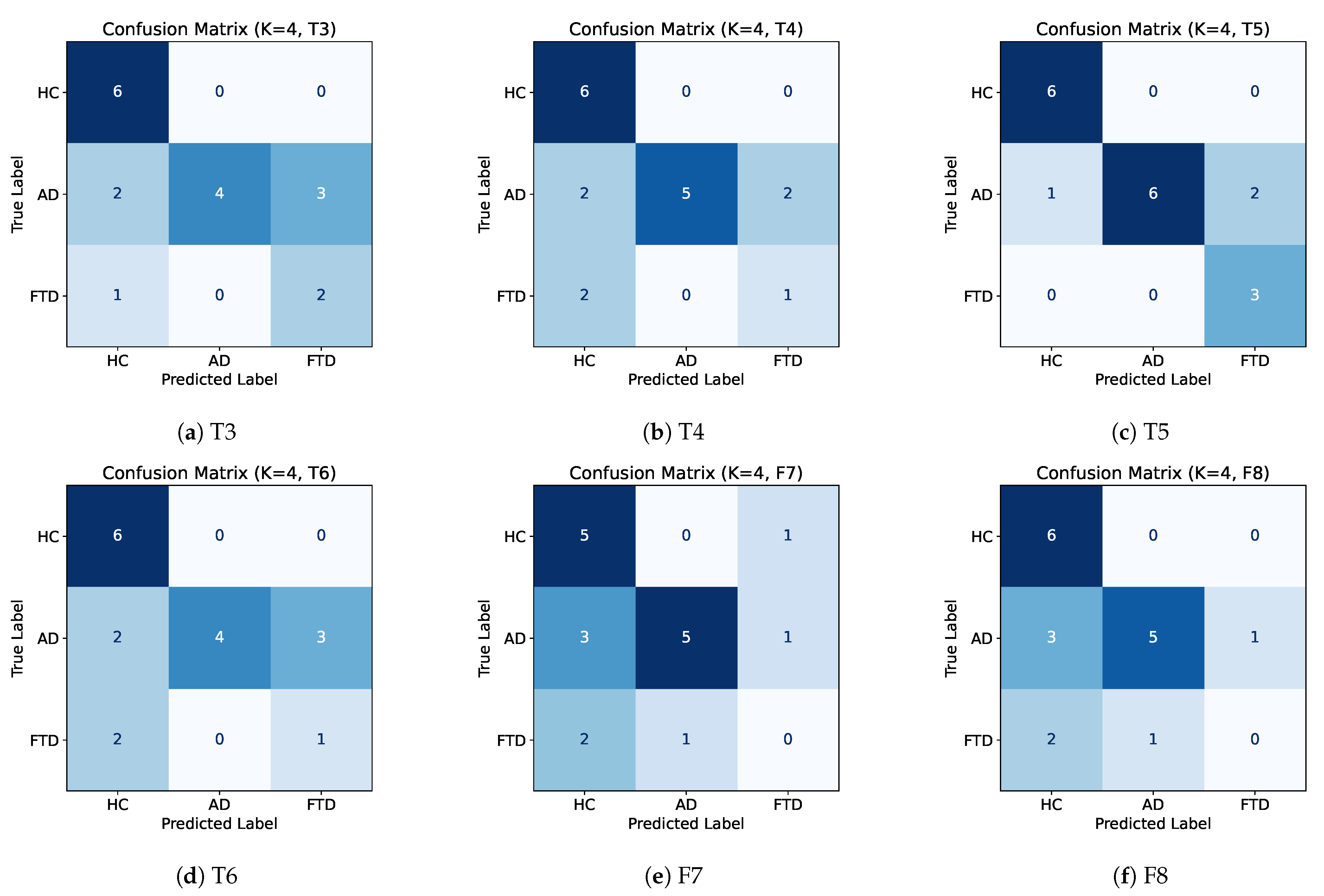
Figure A2.
Epoch-level confusion matrices for single electrode configurations using K = 4 best features. Colour intensity represents the number of correctly and incorrectly classified samples (darker colours indicate higher frequency).
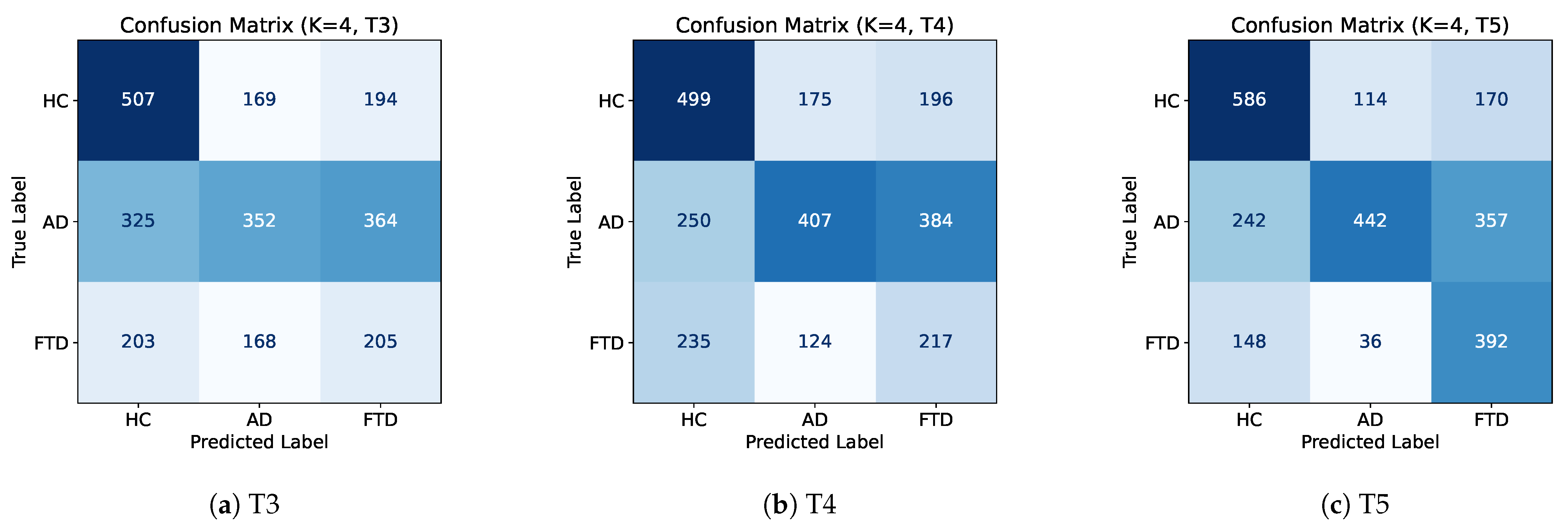
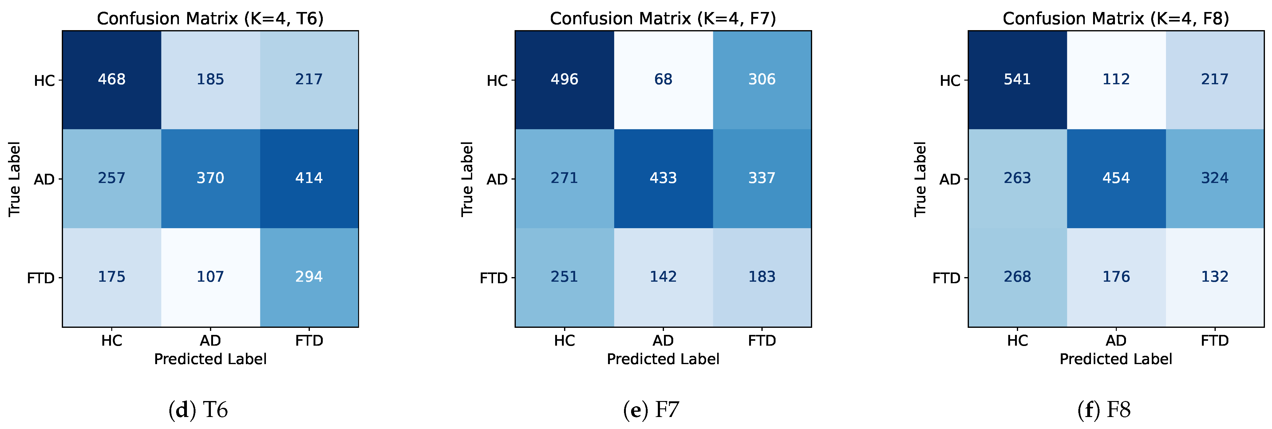
Figure A3.
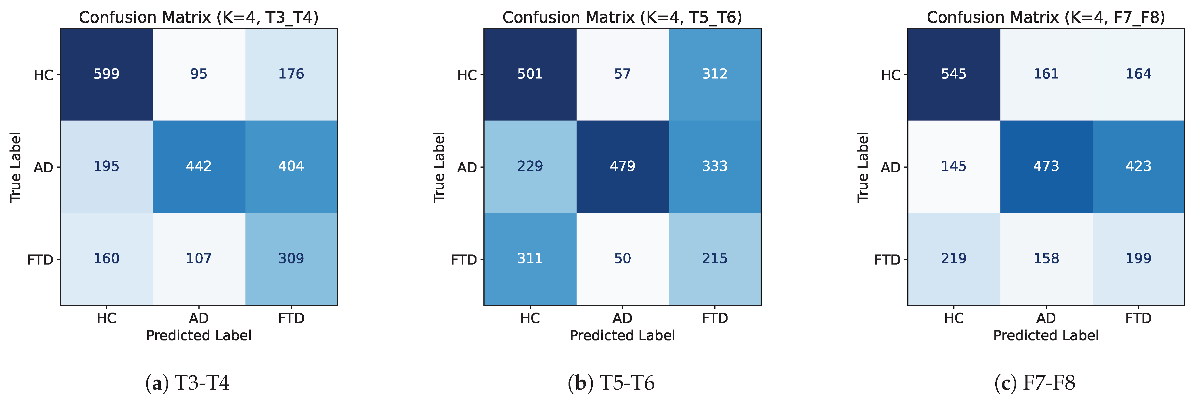
Subject-level confusion matrices for electrode pair configurations using K = 4 best features. Colour intensity represents the number of correctly and incorrectly classified samples (darker colours indicate higher frequency).
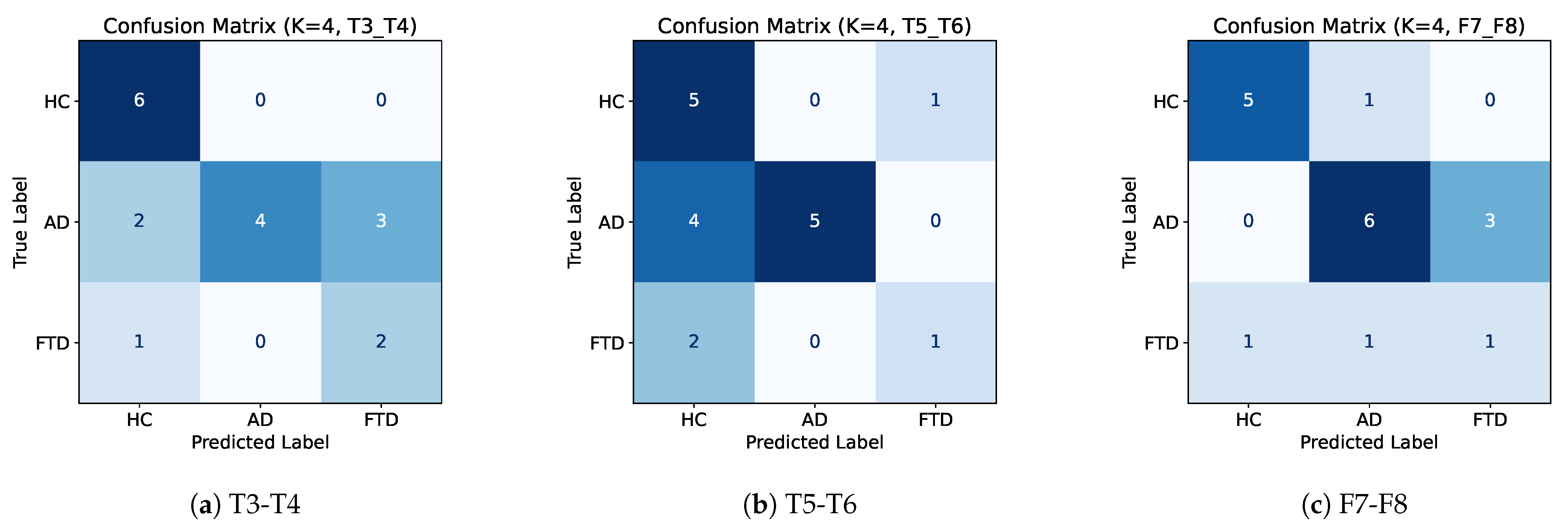
Figure A4.
Epoch-level confusion matrices for electrode pair configurations using K = 4 best features. Colour intensity represents the number of correctly and incorrectly classified samples (darker colours indicate higher frequency).
Appendix B. Feature Importance
Figure A5.
Feature importance for single electrode configurations.
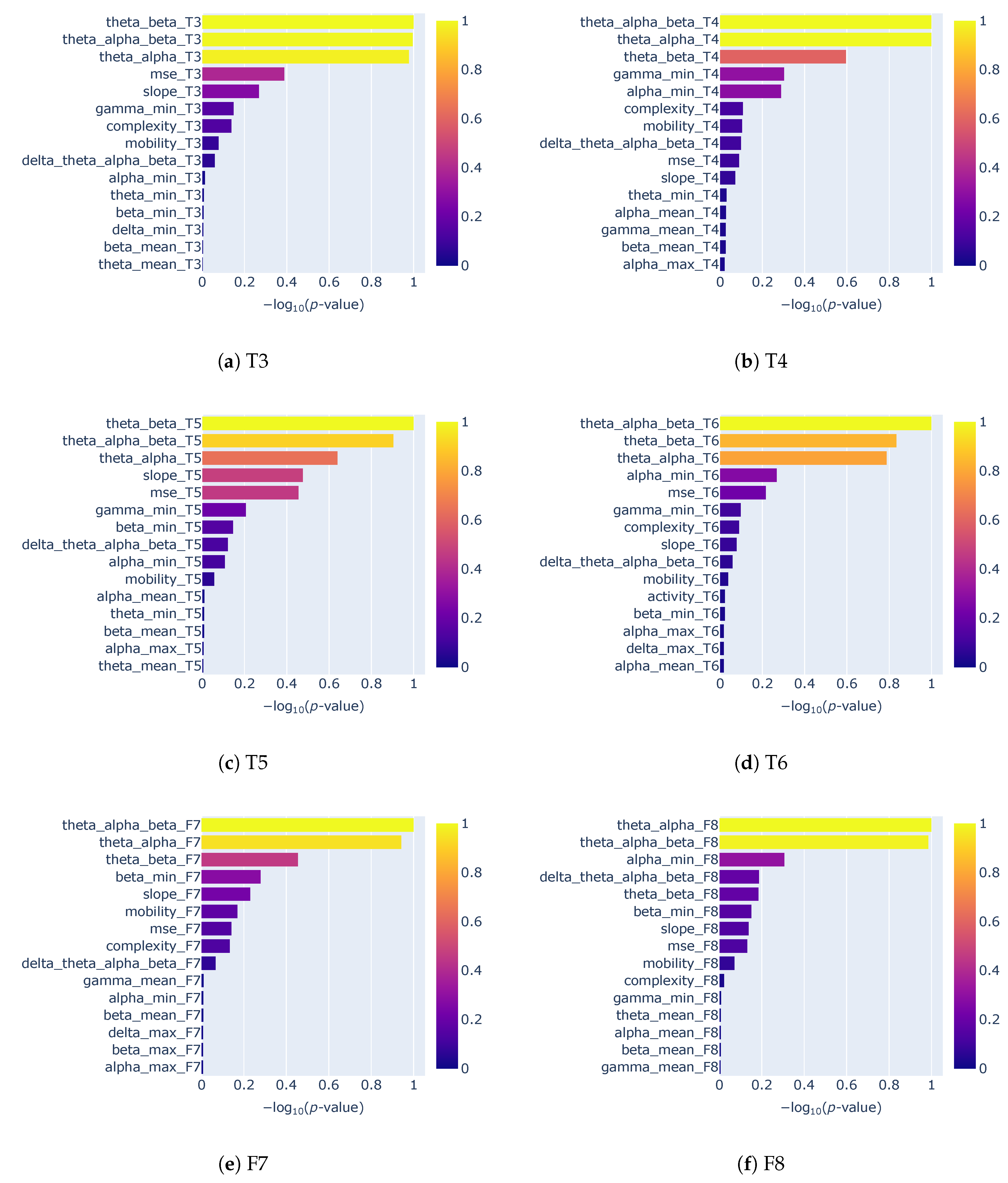
Figure A6.
Feature importance for electrode pair configurations.
References
- Sugden, R.J.; Pham-Kim-Nghiem-Phu, V.L.L.; Campbell, I.; Leon, A.; Diamandis, P. Remote collection of electrophysiological data with brain wearables: Opportunities and challenges. Bioelectron. Med. 2023, 9, 12. [Google Scholar] [CrossRef] [Scilit]
- Berger, H. Über das Elektrenkephalogramm des Menschen. Arch. FÜR Psychiatr. Nervenkrankh. 1929, 87, 527–570. [Google Scholar] [CrossRef] [Scilit]
- Mikkelsen, K.B.; Kidmose, P.; Hansen, L.K. On the keyhole hypothesis: High mutual information between ear and scalp EEG. Front. Hum. Neurosci. 2017, 11, 341. [Google Scholar] [CrossRef] [Scilit]
- Kidmose, P.; Looney, D.; Ungstrup, M.; Rank, M.L.; Mandic, D.P. A study of evoked potentials from ear-EEG. IEEE Trans. Biomed. Eng. 2013, 60, 2824–2830. [Google Scholar] [CrossRef] [Scilit]
- Kaongoen, N.; Choi, J.; Woo Choi, J.; Kwon, H.; Hwang, C.; Hwang, G.; Kim, B.H.; Jo, S. The future of wearable EEG: A review of ear-EEG technology and its applications. J. Neural Eng. 2023, 20, 051002. [Google Scholar] [CrossRef] [Scilit]
- Röddiger, T.; Clarke, C.; Breitling, P.; Schneegans, T.; Zhao, H.; Gellersen, H.; Beigl, M. Sensing with Earables: A Systematic Literature Review and Taxonomy of Phenomena. Proc. ACM Interact. Mob. Wearable Ubiquitous Technol. 2022, 6, 135. [Google Scholar] [CrossRef] [Scilit]
- Kounios, J.; Fleck, J.I.; Zhang, F.; Oh, Y. Brain-age estimation with a low-cost EEG-headset: Effectiveness and implications for large-scale screening and brain optimization. Front. Neuroergonom. 2024, 5, 1340732. [Google Scholar] [CrossRef] [Scilit]
- Musaeus, C.S.; Waldemar, G.; Andersen, B.B.; Høgh, P.; Kidmose, P.; Hemmsen, M.C.; Rank, M.L.; Kjær, T.W.; Frederiksen, K.S. Long-Term EEG Monitoring in Patients with Alzheimer’s Disease Using Ear-EEG: A Feasibility Study. J. Alzheimer’s Dis. 2022, 90, 1713–1723. [Google Scholar] [CrossRef] [Scilit]
- Musaeus, C.S.; Waldemar, G.; Larsson, H.B.W.; Andersen, B.B.; Høgh, P.; Kidmose, P.; Hasselbalch, S.G.; Fabricius, M.; Tøpholm, R.; Rank, M.L.; et al. Detecting seizure patterns in patients with Alzheimer’s disease using long-term EEG monitoring: A feasibility study. Alzheimer’s Dement. 2020, 16, e042025. [Google Scholar] [CrossRef] [Scilit]
- Musaeus, C.S.; Frederiksen, K.S.; Andersen, B.B.; Høgh, P.; Kidmose, P.; Fabricius, M.; Hribljan, M.C.; Hemmsen, M.C.; Rank, M.L.; Waldemar, G.; et al. Detection of subclinical epileptiform discharges in Alzheimer’s disease using long-term outpatient EEG monitoring. Neurobiol. Dis. 2023, 183, 106149. [Google Scholar] [CrossRef] [Scilit]
- Perez-Valero, E.; Lopez-Gordo, M.A.; Gutierrez, C.M.; Carrera-Munoz, I.; Vilchez-Carrillo, R.M. A self-driven approach for multi-class discrimination in Alzheimer’s disease based on wearable EEG. Comput. Methods Programs Biomed. 2022, 220, 106841. [Google Scholar] [CrossRef] [Scilit]
- Ruiz-Gomez, S.J.; Gomez, C.; Poza, J.; Gutierrez-Tobal, G.C.; Tola-Arribas, M.A.; Cano, M.; Hornero, R. Automated Multiclass Classification of Spontaneous EEG Activity in Alzheimer’s Disease and Mild Cognitive Impairment. Entropy 2018, 20, 35. [Google Scholar] [CrossRef] [Scilit]
- Miltiadous, A.; Tzimourta, K.D.; Aspiotis, V.; Afrantou, T.; Tsipouras, M.G.; Giannakeas, N.; Glavas, E.; Tzallas, A.T. Enhanced Alzheimer’s disease and Frontotemporal Dementia EEG Detection: Combining lightGBM Gradient Boosting with Complexity Features. In Proceedings of the 2023 IEEE 36th International Symposium on Computer-Based Medical Systems (CBMS), L’Aquila, Italy, 22–24 July 2023; pp. 876–881. [Google Scholar] [CrossRef] [Scilit]
- Lal, U.; Chikkankod, A.V.; Longo, L. A Comparative Study on Feature Extraction Techniques for the Discrimination of Frontotemporal Dementia and Alzheimer’s Disease with Electroencephalography in Resting-State Adults. Brain Sci. 2024, 14, 335. [Google Scholar] [CrossRef] [Scilit]
- Lee, D.G.; Lee, S.B. Diagnosis of Alzheimer’s Disease and Frontotemporal Dementia From Electroencephalography Signals. IEEE Trans. Neural Syst. Rehabil. Eng. 2025, 33, 2160–2169. [Google Scholar] [CrossRef] [Scilit]
- Maturana-Candelas, A.; Gómez, C.; Poza, J.; Pinto, N.; Hornero, R. EEG characterization of the Alzheimer’s disease continuum by means of multiscale entropies. Entropy 2019, 21, 544. [Google Scholar] [CrossRef] [Scilit] [PubMed]
- Escudero, J.; Abásolo, D.; Hornero, R.; Espino, P.; López, M. Analysis of electroencephalograms in Alzheimer’s disease patients with multiscale entropy. Physiol. Meas. 2006, 27, 1091. [Google Scholar] [CrossRef] [Scilit] [PubMed]
- Voytek, B.; Kramer, M.A.; Case, J.; Lepage, K.Q.; Tempesta, Z.R.; Knight, R.T.; Gazzaley, A. Age-Related Changes in 1/f Neural Electrophysiological Noise. J. Neurosci. 2015, 35, 13257–13265. [Google Scholar] [CrossRef] [Scilit] [PubMed]
- van Nifterick, A.M.; Mulder, D.; Duineveld, D.J.; Diachenko, M.; Scheltens, P.; Stam, C.J.; van Kesteren, R.E.; Linkenkaer-Hansen, K.; Hillebrand, A.; Gouw, A.A. Resting-state oscillations reveal disturbed excitation-inhibition ratio in Alzheimer’s disease patients. Sci. Rep. 2023, 13, 7419. [Google Scholar] [CrossRef] [Scilit]
- Walsh, A.; Shanker, S.; Lopez Valdes, A. Classifying Neurodegenerative Diseases from Selected Temporal EEG Electrodes: Towards Ear-EEG Applications. In Proceedings of the 47th Annual International Conference of the IEEE Engineering in Medicine & Biology Society (EMBC), Copenhagen, Denmark, 4–17 July 2025. [Google Scholar]
- Ma, Y.; Bland, J.K.S.; Fujinami, T. Classification of Alzheimer’s Disease and Frontotemporal Dementia Using Electroencephalography to Quantify Communication between Electrode Pairs. Diagnostics 2024, 14, 2189. [Google Scholar] [CrossRef] [Scilit]
- Zheng, H.; Xiao, H.; Zhang, Y.N.; Jia, H.Z.; Ma, X.; Gan, Y.Q. Time-Frequency functional connectivity alterations in Alzheimer’s disease and frontotemporal dementia: An EEG analysis using machine learning. Clin. Neurophysiol. 2025, 170, 110–119. [Google Scholar] [CrossRef] [Scilit]
- Ghassemkhani, K.; Saroka, K.S.; Dotta, B.T. Evaluating EEG complexity and spectral signatures in Alzheimer’s disease and frontotemporal dementia: Evidence for rostrocaudal asymmetry. npj Aging 2025, 11, 50. [Google Scholar] [CrossRef] [Scilit]
- Al-Qazzaz, N.K.; Ali, S.H.B.M.; Ahmad, S.A.; Chellappan, K.; Islam, M.S.; Escudero, J. Role of EEG as biomarker in the early detection and classification of dementia. Sci. World J. 2014, 2014, 906038. [Google Scholar] [CrossRef] [Scilit]
- Chetty, C.A.; Bhardwaj, H.; Kumar, G.P.; Devanand, T.; Sekhar, C.S.; Aktürk, T.; Kiyi, I.; Yener, G.; Güntekin, B.; Joseph, J.; et al. EEG biomarkers in Alzheimer’s and prodromal Alzheimer’s: A comprehensive analysis of spectral and connectivity features. Alzheimer’s Res. Ther. 2024, 16, 236. [Google Scholar] [CrossRef] [Scilit] [PubMed]
- Miltiadous, A.; Tzimourta, K.D.; Afrantou, T.; Ioannidis, P.; Grigoriadis, N.; Tsalikakis, D.G.; Angelidis, P.; Tsipouras, M.G.; Glavas, E.; Giannakeas, N.; et al. A Dataset of Scalp EEG Recordings of Alzheimer’s Disease, Frontotemporal Dementia and Healthy Subjects from Routine EEG. Data 2023, 8, 95. [Google Scholar] [CrossRef] [Scilit]
- Bell, C.C. DSM-IV: Diagnostic and Statistical Manual of Mental Disorders. JAMA 1994, 272, 828–829. [Google Scholar] [CrossRef] [Scilit]
- McKhann, G.; Drachman, D.; Folstein, M.; Katzman, R.; Price, D.; Stadlan, E.M. Clinical diagnosis of Alzheimer’s disease. Neurology 1984, 34, 939. [Google Scholar] [CrossRef] [Scilit]
- Cohen, J. A Coefficient of Agreement For Nominal Scales. Educ. Psychol. Meas. 1960, 20, 37–46. [Google Scholar] [CrossRef] [Scilit]
- Zhao, L.; Zhang, Y.; Yu, X.; Wu, H.; Wang, L.; Li, F.; Duan, M.; Lai, Y.; Liu, T.; Dong, L.; et al. Quantitative signal quality assessment for large-scale continuous scalp electroencephalography from a big data perspective. Physiol. Meas. 2023, 44, 035009. [Google Scholar] [CrossRef] [Scilit]
- Falaschetti, L.; Biagetti, G.; Alessandrini, M.; Turchetti, C.; Luzzi, S.; Crippa, P. Multi-Class Detection of Neurodegenerative Diseases from EEG Signals Using Lightweight LSTM Neural Networks. Sensors 2024, 24, 6721. [Google Scholar] [CrossRef] [Scilit]
- Hassan, M.; Kushniruk, A.; Borycki, E. Barriers to and Facilitators of Artificial Intelligence Adoption in Health Care: Scoping Review. JMIR Hum. Factors 2024, 11, e48633. [Google Scholar] [CrossRef] [Scilit]
- Chang, J.; Chang, C. Quantitative Electroencephalography Markers for an Accurate Diagnosis of Frontotemporal Dementia: A Spectral Power Ratio Approach. Medicina 2023, 59, 2155. [Google Scholar] [CrossRef] [Scilit]
- Borin, A.M.S.; Humeau-Heurtier, A.; Silva, L.E.V.; Murta, L.O. Multiscale entropy analysis of short signals: The robustness of fuzzy entropy-based variants compared to full-length long signals. Entropy 2021, 23, 1620. [Google Scholar] [CrossRef] [Scilit]
- Al-Ezzi, A.; Arechavala, R.J.; Butler, R.; Nolty, A.; Kang, J.J.; Shimojo, S.; Wu, D.A.; Fonteh, A.N.; Kleinman, M.T.; Kloner, R.A.; et al. Disrupted brain functional connectivity as early signature in cognitively healthy individuals with pathological CSF amyloid/tau. Commun. Biol. 2024, 7, 1037. [Google Scholar] [CrossRef] [Scilit]
- Seeley, W.W.; Bauer, A.M.; Miller, B.L.; Gorno-Tempini, M.L.; Kramer, J.H.; Weiner, M.; Rosen, H.J. The natural history of temporal variant frontotemporal dementia. Neurology 2005, 64, 1384–1390. [Google Scholar] [CrossRef] [Scilit] [PubMed]
- Murai, S.A.; Mano, T.; Sanes, J.N.; Watanabe, T. Atypical intrinsic neural timescale in the left angular gyrus in Alzheimer’s disease. Brain Commun. 2024, 6, fcae199. [Google Scholar] [CrossRef] [Scilit] [PubMed]
- Meyer, F.; Wehenkel, M.; Phillips, C.; Geurts, P.; Hustinx, R.; Bernard, C.; Bastin, C.; Salmon, E. Characterization of a temporoparietal junction subtype of Alzheimer’s disease. Hum. Brain Mapp. 2019, 40, 4279–4286. [Google Scholar] [CrossRef] [Scilit] [PubMed]

Disclaimer/Publisher’s Note: The statements, opinions and data contained in all publications are solely those of the individual author(s) and contributor(s) and not of MDPI and/or the editor(s). MDPI and/or the editor(s) disclaim responsibility for any injury to people or property resulting from any ideas, methods, instructions or products referred to in the content. |
© 2025 by the authors. Licensee MDPI, Basel, Switzerland. This article is an open access article distributed under the terms and conditions of the Creative Commons Attribution (CC BY) license (https://creativecommons.org/licenses/by/4.0/).