A Spatiotemporal Analysis of Stomach Cancer Mortality in the U.S. (2010–2019)

Abstract

Stomach cancer remains an important public health concern in the United States. Through investigation of known risk factors, this study aims to map statistically significant geographical differences in mortality indicators for stomach cancer. County-level mortality data (2010–2019) were analyzed using SaTScan with a negative binomial regression to pinpoint purely spatial and space–time clusters of elevated mortality counts and rates. Significant spatial and space–time mortality clusters were identified, with age, physical inactivity, and unemployment among the strongest predictors. By procuring key evidence on the spatial and temporal dispersal of deaths due to stomach cancer in the United States, this study brings to light geographic disparities which warrant targeted public health interventions.

1. Introduction

Stomach cancer (gastric cancer), according to GLOBOCAN 2020 estimates, numerically ranks as the fourth deadliest cancer in the world and is recognized as one of the deadliest malignant tumors [1]. In 2020, it accounted for approximately 800,000 deaths (7.7% of all cancer deaths) and there were roughly 1.1 million new cases globally (5.6% of cancer cases) [1]. The high mortality rate can be attributed, in part, to the cancer typically being diagnosed during the advanced stages of the disease [2]. More than 30,000 people in the United States are diagnosed with stomach cancer annually, with a five-year relative survival rate less than 38% [2]. The primary site of the disease is divided into cardia stomach cancer (upper stomach) and non-cardia stomach cancer (other parts of the stomach) [1].

Stomach cancer remains a multifactorial condition. Helicobacter pylori (H. pylori) infection is the strongest risk factor for non-cardia (lower) stomach cancer [1]. The H. pylori bacteria colonize in the gastric mucosa and produce urease, which neutralizes stomach acid locally to survive [3]. Although the bacteria can survive in the stomach for years (or decades) without any symptoms, it gradually weakens the gastric mucosa, potentially leading to gastritis and peptic ulcers [3]. This weakening of the gastric mucosa can lead to the development of cancer cells in the stomach due to changes in deoxyribonucleic acid (DNA) [3]. The infection is typically transmitted human-to-human from family interactions and is relatively common around the world, with some estimating roughly 30 to 40% of people in the United States will be infected with H. pylori [3].

Dietary factors, such as high intake of salted, smoked, or pickled foods and fried and processed meats, have proven to be major modifiable risks associated with stomach cancer [4,5]. The chemical make-up of these foods can erode the gastric mucosa over time when eaten in excess [5]. In addition, consumption of extremely hot foods may increase the chances of gastric mucosa damage [5]. This weakening of the gastric mucosa can promote H. pylori infections, which leads to higher risk of carcinogenic compound penetration [5]. Low consumption of fruits and vegetables is also linked to increased risk of stomach cancer [6].

Tobacco smoking and alcohol use are known contributors to stomach cancer risk [7]. It was demonstrated that cigarette smoking caused an elevated risk of stomach cancer, on the order of 1.5–1.6 times, compared to nonsmokers [7]. Alcohol use contributes to increased risk of stomach cancer by directly damaging the gastric mucosa [8]. Alcohol is metabolized into acetaldehyde, a known carcinogen which can damage the DNA in stomach cells [8].

Increased stomach cancer risk is also influenced by obesity and physical inactivity [9]. As noted by Azizi et al., the accumulation of fat tissue in different organs is a key contributor to abnormal cell function, which can result in numerous chronic diseases, including cancer [9]. Obesity is also associated with insulin resistance with insulin playing a critical role in cell proliferation [9]. This, in effect, can stimulate cancer development. Studies focusing on physical activity show that higher physical activity (particularly in males) can lead to a reduced risk of stomach cancer [10].

Demographic and socioeconomic factors play an important role in stomach cancer mortality [1]. Age is among the largest overall factors for stomach cancer risk, with most cases occurring in adults over 45 years old [1]. Higher incidence is observed among males (twice as likely as females), while African Americans, Hispanics, and Asians are at an increased risk [1]. Lower socioeconomic status is associated with increased exposure to risk factors such as H. pylori infection, poor diet, and limited access to healthcare, contributing to both higher incidence and poorer prognosis [2].

This study seeks to investigate statistically significant county-level spatial and spatiotemporal clusters of stomach cancer mortality in the conterminous United States. For identified clusters, this is the first study to utilize a negative binomial regression model to explore the effects of selected covariates on stomach cancer mortality counts. This study aims to differentiate between spatial and spatiotemporal stomach cancer mortality clusters that are explained or unexplained by relevant covariates.

2. Literature Review

In a USA stomach cancer mortality county-level study, the authors explored spatial–temporal variations between racial-ethnic groups [11]. The authors used county-level data from 2000 to 2019 and were the first study reporting on the stomach cancer by racial-ethnic groups: non-Latino and non-Hispanic (NL) American Indian or Alaska Native (AIAN), NL Asian or Pacific Islander (Asian), NL Black (Black), Latino or Hispanic (Latino), and NL White (White) [11]. The authors used a three-stage process for statistical analysis: small area estimation models estimating the stomach cancer mortality rates, adjusting the mortality rates derived from the initial step, and a post hoc calibration using a two-stage iterative proportional fitting algorithm [11]. The results of the analysis showed that, at a national level, the age-standardized stomach cancer mortality was the lowest among the White populations, with all other racial-ethnic groups being significantly higher [11]. Over the study period, the mortality declined most rapidly among the Black and Asian populations [11]. The results affirm what has been noted elsewhere that overall stomach cancer mortality is declining among all racial-ethnic groups; however, it also highlights that the racial-ethnic disparities of mortality remain even with the declining mortality figures [11].

A 2022 county-level study was done to examine factors related to gastrointestinal cancer mortality in the United States [12]. The authors gathered county level data on these cancers, which included gastric cancer, and performed multivariate linear regression to adjust for the identified county-level covariates [12]. The authors noted that the following covariates were most strongly associated with the variability in mortality rates: rural residence, obesity, diabetes and cigarette smoking [12]. The study noted that counties with the highest 5% mortality rates for gastric cancer were located primarily in the Southeastern United States [12].

3. Materials and Methods

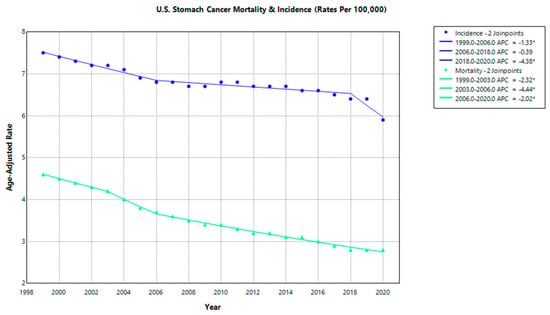
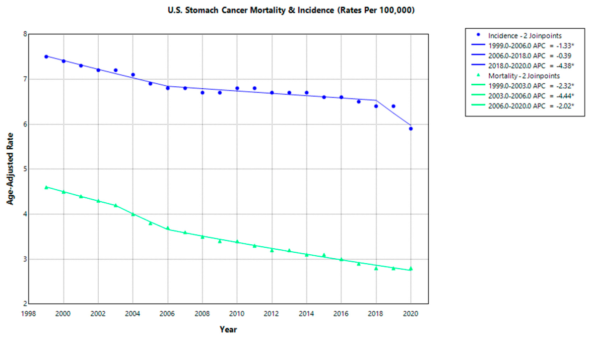
Stomach cancer mortality and incidence data for 1999–2020 at the national level were obtained from the Centers for Disease Control and Prevention [13,14], which compiles cancer statistics through the National Program of Cancer Registries (NPCR) and the Surveillance, Epidemiology, and End Results (SEER) Program. There was a lack of incidence data at the county level, which limited the feasibility of detailed spatial analyses. Thus, incidence estimates were evaluated primarily at the national level, as illustrated in Figure 1, where U.S. stomach cancer incidence rates reported by the CDC are shown in blue and mortality in green.

Figure 1. United States stomach cancer incidence (blue) and mortality (green) rates from 1999 to 2020. Significant changes in slope are indicated as Joinpoints in the legend. An asterisk (*) indicates that the annual percent change (APC) is statistically significantly different from zero (p < 0.05).

County-level mortality data for stomach cancer from 2010–2019 were obtained from the Institute for Health Metrics and Evaluation [15], which generates comprehensive mortality estimates using vital registration systems and additional health data sources. The data were gathered for the 10-year period on 3109 counties, giving this study a sample size of 31,090.

Covariate data for the years 2010–2019 were assembled from multiple sources. Diabetes count data were obtained from IHME [16]. Physical activity, percent unemployed, percent obese, violent crime rate, and percent smokers were derived from the County Health Rankings & Roadmaps (CHR&R), a program of the University of Wisconsin Population Health Institute [17], which provides county-level measures of health outcomes, health behaviors, and social determinants of health. Percent age 45 and over, percent male, percent Black, and county population were obtained from the U.S. Census Bureau American Community Survey [18,19]. Population density was calculated by dividing county population by county land area in square miles obtained from the U.S. Census Bureau Gazetteer Files [20].

The analysis was conducted in two stages. In the first stage, SaTScan™ (version 10.3.2; Information Management Services Inc., Calverton, MD, USA) [21] was used to perform both purely spatial and space–time analyses, including retrospective and prospective scans, under a discrete Poisson model. These methods identified statistically significant geographic clusters based on the likelihood ratio of the scan statistic applied to stomach cancer mortality counts. The resulting spatial and spatiotemporal outputs were then imported into ArcGIS Pro (version 3.6; Esri, Redlands, CA, USA) [22] to generate choropleth maps of counties across the conterminous United States, illustrating variation in stomach cancer mortality rates.

In the second stage, a negative binomial regression model [23] was fitted to account for the effects of explanatory variables on stomach cancer mortality counts. Predicted values from the model were compared with observed mortality counts to assess which clusters persisted after adjustment [24]. This comparison allowed for the identification of clusters that were explained or not explained by the included covariates, and the results were visualized using a three-color map to distinguish between these outcomes.

SaTScan™ [21] is an epidemiological software tool used to detect spatial and spatiotemporal clusters in geographic data. It operates by scanning a study region with circular or elliptical windows that move systematically across space (and time, when applicable). For each scanning window, the observed number of cases is compared to the expected number under a discrete Poisson model, allowing for the identification of areas with unusually high counts relative to the rest of the study region. Clusters are identified by maximizing a likelihood ratio function across all possible window locations and sizes. The most likely cluster (Cluster 1) is the region with the highest likelihood ratio and is the least likely to have occurred by chance. Additional clusters (e.g., Cluster 2, Cluster 3, etc.) are identified sequentially, ensuring that each cluster is geographically distinct and statistically independent of previously detected clusters.

This purely spatial scanning framework extends naturally to space–time analyses by incorporating a temporal dimension into the moving window. In this study, spatial clusters were defined using windows that included up to 25% of the population at risk, while space–time clusters were allowed to span up to 50% of the study period, according to the SaTScan guidelines [25]. A minimum relative risk threshold of 1.0 and a significance level of p < 0.05 were applied, restricting detection to clusters with elevated and statistically significant risk compared to the remainder of the United States. The default number (999) of Monte Carlo replications was used for both the spatial and space–time analysis [25].

The Statistical Analysis System (version 9.4, Maintenance Release 8; SAS Institute Inc., Cary, NC, USA) [26] was used for data preprocessing, model construction, and statistical analysis. A negative binomial regression model [23] was employed to analyze the count-based mortality data using maximum likelihood estimation. This model is an extension of the Poisson framework and is commonly derived from a Poisson–gamma mixture, allowing it to accommodate overdispersion in count data [27].

Unlike the standard Poisson model, which assumes equality of the mean and variance, the negative binomial model incorporates an additional dispersion parameter, making it more appropriate when this assumption is violated [24]. The stomach cancer mortality data in this study exhibited overdispersion, supporting the use of a negative binomial specification. This approach enabled the assessment of covariate effects, with statistical significance evaluated using Wald Chi-Square statistics and corresponding p-values.

The fitted model produced predicted mortality counts, which were subsequently used as input in SaTScan™ to perform covariate-adjusted cluster analyses. These results were then visualized using a three-color mapping scheme to illustrate the extent to which identified clusters were explained by the included covariates.

Missing county-level mortality and covariate values were imputed using state-level mean imputation. Specifically, when a value was unavailable for a county, the missing value was replaced with the mean of that covariate calculated from counties within the same state for which data were available. This approach preserved all counties in the analysis while using geographically relevant information for the imputed value.

No counties were excluded solely on the basis of extreme mortality counts or rates. Because unusually high mortality values may represent meaningful geographic variation rather than erroneous observations, such observations were retained for spatial and regression analyses.

4. Results

4.1. Purely Spatial Analysis

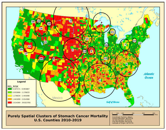
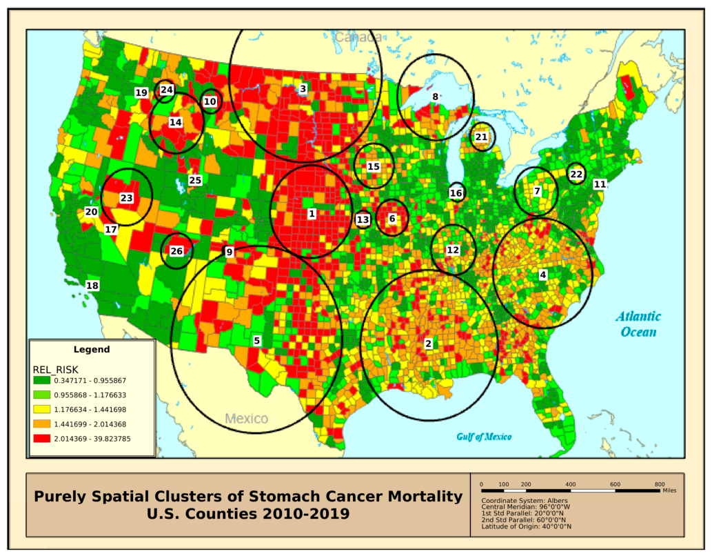
A purely spatial Poisson analysis was conducted using SaTScan™, identifying 26 statistically significant clusters (p < 0.05), as illustrated in Figure 2. These clusters represent regions where stomach cancer mortality rates are disproportionately higher than the national baseline, defined by a relative risk of 1. For example, counties shaded in orange in Figure 2 exhibit relative risks ranging from 1.44 to 2.01, indicating mortality rates up to twice that of the broader study area. Similarly, counties shown in red reflect relative risks at least double the baseline. The clusters are ranked according to the likelihood ratio derived from the spatial scan statistic [28], with Figure 2 displaying the 26 clusters with the highest likelihood ratios.

Figure 2. The 26 purely spatial clusters of stomach cancer mortality for 2010–2019 based on the likelihood ratio of the purely spatial statistic (p < 0.05). The population value is the total population risk within the cluster, summed across all spatial locations in the cluster. Cluster numbers identify individual spatial clusters detected by SaTScan, ranked according to their statistical significance, with Cluster 1 representing the most likely cluster and subsequent numbers representing secondary clusters in descending order of their likelihood ratio statistics.

Table 1 summarizes key characteristics of each cluster, including the number of counties and total population encompassed. Notably, clusters such as 17, 18, 20, and 25 consist of a single county and clusters 9, 10, 19, 24, 26, and 13 consist of fewer than 10 counties, highlighting localized areas of elevated concern. Extremely high relative risks observed in clusters with small populations (e.g., Cluster 7 and Cluster 15) should be interpreted with caution, as they may be influenced by statistical instability or small-number effects.

Table 1. Purely spatial clusters calculated with county-level stomach mortality counts and the population of each county using the discrete scan statistic with Poisson distribution. The clusters are overlaid onto a choropleth map of the rates of stomach cancer mortality in each county. The 10 clusters with the highest likelihood ratios are labeled.

Cluster Number	Counties	Population	Relative Risk
9	2	1502	24.45
17	1	808	22.73
20	1	1122	16.35
25	1	2037	9.01
10	4	11,707	6.28
19	2	6236	5.89
24	3	16,648	3.31
26	3	19,362	2.85
13	9	61,058	2.71
1	127	1,048,633	2.51

4.2. Retrospective Space–Time Analysis

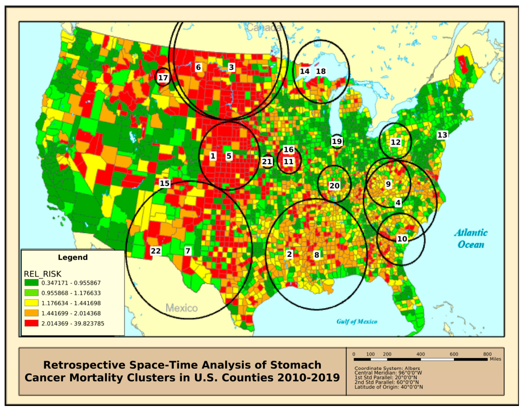
A retrospective space–time analysis was performed to examine how stomach cancer mortality clusters changed over time from 2010 to 2019. Retrospective analysis focuses on previously observed events to establish baseline patterns across both space and time [29]. This allows for identification of specific periods when certain regions experienced unusually high mortality rates.

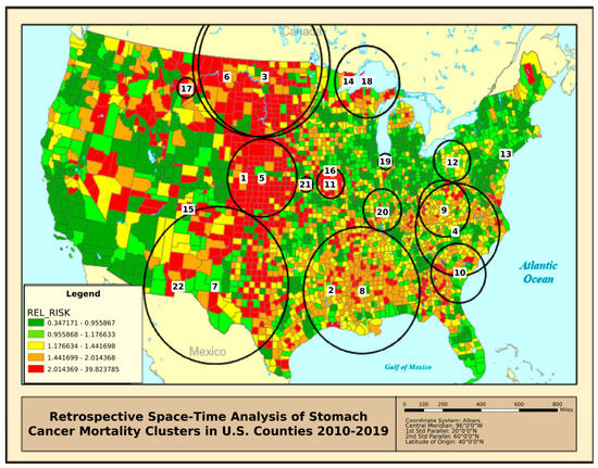
Figure 3 displays the space–time clusters using the same geographic layout as the purely spatial analysis, with the addition of time intervals for each cluster. Table 2 provides details for the most significant clusters, including their size (number of counties), population, relative risk, and the years during which they were active.

Figure 3. Retrospective space–time clusters calculated using the discrete scan statistic with Poisson distribution. The clusters are overlaid onto a choropleth map of the rates of stomach cancer mortality in each county. The 22 clusters with the highest likelihood-ratios are labeled. Cluster numbers are assigned in the same way as those in Figure 2.

Table 2. The significant highest relative risk retrospective space–time clusters of stomach cancer mortality for 2010–2019 based on the likelihood-ratio of the retrospective space–time scan statistic (p < 0.05).

Cluster Number	Counties	Population	Relative Risk	Years
15	2	1502	24.59	2014–2018
17	5	10,489	8.84	2016–2018
21	9	61,058	2.73	2015–2019
1	127	1,048,633	2.51	2013–2017
5	127	1,048,633	2.50	2010–2011
11	36	371,620	1.97	2014–2018
16	36	371,620	1.97	2010–2012
6	137	169,667	1.91	2016–2018
3	149	1,976,684	1.88	2010–2014
14	34	693,204	1.55	2015–2019

The results show that many clusters occur either early or late in the study period. Early clusters may reflect long-standing high-risk areas that were already present before 2010, while later clusters suggest regions where mortality risk has increased more recently. Some clusters also show very high relative risks over short time spans, indicating concentrated spikes in mortality.

By combining spatial and temporal information, this analysis offers deeper insight into how stomach cancer mortality evolves. These findings can also support future prospective modeling efforts by identifying when and where elevated risks are most likely to occur.

4.3. Prospective Space–Time Analysis

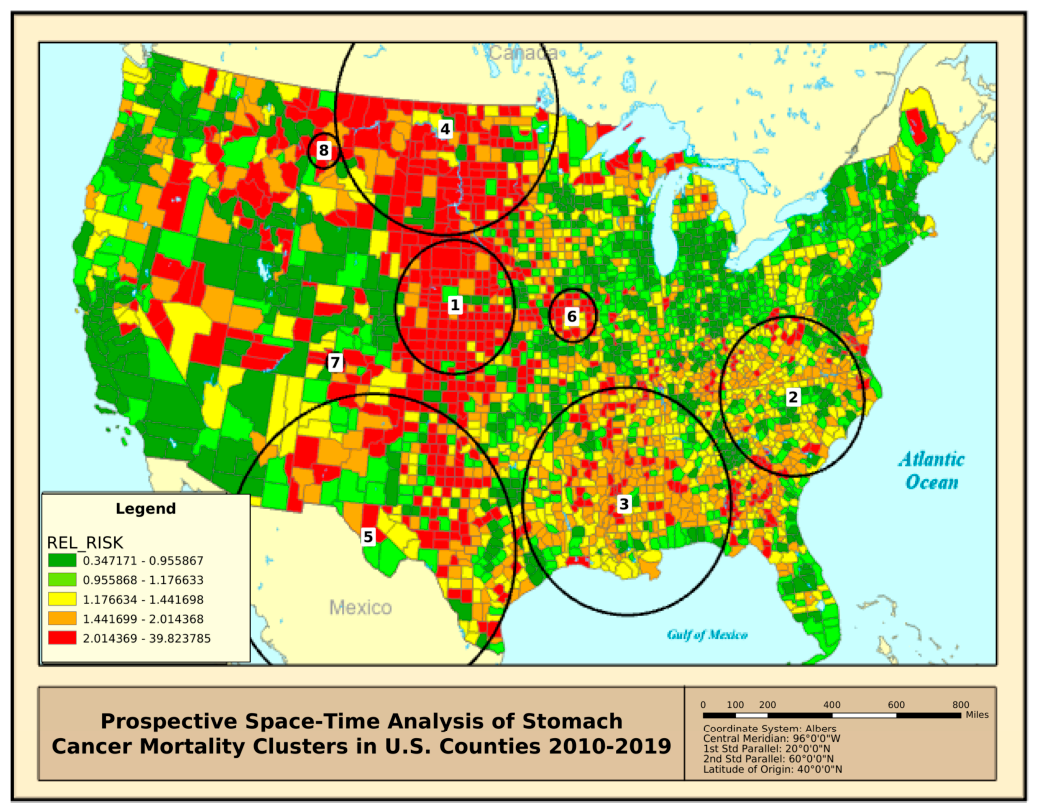
A prospective space–time analysis was performed to detect emerging patterns of stomach cancer mortality using forward-looking methods [30]. This approach establishes a baseline from earlier years and evaluates more recent data to identify clusters that are currently active or increasing in significance. Prospective analysis is commonly used for surveillance and prediction of future high-risk areas.

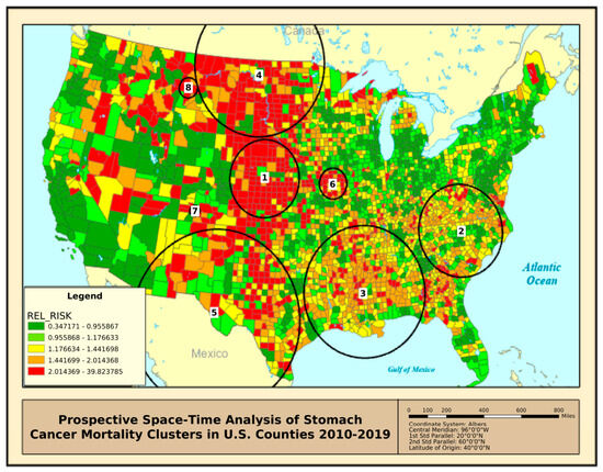
Figure 4 displays the identified clusters, and Table 3 provides details on their size, population, relative risk, and time period. The majority of the clusters are concentrated in the years 2018–2019, suggesting that they represent current hotspots of elevated mortality.

Figure 4. Prospective space–time clusters calculated using the discrete scan statistic with Poisson distribution. The clusters are overlaid onto a choropleth map of the rates of stomach cancer mortality in each county. The clusters with the highest likelihood-ratios are labeled. Clusters numbers are assigned in the same way as Figure 2 and Figure 3.

Table 3. The significant highest relative risk prospective space–time clusters of stomach cancer mortality for 2010–2019 based on the likelihood-ratio of the prospective space–time scan statistic (p < 0.05).

Cluster Number	Counties	Population	Relative Risk	Years
7	3	2221	24.56	2018–2019
8	5	10,489	8.83	2018–2019
1	123	992,730	2.56	2018–2019
6	36	371,620	1.97	2018–2019
4	137	1,649,667	1.96	2018–2019
2	367	23,202,989	1.28	2018–2019
3	414	23,755,870	1.23	2018–2019
5	218	16,285,943	1.13	2018–2019

Some clusters show very high relative risks over short time periods. In particular, Cluster 7 (relative risk = 24.56) involves a small number of counties and population, indicating a sharp and localized increase in mortality. Clusters identified consistently across purely spatial, retrospective, and prospective analyses provide the strongest evidence of persistent geographic disparities in stomach cancer mortality.

These findings highlight regions where stomach cancer mortality is not only historically elevated but continues to be a current concern. As such, the prospective analysis provides valuable information for identifying areas that may require immediate attention and ongoing monitoring.

4.4. Covariate Analysis

The negative binomial regression model with covariates listed in Table 4 was used to adjust stomach cancer mortality counts for spatial analysis. Table 4 shows the parameter estimates for predicting stomach cancer mortality counts along with the associated test statistics. Positive parameter estimates reflect a direct relationship in which a one-unit increase in the covariate corresponds to an increase in the logarithm of the expected stomach cancer mortality rate equal to the estimated parameter value. Positive parameter estimates were observed for all ten of the covariates in Table 4 and a Pearson Chi-Square (via SAS) value of 0.8804 ≈ 1, meaning our model has achieved a high goodness of fit.

Table 4. Analysis of maximum likelihood parameter estimates from negative binomial regression.

Parameter	DF	Estimate	SE	Lower 95% Limit	Upper 95% Limit	Wald χ2	Pr > ChiSq
Intercept	1	−12.5178	0.1010	−12.7158	−12.3197	15,348.70	<0.0001
% of Population Age 45 and Over	1	0.0207	0.0004	0.0189	0.0215	2307.87	<0.0001
% of Population Physically Inactive	1	0.0109	0.004	0.0102	0.0116	891.75	<0.0001
% of Unemployed Population	1	0.0175	0.0007	0.0161	0.0189	623.33	<0.0001
% of Male Population	1	2.2295	0.1975	1.8423	2.6167	127.37	<0.0001
% of Obese Population	1	0.0075	0.0007	0.0061	0.0088	112.25	<0.0001
Violent Crime Rate	1	17.1943	2.1023	13.0738	21.3148	66.89	<0.0001
Population per Square Mile	1	0.0010	0.0001	0.0007	0.0012	46.95	<0.0001
% of Diabetic Population	1	0.6908	0.1131	0.4692	0.9124	37.33	<0.0001
% of Smokers	1	0.0038	0.0007	0.0023	0.0052	25.76	<0.0001
% of Black Population	1	0.0007	0.0002	0.0003	0.0010	14.29	0.0002
Dispersion	1	0.0064	0.0004	0.0055	0.0073	-	-

DF = degrees of freedom; SE = standard error; Wald χ² = Wald chi-square statistic; Pr > ChiSq = probability associated with the chi-square test (p-value).

Each of the covariates used was significant at the p < 0.05 level. The parameters are listed in decreasing order using Wald’s Chi-Square statistic, which considers the effect of the covariate when it is added last to the model. The percent of the population over the age of 45 in a county had the largest Chi-Square value of 2307.87, implying it has the largest effect on stomach cancer mortality rates when the other covariates are held constant in the model. Counties with a high death rate caused by percentage of people physically inactive was the second-most important covariate with a Chi-Square value of 891.75. The percentage of unemployed people was the third-most important covariate in the model with a Chi-Square value of 623.33.

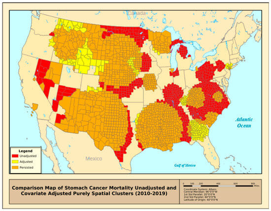
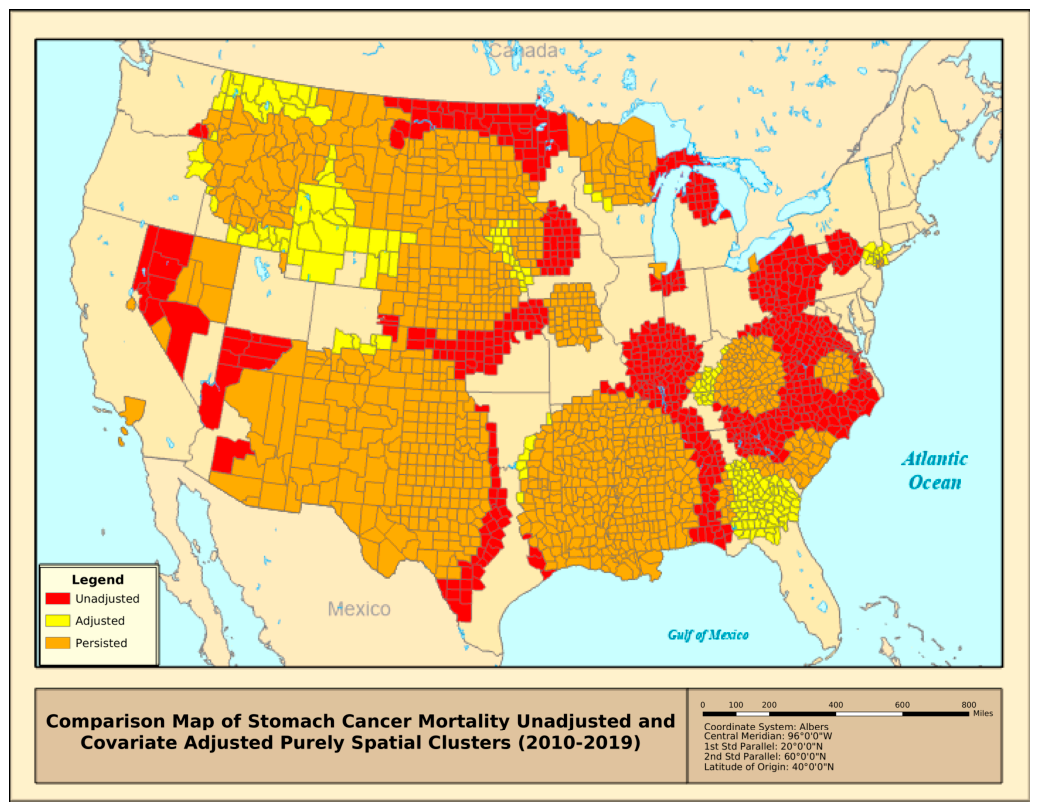
A comparison map of locations in the original unadjusted spatial clusters and locations in covariate-adjusted spatial clusters is shown in Figure 5. Red areas represent those which appeared only in the original significant spatial clusters. Yellow areas are clusters which appeared only after adjusting for the covariates. Orange areas are those which appeared in clusters both before and after covariate adjustment.

Figure 5. A three-color map of locations in the original unadjusted spatial clusters and locations in covariate-adjusted spatial clusters.

5. Discussion

This surveillance study provides a spatiotemporal analysis of stomach cancer mortality in the United States at the county level, in addition to identifying which risk factors are the strongest predictors of stomach cancer mortality for the period 2010–2019. Stomach cancer mortality rates differ significantly across the United States, and the analysis identifies clusters with the highest likelihood ratio of scan statistic of mortality. The spatial clusters expose areas where stomach cancer mortality count is disproportionately high compared to the rest of the country, while spatiotemporal clusters further reveal times of historically high mortality and emerging clusters toward the end of the study period.

In Table 1 and Table 2, it is highlighted that the cluster with the highest likelihood ratio of the scan statistic was centered (clusters are defined by a scanning window centered on a county but include multiple surrounding counties within the optimal radius) in Frontier County, Nebraska. The relative risk of this cluster was more than 2.5 times the baseline mortality risk across the study area, as determined by the spatial scan statistic. The highest relative risk counties were San Juan and Ouray counties in Colorado with relative risk over 24 times the baseline mortality risk. The largest clusters with respect to area and population were identified covering a broad portion of central Southwestern and Northwestern United States. The relative risk of these widely spread clusters was lower than that of isolated clusters, but it provides valuable insights into regional disparities in stomach cancer mortality. Correct interpretation of these findings is necessary, as smaller clusters with extremely high relative risk may be affected by localized factors such as limited healthcare access, H. pylori infection rate or environmental carcinogen exposure. For example, the concentration of clusters in the southern United States may reflect higher prevalence of known risk factors such as socioeconomic disadvantage, reduced healthcare access, dietary patterns, and higher rates of H. pylori infection.

Table 4 presents the results from the negative binomial regression model, which assesses the influence of different covariates on stomach cancer mortality. The three-color map clarifies the spatial distribution of mortality clusters after adjusting for these covariates, highlighting persistent clusters (areas with high mortality rates unexplained by the selected factors) in Arizona, New Mexico, Colorado, Texas, Louisiana, Mississippi, Missouri, Nebraska, the Dakotas, and Wisconsin (Figure 5), among others. These persistent clusters (shown in orange) suggest the presence of additional unaccounted-for risk factors, such as genetic predisposition, unmeasured environmental exposures, disparities in healthcare access or additional potential covariates not listed here. Meanwhile, regions where high mortality rates were largely explained by the selected covariates are shown in red, indicating that known risk factors such as obesity, physical inactivity, and socioeconomic variables adequately describe mortality patterns in those locations.

The key findings from this study are two-fold. The first key finding is the actual clusters of stomach cancer mortality themselves, while the second key finding is the persistent clusters, those colored orange in Figure 5, of stomach cancer mortality. While this study was not broken down by population groups as was the 2023 study discussed in the literature review, at an aggregate level, multiple clusters affirm placements of the elevated stomach cancer mortality rates found in the analysis by racial-ethnic groups. Additionally, the elevated mortality counties in the Southern United States noted by Ma and colleagues appear in a large persistent cluster in Figure 5. With significant spatial overlap found between this study and the 2022 and 2023 research, this study takes the further step of investigating whether the clusters can be explained with the selected covariates. Figure 5 shows that the model and selected covariates were able to explain some of the identified clusters in this study, particularly in the Eastern and Northeastern United States. However, the three large persistent clusters from Figure 5 that overlap between this study and other research are largely unexplained, which presents a ripe opportunity for further investigation.

This study has several limitations that should be considered when interpreting the results. First, the analysis was conducted at the county level, which may introduce ecological bias, as relationships observed at the aggregate level may not necessarily reflect individual-level risk factors. Second, some important variables, such as H. pylori infection rates, dietary patterns, and environmental exposures, were not directly included due to data limitations, potentially leaving residual confounding in the model. Third, the use of modeled mortality estimates from IHME may introduce uncertainty compared to directly observed vital statistics, particularly in counties with small populations. Additionally, clusters identified with very small populations may exhibit inflated relative risks due to statistical instability. Finally, the spatial scan statistic assumes circular cluster shapes and may not fully capture irregular geographic patterns of disease distribution. Despite these limitations, the study provides valuable insights into spatial and temporal patterns of stomach cancer mortality across the conterminous United States.

6. Conclusions

The analysis identified significant associations between stomach cancer mortality and demographic, behavioral, and socioeconomic factors. Key predictors of high mortality included age over 45, unemployment rate, obesity, percent physically inactive, and being male.

This work does not demonstrate causal relationships between individual covariates and stomach cancer mortality but points to strong associations that call for further investigation. Future research should focus on incorporating individual-level data, additional environmental variables, and improved access measures to better explain unexplained high-risk clusters, particularly the three common clusters noted between this study and the 2023 study [11]. Further research could also provide the potential to drill into the larger regional clusters of stomach cancer mortality and investigate whether sub-clusters exist and if they can be explained or not, or to use updated SaTScan parameters, e.g., p < 0.01, for greater precision in results. In addition, incorporating genetic data, environmental exposure assessments, and access to stomach cancer screening and treatment could provide a more comprehensive understanding of mortality patterns in the United States. Tackling disparities in healthcare access and increasing preventive measures in high-risk regions could be essential steps in reducing stomach cancer mortality.

References

- Ilić, M.; Ilić, I. Epidemiology of stomach cancer. World J. Gastroenterol. 2022, 28, 1187–1203. [Google Scholar] [CrossRef] [Scilit] [PubMed]
- National Cancer Institute. Cancer Stat Facts: Stomach Cancer. Surveillance, Epidemiology, and End Results (SEER) Program; National Cancer Institute: Singapore, 2024. Available online: https://seer.cancer.gov/statfacts/html/stomach.html (accessed on 19 March 2026).
- Cover, T.L.; Blaser, M.J. Helicobacter pylori in health and disease. Gastroenterology 2009, 136, 1863–1873. [Google Scholar] [CrossRef] [Scilit] [PubMed]
- Wu, B.; Yang, D.; Yang, S.; Zhang, G. Dietary salt intake and gastric cancer risk: A systematic review and meta-analysis. Front. Nutr. 2021, 8, 801228. [Google Scholar] [CrossRef] [Scilit] [PubMed]
- Lee, K.W.; Woo, H.D.; Cho, M.J.; Park, J.K.; Kim, S.S. Identification and epidemiological evaluation of gastric cancer risk factors: Based on a field synopsis and meta-analysis in Chinese population. Sci. Rep. 2021, 11, 18437. [Google Scholar]
- Maddineni, G.; Xie, J.J.; Brahmbhatt, B.; Mutha, P. Diet and carcinogenesis of gastric cancer. Curr. Opin. Gastroenterol. 2022, 38, 588–591. [Google Scholar] [CrossRef] [Scilit] [PubMed]
- Trédaniel, J.; Boffetta, P.; Buiatti, E.; Saracci, R.; Hirsch, A. Tobacco smoking and gastric cancer: Review and meta-analysis. Int. J. Cancer 1997, 72, 565–573. [Google Scholar] [CrossRef] [Scilit]
- Na, H.K.; Lee, J.Y. Molecular basis of alcohol-related gastric and colon cancer. Int. J. Mol. Sci. 2017, 18, 1116. [Google Scholar] [CrossRef] [Scilit] [PubMed]
- Azizi, N.; Zangiabadian, M.; Seifi, G.; Davari, A.; Yekekhani, E.; Safavi-Naini, S.A.A.; Berger, N.A.; Nasiri, M.J.; Sohrabi, M.R. Gastric cancer risk in association with underweight, overweight, and obesity: A systematic review and meta-analysis. Cancers 2023, 15, 2778. [Google Scholar] [CrossRef] [Scilit] [PubMed]
- Jo, H.H.; Kim, N.; Jang, J.; Choi, Y.; Lee, J.W. Differences in the effect of physical activity on the prevention of gastric cancer according to sex. J. Gastric Cancer 2025, 25, 343–355. [Google Scholar] [CrossRef] [Scilit] [PubMed]
- Kendrick, P.; Kelly, Y.O.; Baumann, M.M.; Compton, K.; Blacker, B.F.; Daoud, F.; Li, Z.; Mouhanna, F.; Nassereldine, H.; Schmidt, C.; et al. The burden of stomach cancer mortality by county, race, and ethnicity in the USA, 2000–2019: A systematic analysis of health disparities. Lancet Reg. Health Am. 2023, 24, 100547. [Google Scholar] [CrossRef] [Scilit] [PubMed]
- Ma, C.; Congly, S.E.; Chyou, D.E.; Ross-Driscoll, K.; Forbes, N.; Tsang, E.S.; Sussman, D.A.; Goldberg, D.S. Factors Associated with Geographic Disparities in Gastrointestinal Cancer Mortality in the United States. Gastroenterology 2022, 163, 437–448.e1. [Google Scholar] [CrossRef] [Scilit] [PubMed]
- Centers for Disease Control and Prevention. United States and Puerto Rico Cancer Statistics, 1999–2022 Incidence; CDC WONDER Online Database; Centers for Disease Control and Prevention: Atlanta, GA, USA, 2024. Available online: https://wonder.cdc.gov/cancer-v2022.html (accessed on 1 July 2026).
- Centers for Disease Control and Prevention. United States and Puerto Rico Cancer Statistics, 1999–2021 Mortality; CDC WONDER Online Database; Centers for Disease Control and Prevention: Atlanta, GA, USA, 2023. Available online: https://wonder.cdc.gov/cancermir-v2021.html (accessed on 1 July 2026).
- Institute for Health Metrics and Evaluation (IHME). United States Stomach Cancer Mortality by County, Race, and Ethnicity, 2000–2019; Institute for Health Metrics and Evaluation: Seattle, WA, USA, 2023; Available online: https://ghdx.healthdata.org/record/ihme-data/united-states-stomach-cancer-mortality-by-county-race-ethnicity-2000-2019 (accessed on 1 July 2026).
- Institute for Health Metrics and Evaluation (IHME). United States Diabetes Prevalence by County, Race, and Ethnicity, 2000–2019; Institute for Health Metrics and Evaluation: Seattle, WA, USA, 2022; Available online: https://ghdx.healthdata.org/record/ihme-data/us-diabetes-county-race-ethnicity-2000-2019 (accessed on 1 July 2026).
- University of Wisconsin Population Health Institute. County Health Rankings & Roadmaps: 2019 County Health Rankings National Data; University of Wisconsin: Madison, WI, USA, 2019. Available online: https://www.countyhealthrankings.org/health-data/methodology-and-sources/data-documentation/national-data-documentation-2010-2023 (accessed on 1 July 2026).
- U.S. Census Bureau. American Community Survey 5-Year Estimates, 2019; Table S0101: Age and Sex.; U.S. Department of Commerce: Washington, DC, USA, 2020. Available online: https://data.census.gov/table/ACSST5Y2019.S0101?g=010XX00US%240500000 (accessed on 1 July 2026).
- U.S. Census Bureau. American Community Survey 5-Year Estimates, 2019; Table DP05: ACS Demographic and Housing Estimates; U.S. Department of Commerce: Washington, DC, USA, 2020. Available online: https://data.census.gov/table/ACSDP5Y2019.DP05?g=010XX00US%240500000 (accessed on 1 July 2026).
- U.S. Census Bureau. 2019 U.S. Gazetteer Files: Counties; U.S. Department of Commerce: Washington, DC, USA, 2019. Available online: https://www.census.gov/geographies/reference-files/time-series/geo/gazetteer-files.2019.html (accessed on 1 July 2026).
- Kulldorff, M. SaTScanTM Statistical Software, Version 10.3.2 (64-bit); Information Management Services, Inc.: Silver Spring, MD, USA, 2025. Available online: https://www.satscan.org/download.html (accessed on 19 March 2026).
- ESRI. ArcGIS Pro, Version 3.6; Environmental Systems Research Institute: Redlands, CA, USA, 2023. Available online: https://www.esri.com/en-us/arcgis/products/arcgis-pro/ (accessed on 19 March 2026).
- Hilbe, J.M. Negative Binomial Regression; Cambridge University Press: Cambridge, UK, 2007. [Google Scholar] [CrossRef] [Scilit]
- Hilbe, J.M. Modeling Count Data; Cambridge University Press: Cambridge, UK, 2014. [Google Scholar] [CrossRef] [Scilit]
- Kulldorff, M. SaTScan User Guide (Version 10.1); Information Management Services, Inc.: Silver Spring, MD, USA, 2025; Available online: https://www.satscan.org/cgi-bin/satscan/register.pl/SaTScan_Users_Guide.pdf?todo=process_userguide_download (accessed on 19 March 2026).
- SAS Software, Version 9.4 of the SAS System for Windows; SAS Institute Inc.: Cary, NC, USA, 2021.
- Zwilling, M. Negative binomial regression. Math. J. 2013, 15, 1–18. [Google Scholar] [CrossRef] [Scilit]
- Kulldorff, M. A spatial scan statistic. Commun. Stat. Theory Methods 1997, 26, 1481–1496. [Google Scholar] [CrossRef] [Scilit]
- Kulldorff, M.; Athas, W.F.; Feurer, E.J.; Miller, B.A.; Key, C.R. Evaluating cluster alarms: A space-time scan statistic and brain cancer in Los Alamos. Am. J. Public Health 1998, 88, 1377–1380. [Google Scholar] [CrossRef] [Scilit] [PubMed]
- Kulldorff, M. Prospective time-periodic geographical disease surveillance using a scan statistic. J. R. Stat. Soc. Ser. A Stat. Soc. 2001, 164, 61–72. [Google Scholar] [CrossRef] [Scilit]
Disclaimer/Publisher’s Note: The statements, opinions and data contained in all publications are solely those of the individual author(s) and contributor(s) and not of MDPI and/or the editor(s). MDPI and/or the editor(s) disclaim responsibility for any injury to people or property resulting from any ideas, methods, instructions or products referred to in the content. |
© 2026 by the authors. Licensee MDPI, Basel, Switzerland. This article is an open access article distributed under the terms and conditions of the Creative Commons Attribution (CC BY) license.