


Abstract
Accurate characterization and compensation of Earth–Moon reference-clock differences are important for cislunar positioning, navigation, and timing (PNT) architectures. This study develops an integrated analytical framework that connects modeled Earth–Moon timing differences, compensation residuals, and position-domain sensitivity. A first-order weak-field and slow-motion model is used to generate an idealized Earth–Moon reference-clock difference series, which accumulates to approximately 20.48 ms over 365.25 days under the adopted assumptions. Compensation performance is evaluated using chronological training and held-out evaluation for autonomous forecast models, together with full-interval correction-product reconstruction. Because the reference and validation sequences are generated within the same analytical framework, the forecast results represent model-consistent internal validation rather than independent empirical evidence of real Earth–Moon clock predictability. The resulting timing residuals are propagated through a linearized four-state least-squares estimator that jointly solves for three-dimensional position and receiver-clock range bias. The analysis shows that the position-domain effect of a timing residual depends not only on its magnitude, but also on its source-dependent structure, observation geometry, estimator conditioning, and non-timing error floor. The inferred timing thresholds are therefore conditional architecture-level sensitivity results for the adopted estimator, controlled geometries, and stochastic error model, rather than operational requirements for a specific lunar navigation constellation. The framework provides a transparent baseline for future studies incorporating higher-order clock modeling, dynamic orbit determination, sequential estimation, time-varying visibility, correlated measurement errors, inter-satellite measurements, and independent Earth–Moon timing data.
1. Introduction
Renewed scientific and engineering activity in the Earth–Moon system has increased interest in positioning, navigation, and timing (PNT) architectures for users beyond the immediate vicinity of Earth. Candidate lunar and cislunar concepts may combine Earth-based infrastructure, lunar-orbiting sources, surface assets, and Earth–Moon or inter-satellite communication links [1,2,3,4]. A consistent lunar reference frame and an associated time reference are important components of such architectures [5,6]. Time is involved not only in clock synchronization, but also in signal transmission, observation time tagging, orbit determination, and pseudorange formation. Consequently, the relationship between terrestrial and lunar time references has implications for both relativistic reference-time transformations and navigation measurement formation [5,7,8,9,10].
Clocks associated with terrestrial and lunar reference environments do not accumulate proper time at identical rates. In the weak-field and slow-motion approximation, the rate of a clock relative to a selected coordinate time is determined primarily by the gravitational potential and the clock’s kinematic state [7,9,11]. Idealized Earth- and Moon-associated clocks therefore exhibit both different mean rates and time-dependent rate variations. The leading contributions arise from their distinct gravitational and kinematic environments, while external-body potentials, orbital motion, rotational motion, non-spherical gravity, and higher-order relativistic effects may provide additional terms [12,13,14]. Although the corresponding fractional-frequency differences are small, their integrated effect can become significant over the time intervals relevant to cislunar navigation and time transfer.
A consistent treatment of these effects requires clearly defined reference systems and coordinate time scales. The International Astronomical Union (IAU) framework provides the basis for barycentric and geocentric relativistic reference systems and their associated time transformations [7,8,9], while the International Earth Rotation and Reference Systems Service (IERS) conventions specify the practical realization of terrestrial time scales and related reference quantities [10]. Recent work has extended these foundations to Earth–Moon transformations, lunar reference systems and frames, and possible realizations of a lunicentric coordinate time [5,6,15]. Turyshev et al. derived transformations among barycentric, geocentric, and lunicentric time coordinates and identified secular and periodic components of the terrestrial–lunar time difference [15]. Fienga et al. discussed lunar reference systems and possible implementations of a lunicentric time scale for orbiting and surface-based clocks [5]. Related studies have also considered the generation and dissemination of numerical lunar time-ephemeris correction products [16,17].
These developments motivate a distinction between the physical relation among reference times and the residual remaining after that relation has been modeled, predicted, or disseminated as a correction. The former concerns the definition and transformation of reference times. The latter directly affects observation formation and the behavior of navigation estimators. This study focuses on the second connection. It uses an idealized Earth–Moon reference-clock model as a controlled input and examines how its residual errors propagate into a simplified cislunar PNT solution. It does not attempt to define a formal lunar coordinate time or to reproduce a complete Geocentric Coordinate Time (TCG)–Lunicentric Coordinate Time (TCL) or Terrestrial Time (TT)–Lunar Time (TL) transformation.
Relativistic clock modeling and time-frequency transfer have been studied extensively in terrestrial and solar-system applications [12,13,14]. In satellite navigation, clock errors are commonly represented as range-equivalent observation errors, while receiver clock bias is estimated jointly with user position [18,19,20,21]. These estimation principles provide the basis for analyzing the timing-to-position connection in a cislunar setting. However, they also show why a clock difference cannot be converted uniquely into a three-dimensional position error.
Multiplying a timing offset by the speed of light gives the associated one-way range-equivalent quantity,
which expresses the timing effect in observation-domain units. This quantity is not itself a position error. For observations from multiple sources, the timing residual may be decomposed as
where is common to all observations and is source dependent. To first order, a strictly common component has the same observation signature as a receiver-clock range bias and can therefore be absorbed by the estimated clock state when that state is included consistently. A source-dependent component is not generally parallel to the receiver-clock column of the design matrix and can project into the position-sensitive observation subspace. Its effect depends on the source geometry, observation weighting, estimator conditioning, and non-timing error budget [18,19,21]. Thus, timing residual magnitude alone does not determine position degradation.
The assessment of timing compensation introduces a second information distinction. A model fitted to past data and extrapolated to later epochs constitutes a forecast. In contrast, a tabulated correction product with correction nodes available throughout the evaluation interval supports interpolation or reconstruction. These cases do not provide the estimator with the same information and should not be treated as equivalent forms of validation. A continuously available product may achieve a small reconstruction residual, while its performance during update loss depends on the local holdover model and its ability to represent the time-varying clock rate. Chronological validation, correction cadence, update continuity, and outage behavior must therefore be assessed separately. This distinction is particularly important when both the reference and validation sequences are generated from the same analytical model.
A related issue arises when a positioning target is inverted to obtain an allowable timing error. Timing is only one component of the total observation error budget. Orbit and ephemeris uncertainty, source-clock noise, measurement noise, propagation-related residuals, hardware delays, and source geometry can produce a non-timing position-error floor. Once the source-dependent timing contribution becomes small relative to this floor, further timing improvement produces limited reduction in total position error. A specified position target may therefore be unattainable under a given geometry and non-timing error budget, even when the timing residual is reduced toward zero. The resulting allowable timing value is consequently a conditional sensitivity threshold, not a universal clock specification [19,20,21].
The numerical results also depend on the dynamical inputs used to generate the reference series. The DE430/DE431 and DE440/DE441 ephemerides provide successive high-precision frameworks for planetary and lunar state-vector calculations [22,23], while lunar gravity models based on Clementine and GRAIL tracking data provide increasingly detailed representations of the lunar gravitational environment [24,25]. In the present study, DE440s barycentric states provide the position and velocity inputs for an idealized first-order reference-clock calculation. The ephemeris is used as a dynamical input to the numerical experiments; no new ephemeris, complete lunar gravity model, or formal lunar coordinate-time realization is developed.
To trace the connection from modeled clock behavior to PNT sensitivity, the study conducts three linked numerical experiments. Experiment 01 generates a model-defined Earth–Moon reference-clock difference series from DE440s barycentric states using a first-order weak-field and slow-motion proper-time model. The calculation separates the adopted self-gravity, external-gravity, orbital-motion, and equatorial-rotation contributions and characterizes the resulting secular accumulation and time-dependent structure. The series serves as a controlled input for the compensation and navigation analyses.
Experiment 02 evaluates several compensation cases: an uncompensated baseline, a training-only linear-drift model, prescribed harmonic forecast models, and a full-interval tabulated correction product. Chronologically separated training and evaluation intervals are used to distinguish out-of-sample forecasting from reconstruction. Multi-window tests and component-removal analyses examine the behavior of the parametric forecast models, while correction-cadence and update-outage tests characterize the idealized product under different information-delivery conditions. Because the reference and validation sequences are generated within the same analytical framework, the results represent internal, model-consistent validation rather than independent empirical validation of real Earth–Moon clock predictability.
Experiment 03 propagates the compensation residuals through a linearized four-state least-squares PNT estimator that jointly solves for three-dimensional receiver position and receiver clock range bias. The timing residual is separated into common and source-dependent components to examine their different estimator signatures. Controlled GOOD, MODERATE, and POOR source geometries and a parameterized non-timing error budget are then used to evaluate position position root-mean-square error (RMSE) and to invert selected position targets into conditional source-dependent timing-sensitivity thresholds. The geometry analysis is motivated by previous lunar PNT and lunar-augmented navigation studies [1,2,3], but the geometries used here are controlled sensitivity cases rather than representations of Moonlight, LunaNet, or any other proposed operational constellation.
The analysis addresses three questions:
- What secular and time-dependent structures arise from the adopted first-order model of the Earth–Moon reference-clock difference?
- How do training-only forecasts and a tabulated correction product differ in residual accuracy, temporal robustness, cadence sensitivity, and outage behavior under model-consistent validation?
- How do common and source-dependent timing residuals map into a four-state position–clock solution, and how do source geometry and the non-timing error floor constrain the source-dependent timing error associated with a selected position target?
The primary contributions are threefold. First, the study establishes a traceable architecture-level framework connecting a first-order, model-generated Earth–Moon reference-clock difference to compensation residuals and their propagation through a PNT estimator. Second, it evaluates forecast models and a tabulated correction product under explicitly separated information conditions, including chronological hold-out intervals, correction-cadence changes, and product-delivery outages. Third, it demonstrates within a controlled four-state estimator why a scalar range-equivalent timing error does not uniquely determine position degradation, and quantifies how source-dependent residual structure, source geometry, and the non-timing error floor jointly determine conditional timing-sensitivity thresholds.
2. Theoretical Framework
2.1. Relativistic Time-Reference Difference
For a clock moving with coordinate velocity magnitude v in a weak gravitational field, the relation between proper time and a selected coordinate time t can be written, to first order in the weak-field and slow-motion approximation, as
where U denotes the adopted positive gravitational potential, v is the coordinate speed of the clock, and c is the speed of light.
For two reference clocks, denoted by E and L, the differential rate with respect to the same coordinate time is therefore
The potential and velocity terms can be separated according to their physical origin:
with
In the cislunar case, the gravitational contribution may contain the self-potentials of the Earth and Moon as well as potentials generated by external bodies. The kinematic contribution may include the orbital and rotational terms retained by the adopted reference model. The detailed decomposition used in the numerical experiments is introduced in Section 3.1.
The accumulated time-reference difference is evaluated numerically from the sampled rate series:
with
Equation (8) applies the trapezoidal rule to the sampled reference-rate sequence. The initial condition defines the zero point of the numerical comparison. Consequently, describes the relative evolution from the initial epoch, rather than an absolute synchronization offset or an absolute realization of an Earth–Moon coordinate time scale.
The time difference can be expressed as a one-way range-equivalent quantity:
This conversion places the timing difference in the same observation-domain units as a pseudorange error. It is not interpreted as a direct three-dimensional position error because the receiver-clock state is estimated jointly with the position states.
2.2. Observation Model and Error Decomposition
For observed signal sources, the linearized pseudorange observation model is written as
where
contains the three position errors and the receiver-clock range-equivalent error. The design matrix is
where is the unit line-of-sight vector from the receiver to source i.
The observation error is decomposed into timing and non-timing components:
The timing component is further separated into common and source-dependent parts:
where is an -dimensional vector of ones, is the common timing residual, and contains the source-dependent residuals.
The common component has the same value in every observation. Its observation signature is parallel to the receiver-clock column of and can therefore be represented by the receiver-clock state. The differential component has source-dependent values and is not generally parallel to that column. It can consequently produce a position error.
For a weighted least-squares solution, define
where is the observation-weight matrix. The estimated state error caused by an observation perturbation is
Let extract the three position components from the state. The corresponding position error is
For the common timing term,
the position contribution is zero to first order when the receiver-clock state is included, the design matrix is consistent with the observation model, and the weighted system is nonsingular. This follows from
which shows that the common observation perturbation has the same signature as a receiver-clock range bias.
For the differential term,
the position contribution is generally non-zero:
The mapping depends on both the source-dependent timing pattern and the design matrix. It is therefore not determined by the scalar quantity alone.
This decomposition provides the theoretical basis for separating the total compensation residual from the source-dependent timing residual in Experiment 03. It also explains why a one-way range-equivalent timing residual cannot be interpreted directly as a three-dimensional position error.
2.3. Compensation Residuals and Temporal Prediction
Let denote the reference time-difference series and its estimate under compensation model m. The compensation residual is
For a parametric forecast model, the estimate is determined only from a training data set:
Here, denotes the fitting and prediction procedure for model m, is the training interval, and is a later held-out interval.
The validation residual therefore measures out-of-sample prediction under the adopted analytical reference-clock model. Model complexity determines which temporal components can be represented, but increased complexity does not guarantee improved validation performance. A fitted component may describe the training interval accurately while extrapolating poorly beyond that interval.
For a full-interval correction product, the estimate is instead obtained from correction nodes available throughout the evaluation period:
where denotes the selected interpolation or reconstruction operator and denotes the set of correction nodes spanning the evaluation interval.
Equations (24) and (25) represent different information conditions. The former describes prediction without access to future reference values, whereas the latter describes reconstruction while correction information remains available. Their residuals are therefore reported separately in Experiment 02 and are not treated as equivalent measures of autonomous forecasting performance.
The correction-product node spacing introduces a separate interpolation error. If h denotes the node spacing and the correction series is sufficiently smooth, the interpolation residual can be written locally as
For linear interpolation, the leading local error is proportional to and the local curvature of the underlying series:
This relation explains the expected sensitivity to correction cadence over the tested spacing range. It does not describe holdover after future correction updates are interrupted.
For an update outage beginning at , let the last available correction be and let denote the prescribed holdover rate. The holdover estimate is
The corresponding outage residual is
Unlike interpolation, this residual depends on the accumulated mismatch between the actual time-varying rate and the retained holdover rate:
Therefore, outage residuals generally grow with interruption duration and cannot be inferred from the continuously available-product interpolation RMS.
2.4. PNT Error Propagation and Timing-Sensitivity Inversion
Let the source-dependent timing-error covariance be represented as
where is the characteristic source-dependent timing error and describes its normalized source pattern or source-wise correlation structure.
The corresponding pseudorange-error covariance is
Let denote the covariance of the remaining error budget. Under the independent-error assumption used in the primary analysis,
The state-error covariance is then
Let extract the three position components from the state. The three-dimensional position RMS is defined by
The factor contains the influence of source geometry and the source-dependent timing-error structure. The quantity is the position-error floor caused by the non-timing components of the observation error.
For a prescribed position-RMS target , the allowable source-dependent timing error follows from
provided that
If Equation (40) is not satisfied, the target is not attainable by improving timing accuracy alone. Equation (39) gives the analytical threshold for the covariance model. In the numerical analysis, the corresponding threshold is obtained from the forward position-error model and the numerical search procedure described in Section 3.6.
The theoretical result has two limiting behaviors. When the timing term dominates the non-timing floor,
the position RMS is approximately proportional to :
When the timing contribution is small,
the position RMS approaches the non-timing floor:
This transition explains why improving time-reference accuracy does not necessarily improve the final positioning result once the non-timing error floor becomes dominant.
The analytical covariance relation also clarifies the role of geometry. For a fixed source-dependent timing pattern and a fixed non-timing error budget, a poorly conditioned design matrix increases both and the propagated non-timing contribution. Consequently, a timing level that is sufficient under favorable geometry may be insufficient under a near-degenerate geometry.
The covariance formulation describes the statistical propagation of source-dependent timing uncertainty. The deterministic residual analysis used for the compensation cases is obtained by applying the same linear mapping to the realization-specific observation residual:
Thus, the analytical threshold relation and the numerical Monte Carlo results address the same error-propagation chain under complementary representations: the former describes covariance-level sensitivity, while the latter evaluates realization-level position statistics.
2.5. Scope of the Framework
The framework developed in this study is intended for architecture-level sensitivity analysis of the relationship between Earth–Moon reference-clock differences, timing compensation residuals, and cislunar positioning performance. It is not intended to provide a formal realization of a lunar coordinate time, establish operational timing requirements for a specific mission, or predict the performance of a particular lunar navigation constellation.
The time-reference model retains the leading weak-field and slow-motion terms in the adopted proper-time relation. It provides a controlled baseline for examining how modeled timing differences propagate through compensation and PNT analyses. Higher-order relativistic terms, non-spherical and time-varying gravity-field effects, tidal deformation, detailed body orientation, site-specific clock locations, orbit–rotation cross terms, and mission-specific time-transfer procedures are outside the primary model. The resulting reference series is therefore a model-defined analytical input, not an independent empirical realization of the actual Earth–Moon clock difference.
The navigation analysis uses a linearized four-state position–clock model consisting of three position coordinates and one receiver-clock range-equivalent bias. This formulation isolates the observation-space distinction between common and source-dependent timing residuals. It does not represent a complete dynamic orbit-determination or sequential navigation filter. Process-noise tuning, state propagation, dynamic-model errors, measurement editing, cycle slips, and filter-initialization effects are outside the present scope.
The source geometries are controlled configurations rather than time-varying geometries associated with a specific operational constellation. They are used to examine the sensitivity of the position–clock solution to source placement, dilution, and conditioning. The source-dependent timing contribution is represented through the parameterized covariance and source pattern defined in the methodology. These representations are suitable for controlled sensitivity tests but are not universal empirical descriptions of lunar source-clock behavior, inter-satellite timing links, or future navigation signals.
The compensation analysis distinguishes forecast and reconstruction information conditions. A forecast model is fitted using an earlier training interval and evaluated at later epochs, whereas a tabulated correction product uses correction information available over the evaluation interval. The latter case does not have the same information constraints as an autonomous out-of-sample forecast. Accordingly, the two cases are compared through their residual accuracy, cadence sensitivity, update continuity, and outage response under the stated assumptions. Because the reference and validation sequences are generated within the same analytical framework, these tests constitute model-consistent internal validation rather than independent empirical validation of Earth–Moon clock predictability.
The non-timing error budget is represented by the component model defined in Section 3.4. In the primary analysis, orbit-related, propagation-related, hardware-related, measurement, and clock-error components are combined according to the specified stochastic model. Their full cross-correlation structure is not modeled. This assumption allows the effects of timing compensation, source geometry, and the non-timing error floor to be examined separately. The resulting timing thresholds therefore depend on the adopted geometry, observation weighting, estimator, source-dependent timing pattern, and non-timing error budget. They are not universal requirements transferable to another architecture.
Mission-specific assessments would additionally require time-varying source trajectories and visibility, asynchronous and irregular observations, realistic observation scheduling, explicit time-transfer links, inter-satellite measurements, correlated orbit–clock–propagation errors, site-dependent clock behavior, dynamic orbit determination, nonlinear state estimation, and independent Earth–Moon timing data. Including these effects may change both the magnitude and structure of the timing residual projected into the position-sensitive observation subspace.
Within the stated assumptions, the framework provides a transparent baseline for tracing how a modeled physical timing difference becomes a compensation residual, how that residual separates into common and source-dependent components, and how the source-dependent component contributes to a conditional position-sensitivity threshold. Extending the framework to an operational lunar PNT system would require mission-specific dynamics, measurement models, error correlations, time-transfer procedures, and independent validation data.
3. Methodology
The numerical analysis consists of three consecutive experiments that form a controlled analytical chain. Experiment 01 generates an idealized Earth–Moon reference-clock difference series from the adopted first-order relativistic rate model and DE440s dynamical inputs. Experiment 02 evaluates parametric compensation models and a tabulated correction product under different information conditions, including chronological hold-out evaluation and correction-product outages. Experiment 03 propagates the resulting compensation residuals through a linearized four-state PNT estimator and evaluates conditional source-dependent timing sensitivities for selected positioning targets.
3.1. Reference-Clock Series Generation
Experiment 01 constructs the Earth–Moon reference-clock difference series used by the subsequent compensation and PNT analyses. The symbols E and L denote idealized reference clocks associated with the Earth and Moon, respectively. These clocks are defined by the adopted model and reference locations; they do not represent specific operational ground stations, lunar surface stations, spacecraft clocks, or a complete realization of an Earth–Moon coordinate-time scale.
The relativistic rate relation introduced in Section 2.1 was evaluated over
using a uniform sampling interval of
The resulting series contains 1462 epochs, including the initial and final epochs.
The translational positions and velocities required by the model were obtained from the Jet Propulsion Laboratory (JPL) DE440s planetary ephemeris loaded through the Spacecraft Planet Instrument C-matrix Events (SPICE) toolkit (version N0067). The state vectors were evaluated in the J2000 reference frame, with the Solar System Barycenter as the observer and with no aberration correction. The ephemeris therefore provides the barycentric body-center states used by the numerical model. It is used as a prescribed dynamical input for this controlled experiment and not as the basis for a new ephemeris solution or a complete lunar gravity-field realization.
The rate difference was assembled from the gravitational and kinematic terms retained in the adopted first-order model:
where the four terms represent the adopted Earth–Moon self-potentials, external gravitational potentials, barycentric orbital motion, and scalar rotational motion, respectively. The positive-potential convention of Equation (3) is used throughout.
The self-potential terms are represented by spherical reference-body values:
The self-potentials are supplemented by the mutual Earth–Moon point-mass potential and by external point-mass potentials from the Sun and the selected planetary barycenters. These external terms are evaluated from the DE440s barycentric geometry at the Earth and Moon body centers.
The rotational contribution is represented by a scalar equatorial speed-squared term:
Here, and are the adopted sidereal rotation periods. This treatment represents an idealized equatorial reference condition; it does not construct a body-fixed surface trajectory.
The principal parameters and ephemeris conventions used in Experiment 01 are summarized in Table 1. The included terms are limited to the spherical self-potentials, mutual and selected external point-mass potentials, barycentric body-center speed-squared terms, and scalar equatorial rotation-speed-squared terms. Non-spherical gravity, tidal deformation, station-specific coordinates and velocities, body orientation, lunar physical libration, Earth orientation parameters, the orbit–rotation cross term, time-transfer hardware delays, and terms of order and higher are not included.
Table 1.
Parameters and conventions used to construct the idealized Earth–Moon reference-clock series.
3.2. Compensation Models and Evaluation Protocol
The model-generated reference series was divided chronologically into a fitting interval and a temporally held-out evaluation interval:
The coefficients of the extrapolation models M1–M3 were estimated exclusively from . After fitting, the coefficients were held fixed and the models were evaluated over . This chronological split represents forward extrapolation from previously available clock-difference data and avoids the information leakage associated with randomly selected training samples.
The held-out interval is an out-of-fit numerical test under the adopted reference-clock model. It is not independent empirical validation, because both the training and evaluation intervals are generated from the same idealized relativistic model and use the same DE440s dynamical inputs. The evaluation therefore tests the consequences of the adopted model structure, basis functions, and fitting assumptions.
For any compensation model m, the residual at epoch is defined as
where is the model-generated reference-clock difference and is the correction generated by model m. Unless otherwise stated, the reported M0–M3 residual statistics refer to epochs in .
The time residual is also expressed as an equivalent one-way range residual:
This conversion provides a common range-domain scale for comparing timing residuals and for constructing the prescribed source-dependent timing input to Experiment 03. It is not interpreted as a direct three-dimensional position error.
Five compensation cases, denoted M0–M4, were evaluated under separated information conditions. M0 is the uncompensated baseline. M1–M3 are training-only extrapolation models whose coefficients are estimated from , frozen after fitting, and applied unchanged to . M4 is an idealized tabulated correction-product reconstruction case in which correction nodes are available throughout the relevant evaluation interval. The definitions and prescribed periods are summarized in Table 2.
Table 2.
Compensation models and prescribed harmonic periods.
For M0, no correction is applied:
and therefore
M0 provides the uncompensated baseline against which the residual reduction of the other cases is assessed.
M1 represents the reference series by an offset and a constant rate:
The coefficients were estimated by least squares over , with fixed within the fitting interval. The fitted rate used in the experiment was
The fitted coefficients were then frozen and applied throughout without re-estimation.
M2 augments the linear model with one prescribed harmonic:
where
Both sine and cosine terms are included so that the amplitude and phase are estimated from the training data. For a fixed period, the model is linear in its coefficients, which are estimated over and subsequently held fixed during evaluation.
M3 extends the harmonic representation to the four prescribed astronomical periods:
where
The periods were fixed before fitting and were not selected using the held-out interval. The coefficient vector was obtained from
where contains the intercept, linear term, and paired harmonic basis functions. The fitted coefficients were frozen before evaluation over .
M4 represents an idealized continuously available tabulated correction product. Correction nodes were defined across the complete simulation interval with a nominal spacing of
For an observation epoch between adjacent nodes and , the correction was reconstructed using
M4 is classified as correction-product reconstruction rather than out-of-sample extrapolation because its correction nodes are assumed to be available inside the evaluation interval. Its residual characterizes the representation and interpolation behavior of the tabulated product under the assumed node-delivery condition. The correction nodes and the reference series are generated from the same underlying model; therefore, the M4 statistics exclude independent errors associated with clock estimation, time transfer, dissemination latency, node availability, communication links, and receiver implementation. M4 is consequently an interpolation-sensitivity result, not evidence of achievable operational correction performance.The information conditions and interpretation of the principal compensation outputs are summarized in Table 3.
Table 3.
Information conditions and interpretation of the principal compensation outputs.
3.3. Compensation Metrics and Robustness Tests
The compensation residuals were summarized using the mean error, timing root-mean-square error, and maximum absolute error:
where is the number of epochs included in the stated evaluation interval.
For M0–M3, the metrics were calculated over the temporally held-out epochs in . The same interval was used for M4 to provide a common temporal comparison window; however, the information condition for M4 remained different because correction nodes were assumed to be available inside the evaluation interval.
The corresponding range-domain metrics were obtained from Equation (54). These values represent one-way range-equivalent scales for the timing residuals. They were not interpreted as direct three-dimensional position errors, because the mapping from timing error to position error depends on the source geometry, the common-mode and source-dependent residual components, and the prescribed non-timing error budget used in Experiment 03.
The relative reduction in timing RMS with respect to the uncompensated case was calculated as
The quantity denotes a relative reduction within the adopted numerical experiment. It is not an absolute measure of operational clock-performance improvement.
The same epochs and model-generated reference values were used for the primary comparison of all compensation cases. Consequently, differences in the reported residual statistics arise from the specified compensation basis and information condition rather than from unequal temporal samples. For M4 and the outage tests, the corresponding information assumptions are reported separately so that interpolation and holdover results are not interpreted as equivalent to training-only extrapolation.
Additional sensitivity tests were performed to examine whether the compensation results depended strongly on the nominal fitting interval, the selected harmonic basis, or the availability of correction-product updates. All tests used the same model-generated reference series and therefore assessed sensitivity to prescribed analysis configurations rather than uncertainty inferred from an independent observational data set.
For the parametric models, the training boundary was varied within the prescribed test configurations. Each modified model was estimated using only the corresponding fitting interval, after which its coefficients were held fixed and evaluated over data excluded from fitting. This procedure preserved the chronological information constraint used for the primary M1–M3 comparison.
Harmonic ablation was performed by removing selected periodic basis-function pairs from M3 and repeating the complete fitting and evaluation procedure. The sine and cosine terms associated with each period were removed or retained together. The resulting change in held-out RMS was used as a sensitivity measure for the prescribed basis. It was not interpreted as evidence that any individual astronomical period is independently observable or operationally predictable in an Earth–Moon clock realization.
Correction-product continuity was examined separately from the nominal M4 reconstruction. In the nominal M4 case, correction nodes were assumed to be available throughout the relevant evaluation interval. In the outage test, future correction updates were removed after a prescribed interruption start, and the last available correction was propagated using a fixed holdover rate. The outage began at
At the outage epoch, the most recent available correction and the prescribed pre-outage rate were retained. The holdover rate used in the numerical experiment was
The correction during the interruption was propagated as
The corresponding outage residual was defined by
Outage durations of 1, 7, 30, 90, and 180 days were evaluated. For each duration, the maximum absolute timing residual and its one-way range-equivalent value were reported. The outage residual was evaluated only over the corresponding interruption interval and was not combined with the nominal M4 interpolation residual. The resulting values therefore quantify the sensitivity of the idealized correction product to loss of future updates under the specified holdover rule.
The outage model is not a complete operational failure model. It excludes product-generation errors, time-transfer errors, communication latency, clock-estimation uncertainty, node-age uncertainty, fault detection, recovery logic, and changes in the holdover rate during the interruption. The outage results are therefore interpreted as conditional holdover sensitivity results rather than as operational outage performance or a service-availability guarantee.
3.4. PNT Error Propagation and Geometry Configuration
Experiment 03 propagated the compensation residuals from the validation interval through a linearized four-state pseudorange estimator. The purpose was to isolate the interaction among source geometry, source-dependent timing error, and the prescribed non-timing error budget.
The estimated state consisted of three receiver-position corrections and one receiver-clock correction:
Here,
denotes the three-dimensional receiver-position correction. The clock-state component is expressed in the same range-equivalent units as the pseudorange observations. It therefore represents the receiver-clock contribution after conversion from time to range, rather than an additional position component.
For source i, the linearized pseudorange error equation was written as
where is the unit line-of-sight vector from the receiver to source i, is the corresponding pseudorange perturbation, and contains the injected timing and non-timing observation errors. The sign convention follows the design-matrix convention defined in Equation (13).
For source observations, the equations were assembled as
where
The matrix contains one row for each source and four columns corresponding to the three position states and the receiver-clock state. Its rows follow the convention in Equation (76).
Each tested source geometry was required to provide a full-rank four-state solution:
This condition ensures algebraic observability of the three position corrections and the receiver-clock correction in the linearized model. Full rank alone does not imply favorable positioning performance; geometric dilution and numerical conditioning were evaluated separately.
Three controlled geometry classes were considered: GOOD, MODERATE, and POOR. GOOD represented a well-conditioned reference geometry. MODERATE represented a less favorable geometry with increased dilution and moderate numerical amplification. POOR was deliberately constructed as a highly ill-conditioned, near-degenerate stress geometry. Although POOR satisfied the rank-four condition, its large dilution and condition number made it unsuitable as a representative operational constellation. It was retained to quantify the sensitivity of the estimator to severe geometric degradation.
The geometry classes were held fixed during the corresponding propagation runs. Thus, differences among geometry cases were attributed to the prescribed source-direction configuration and its resulting estimator conditioning, while the compensation residuals and non-timing error definitions remained unchanged.
The singular-value condition number of each design matrix was calculated as
where and denote the largest and smallest singular values of , respectively. This metric was used because it directly describes the sensitivity of the linearized solution to perturbations in the observation vector.
Rank and conditioning checks were completed before Monte Carlo propagation. The resulting rank, position dilution of precision (PDOP), geometric dilution of precision (GDOP), and condition metrics are reported in the Section 4. These diagnostics were retained for interpreting the subsequent position-error results. The POOR geometry was treated as a numerical stress case and was not used to make claims about nominal operational performance.
The timing residual entering the PNT experiment was separated conceptually into a common component and a source-dependent component. A strictly common residual has the same observation signature as the receiver-clock state and is therefore largely absorbed by the estimated . In contrast, a source-dependent residual cannot generally be represented by one common clock parameter and can map into the position components through . Accordingly, the equivalent range residual was not used directly as a position error; its positioning effect was determined jointly by the source-dependent fraction, the design matrix, and the prescribed non-timing covariance.
3.5. Timing Injection, Error Budget, and PNT Propagation
A timing residual that is identical across all source observations has the same observation signature as the receiver-clock column of the four-state design matrix. In the ideal linearized estimator, this common-mode component is therefore absorbed primarily by the receiver-clock state and does not directly produce a three-dimensional position error. Experiment 03 accordingly injected only a prescribed source-dependent fraction of the compensation residual into the position-sensitive observation subspace.
For compensation model m at validation epoch , the raw source-dependent timing pattern was defined as
where is the compensation residual in time units, is a dimensionless differential-mapping fraction, and is a dimensionless source pattern. The pattern specifies the source dependence imposed by the sensitivity experiment; it is not an estimate of a physical source clock or a separately identified hardware, signal-generation, propagation, or time-transfer error.
The common component of the pattern was removed by projection onto the weighted differential subspace:
where is the observation-weight matrix and is the all-ones vector. The projected pattern satisfies
It therefore contains no component in the weighted common-mode direction represented by the receiver-clock state.
The projected pattern was normalized using the unweighted RMS convention:
With this normalization, denotes the RMS magnitude of the injected source-dependent timing component before conversion to range units. The distinction between the weighted projection and unweighted normalization is made explicit because the two operations serve different purposes.
The source-dependent timing error supplied to the pseudorange model was then
where c is the adopted speed of light. The resulting vector has units of range and was combined with the prescribed non-timing observation error.
The primary analysis included and . The former represents complete common-mode absorption by the receiver-clock state, whereas the latter represents the prescribed sensitivity case in which 5% of the compensation-residual RMS is mapped into a source-dependent observation pattern. Other values were used only in the multifactor cases specified in the experiment design. The parameter is an architecture-level sensitivity parameter and does not establish a physically expected differential fraction for an operational system.
The non-timing observation error was represented by the effective component model
where the terms represent ranging noise, source-clock error, orbit or ephemeris line-of-sight error, propagation residual, and hardware delay, respectively. These are prescribed effective pseudorange-error components for sensitivity analysis, rather than independently measured physical processes or a complete mission-level error budget. In particular, the orbit and ephemeris contribution was represented as an effective line-of-sight range error and was not generated by perturbing the complete source orbit, lunar ephemeris, or observation geometry.
The set of non-timing components was
For budget level b, each component was generated from the prescribed zero-mean distribution
The Gaussian assumption provides a tractable approximation for the primary Monte Carlo analysis. It describes the assumed residual statistics after the corresponding modeled, estimated, or corrected quantities have been removed; it does not imply that the underlying operational error sources are Gaussian, stationary, or mutually independent.
Under the independent-component assumption used in the primary experiment, the non-timing covariance is
For Monte Carlo realization ℓ, the total non-timing error is
The complete observation-error vector is therefore
where m, j, b, and ℓ denote the compensation model, validation epoch, non-timing budget level, and Monte Carlo realization, respectively.
The same non-timing random realization was used for all compensation models within a given epoch, geometry, differential-mapping fraction, and error-budget level. This common-random-number design reduced sampling noise in model-to-model comparisons without implying physical correlation among the underlying error sources.
For each tested condition, the total observation error was propagated through the weighted linearized estimator:
Equation (92) defines the analytical linearized estimator. In the numerical implementation, the state was obtained using a rank-revealing factorization of the weighted design matrix rather than by explicitly forming the normal-equation inverse. This implementation reduced numerical sensitivity for the POOR geometry, while the singular values, rank, and condition diagnostics were retained for quality control.
The position component of the state error was extracted as
and its three-dimensional magnitude was calculated as
The receiver-clock state was retained separately:
Because is expressed in range-equivalent units, it was not added to the three-dimensional position magnitude.
The primary position metric was the position RMSE:
where is the number of validation epochs and is the number of Monte Carlo realizations. The corresponding clock-state RMSE was calculated as
3.6. Monte Carlo Design, Sensitivity Inversion, and Quality Control
The Monte Carlo design crossed the compensation model, source geometry, differential-mapping fraction, and non-timing error-budget level. A fixed pseudorandom seed was used for reproducibility. The input time series was required to be strictly monotonic, and only validation epochs were admitted to Experiment 03. Before aggregation, state, position, clock, and summary outputs were checked for finite values and consistent dimensions. Geometry rank and conditioning diagnostics were evaluated before propagation.
The tested geometry classes were GOOD, MODERATE, and POOR. The POOR geometry was deliberately near-degenerate and was retained as a numerical stress case rather than as a representative operational constellation.
The contribution analysis used component isolation. For each non-timing component k, the propagation was repeated with component k active and the other stochastic non-timing components suppressed. These results measure the sensitivity of the specified linearized estimator to the prescribed error components under the selected geometry and weighting convention. They are not unique causal decompositions of the total physical position error. Correlations, biases, temporal dependence, non-Gaussian tails, nonlinear estimator behavior, and geometry-dependent error coupling may produce cross terms that are not represented by this procedure. Accordingly, the reported contribution percentages are diagnostic indicators rather than measured fractions of a complete mission-level error budget.
For source-dependent timing sensitivity, a timing-error standard deviation was injected independently of the M0–M4 compensation labels. For timing realization ℓ, the differential timing vector was generated as
where is the normalized, common-mode-removed source pattern defined in Equation (84). The corresponding range-equivalent timing error was
This timing component was combined with the prescribed non-timing realization and propagated through the same four-state estimator.
The position-RMS response was evaluated over the finite search interval . The selected positioning targets were
For an effectively nondecreasing position-RMS curve, the threshold associated with a target was defined as
If the target remained satisfied at the upper search boundary, the result was reported as the right-censored bound .
Target attainability was checked at zero injected differential timing error:
If
the target was classified as unattainable for the selected geometry and non-timing budget, and no timing threshold was assigned.
The position-RMS curve was checked for effective monotonicity before inversion. When a target crossing occurred between adjacent timing-grid values, it was refined using the same forward model and acceptance criterion. If the curve was not effectively monotonic and the relevant crossing was not unambiguous, no unique threshold was reported.
The numerical thresholds were compared with the expected analytical behavior to interpret the roles of source geometry, estimator amplification, and the non-timing error floor. The reported threshold values, however, were obtained from numerical propagation and were rounded consistently with the adopted input-error precision and Monte Carlo sampling uncertainty.
The implementation additionally verified that the Experiment 01 and Experiment 02 data versions were consistent with the declared input configuration before Experiment 03 was executed. File checksums and output metadata were retained for reproducibility. The zero and 5% differential-mapping cases were explicitly retained in the multifactor results, and the distinction between M1–M3 training-only extrapolation and M4 correction-product reconstruction was preserved in all output labels.
4. Results
The results are presented in the same sequence as the three experiments. Experiment 01 characterizes the modeled Earth–Moon reference-clock series and its retained rate contributions. Experiment 02 evaluates the prescribed compensation models, including training-only extrapolation and tabulated correction-product reconstruction. Experiment 03, presented in the following part of this section, propagates selected timing residuals through the linearized four-state PNT estimator.
4.1. Reference-Clock Series
Figure 1 shows, from top to bottom, the accumulated Earth–Moon reference-clock difference, the instantaneous reference-clock rate difference, and the residual after removal of a fitted linear trend. The accumulated series is dominated by a secular increase, while the instantaneous rate and detrended series retain substantial time-dependent structure.
Figure 1.
Modeled Earth–Moon reference-clock difference over the 365.25-day simulation interval. (a) Accumulated reference-clock difference with its linear trend fit; (b) instantaneous rate difference with its arithmetic mean; (c) residual after removal of the fitted linear trend.
With the imposed initial condition , the accumulated reference-clock difference at the end of the simulation is
The corresponding one-way range-equivalent scale is approximately 6141 . This conversion only expresses the timing offset in the observation domain; it is not a direct three-dimensional position error.
The fitted linear rate is
The arithmetic and time-weighted mean rates are μs and μs , respectively. Their difference is only μs , indicating that the six-hour sampling interval has a negligible effect on the annual mean of this model-generated series.
The instantaneous rate ranges from approximately μs to μs , with a standard deviation of μs and a peak-to-peak variation of μs . Thus, the annual accumulated difference is approximately linear, whereas a constant rate does not adequately represent the shorter-timescale structure.
After removal of the fitted linear trend, the residual difference has
and a maximum absolute value of approximately 140.69 μs. These values quantify the non-secular structure retained by the adopted reference-clock model. Table 4 summarizes the modeled Earth–Moon reference-clock difference statistics over the 365.25-day simulation interval.
Table 4.
Summary of the modeled Earth–Moon reference-clock difference over the 365.25-day simulation interval.
The mean contributions of the retained model terms are listed in Table 5. The mean-rate and accumulated contribution columns cover the complete 365.25-day interval and close to the total modeled rate and final accumulated difference, respectively.
Table 5.
Mean rate and final accumulated contribution of the retained terms over the 365.25-day simulation interval.
Self-gravity is the dominant positive contribution, with a mean rate of . External gravity and orbital kinematics reduce this value by and , respectively, while the adopted equatorial-rotation term contributes . The combined correction to the self-gravity term is therefore
The decomposition is numerically consistent with the total series to the precision shown in Table 5. This closure verifies the internal implementation of the retained terms but does not establish the physical completeness of the idealized model.
4.2. Compensation Performance and Robustness
Figure 2 presents the primary compensation results and complements Table 6 by showing the temporal structure of the residuals under the nominal 180-day training/validation split. The figure separates the training-only forecasts M1–M3 from the full-interval reconstruction product M4. Because these two groups operate under different information conditions, their residuals should not be interpreted as equivalent forecasting performance.
Figure 2.
Primary hierarchical compensation results. (a) Accumulated Earth–Moon reference-clock difference (Reference) and the correction series from M1, M3, and M4. The vertical dashed line at day 180 separates the training interval (0–180 days) from the held-out validation interval (180–365.25 days). (b) Forecast residuals of the training-only extrapolation models M1, M2, and M3 over the full simulation interval. (c) Interpolation residuals of the M4 tabulated correction product over the full interval. M1–M3 are fitted using only the training interval and then frozen for validation; M4 uses correction nodes available throughout the evaluation interval and therefore represents reconstruction rather than autonomous forecasting. The uncompensated baseline M0 is not shown; its validation statistics are reported in Table 6.
Table 6.
Primary validation results for the compensation cases. Range RMS denotes c times the clock-residual RMS and is an observation-domain range-equivalent scale.
The primary validation results are summarized in Table 6. Range-equivalent RMS values are reported as observation-domain scales and should not be interpreted as direct three-dimensional position errors. M0 has a validation RMS of approximately . The linear-drift forecast M1 reduces this value to approximately , showing that the dominant secular component is captured effectively by the linear term over the adopted validation interval.
M2 performs worse than M1 over the selected held-out interval. Its timing RMS is approximately , compared with for M1, and its maximum residual increases to approximately . Thus, the addition of the prescribed sidereal-period term does not improve the held-out metrics under this training and validation configuration.
M3 gives the lowest RMS among the three training-only forecast cases, at approximately . Its RMS is about times lower than that of M1 and about times lower than that of M2. This result indicates that the model-generated series contains multi-period structure that is represented more effectively by the selected multi-harmonic basis. It does not establish that the same periodic structure or forecasting accuracy would be obtained for independently observed Earth–Moon clock data.
M4 gives the smallest nominal residual, approximately , corresponding to a range-equivalent RMS of about 114 . Because correction nodes are assumed to be available throughout the evaluation interval, this result measures the interpolation behavior of the idealized product. It is therefore not directly comparable with M1–M3 as an autonomous forecasting result.
The forecast-window and harmonic-basis sensitivity results are shown in Figure 3. Panel (a) presents the held-out RMS for M1–M3 as a function of the training-window endpoint from day 90 to day 240, evaluated over 90-day held-out horizons. Panel (b) shows the harmonic-ablation results for the prescribed periodic-basis combinations, ordered by increasing validation RMS. The corresponding numerical summaries are given in Table 7 and Table 8. Specifically, Table 7 lists the minimum, median, and maximum held-out RMS for the curves in Figure 3a, while Table 8 provides the exact validation RMS and design condition numbers for the periodic-basis combinations shown in Figure 3b.
Figure 3.
Sensitivity of held-out compensation RMS to the training-window endpoint and the prescribed periodic basis. (a) Held-out RMS for M1–M3 as a function of the training-window endpoint from day 90 to day 240, evaluated over 90-day held-out horizons. (b) Harmonic-ablation results for the prescribed periodic-basis combinations, ordered by increasing validation RMS. All results use the same model-generated reference series and chronological evaluation procedure as the primary comparison.
Table 7.
Multi-window held-out RMS for M1–M3 using the prescribed model-generated reference series. These values summarize the curves shown in Figure 3a.
Table 8.
Held-out results of the prescribed periodic-basis sensitivity test, ordered by increasing validation RMS. These values correspond to the bar chart in Figure 3b.
Table 7 summarizes the multi-window held-out RMS for M1–M3.For training endpoints between day 90 and day 240, evaluated over 90-day held-out horizons, M1 has a median RMS of approximately , with a range of 91.0 to 115.8 . M2 has a median RMS of approximately , ranging from 124.1 to 135.8 . M3 has a median RMS of approximately , with values ranging from to .
M3 remains more accurate than M1 and M2 over the tested training-window configurations. The ranking is therefore not limited to the nominal 180-day split. Since all windows are generated from the same 365.25-day reference series, however, this result should be described as within-framework forecast sensitivity rather than general forecasting robustness.
The harmonic-ablation results are listed in Table 8. The performance is not monotonic with the number of retained periodic terms. In particular, the synodic-plus-annual basis A7 has the lowest held-out RMS, approximately , whereas the full M3/A8 basis gives . This difference is determined by the selected training interval, validation interval, fixed periods, and design-matrix conditioning; it does not identify A7 as a generally optimal model.
Neither the sidereal term alone nor the anomalistic term alone improves upon the linear baseline in this held-out test. The annual-only and sidereal-plus-annual cases perform substantially worse. These results show that adding physically motivated periods does not automatically improve extrapolation; the effect depends on the model structure, fitting interval, validation interval, and conditioning of the resulting design matrix.
The correction-product tests examine two distinct information-availability conditions: interpolation while correction nodes remain available and holdover after future updates are interrupted. These tests characterize the prescribed correction-product representation under controlled conditions, which are not operational performance demonstrations.
4.2.1. Correction-Product Cadence
Table 9 summarizes the sensitivity of the prescribed correction-product reconstruction to correction-node spacing. At the native sampling interval of day, reconstructed values coincide with the reference samples by construction, giving zero residual at the sampled epochs. Increasing the node spacing to day produces an RMS timing residual of approximately , equivalent to a one-way range-equivalent scale of . The 1 day case gives an RMS of approximately , or .
Table 9.
Sensitivity of the prescribed correction-product reconstruction to correction-node spacing.
For node spacings of 2, 3, and 7 days, the timing RMS increases to approximately , , and , corresponding to approximately , , and , respectively. These results quantify interpolation sensitivity for the model-generated correction product. They exclude independent product-generation, time-transfer, dissemination, and receiver errors.
Over the shorter tested spacings, the interpolation RMS increases approximately quadratically with node spacing. Doubling the spacing from 0.5 to 1 day increases the RMS by a factor of approximately 4.1, and doubling it from 1 to 2 days increases it by approximately 4.0. This behavior is consistent with interpolation error caused by curvature in the prescribed clock series. It should not be extrapolated beyond the tested spacing range without additional analysis.
4.2.2. Correction-Product Update Outages
The update-outage test examines holdover behavior after future correction updates become unavailable. Updates were interrupted at , and the last available correction was propagated using the fixed pre-outage rate defined in Equation (71). Outage durations of 1, 7, 30, 90, and 180 days were evaluated.
Table 10 lists the maximum holdover residuals for the tested outage durations. For each outage duration, the maximum absolute timing residual was evaluated only over the corresponding outage interval. The nominal M4 interpolation residual was not added to the holdover residual. The reported values therefore isolate the effect of losing future correction updates under the specified fixed-rate holdover rule.
Table 10.
Maximum holdover residual after interruption of correction updates under the prescribed outage model.
Under the fixed-rate holdover assumption, the maximum residual increases with interruption duration. This growth reflects the mismatch between the prescribed holdover rate and the time-varying rate of the model-generated reference series. A one-day interruption produces a maximum timing residual of approximately , corresponding to a one-way range-equivalent scale of approximately . The residual increases to approximately after 7 days and after 30 days. For 90- and 180-day outages, the corresponding values are approximately and , respectively.
4.3. Common–Differential Effects, Geometry, and Positioning
The preliminary PNT cases provide a controlled check of the common–differential distinction introduced in Section 2.2. They use the same linearized observation model as Experiment 03 while isolating selected timing-error components before applying the complete parameterized error budget.
When the receiver-clock state is omitted, a strictly common timing residual cannot be absorbed by the estimator and is mapped into the position solution. In the S1 common-error scenario, the no-clock-state position RMSE ranges from approximately for M4 to 863 for M0. When receiver position and receiver clock are estimated jointly, the S1 position RMSE is
for every compensation case. The invariance across M0–M4 confirms that, to first order in the adopted four-state estimator, a strictly common residual is absorbed by the receiver-clock range-bias state rather than mapped into the position coordinates.
Adding the prescribed independent transmitting-node clock noise in S2 increases the joint position RMSE only slightly, from to . In S3, a source-dependent component equal to of the model residual is introduced. The resulting position RMSE becomes strongly dependent on the compensation case: approximately 408 , , , 379 , and for M0–M4, respectively.
Table 11 summarizes the preliminary controlled PNT scenarios. These cases show that the scalar range-equivalent residual cannot be interpreted directly as a three-dimensional position error. Its position impact depends on the source-dependent residual pattern, the receiver-clock state, the source geometry, and the non-timing error budget.
Table 11.
Joint position–clock RMSE in the preliminary controlled PNT scenarios. S1 contains a common timing residual, S2 adds the prescribed independent transmitting-node clock noise, and S3 includes a source-dependent timing component.
The complete Experiment 03 results combine the timing residual with the prescribed ranging, transmitting-node clock, orbit line-of-sight, propagation, and hardware error components. The propagation term is an effective observation-error component for sensitivity analysis; it is not a separate model of terrestrial atmosphere, lunar atmosphere, or interplanetary plasma. The source-dependent timing fraction was fixed at .
The controlled source geometries were GOOD, MODERATE, and POOR. All three satisfy the rank-four requirement, but their dilution and conditioning differ substantially, as summarized in Table 12.
Table 12.
Metrics of the controlled source geometries.
GOOD geometry has a PDOP of 1.099 and a condition number of 4.17. MODERATE geometry remains full rank but increases the PDOP to 1.994 and the condition number to 44.6. POOR geometry is formally rank four, but its PDOP of approximately 538 and condition number of identify it as a deliberately near-degenerate stress case, not a representative operational geometry.
The full error-budget results are shown in Figure 4 and listed in Table 13. Under GOOD geometry, the M0, M1, and M2 RMSE values are approximately 274 , , and , respectively. M3 reduces the RMSE to approximately 269 , while M4 reduces it further to , with a 95th-percentile error of . M4 is therefore the only tested compensation case below the selected 10 RMSE target under GOOD geometry and the adopted error budget.
Figure 4.
Three-dimensional position error under the complete Experiment 03 error budget for the M0–M4 compensation cases and the GOOD, MODERATE, and POOR controlled geometries.
Table 13.
Full error-budget three-dimensional position errors under the controlled Experiment 03 assumptions.
Under MODERATE geometry, the M0–M4 RMSE values are approximately 477 , , , 436 , and , respectively. M4 is the only tested case below the 100 target, but it does not meet the 10 target because of the combined geometry and non-timing error floor.
The POOR geometry causes extreme estimator amplification. Even M4 gives a position RMSE of approximately and a 95th-percentile error of approximately . Its RMSE is approximately 484 times the GOOD-geometry value. Thus, reducing the timing residual alone cannot compensate for a near-degenerate observation geometry.
The ordering of the tested cases is consistent across the three geometries:
where the ordering denotes increasing position RMSE. This ordering is specific to the adopted model, timing mapping, error budget, and source geometries.
The geometry-sensitivity results are shown in Figure 5. Relative to GOOD geometry, MODERATE geometry increases the M4 RMSE from to , a factor of approximately 1.71. The corresponding factors for M3 and M1 are approximately 1.62 and 1.77. The transition from MODERATE to POOR geometry is much more severe: the M4 RMSE increases by a factor of approximately 282, while the M3 RMSE increases by approximately 272. These comparable factors indicate that the POOR-case response is dominated by geometric amplification rather than by the differences among the compensation models.
Figure 5.
Sensitivity of three-dimensional position error to the controlled source geometries for the tested compensation cases. POOR is a deliberately clustered near-degenerate stress geometry.
5. Discussion
This study establishes a conditional analytical chain from an idealized Earth–Moon reference-clock model to the timing sensitivity of a simplified cislunar PNT estimator. The interpretation of all results is limited by the adopted clock formulation, compensation strategies, controlled source geometries, and parameterized non-timing error budget. The study does not define a lunar coordinate time scale, establish flight-system requirements, or predict the performance of a specific future lunar navigation constellation.
The reference-clock results show that the modeled Earth–Moon time difference is not adequately described by a single mean drift at all time scales. Under the adopted first-order weak-field and slow-motion approximation, the accumulated difference contains a dominant secular term together with time-dependent structure arising from the modeled gravitational and kinematic environments. Removing the mean rate therefore provides a useful first-order compensation but does not eliminate the residual behavior. Its magnitude and persistence depend on the retained physical terms, the reference-clock locations and coordinate formulation, and the duration of extrapolation.
The compensation results distinguish two fundamentally different information conditions. M1–M3 are training-only parametric forecasts, with parameters estimated over an initial interval and applied to a subsequent held-out interval. M4 is a correction-product reconstruction case in which correction nodes are available throughout the evaluation interval. The lower nominal residual of M4 consequently reflects continued access to correction information and cannot be interpreted as evidence of superior autonomous forecasting. The cadence and outage tests characterize the prescribed correction-product and holdover assumptions.
A further limitation is that the training and validation sequences are generated from the same analytical reference-clock framework. The held-out results therefore demonstrate consistency under the adopted model, but not independent empirical validity for real Earth–Moon clock behavior. They do not include model-form error, clock hardware noise, independent time-transfer error, or discrepancies between idealized and physically realized trajectories. Independent clock, trajectory, and time-transfer data will be required before the forecasting results can be generalized beyond the present model-generated series.
The PNT analysis also clarifies the limited interpretation of the one-way range-equivalent quantity . It expresses a timing residual in observation-domain units, but is not a direct measure of three-dimensional position error. Within the adopted four-state estimator, a strictly common timing residual is absorbed to first order by the receiver-clock range-bias state. A source-dependent residual cannot generally be represented by a single clock parameter and can instead map into the position solution through the observation geometry and the conditioning of the position–clock design matrix. The resulting position error is governed jointly by the source-dependent timing pattern and the non-timing error floor.
This conclusion is specific to the linearized four-state least-squares formulation used here. The estimator does not include dynamic orbit determination, sequential filtering, time-varying visibility, asynchronous observations, stochastic clock-state evolution, inter-satellite measurements, or mission-specific observation scheduling. A dynamic or sequential estimator could distribute timing residuals among propagated clock, orbit, and nuisance states. Process-noise models, observation correlations, state constraints, and measurement availability could therefore change both the magnitude and temporal behavior of the position response.
The geometry results provide a related qualification. GOOD, MODERATE, and POOR are controlled cases selected to represent favorable, intermediate, and near-degenerate position–clock observability. These are controlled cases rather than mission-specific configurations. The POOR case is a deliberate stress test. Its strong error amplification shows that reducing the timing residual alone cannot overcome unfavorable geometry or a non-timing error floor.
The non-timing budget is likewise an effective sensitivity model rather than a complete operational error budget. Its components are generated according to the prescribed zero-mean and independent-component assumptions in Equations (88) and (89). These assumptions facilitate component isolation, but do not represent the complete correlation structure of an operational cislunar measurement system. Ephemeris errors, transmitting-node clock errors, hardware delays, propagation-related residuals, and other estimation errors may be correlated across measurements and epochs. In addition, the propagation term is an effective observation-error component, not a detailed model of terrestrial or lunar atmospheric delay or interplanetary plasma propagation.
The numerically inverted timing thresholds are best regarded as diagnostic quantities. They identify the source-dependent timing-error level associated with a selected position-RMSE target under a specified geometry and non-timing error floor. Under GOOD geometry, the thresholds for the 10 , 100 , and 1 targets are approximately , , and , respectively. The 10 target is unattainable under MODERATE geometry, while all three selected targets are unattainable under the POOR stress geometry. These outcomes reflect the specific geometry and non-timing floor adopted in the experiment.
Three developments are required before these sensitivities can be related to realistic mission systems:
Improved clock and relativistic modeling: The first-order weak-field and slow-motion model should be extended to include higher-order relativistic terms, external-body potential variations, non-spherical lunar gravity, body orientation and rotation, and explicitly defined site- or spacecraft-dependent clock locations.
Independent data and physical error modeling: The compensation models should be tested with independently characterized clock, trajectory, and time-transfer data. Future error budgets should represent the physical measurement types and, where appropriate, the temporal and cross-observation correlations of clock, ephemeris, propagation, antenna, code, hardware, and environmental errors.
Mission-specific dynamic navigation analysis: The controlled geometries and static four-state estimator should be replaced or supplemented by time-varying mission trajectories, visibility and link-availability models, asynchronous measurements, dynamic orbit determination, sequential estimation, stochastic clock states, realistic process noise, and inter-satellite observations.
The principal value of the present study is therefore methodological. It provides a transparent means of separating the modeled physical timing difference, the residual produced by a specified compensation and information condition, and the subsequent mapping of source-dependent timing errors into a simplified PNT solution. The conditional thresholds can serve as baseline diagnostics for future studies, provided that they are recomputed when the clock realization, geometry, measurement model, stochastic error assumptions, or navigation estimator is changed.
6. Conclusions
This study developed an architecture-level framework linking an idealized Earth–Moon reference-clock difference model, prescribed timing compensation strategies, and the propagation of residual timing errors through a simplified cislunar PNT estimator. The framework separates three stages: construction of the modeled reference-clock series, evaluation of compensation residuals under specified information conditions, and assessment of their position-domain effects under controlled geometries and a parameterized non-timing error budget.
Under the adopted first-order weak-field and slow-motion model, the Earth–Moon reference-clock difference accumulates to approximately over 365.25 days. Its mean rate is approximately , while the instantaneous rate retains substantial time-dependent variation. A linear rate therefore captures the dominant secular behavior but not the complete residual structure.
The compensation results demonstrate the importance of information conditions. M1–M3 are training-only forecasts evaluated on held-out epochs, whereas M4 is a correction-product reconstruction based on correction nodes available throughout the evaluation interval. The lower nominal residual of M4 is consequently conditional on continued correction access and should not be interpreted as superior autonomous predictability. The cadence and outage experiments further show that interpolation accuracy and holdover behavior are distinct properties of a correction product.
The PNT analysis confirms that the scalar range-equivalent quantity is not a direct three-dimensional position-error metric. In the adopted four-state estimator, common timing errors are absorbed primarily by the receiver-clock range-bias state, whereas source-dependent errors can map into position through the observation geometry and the conditioning of the position–clock design matrix. Position performance therefore depends on the timing-error pattern, geometry, estimator structure, and non-timing error floor.
The conditional timing-sensitivity thresholds under GOOD geometry are approximately , , and for position-RMSE targets of 10 , 100 , and 1 , respectively. The 10 target is unattainable under MODERATE geometry, and all three selected targets are unattainable under the deliberately near-degenerate POOR geometry. These values are conditional outputs of the adopted estimator, source geometries, differential timing model, and non-timing error budget; they are not operational timing requirements or design specifications for Moonlight, LunaNet, or any other future lunar navigation architecture.
The forecasting results are also limited by the use of a common analytical framework for both fitting and held-out evaluation. They demonstrate within-framework extrapolation behavior rather than independent validation of real Earth–Moon clock dynamics. Before the results can support mission-specific requirements, future work should incorporate higher-order relativistic and gravitational modeling, independently characterized clock and time-transfer data, mission-specific time-varying geometries, and dynamic sequential navigation estimators with realistic measurement correlations and process-noise models.
The principal contribution of this work is therefore a transparent sensitivity-analysis methodology. It makes explicit how reference-clock modeling, compensation information, source geometry, estimator architecture, and non-timing errors jointly determine the position-domain consequences of timing residuals. The reported numerical values provide baseline diagnostics for subsequent studies, but must be recalculated whenever the clock realization, measurement model, geometry, stochastic assumptions, or navigation estimator is changed.
Funding
This work was funded by the National Natural Science Foundation of China (NSFC) with grant numbers of 42304044 and State Key Laboratory of Spatial Datum with grant numbers of SKLSD2026-KF-02.
Data Availability Statement
The data presented in this study are available on request from the corresponding author. The data are not publicly available because they have not been deposited in a public repository.
Conflicts of Interest
The author declares no conflicts of interest.
References
- Kaplev, S.; Titov, M.; Valentirova, T.; Mozharov, I.; Bolkunov, A.; Yarem, V. Lunar PNT system concept and simulation results. Open Astron. 2022, 31, 123–130. [Google Scholar] [CrossRef] [Scilit]
- Iiyama, K.; Bhamidipati, S.; Gao, G. Precise Positioning and Timekeeping in a Lunar Orbit via Terrestrial GPS Time-Differenced Carrier-Phase Measurements. Navig.—J. Inst. Navig. 2024, 71, navi.635. [Google Scholar] [CrossRef] [Scilit]
- Palmerini, G.B.; Sabatini, M.; Perrotta, G. En route to the Moon using GNSS signals. Acta Astronaut. 2009, 64, 467–483. [Google Scholar] [CrossRef] [Scilit]
- Kaplan, E.D.; Hegarty, C.J. (Eds.) Understanding GPS/GNSS: Principles and Applications, 3rd ed.; Artech House: Boston, MA, USA, 2017. [Google Scholar]
- Fienga, A.; Rambaux, N.; Sośnica, K. Lunar references systems, frames and time-scales in the context of the ESA Moonlight programme. arXiv 2024, arXiv:2409.10043. [Google Scholar] [CrossRef] [Scilit]
- International Astronomical Union. Resolution II(b): Lunar celestial reference system and coordinate time. In Resolutions Adopted at the XXXII General Assembly of the International Astronomical Union; International Astronomical Union: Cape Town, South Africa, 2024; Available online: https://www.iau.org/Iau/Publications/List-of-Resolutions (accessed on 16 September 2026).
- Soffel, M.; Klioner, S.A.; Petit, G.; Wolf, P.; Kopeikin, S.M.; Bretagnon, P.; Brumberg, V.A.; Capitaine, N.; Damour, T.; Fukushima, T.; et al. The IAU 2000 resolutions for astrometry, celestial mechanics, and metrology in the relativistic framework: Explanatory supplement. Astron. J. 2003, 126, 2687–2706. [Google Scholar] [CrossRef] [Scilit] [PubMed]
- Kaplan, G.H. The IAU Resolutions on Astronomical Reference Systems, Time Scales, and Earth Rotation Models: Explanation and Implementation; U.S. Naval Observatory Circular No. 179; U.S. Naval Observatory: Washington, DC, USA, 2005.
- Klioner, S.A. A practical relativistic model for microarcsecond astrometry in space. Astron. J. 2003, 125, 1580–1597. [Google Scholar] [CrossRef] [Scilit] [PubMed]
- Petit, G.; Luzum, B. (Eds.) IERS Conventions (2010); IERS Technical Note No. 36; Verlag des Bundesamts für Kartographie und Geodäsie: Frankfurt am Main, Germany, 2010; Available online: https://www.iers.org/iers/en/publications/technicalnotes/tn36 (accessed on 16 September 2026).
- Ashby, N. Relativity in the Global Positioning System. Living Rev. Relativ. 2003, 6, 1. [Google Scholar] [CrossRef] [Scilit] [PubMed]
- Petit, G.; Wolf, P. Relativistic theory for picosecond time transfer in the vicinity of the Earth. Astron. Astrophys. 1994, 286, 971–977. [Google Scholar]
- Blanchet, L.; Salomon, C.; Teyssandier, P.; Wolf, P. Relativistic theory for time and frequency transfer to order c−3. Astron. Astrophys. 2001, 370, 320–329. [Google Scholar] [CrossRef] [Scilit]
- Nelson, R.A. Relativistic time transfer in the vicinity of the Earth and in the Solar System. Metrologia 2011, 48, S171–S180. [Google Scholar] [CrossRef] [Scilit]
- Turyshev, S.G.; Williams, J.G.; Boggs, D.H.; Park, R.S. Relativistic time transformations between the Solar System barycenter, Earth, and Moon. Astrophys. J. 2025, 985, 140. [Google Scholar] [CrossRef] [Scilit]
- Defraigne, P.; Meynadier, F.; Bourgoin, A. Lunar Time. arXiv 2025, arXiv:2511.02709. [Google Scholar] [CrossRef] [Scilit]
- Lu, X.; Yang, T.-N.; Xie, Y. Lunar time ephemeris LTE440: Definitions, algorithm, and performance. Astron. Astrophys. 2025, 704, A76. [Google Scholar] [CrossRef] [Scilit]
- Parkinson, B.W.; Enge, P.; Axelrad, P.; Spilker, J.J., Jr. (Eds.) Global Positioning System: Theory and Applications, Volume II; American Institute of Aeronautics and Astronautics: Washington, DC, USA, 1996. [Google Scholar] [CrossRef] [Scilit]
- Brown, R.G.; Hwang, P.Y.C. Introduction to Random Signals and Applied Kalman Filtering: With MATLAB Exercises, 4th ed.; John Wiley & Sons: Hoboken, NJ, USA, 2012. [Google Scholar]
- Langley, R.B. Dilution of precision. GPS World 1999, 10, 52–59. [Google Scholar]
- Teunissen, P.J.G.; Montenbruck, O. (Eds.) Springer Handbook of Global Navigation Satellite Systems; Springer: Cham, Switzerland, 2017. [Google Scholar] [CrossRef] [Scilit]
- Folkner, W.M.; Williams, J.G.; Boggs, D.H.; Park, R.S.; Kuchynka, P. The planetary and lunar ephemerides DE430 and DE431. Interplanet. Netw. Prog. Rep. 2014, 196, 42–196. [Google Scholar]
- Park, R.S.; Folkner, W.M.; Williams, J.G.; Boggs, D.H. The JPL planetary and lunar ephemerides DE440 and DE441. Astron. J. 2021, 161, 105. [Google Scholar] [CrossRef] [Scilit]
- Lemoine, F.G.R.; Smith, D.E.; Zuber, M.T.; Neumann, G.A.; Rowlands, D.D. A 70th-degree lunar gravity model (GLGM-2) from Clementine and other tracking data. J. Geophys. Res. Planets 1997, 102, 16339–16359. [Google Scholar] [CrossRef] [Scilit]
- Konopliv, A.S.; Park, R.S.; Yuan, D.-N.; Asmar, S.W.; Watkins, M.M.; Williams, J.G.; Fahnestock, E.; Kruizinga, G.; Paik, M.; Strekalov, D.; et al. The JPL lunar gravity field to spherical harmonic degree 660 from the GRAIL Primary Mission. J. Geophys. Res. Planets 2013, 118, 1415–1434. [Google Scholar] [CrossRef] [Scilit]
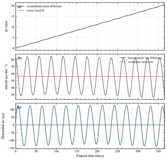
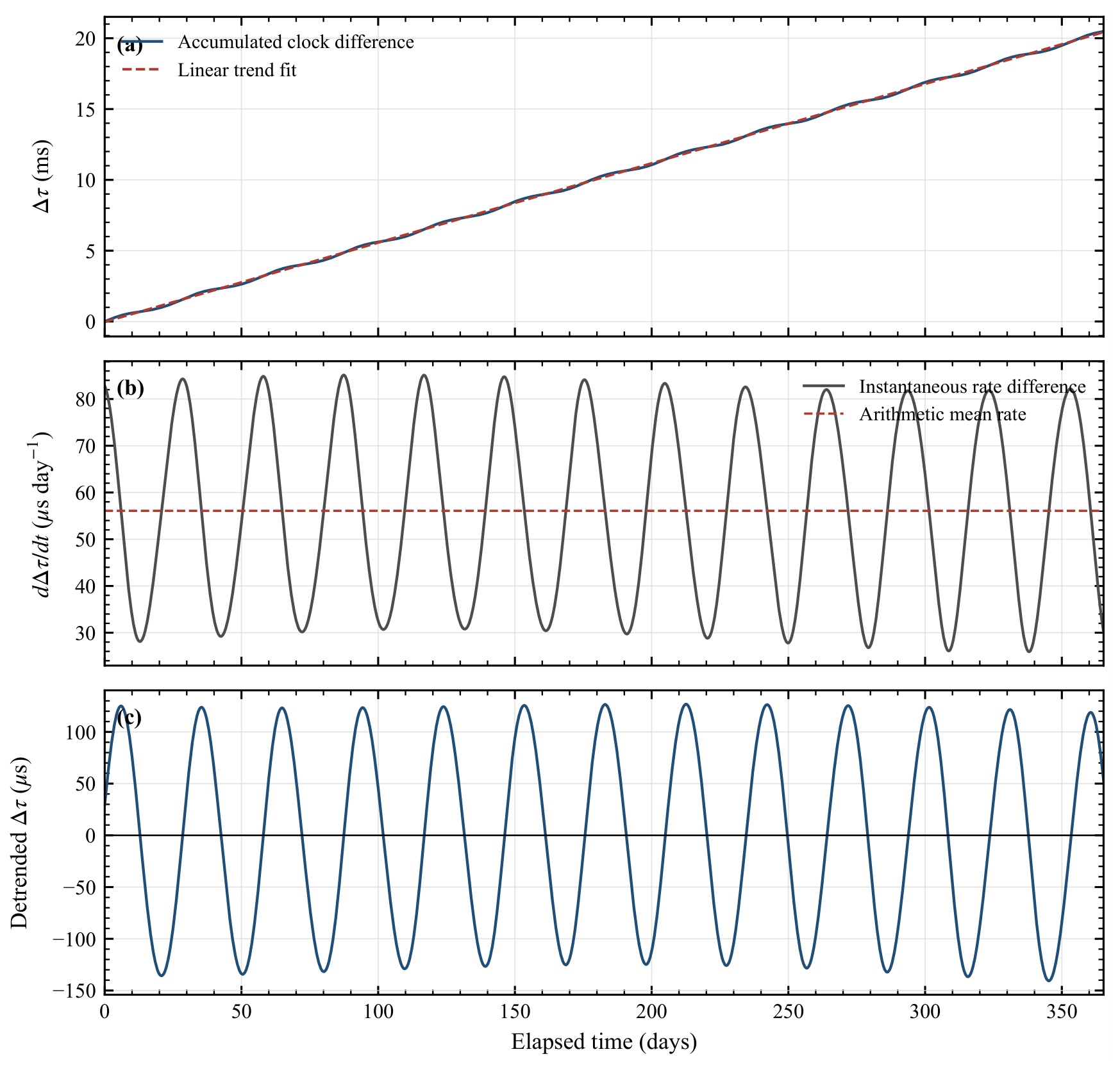
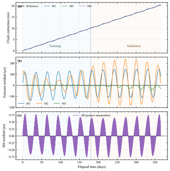
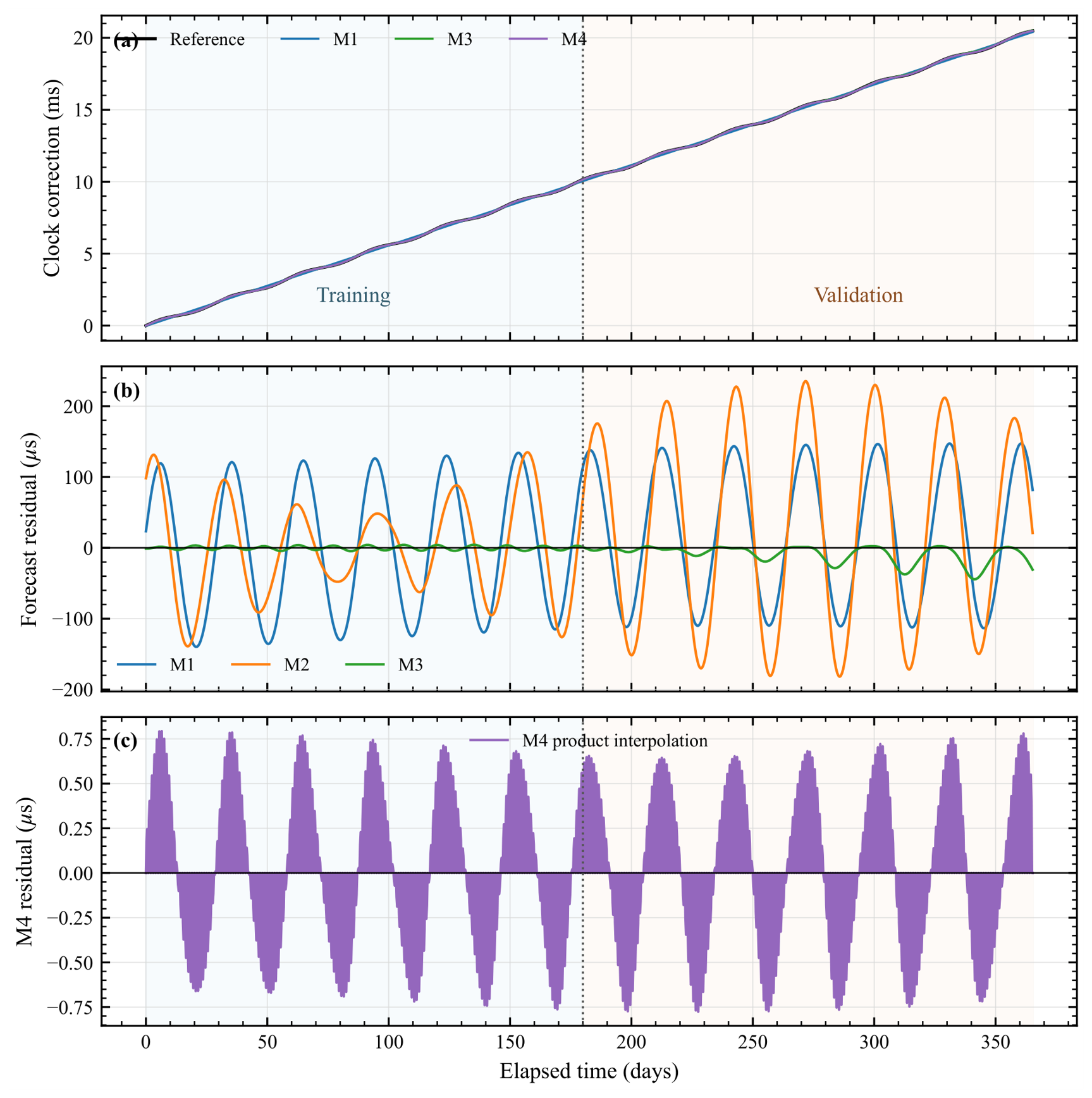
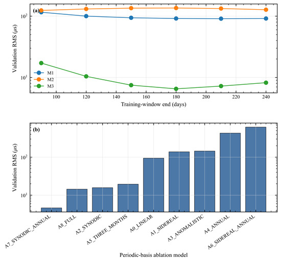
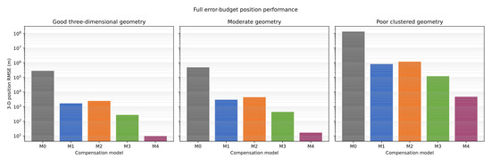
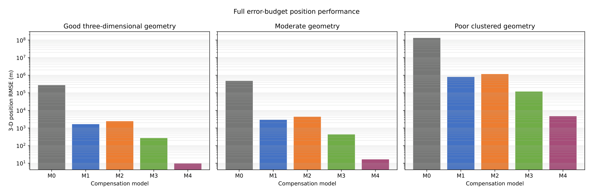
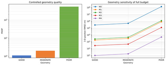
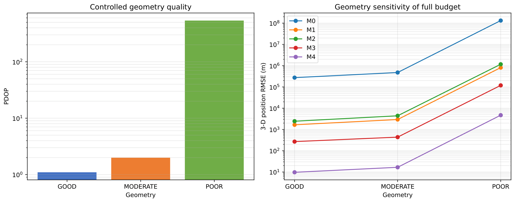

Disclaimer/Publisher’s Note: The statements, opinions and data contained in all publications are solely those of the individual author(s) and contributor(s) and not of MDPI and/or the editor(s). MDPI and/or the editor(s) disclaim responsibility for any injury to people or property resulting from any ideas, methods, instructions or products referred to in the content. |
© 2026 by the author. Licensee MDPI, Basel, Switzerland. This article is an open access article distributed under the terms and conditions of the Creative Commons Attribution (CC BY) license.