Real Estate Mass Appraisal Using Spatial Filtering with Moran’s Eigenvectors

Abstract

Mass appraisal of real estate is a central challenge for municipal tax administration, which must estimate assessed values fairly. Real estate market is strongly related to location, which is difficult to measure. Spatial autocorrelation in property prices violates ordinary least squares assumptions and potentially biases inference. This study investigates Moran’s Eigenvector Spatial Filtering (ESF) and its random-effects specification (RE-ESF) for land price modeling, comparing them with a hedonic ordinary least squares model and three classical spatial specifications (SAR, SEM, and SARAR). The analysis uses 2635 urban land records from Fortaleza, Ceará, Brazil, the country’s fourth most populous city, with a real estate stock exceeding 850,000 properties, and a row-standardized 30-nearest-neighbor weights matrix. All compared models share the same explanatory variables and are validated out of sample on the same random 80/20 partitions, compared in paired tests; residual autocorrelation is assessed against the Cliff–Ord null hypothesis, the appropriate reference for regression residuals. The filtered models remove the residual autocorrelation left by the unfiltered model and improve out-of-sample accuracy by a small but consistent margin: 0.022 in R² for ESF in 18 of 20 partitions, with the spatial error model as the closest classical competitor in R², though it is the worst of the four unfiltered specifications in mean absolute percentage error. The conclusions hold for neighborhood sizes from 10 to 40 and under a distance band. By removing the spatially systematic component of assessment error, spatial filtering improves the geographic dimension of assessment equity and thereby supports municipal fiscal management.

1. Introduction

Property valuation plays an important role in society and serves multiple purposes. At the municipal level, it supports property taxation, especially by determining assessed values for taxes such as the Property Tax and the Sales Tax, as well as other tributes based on property assessment. It also contributes to urban planning, public policies, and compensation in expropriation processes. In the private sector, it supports financing and real estate credit operations.

In this context, mass appraisal is prominent and can be understood as valuing multiple properties on a single reference date using statistical and standardized methods [1]. Essential for tax fairness, it allows for accurate estimation of assessed property values. However, outdated Property Value Maps in many municipalities can understate values and reduce property tax revenues [2,3,4]. Therefore, choosing appropriate mass appraisal methodologies is crucial.

According to McCord et al. [5], the hedonic pricing model, proposed by Rosen [6], was long the main technique used in real estate appraisal, modeling property prices as a function of their characteristics. However, hedonic regression models rely on assumptions, including data independence, which may limit their applicability in scenarios with strong spatial dependence, as in real estate markets. This occurs because nearby properties tend to have similar prices due to shared infrastructure and public services, access to the same amenities, and similar physical and socioeconomic characteristics [7]. This phenomenon is well described by the well-known “First Law of Geography,” which states that things closer together are more related than those farther apart [8].

Therefore, observed property prices exhibit an organized and structured spatial pattern. Regression models reveal spatial dependence through spatial autocorrelation in the residuals. In this sense, the residuals reflect unexplained variation attributable to the underlying spatial structure that the model has not properly accounted for, leading to biased and inconsistent parameter estimates [9,10].

In the context of mass appraisal for taxation, these effects may result in a regressive and inequitable tax system, in which clusters of positive residuals indicate undervaluation. Similarly, negative clusters signal overvaluation, leading to a disproportionate tax burden for certain taxpayers.

Given this issue, spatial econometrics offers a broad set of tools for addressing spatial dependence. Examples include the Spatial Autoregressive Model (SAR) [11], Spatial Error Model (SEM) [11], Spatial Autoregressive Combined Model (SARAR) [12,13,14], Generalized Additive Models (GAM) [15], Generalized Additive Models for Location, Scale, and Shape (GAMLSS) [16], and Geographically Weighted Regression (GWR) [17].

Another approach to mitigate these undesirable effects in mass appraisal is Moran’s Eigenvector Spatial Filtering (ESF) [18], which captures and models spatial dependence in the data, reduces autocorrelation in the residuals, and improves estimate accuracy. More recently, ESF has also been incorporated into machine learning models [5,19,20].

In this context, the study investigates the ESF technique, in its fixed-effects and random-effects forms, as an approach to spatial dependence on urban land prices. To this end, it compares their performance with a hedonic ordinary least squares model and with the classical spatial specifications SAR, SEM and SARAR, under out-of-sample validation on common partitions and a residual diagnostic appropriate to regression residuals. The empirical setting is Fortaleza, Ceará, Brazil, the country’s fourth most populous city, whose real estate stock of more than 850,000 properties makes mass appraisal a recurring administrative task and a demanding test case for the method.

2. Materials and Methods

2.1. Study Area and Dataset

This research adopted a quantitative, exploratory approach, using classical and spatial econometric techniques to model and predict real estate prices for urban land parcels of up to 10,000 m², considering land without buildings. Large land parcels, also known as “tracts of land,” were excluded from the sample. This decision is justified because such properties exhibit markedly different market characteristics, both in price formation and in potential uses. A tract of land is typically negotiated under specific conditions, often involving transactions related to land development, subdivision, or parceling, which make it incompatible with valuation mechanisms applicable to typical urban land parcels. Their inclusion could compromise sample homogeneity and introduce bias into the econometric models.

The study used 2635 data points from real estate transactions, sales tax assessments, and market listings, all georeferenced and collected from public and private sources related to the Municipality of Fortaleza, a state capital in Northeast Brazil and the fourth most populous city in the country, with a real estate stock exceeding 850,000 properties. The data span covers 2022 to 2024, ensuring that property values reflect recent market conditions while minimizing the impact of structural changes and long-term economic cycles.

Pooling transactions, tax assessments, and market listings in a single sample requires clarifying which value concept the fitted models estimate. These three sources are not directly comparable: market listings tend to reflect asking prices before negotiation, actual transactions reflect realized market value, and tax assessments reflect an administratively determined assessed value that is typically more conservative. As shown in Section 3.1, this hierarchy is consistent across all three years of the sample, with listing prices exhibiting the highest medians, followed by transaction prices, and tax-assessed values consistently the lowest. Rather than treating this heterogeneity as a source of bias to be eliminated, it is explicitly modeled through the dummy variables tr (transaction) and of (offer/listing), with tax assessment as the reference category; the corresponding coefficients, reported in Section 3, quantify the systematic difference in market-based sources over assessed values. Under this specification there is a single appraisal target rather than a hybrid of value concepts: in the mass appraisal conducted for taxation in Brazil, the transaction value is adopted as the assessed value, so the model estimates the assessed value, which in this institutional setting is the transaction value, and the source indicators absorb the systematic differences in level between listings, transactions and assessments. This treatment follows standard mass appraisal practice, where administrative and market-derived data are routinely combined, and their systematic level differences accounted for through source indicators. It does not, however, allow source-specific slopes: we did not test whether individual covariates (e.g., pvacp or lotcond) affect price differently across transaction types, and this remains a direction for future stratified analysis.

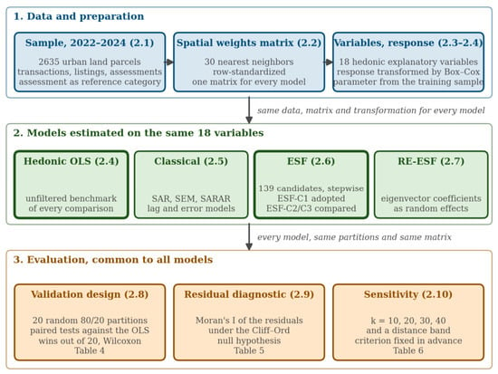
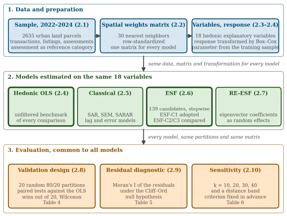
Figure 1 summarizes the analysis workflow and the subsections in which each step is described.

Figure 1. Workflow of the analysis. The three data sources are pooled into one sample; a single row-standardized 30-nearest-neighbor matrix is used by every model and diagnostic; the hedonic OLS is the benchmark, and the spatial models, classical and eigenvector-based, are estimated on the same 18 explanatory variables and evaluated on the same 20 partitions, with the residual diagnostic under the Cliff–Ord null hypothesis and a sensitivity analysis of the weights matrix. Numbers in parentheses are the subsections. Source: Developed by the authors.

2.2. Construction of the Spatial Weights Matrix

Based on the geolocation of the sample data, we constructed a spatial weights matrix W using a k-nearest neighbors approach, considering the 30 nearest neighbors for each observation. The matrix W was row-standardized, meaning that each element was divided by the sum of the weights in its row, yielding the incidence matrix C [21]. Therefore, each element of C, denoted as c_ij, is given by Equation (1):

$$c_{\mathit{ij}}={\displaystyle \frac{w_{\mathit{ij}}}{{\displaystyle {\sum }_{j=1}^n}{w}_{\mathit{ij}}}}$$

(1)

where w_ij is the element in row i, column j of the spatial weight matrix, and n is the total number of observations. By definition, the elements of the main diagonal are zero (w_ii = 0, ∀i), meaning that no observation is considered a neighbor of itself.

Next, this matrix was transformed according to Equation (2) [10]:

$${\mathrm{C}}^{*}=\left(\mathrm{I}-{\displaystyle \frac{{11}^{\mathrm{T}}}{n}}\right)\mathrm{C}\left(\mathrm{I}-{\displaystyle \frac{{11}^{\mathrm{T}}}{n}}\right)$$

(2)

where C* is the transformed spatial weights matrix; I is the identity matrix of dimension n × n; 1 is a column vector of dimension (n × 1) containing only ones; C is the incidence matrix; and the superscript “T” denotes the matrix transpose operator. Griffith and Peres-Neto [21] emphasize that by applying the same term to both the left and right sides of matrix C, a term referred to as the “centering operator”, the mean of the matrix weights is removed, thereby eliminating global effects and retaining only local neighborhood variations. According to these authors, this procedure ensures that the eigenvectors of matrix C* are orthogonal and linearly independent.

Subsequently, the spectral decomposition [22] of matrix C* was performed [10], as shown in Equation (3), to extract its corresponding eigenvectors and eigenvalues:

C^* = EΛE^T

(3)

where Λ = diag(λ₁, λ₂, ⋯, λ_m) is the diagonal matrix containing the m eigenvalues in descending order; and E = [E₁, E₂, …, E_m] is the matrix whose columns are the corresponding m eigenvectors. As previously mentioned, the centering performed by Equation (2) ensures that the eigenvectors are orthogonal, thus avoiding redundancy of spatial information, and, being linearly independent, each represents a unique spatial pattern. This gives rise to the name ESF, as the eigenvectors effectively act as “spatial filters,” revealing underlying latent spatial patterns in the data. Griffith and Chun [10] emphasize that these eigenvectors can be incorporated into the classical regression equation, as they do not alter the conditional mean of the dependent variable, since each eigenvector has a mean equal to zero (due to the centering of matrix C described above). However, a k-nearest-neighbor relation is directed, so the matrix defined in Equation (1) is not symmetric, and the transformation in Equation (2) preserves that asymmetry, whereas the decomposition in Equation (3) is defined for a symmetric operator. The eigenvectors were therefore extracted from the symmetric part of the transformed matrix, (C* + C*^T)/2, under which the orthonormality and the zero mean invoked above hold exactly.

2.3. Variables Used

Taking the unit price of land as the dependent variable, explanatory variables of a structural nature were selected a priori, that is, variables related to the physical attributes of the land parcels, as well as variables associated with their location, such as geographic position, distance to value-enhancing centers, distance to value-depreciating centers, distance to main roads, income of the household head in the surrounding area according to the most recent census [23], as well as variables related to the temporal dimension of the observations (year) and the source of the information (whether derived from listings, actual transactions, or sales tax assessments). Table 1 presents further details about these variables.

Table 1. Description of the dependent variable and explanatory variables.

Variable	Description	Type
punit	Unit price observed for each land plot, in R$/m2.	Dependent
lotcond	0—Outside a closed condo; 1—Inside a closed condo.	Location
numfr	Number of faces to the street.	Structural
esq	0—Land is not positioned on a corner; 1—It is on a corner.	Structural
f_inc	0—Land is not suitable for building development; 1—It is Suitable for development.	Location
pvsem	0—With paving; 1—With no paving.	Location
pvped	0—Without paving in rustic stone or cobblestone on any frontage of the property; 1—With.	Location
pvacp	0—Without any asphalt, concrete, or pre-cast paving in front of the property; 1—With one of them.	Location
renda	Kriged income of the household leader [21].	Location
dv	Verticalization density: Represents the concentration of vertical condominiums with elevators obtained by kernel interpolation with a quartic function of radius 200 m.	Location
dscom	Lot sales density for lots located on the same street section as the current lot.	Location
acasamed	IDW interpolation within a 500 m radius of the median built-up area of residential houses (decay power = −2).	Location
iamaxeq	Equivalent utilization index.	Location
pzpa1	Percentage of preservation area (ZPA1).	Location
distpv	Distance in m to the nearest value-influencing pole.	Location
distassp	Distance in m to the nearest informal settlement.	Location
distsh	Distance in m to the nearest shopping center.	Location
distbm	Distance in m to the Beira Mar Avenue promenade.	Location
distvp	Distance in m to the nearest main road.	Location
distvs	Distance in m to the nearest secondary road.	Location
test	Length of the main frontage in meters.	Structural
areater	Land size in m2.	Structural
a20xx	Set of dichotomous variables referring to the year of the price collection date (a2022, a2023, a2024)	Time
tr	0—is not a transaction; 1—It is a transaction.	Information class
of	0—It is not an offer; 1—It is an offer.	Information class

Source: Collected by the authors.

2.4. Multiple Linear Regression Model

The unfiltered baseline model is a multiple linear regression estimated by Ordinary Least Squares (OLS) on the variables described in Section 2.3. We removed variables that were not statistically significant at the 5% level and applied logarithmic transformations to some continuous covariates, as listed below. We verified the model assumptions: normality of residuals, homoscedasticity, and multicollinearity. The filtered models are compared against it both in the selected performance metrics and in the reduction in spatial autocorrelation in the residuals. We also estimated the same specification under the classical spatial econometric models of Section 2.5.

The hedonic specification uses 18 explanatory variables: lotcond, esq, pvacp, pzpa1, acasamed, iamaxeq, the year and source indicators (a2023, a2024, tr, of), and the natural logarithms of renda, dscom, distpv, distassp, distsh, distbm, distvp, and areater. The remaining variables of Table 1 (numfr, test, dv, distvs, f_inc, pvsem and pvped) are not part of this specification. The response is transformed by Box–Cox, with the parameter estimated by maximum likelihood on the response alone, on the training data of each partition (Section 2.8), and the hedonic OLS on the Box–Cox response is the benchmark of every comparison in Section 3.6 and Section 3.7.

2.5. Classical Spatial Econometric Models

We estimated three classical spatial econometric specifications as benchmarks so that the contribution of the eigenvector approach, presented in Section 2.6 and Section 2.7, is measured against standard alternatives rather than against the non-spatial model alone. The spatial autoregressive model (SAR) introduces a spatially lagged dependent variable, y = ρWy + Xβ + ε, so that the price of a parcel depends on the prices of its neighbors. The spatial error model (SEM) leaves the conditional mean unchanged and places the dependence in the disturbance, y = Xβ + u with u = λWu + ε. The SARAR specification combines both channels, allowing simultaneously for a lag in the dependent variable and autocorrelation in the error. The symbol λ is the conventional notation for the error parameter and is unrelated to the Box–Cox parameter and the eigenvalues in Section 2.2, which share it.

We estimated the three models using the same 18 hedonic explanatory variables, the same Box–Cox transformation of the response, and the same row-standardized 30-nearest-neighbor weights matrix used by the eigenvector models and validated them on the same partitions described in Section 2.8. We estimated SAR and SEM by maximum likelihood, and SARAR by the generalized method of moments, as implemented in the spreg module (version 1.8.2) of PySAL (version 25.1).

2.6. Moran’s Eigenvector Spatial Filtering

Following classical OLS and spatial econometric models, we applied the ESF approach. For this purpose, we developed an original script in Python (version 3.12.8) and used the spmoran library (version 0.3.3), implemented in R (version 4.4.2) by Murakami [24], to support advanced ESF modeling.

The first approach, implemented in Python, began with the spectral decomposition of matrix C*, as presented in Equation (3). For the selection of the most relevant eigenvectors, the two-step criterion of Griffith and Chun [10], later formalized as the standard forward stepwise by Chun, Griffith, Lee and Sinha [25], was adopted:

(i)

Pre-selection based on eigenvalues: after extracting and sorting all eigenvalues and their corresponding eigenvectors in descending order, only those satisfying the condition λ_i/λ₁ ≥ 0.25 were retained;

(ii)

Further selection of eigenvectors through a “forward stepwise” procedure: from the pre-selected subset, eigenvectors were sequentially introduced into the model, following the descending order of their eigenvalues, provided they were statistically significant at the 5% level and contributed to an increase in the adjusted coefficient of determination (R²_adj).

The criterion adopted in this study, denoted ESF-C1 in what follows, is the standard forward stepwise of Chun, Griffith, Lee and Sinha [25]: steps (i) and (ii) above, and nothing further. We estimated two alternatives for comparison, with the set of candidate criteria fixed before running either one, so the comparison is a test rather than a selection. ESF-C2 admits, at each step, the eigenvector that most reduces the absolute residual Moran coefficient and stops when that coefficient ceases to be significant. ESF-C3 minimizes the corrected Akaike information criterion, with no significance constraint. On the full sample, the three retain 39, 19 and 63 eigenvectors respectively.

The three criteria are compared on predictive performance, on the residual diagnostic of Section 2.9, and on parsimony, and the comparison is reported in Section 3.6 and Section 3.7. Reporting all three, rather than the adopted one alone, is what allows the basis of the choice to be examined.

Although pre-selection was based on descending eigenvalue order, the subsequent stepwise forward selection procedure did not guarantee that eigenvectors would be introduced in the same order. This is due to the conditional nature of the implemented procedure, which, at each iteration, evaluated all remaining candidates and incorporated only the one that maximized the increase in R²_adj, while satisfying the significance constraint of step (ii). As a result, eigenvectors associated with smaller eigenvalues could be included before others with larger magnitudes, provided their marginal contribution to model fit was more relevant.

The mathematical formulation of the ESF model, with n observations, m extracted eigenvectors, and p explanatory variables, is given in Equation (4) in matrix form:

y = X·β + Eγ + ε

(4)

where β is the vector of fixed coefficients associated with the explanatory variables; E is the n × m matrix of Moran’s spatial eigenvectors (MEs); γ represents the fixed coefficients associated with the eigenvectors; and ε is the vector of random errors, assumed to be independent and identically distributed (i.i.d.), such that ε ~ N(0, σ²I). It should be noted that a Box–Cox transformation was applied to the original dependent variable (unit land price in R$/m²—the Brazilian Real, Brazil’s currency, per square meter) before parameter estimation.

2.7. Random Effects Eigenvector Spatial Filtering

In addition to the ESF model, we estimated the Random Effects Eigenvector Spatial Filtering (RE-ESF) model using the spmoran library’s “resf” function. The RE-ESF extends the ESF approach by modeling the eigenvector coefficients as random effects rather than fixed effects. Furthermore, it incorporates robust nonparametric transformations of the dependent variable, including Box–Cox transformations and nonlinear approximations, directly within the “resf” function of the spmoran library.

Specifically, the “nongauss_y” function from the spmoran library was used with one transformation term (“tr_num” = 1), which is suitable for continuous and non-negative variables (essentially corresponding to the Box–Cox transformation). The mathematical formulation of the RE-ESF model is given in Equation (5):

y = X·β + Eu + ε

(5)

where y is the n × 1 vector of the dependent variable; X is the n × p matrix of explanatory variables; β is the p × 1 vector of fixed coefficients associated with the explanatory variables; E is the n × m matrix of Moran’s spatial eigenvectors (MEs); u is the m × 1 vector of spatial effects associated with the eigenvectors in E. In the RE-ESF model, these effects are not estimated individually but are assumed to follow a multivariate normal distribution: u ~ N(0, ${\sigma }_u^2{\mathrm{I}}_m$). This implies that each component of u has zero mean, variance ${\sigma }_u^2$, and that they are mutually uncorrelated. The parameter ${\sigma }_u^2$ summarizes the intensity of spatial dependence captured by the eigenvectors; ε is the vector of random errors, assumed to be independent and identically distributed (i. i. d.), such that ε ~ N(0, σ²I_n).

After estimating the ESF and RE-ESF models, residual spatial autocorrelation was assessed with Moran’s I on the same spatial weight’s matrix used for the unfiltered model, against the Cliff–Ord reference of Section 2.9, to verify whether the filter removed the spatial dependence not captured by the explanatory variables.

Additionally, to visually interpret the spatial pattern captured by the selected Moran eigenvectors, a map of the estimated spatial component (Eu), corresponding to the second term in Equation (5), was generated. This mapping made it possible to identify areas of the city where spatial effects not directly explained by the original explanatory variables are present, providing relevant insights for analyses of heterogeneity and segmentation in the real estate market.

2.8. Validation Design and Statistical Inference

The performance measures reported for the models described above are obtained out of sample. The reason lies in the nature of the filter: the eigenvectors add many covariates to the regression, so in-sample fit cannot distinguish genuine predictive improvement from overfitting, and an in-sample comparison between a filtered and an unfiltered model is uninformative about predictive performance.

Partitioning. We split the 2635 parcels into 80% for estimation and 20% for testing, stratified by data source and year so that the three sources and three years appear in both parts in the same proportions. Every quantity that depends on the data is computed on the training subsample only: the spatial weights matrix, the eigenvector extraction, the stepwise selection, the Box–Cox parameter, and the regression coefficients. Eigenvector values at the test locations are obtained from the training points: the value of each eigenvector at a test parcel is the mean of its values over the 30 nearest training parcels, which is the numerator of the Nyström extension [26]—the standard method for estimating a spectral eigenvector’s value at an out-of-sample point—without the division by the eigenvalue that the full method applies. This attenuates eigenvectors of small eigenvalues more than those of large eigenvalues, by a factor of up to 3.46 among the 39 selected; the net effect of that attenuation on predictive accuracy is of unknown sign and is left unquantified.

Repetition. A single split is a weak basis for ranking models because variation between splits is large relative to differences between models. The exercise is therefore repeated over 20 partitions, generated with seeds 1000 to 1019, and the same 20 partitions are used for every model reported in this paper. Results are presented as bands, the mean ± standard deviation over the 20 repetitions, rather than as single numbers.

Metrics. Predictions are transformed back to the original scale, and all out-of-sample measures (R² computed as 1 − SSE/SST and MAPE) are expressed in R$/m². This makes the out-of-sample figures comparable across models estimated on different response transformations, a comparability that the in-sample adjusted R² does not provide. The back-transformation is applied without a correction for retransformation bias, so the out-of-sample measures are conservative; since every model is treated identically, the paired comparisons are unaffected.

Paired inference. Because every model is evaluated on the same 20 partitions, we compare models pairwise: for each partition, we compute the difference between two models and run inference on the 20 differences rather than on the two sets of 20 levels. The reason is quantitative. The standard deviation of out-of-sample R² across partitions is approximately 0.055, whereas the standard deviation of the paired differences is between 0.015 and 0.018. A difference of 0.02 is therefore not detectable when comparing the two distributions marginally but is detectable when the comparison is paired. Reading a paired difference against the between-partition standard deviation, or the reverse, would invalidate the conclusion.

The hypothesis of no difference is assessed with the Wilcoxon signed-rank test, which tests whether the median of the paired differences is zero without assuming that those differences are normally distributed; with 20 pairs, normality would be an assumption that the design does not support. The paired t-test is reported alongside it; the two are always reported together, and any disagreement between them is stated. The number of partitions in which one model outperforms the other is also reported, since it is the most direct summary of the comparison and requires no distributional assumption.

Limitation of the design. The partitions are random, not spatial. Test parcels are therefore interspersed among training parcels, a configuration that favors any model exploiting immediate neighborhood information. The out-of-sample gains reported in Section 3 should accordingly be read as an upper bound on spatial generalization rather than as a lower bound. A block design, which would measure generalization to unsampled areas, is discussed in Section 4 as an extension of this work.

2.9. Testing for Residual Spatial Autocorrelation

This paper uses Moran’s I under two different null hypotheses. In the exploratory analysis of Section 3.1, it tests whether the observed unit price clusters in space, against the null that values are assigned to locations at random, for which E[I] = −1/(n − 1) ≈ 0. In Section 3.2, Section 3.3, Section 3.4, Section 3.5, Section 3.6, Section 3.7 and Section 3.8 it is applied to regression residuals instead, which are correlated by construction (e = My) even without spatial structure; the appropriate reference there is the Cliff–Ord null hypothesis, under which E[I] = (n/S0)·tr(MW)/(n − k), a negative value whose magnitude grows with the number of parameters k.

Because this expectation is model-specific, residual statistics in this paper are always read against it, not against zero, and both are reported alongside each statistic in Section 3.7. A residual I slightly below zero is not, by itself, evidence of over-filtering, and residual statistics are not directly comparable across models with different k.

2.10. Robustness of the Spatial Weights Matrix

The choice of 30 nearest neighbors is not the outcome of an optimization, and a sensitivity analysis was designed to establish whether the conclusions depend on it. Five matrices are compared: k-nearest-neighbor (kNN) graphs with k = 10, 20, 30, and 40, and a distance band of 1795 m, which is the smallest radius that leaves no parcel without neighbors. All five are row-standardized.

The criterion for robustness was fixed before the analysis was carried out: the conclusions are treated as robust if the filtered model outperforms the hedonic OLS in the paired comparison under all five matrices, and if the residual Moran’s I of the filtered model is not significant under the reference of Section 2.9 under all or nearly all of them. Declaring the criterion in advance matters, because the alternative, inspecting the results and then selecting which matrix to report, would turn a test into a selection. In particular, a matrix that happened to outperform k = 30 would not authorize revising that choice after the fact; it would only qualify the interpretation of the chosen value, as Section 3.8 does.

3. Results and Discussion

3.1. Exploratory Analysis

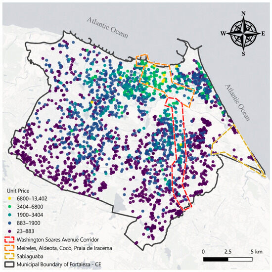
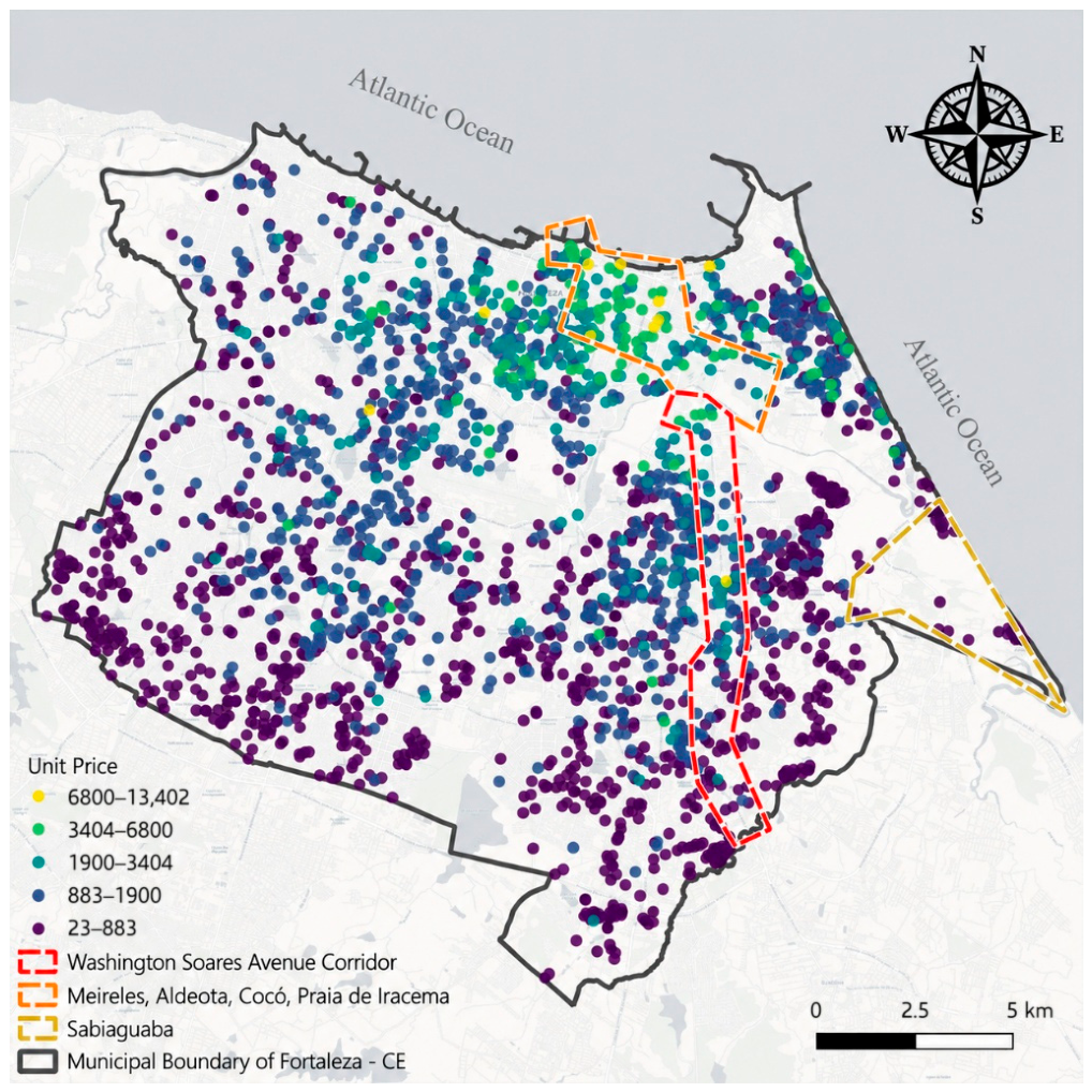
Figure 2 presents a thematic map of the spatial distribution of the land parcels included in the dataset, along with their respective unit price ranges (R$/m²).

Figure 2. Study area with spatial distribution of urban land (values expressed in Brazilian reais per square meter (R$/m²); coordinates in SIRGAS 2000, zone 24S). Source: Developed by the authors.

From Figure 2, it can be observed that the highest-valued land parcels are in the northern and central parts of the city, corresponding to neighborhoods such as Meireles, Aldeota, Cocó, and Praia de Iracema. Another value-enhancing axis runs along Washington Soares Avenue, which passes through important neighborhoods such as Guararapes and Edson Queiroz. The least-valued areas are distributed across the western and southern parts of the city, as well as in the far eastern region, particularly in the Sabiaguaba neighborhood.

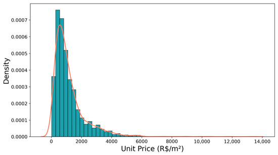
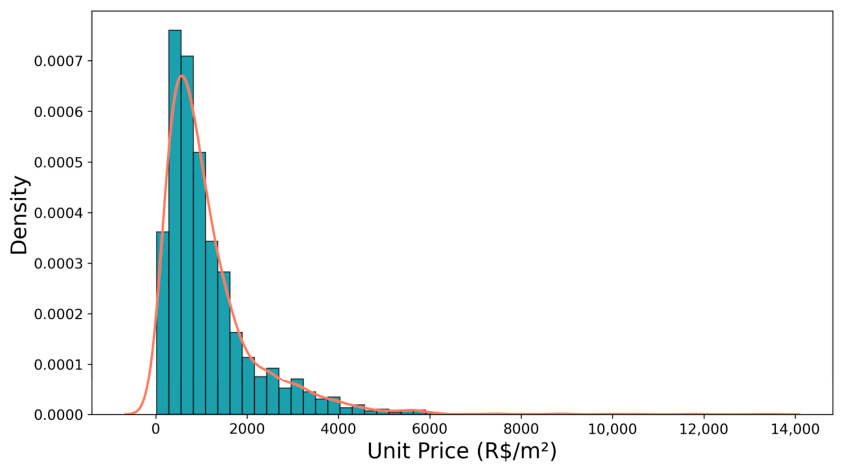
Figure 3 presents the distribution of unit land prices (in R$/m²) observed in the sample. A right-skewed distribution is evident, with a strong concentration of values in lower price ranges and a long tail extending up to R$ 13,400/m². This pattern is typical of real estate markets, where most properties are in lower-value areas. At the same time, a relatively small number reach much higher prices, generally associated with privileged locations with higher demand and land scarcity, especially for real estate development.

Figure 3. Histogram of unit land prices, with the kernel density estimate (red line). Source: Developed by the authors.

The presence of this asymmetry suggests the need for a variable transformation, such as the natural logarithm or a Box–Cox transformation, to meet the normality assumption of the residuals in regression models.

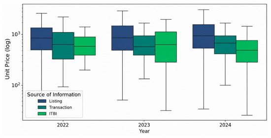
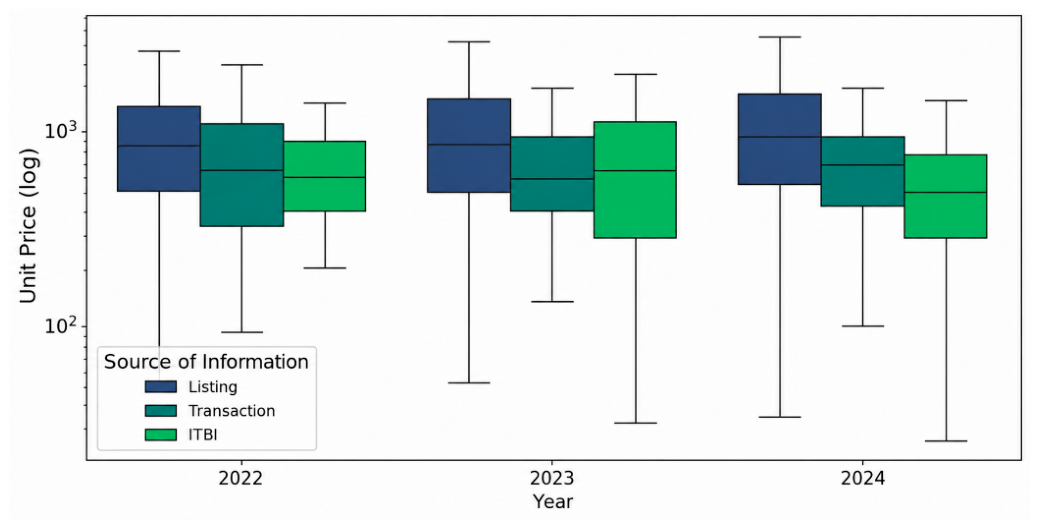
Figure 4 shows the variation in unit land prices (on a logarithmic scale) according to year and data source (listing, transaction, and sales tax files) for the period from 2022 to 2024. The logarithmic scale on the y-axis was chosen to emphasize the asymmetry and facilitate visual comparison between groups.

Figure 4. Boxplot of the variation in unit land prices (on a logarithmic scale) according to year and data source (listing, transaction, and sales tax files) for the period from 2022 to 2024. In the legend, ITBI stands for Imposto sobre a Transmissão de Bens Imóveis, the municipal sales tax: its files provide the tax-assessed values, the reference category of the source indicators; Listing and Transaction are the market listings and the realized transactions. Source: Developed by the authors.

Across all three years, values derived from listings tend to have higher medians, followed by transaction data, with the lowest values in sales tax declarations. This hierarchy suggests a pattern of “overpricing” in listings relative to transaction prices and, in turn, a possible underreporting of values for tax purposes. Dispersion is high across all categories, reflecting the heterogeneity of the real estate market.

Supplementary Table S4 presents the descriptive statistics of the quantitative variables tested in the model, excluding the dummy variables.

Supplementary Figure S1 shows the spatial connectivity graph of the weight’s matrix, with parcels as vertices and neighbor relations as edges.

To assess the existence of spatial dependence in unit land prices, the global Moran’s I index was initially estimated. The obtained value was 0.48, statistically significant at the 1% level (p = 0.0010), indicating positive spatial autocorrelation. This result shows that land parcels with similar unit prices tend to be located near one another, thereby characterizing the formation of spatial clusters. As noted earlier, spatial dependence may also be present in a regression model’s residuals, violating the assumption of error independence and compromising the validity of classical inferences.

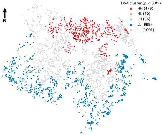
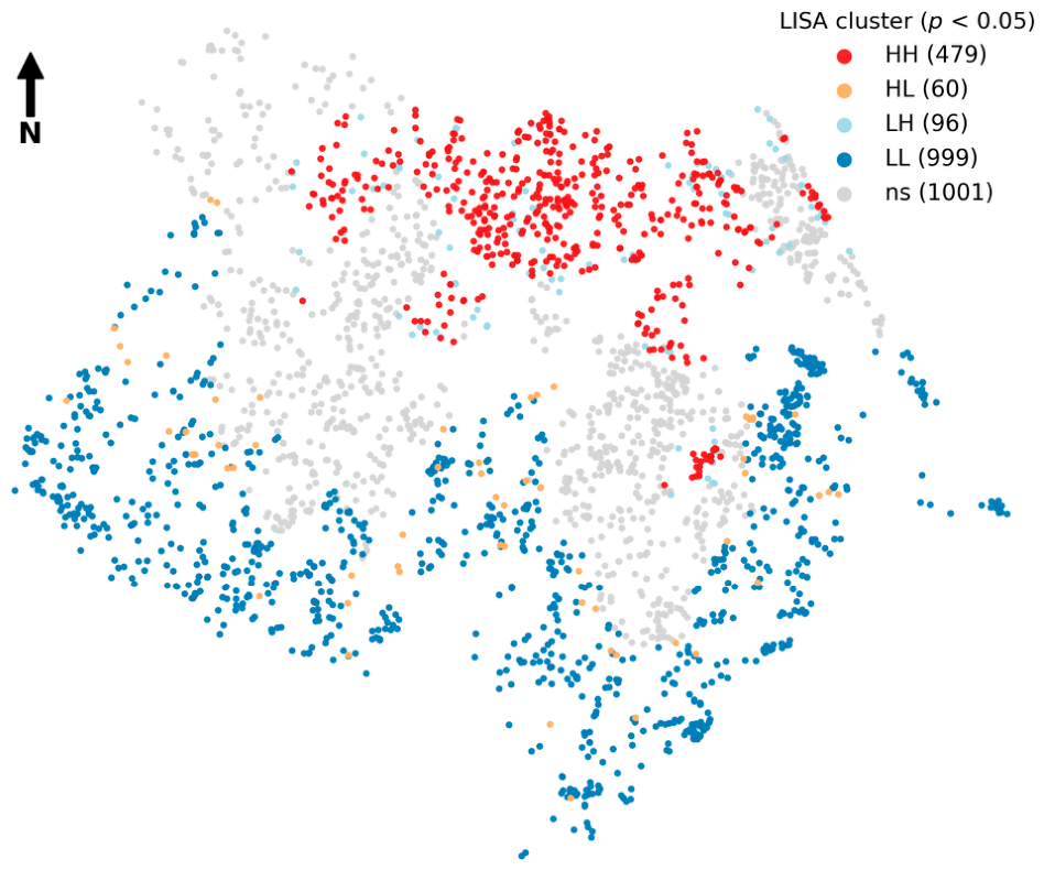
Subsequently, the Local Indicators of Spatial Association (LISA) statistic [11], shown in Figure 5, was applied to further examine the spatial distribution of these clusters and identify specific areas of high and low concentration. This statistic identifies spatial clusters of similar or dissimilar values, revealing local patterns not captured by the global Moran’s I index.

Figure 5. LISA cluster map of unit land prices (R$/m²) (p < 0.05). Source: Developed by the authors.

Figure 5 shows the spatial distribution of clusters on the map. Observations shown in red and labeled HH (high–high) represent land parcels with high values surrounded by neighbors with high values, corresponding to the city’s most valued areas. Dark blue points, labeled LL (low–low), represent land parcels with low unit values surrounded by neighbors with similarly low values, corresponding to more peripheral, lower-valued regions. Orange observations, labeled HL (high–low), represent land parcels with high values surrounded by low-value neighbors. These are less frequent and may indicate measurement errors, value transition zones, and gentrification processes, among other factors. Similarly, light blue observations, labeled LH (low–high), represent land parcels with low values surrounded by high-value neighbors. The remaining points, shown in gray (the majority), correspond to observations for which no statistically significant local spatial autocorrelation was detected at the 5% significance level.

3.2. OLS Results

The unfiltered baseline of Section 2.4 is the hedonic OLS estimated on the 18 original explanatory variables, with the response transformed by Box–Cox (λ = 0.0339). Table 2 reports the estimated coefficients. Within the sample, the model achieves an adjusted R² of 0.667, a root mean squared error of 735.9 R$/m², and a MAPE of 40.0%; all 18 covariates are significant at the 5% level, with the signs expected in the real estate market. Section 3.6 reports its out-of-sample performance, which underpins every comparison in this paper.

Table 2. Estimated coefficients of the hedonic OLS model.

Attribute	OLS
Intercept	7.5047 *** (0.4657)
lotcond	0.9037 *** (0.0893)
esq	0.1251 *** (0.0277)
pvacp	0.1796 *** (0.0293)
ln_renda	0.4737 *** (0.0378)
ln_dscom	0.2720 *** (0.0243)
acasamed	0.3607 ** (0.1498)
iamaxeq	0.0724 *** (0.0267)
pzpa1	−0.4380 *** (0.1573)
ln_distpv	−0.0969 *** (0.0140)
ln_distassp	0.0246 *** (0.0073)
ln_distsh	−0.0819 *** (0.0183)
ln_distbm	−0.2970 *** (0.0251)
ln_distvp	−0.1161 *** (0.0094)
ln_areater	−0.0329 *** (0.0124)
a2023	0.0910 *** (0.0288)
a2024	0.0872 *** (0.0283)
tr	0.2276 *** (0.0526)
of	0.3972 *** (0.0495)
Model parameters
Box–Cox λ	0.0339
Model statistics
Observations	2635
R2	0.669
R2adj	0.667
F-statistic	293.939 ***
Robust Wald statistic	285.654 ***
Log-likelihood	−2363.82
AIC	4765.65
BIC	4877.30

Notes: The dependent variable is transformed by Box–Cox and the model is estimated by ordinary least squares on the 18 hedonic explanatory variables. HC3 heteroskedasticity-consistent standard errors are reported in parentheses. *** p < 0.01, ** p < 0.05. The F-statistic is the conventional least-squares statistic; the heteroskedasticity-robust Wald statistic is reported alongside it. The log-likelihood, AIC, and BIC refer to the Box–Cox scale of the response, without the Jacobian of the transformation; they are comparable with those of Table 3, which refers to the same scale and estimator, and not with those of Supplementary Table S3. This model is the benchmark of every comparison in Section 3.6 and Section 3.7. Source: Developed by authors.

Table 2. Estimated coefficients of the hedonic OLS model.

Attribute	OLS
Intercept	7.5047 *** (0.4657)
lotcond	0.9037 *** (0.0893)
esq	0.1251 *** (0.0277)
pvacp	0.1796 *** (0.0293)
ln_renda	0.4737 *** (0.0378)
ln_dscom	0.2720 *** (0.0243)
acasamed	0.3607 ** (0.1498)
iamaxeq	0.0724 *** (0.0267)
pzpa1	−0.4380 *** (0.1573)
ln_distpv	−0.0969 *** (0.0140)
ln_distassp	0.0246 *** (0.0073)
ln_distsh	−0.0819 *** (0.0183)
ln_distbm	−0.2970 *** (0.0251)
ln_distvp	−0.1161 *** (0.0094)
ln_areater	−0.0329 *** (0.0124)
a2023	0.0910 *** (0.0288)
a2024	0.0872 *** (0.0283)
tr	0.2276 *** (0.0526)
of	0.3972 *** (0.0495)
Model parameters
Box–Cox λ	0.0339
Model statistics
Observations	2635
R2	0.669
R2adj	0.667
F-statistic	293.939 ***
Robust Wald statistic	285.654 ***
Log-likelihood	−2363.82
AIC	4765.65
BIC	4877.30

Notes: The dependent variable is transformed by Box–Cox and the model is estimated by ordinary least squares on the 18 hedonic explanatory variables. HC3 heteroskedasticity-consistent standard errors are reported in parentheses. *** p < 0.01, ** p < 0.05. The F-statistic is the conventional least-squares statistic; the heteroskedasticity-robust Wald statistic is reported alongside it. The log-likelihood, AIC, and BIC refer to the Box–Cox scale of the response, without the Jacobian of the transformation; they are comparable with those of Table 3, which refers to the same scale and estimator, and not with those of Supplementary Table S3. This model is the benchmark of every comparison in Section 3.6 and Section 3.7. Source: Developed by authors.

Table 3. Estimated coefficients of the ESF model.

Attribute	ESF
Intercept	8.8041 *** (0.5032)
lotcond	0.6696 *** (0.0839)
esq	0.1120 *** (0.0254)
pvacp	0.1493 *** (0.0287)
ln_renda	0.3566 *** (0.0413)
ln_dscom	0.2278 *** (0.0244)
acasamed	0.5208 *** (0.1526)
iamaxeq	0.1346 *** (0.0307)
pzpa1	−0.3880 *** (0.1259)
ln_distpv	−0.0534 *** (0.0118)
ln_distassp	0.0366 *** (0.0070)
ln_distsh	−0.1293 *** (0.0206)
ln_distbm	−0.3568 *** (0.0298)
ln_distvp	−0.1135 *** (0.0085)
ln_areater	−0.0371 *** (0.0112)
a2023	0.0892 *** (0.0284)
a2024	0.1020 *** (0.0277)
tr	0.2036 *** (0.0560)
of	0.4154 *** (0.0501)
EV_6	−3.1058 *** (0.7744)
EV_9	2.8515 *** (0.6045)
Model parameters
Box–Cox λ	0.0339
Candidate eigenvectors	139
Selected eigenvectors (ESF-C1)	39
Model statistics
Observations	2635
R2	0.714
R2adj	0.708
F-statistic (57 restrictions)	113.015 ***
Log-likelihood	−2170.67
AIC	4457.34
BIC	4798.19

Notes: The dependent variable is transformed by Box–Cox and the model is estimated by ordinary least squares on the 18 hedonic explanatory variables and the 39 eigenvectors selected under ESF-C1. Conventional least-squares standard errors are reported in parentheses; they are not the heteroskedasticity-consistent estimates of Table 2, and individual significance should be read with that qualification. *** p < 0.01. Of the 39 eigenvectors included in the model, the table reports the first two selected, EV_6 and EV_9. The F-statistic jointly tests the 57 slope restrictions in this specification and does not test the contribution of the eigenvectors. The log-likelihood, AIC and BIC refer to the Box–Cox scale, without the Jacobian of the transformation, and are comparable with those of Table 2, which refers to the same scale and estimator, but not with those of Supplementary Table S3, which refers to a different scale of the response and to a restricted-likelihood estimator. The comparison between models rests on the out-of-sample measures of Table 4. Source: Developed by authors.

Table 3. Estimated coefficients of the ESF model.

Attribute	ESF
Intercept	8.8041 *** (0.5032)
lotcond	0.6696 *** (0.0839)
esq	0.1120 *** (0.0254)
pvacp	0.1493 *** (0.0287)
ln_renda	0.3566 *** (0.0413)
ln_dscom	0.2278 *** (0.0244)
acasamed	0.5208 *** (0.1526)
iamaxeq	0.1346 *** (0.0307)
pzpa1	−0.3880 *** (0.1259)
ln_distpv	−0.0534 *** (0.0118)
ln_distassp	0.0366 *** (0.0070)
ln_distsh	−0.1293 *** (0.0206)
ln_distbm	−0.3568 *** (0.0298)
ln_distvp	−0.1135 *** (0.0085)
ln_areater	−0.0371 *** (0.0112)
a2023	0.0892 *** (0.0284)
a2024	0.1020 *** (0.0277)
tr	0.2036 *** (0.0560)
of	0.4154 *** (0.0501)
EV_6	−3.1058 *** (0.7744)
EV_9	2.8515 *** (0.6045)
Model parameters
Box–Cox λ	0.0339
Candidate eigenvectors	139
Selected eigenvectors (ESF-C1)	39
Model statistics
Observations	2635
R2	0.714
R2adj	0.708
F-statistic (57 restrictions)	113.015 ***
Log-likelihood	−2170.67
AIC	4457.34
BIC	4798.19

Notes: The dependent variable is transformed by Box–Cox and the model is estimated by ordinary least squares on the 18 hedonic explanatory variables and the 39 eigenvectors selected under ESF-C1. Conventional least-squares standard errors are reported in parentheses; they are not the heteroskedasticity-consistent estimates of Table 2, and individual significance should be read with that qualification. *** p < 0.01. Of the 39 eigenvectors included in the model, the table reports the first two selected, EV_6 and EV_9. The F-statistic jointly tests the 57 slope restrictions in this specification and does not test the contribution of the eigenvectors. The log-likelihood, AIC and BIC refer to the Box–Cox scale, without the Jacobian of the transformation, and are comparable with those of Table 2, which refers to the same scale and estimator, but not with those of Supplementary Table S3, which refers to a different scale of the response and to a restricted-likelihood estimator. The comparison between models rests on the out-of-sample measures of Table 4. Source: Developed by authors.

Table 4. Model comparison on the hedonic specification: out-of-sample performance over the same 20 partitions.

Model	Spatial Parameters	R2oos (Out-of-Sample; Mean ± SD)	MAPEoos (%; Mean ± SD)	Δ vs. OLS-BC (wins/20)
OLS, hedonic (log response)	—	0.5315 ± 0.0550	40.61 ± 2.75	−0.0006 (9/20)
OLS, hedonic (Box–Cox response)	—	0.5322 ± 0.0532	40.78 ± 2.77	benchmark
SAR (spatial lag, ML)	1 (ρ)	0.5177 ± 0.0446	41.06 ± 3.05	−0.0144 (5/20)
SEM (spatial error, ML)	1 (λ)	0.5386 ± 0.0547	42.03 ± 2.84	+0.0065 (15/20)
SARAR (lag and error, GMM)	2 (ρ, λ)	0.5248 ± 0.0468	41.26 ± 2.95	−0.0073 (7/20)
ESF-C1	39 eigenvectors	0.5542 ± 0.0569	38.62 ± 2.77	+0.0220 (18/20)
ESF-C1 (log response)	38 eigenvectors	0.5493 ± 0.0563	38.43 ± 2.77	+0.0171 (17/20)
ESF-C2	19 eigenvectors	0.5494 ± 0.0579	39.27 ± 2.66	+0.0172 (18/20)
ESF-C3	63 eigenvectors	0.5542 ± 0.0548	38.37 ± 2.74	+0.0220 (16/20)
RE-ESF	150 eigenvectors, ≈114.9 effective df	0.5584 ± 0.0581	38.42 ± 2.71	+0.0262 (19/20)

Notes: All models are estimated on the same 18 hedonic explanatory variables and validated on the same 20 partitions (Section 2.8). Out-of-sample measures are computed on the original scale (R$/m²) and are therefore comparable across models. Δ R²oos is the mean paired difference against the hedonic OLS estimated on the Box–Cox response, computed partition by partition; the figure in parentheses counts the partitions, out of 20, in which the model exceeds that benchmark. Rows are ordered by model families, not by performance. ESF-C1, ESF-C2 and ESF-C3 are defined in Section 2.6. The row with the logarithmic response is estimated and validated on that scale, and its paired difference is computed, like every other, against the Box–Cox benchmark on the original scale of prices; Section 3.6 reports its comparison with the OLS on the same scale. The partitions are random, not spatial, so the out-of-sample gains are an upper bound on spatial generalization (Section 2.8).

Table 4. Model comparison on the hedonic specification: out-of-sample performance over the same 20 partitions.

Model	Spatial Parameters	R2oos (Out-of-Sample; Mean ± SD)	MAPEoos (%; Mean ± SD)	Δ vs. OLS-BC (wins/20)
OLS, hedonic (log response)	—	0.5315 ± 0.0550	40.61 ± 2.75	−0.0006 (9/20)
OLS, hedonic (Box–Cox response)	—	0.5322 ± 0.0532	40.78 ± 2.77	benchmark
SAR (spatial lag, ML)	1 (ρ)	0.5177 ± 0.0446	41.06 ± 3.05	−0.0144 (5/20)
SEM (spatial error, ML)	1 (λ)	0.5386 ± 0.0547	42.03 ± 2.84	+0.0065 (15/20)
SARAR (lag and error, GMM)	2 (ρ, λ)	0.5248 ± 0.0468	41.26 ± 2.95	−0.0073 (7/20)
ESF-C1	39 eigenvectors	0.5542 ± 0.0569	38.62 ± 2.77	+0.0220 (18/20)
ESF-C1 (log response)	38 eigenvectors	0.5493 ± 0.0563	38.43 ± 2.77	+0.0171 (17/20)
ESF-C2	19 eigenvectors	0.5494 ± 0.0579	39.27 ± 2.66	+0.0172 (18/20)
ESF-C3	63 eigenvectors	0.5542 ± 0.0548	38.37 ± 2.74	+0.0220 (16/20)
RE-ESF	150 eigenvectors, ≈114.9 effective df	0.5584 ± 0.0581	38.42 ± 2.71	+0.0262 (19/20)

Notes: All models are estimated on the same 18 hedonic explanatory variables and validated on the same 20 partitions (Section 2.8). Out-of-sample measures are computed on the original scale (R$/m²) and are therefore comparable across models. Δ R²oos is the mean paired difference against the hedonic OLS estimated on the Box–Cox response, computed partition by partition; the figure in parentheses counts the partitions, out of 20, in which the model exceeds that benchmark. Rows are ordered by model families, not by performance. ESF-C1, ESF-C2 and ESF-C3 are defined in Section 2.6. The row with the logarithmic response is estimated and validated on that scale, and its paired difference is computed, like every other, against the Box–Cox benchmark on the original scale of prices; Section 3.6 reports its comparison with the OLS on the same scale. The partitions are random, not spatial, so the out-of-sample gains are an upper bound on spatial generalization (Section 2.8).

The Box–Cox parameter is estimated from the response alone (Section 2.4), and its estimate, λ = 0.0339, is close to zero, so the transformation is close to the natural logarithm without coinciding with it. Even after the transformation, the residuals are not normally distributed: they are symmetric but heavy-tailed, with an excess kurtosis of 1.6, and the Jarque–Bera statistic rejects normality at any conventional level. The Breusch–Pagan test also rejects homoskedasticity (p < 0.001), so Table 2 reports heteroskedasticity-consistent HC3 standard errors [27]. Multicollinearity is not a concern in this specification: the largest variance inflation among the 18 covariates is 3.48.

The dummy variables were constructed by year and data source, with 2022 and sales tax assessments as the reference categories, so the coefficients on the year and source indicators measure deviations from these baseline groups.

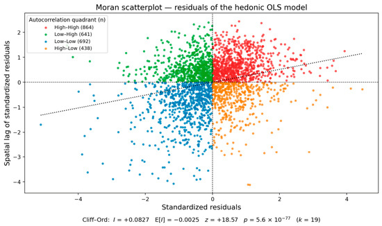
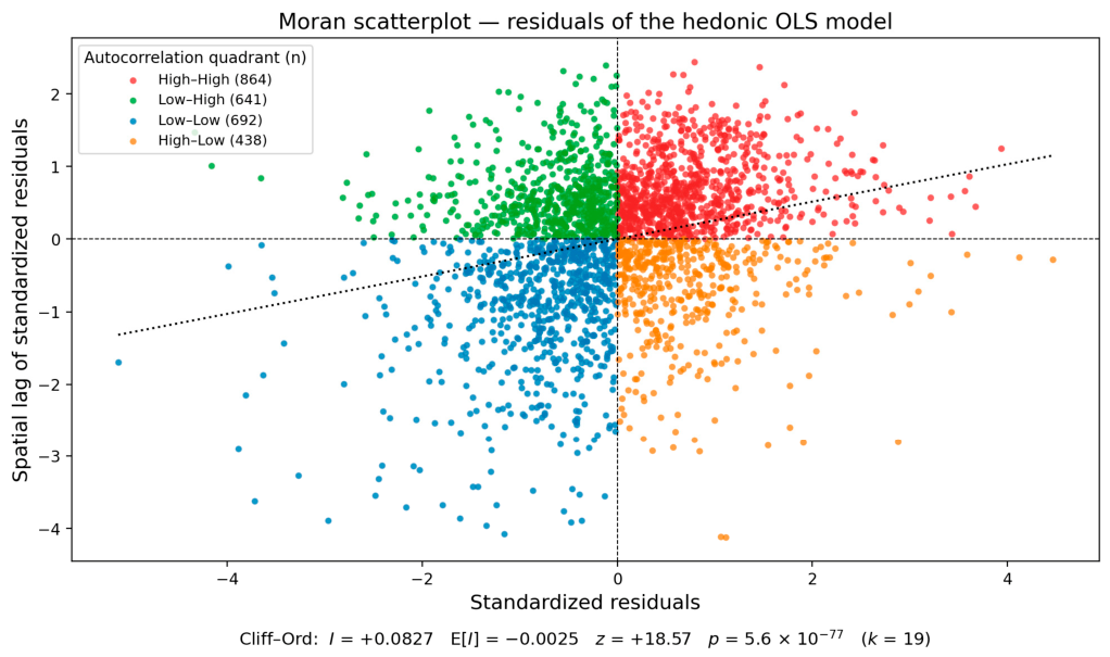
As in the exploratory analysis of the dependent variable, spatial autocorrelation is present in this model’s residuals. Moran’s I, tested against the Cliff–Ord null hypothesis of Section 2.9 with k = 19, yields I = +0.083 against an expectation of −0.003, so z = +18.6, and the null hypothesis of no residual spatial autocorrelation is rejected at any conventional level (Section 3.7).

Figure 6 confirms the spatial dependence of the residuals through the slope of the dotted regression line, indicating positive spatial autocorrelation. This suggests that similar residual values cluster spatially, violating the assumption of spatial independence in classical regression.

Figure 6. Moran scatterplot for the residuals of the hedonic OLS model, with the diagnostic evaluated against the Cliff–Ord null hypothesis (Section 2.9). The dotted line is the fitted slope, and the counts in the legend give the number of parcels in each quadrant. Source: Developed by the authors.

3.3. Classical Spatial Model Results

The three classical specifications of Section 2.5 were estimated on the same 18 hedonic explanatory variables and the same Box–Cox transformation of the response used by the filtered models. On the full sample, the spatial parameter is significant in every specification: the spatial autoregressive model gives $\widehat{\rho }$ = 0.398 (z = 10.80), the spatial error model gives $\widehat{\lambda }$ = 0.614 (z = 15.14), and the SARAR specification gives $\widehat{\rho }$ = 0.261 (z = 5.10) together with $\widehat{\lambda }$ = 0.323 (z = 5.51). Spatial dependence is therefore present in these data under either parameterization, and neither channel is negligible.

Estimated on the 20 training subsamples of Section 2.8 rather than on the full sample, the parameters are stable and remain significant in all 20 partitions: the mean estimate is 0.363 for the lag parameter of SAR and 0.581 for the error parameter of SEM. At the same time, SARAR gives 0.271 and 0.270 for the lag and error parameters, respectively. The two SARAR parameters are of nearly equal magnitude, so we cannot conclude that spatial dependence in these data is predominantly error-type; both channels are present.

Coefficient tables are not reported for these three models, as they are for the unfiltered and filtered models (Table 2 and Table 3 and Supplementary Table S3), and the reason is interpretative rather than practical. In a lag specification, the estimated coefficient is not the marginal effect of the corresponding variable, because the effect propagates through the spatial multiplier (I − $\widehat{\rho }$W)⁻¹; the coefficients are therefore not comparable with those of the unfiltered and filtered models and reporting them side by side would invite exactly that comparison. The spatial error model is not subject to this objection, since it leaves the conditional mean unchanged and its coefficients are directly comparable with those of Table 2 and Table 3; they are reported as Supplementary Table S2, where all 18 covariates keep the signs of the filtered model. What is comparable is reported: the out-of-sample performance in Table 4, the residual diagnostics in Table 5, and the paired comparison with the filtered models in Section 3.9.

Table 5. Residual spatial autocorrelation under the Cliff–Ord null hypothesis, full sample (n = 2635), 30-nearest-neighbor weights.

Model	k	I (E[I]; SD)	z (p)	Verdict
OLS, hedonic (log response)	19	+0.0839 (−0.0025; 0.0046)	+18.83 (4.2 × 10−79)	rejected (under-filtering)
OLS, hedonic (Box–Cox response)	19	+0.0827 (−0.0025; 0.0046)	+18.57 (5.6 × 10−77)	rejected (under-filtering)
SAR (spatial lag, ML)	20	+0.0188 (−0.0028; 0.0046)	+4.72 (2.4 × 10−6)	rejected (under-filtering)
SEM (spatial error, ML)	20	−0.0032 (−0.0018; 0.0047)	−0.32 (0.749)	not rejected
SARAR (lag and error, GMM)	21	+0.0044 (−0.0025; 0.0046)	+1.49 (0.136)	not rejected
ESF-C1	58	−0.0143 (−0.0130; 0.0039)	−0.31 (0.756)	not rejected
ESF-C1 (log response)	57	−0.0134 (−0.0129; 0.0039)	−0.13 (0.896)	not rejected
ESF-C2	38	+0.0077 (−0.0082; 0.0042)	+3.77 (1.7 × 10−4)	rejected (under-filtering)
ESF-C3	82	−0.0292 (−0.0184; 0.0036)	−3.04 (0.002)	rejected (over-filtering)
RE-ESF	≈115	−0.0294 (−0.0298; 0.0023)	+0.18 (0.855)	not rejected

Notes: k is the number of columns of the design matrix, including the constant; for SAR, SEM, and SARAR, it also counts the spatial parameter. Each diagnostic is reported in two composite columns: the residual statistic with its expectation and standard deviation in parentheses, as I (E[I]; SD), and the standardized statistic with its two-tailed p-value, as z (p). E[I] is the expectation under the null hypothesis of no residual autocorrelation and is negative by construction, its magnitude increasing with k (Section 2.9); the residual statistic must be read against it and not against zero. A negative residual I is therefore not, in itself, evidence of over-filtering. ESF-C1, ESF-C2 and ESF-C3 are defined in Section 2.6. For RE-ESF, the model does not determine the number of parameters, since the spatial component is estimated by shrinkage; the row uses the effective degrees of freedom reported by the estimator (≈114.9). The two extreme conventions give z = −5.85 when the spatial component is charged no degrees of freedom (k = 19) and z = +4.77 when all 150 eigenvectors are charged as fixed effects (k = 169); they reject the null hypothesis in opposite directions, and the value of k at which the sign of z changes is 112.5. The fixed-effects filter diagnostic does not depend on any such convention. The two OLS rows differ only in the response transformation; the hedonic OLS on the Box–Cox response is the benchmark used throughout.

3.4. ESF Results

According to the algorithm described above in Python, 139 eigenvectors were retained by the pre-selection criterion of 0.25·λ₁, where λ₁ is the largest eigenvalue (=1.0746). Subsequently, additional eigenvectors were eliminated using the stepwise procedure previously described. As a result, of the 139 candidate eigenvectors, 39 were retained and incorporated into the regression model, 38 of which are statistically significant at the 5% level; the single exception, EV_76, has p = 0.0527.

Due to space limitations, Table 3 presents only the first two selected eigenvectors (EV_6 and EV_9) among the 39 included in the model. The complete trail of the stepwise procedure, with one row per admitted eigenvector, its eigenvalue, the fit and the residual diagnostic after each step, and the final coefficient of each eigenvector, is provided as Supplementary Table S1.

The ESF model yielded an adjusted coefficient of determination (R²adj) of 0.7079, indicating that about 71% of the variability in the transformed unit land price was explained by the explanatory variables and the spatial component, the second term of Equation (4). All 18 covariates are significant at the 5% level and keep the signs of the unfiltered model of Table 2.

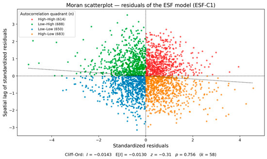
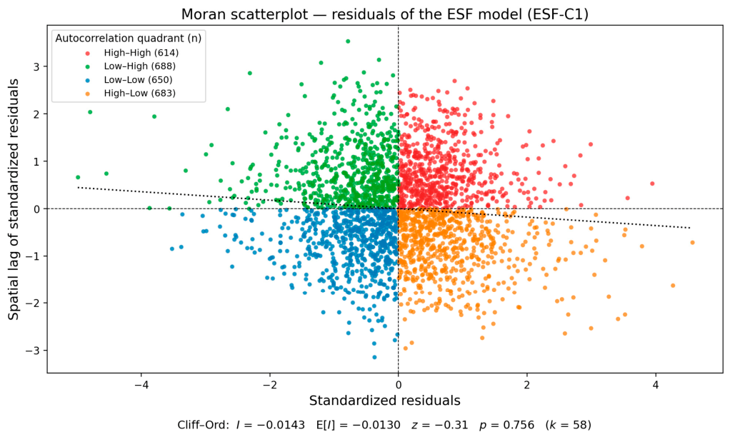
Moran’s I applied to the residuals, tested against the Cliff–Ord null hypothesis of Section 2.9, yielded I = −0.0143 against an expectation of −0.0130 (z = −0.31, p = 0.756; Table 5). The null hypothesis of no residual spatial autocorrelation is not rejected, indicating that the residuals of the ESF model no longer exhibit detectable spatial dependence.

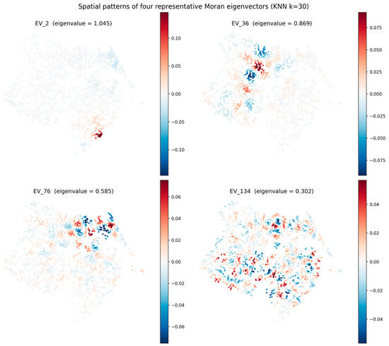
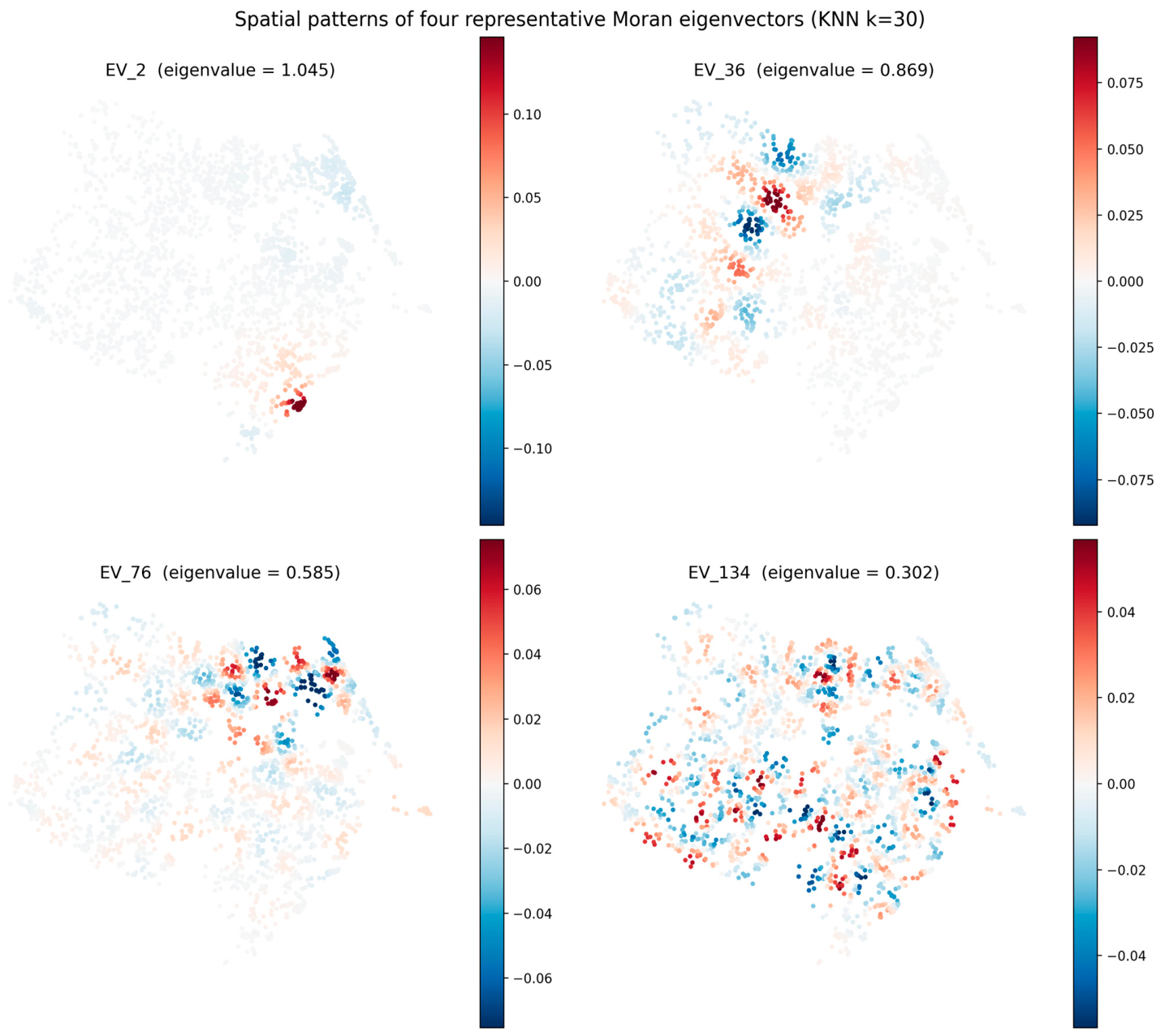
Figure 7 maps four of the 39 selected eigenvectors—at positions 1, 13, 26 and 39 of the set ordered by decreasing eigenvalue—to show the range of spatial scales the filter absorbs: EV_2 (λ = 1.045), EV_36 (0.869), EV_76 (0.585) and EV_134 (0.302). Under a 30-nearest-neighbor matrix, a larger eigenvalue corresponds to a more localized pattern, so EV_2 is the most concentrated of the four and EV_134 the most diffuse. The panels illustrate this multi-scale structure; they are not a ranking of importance, since the stepwise procedure selects eigenvectors by fit, not by eigenvalue order. Confirmation that the residuals are free of spatial autocorrelation is given by the diagnostic in Table 5 and Figure 8.

Figure 7. Spatial patterns of four of the 39 selected Moran eigenvectors, at positions 1, 13, 26 and 39 of the selected set ordered by decreasing eigenvalue: EV_2 (λ = 1.045), EV_36 (0.869), EV_76 (0.585) and EV_134 (0.302). Because the eigenvectors are extracted from the symmetric part of the doubly centered matrix (Section 2.2), each eigenvalue equals the Moran coefficient of its own eigenvector exactly. Under a 30-nearest-neighbor matrix, a larger eigenvalue corresponds to a more concentrated pattern, not to a broader one. The color scale is symmetric and set independently in each panel, bounded at the 99th percentile of the absolute eigenvector values, which clips 27 parcels (1%) per panel. Source: Developed by the authors.

Figure 8. Moran scatterplot for the residuals of the ESF model under ESF-C1. The residual statistic (I = −0.0143) lies essentially on its expectation under the Cliff–Ord null hypothesis (−0.0130), so the hypothesis of no residual spatial autocorrelation is not rejected (z = −0.31, p = 0.76). The dashed lines mark the zero axes, and the dotted line is the fitted slope. Source: Developed by the authors.

3.5. RE-ESF Results

The RE-ESF model was estimated on 150 candidate eigenvectors, the default candidate set in the spmoran package, which differs from the 139 candidates in the fixed-effects filter in Section 3.4. Supplementary Table S3 presents the estimated fixed coefficients of the explanatory variables included in the model, with standard errors in parentheses.

Estimated on the same 18 explanatory variables as the ESF model of Table 3, the RE-ESF specification leaves all 18 covariates significant at the 5% level; only the intercept is not (p = 0.1335), and the least significant covariate is the median house size (acasamed, p = 0.0338). The signs coincide with those of Table 3, including the positive coefficient of the distance to the nearest informal settlement (ln_distassp), and the coefficients are of similar magnitude, with the fixed effects of the source indicators (tr and of) and of the year indicators practically unchanged. The shrinkage estimator retains all 150 candidate eigenvectors, consuming approximately 114.9 effective degrees of freedom, and the estimated standard deviation of the random spatial component is 1.158 on the transformed scale.

Supplementary Figure S2 presents the Moran scatterplot for the RE-ESF residuals. The positive spatial autocorrelation found in the unfiltered model is no longer present. The residual statistic is −0.0294 against an expectation of −0.0298 under the convention of effective degrees of freedom, so that it sits essentially on its expectation and the null hypothesis is not rejected (z = +0.18). The quadrant counts show a predominance of the discordant quadrants, with 731 parcels high–low and 728 low–high against 567 high–high and 609 low–low, an alternating pattern in which a high residual tends to be surrounded by lower ones. This should not be read as negative spatial autocorrelation having emerged: at this number of parameters the expectation of the statistic itself is negative, and the observed value does not depart from it.

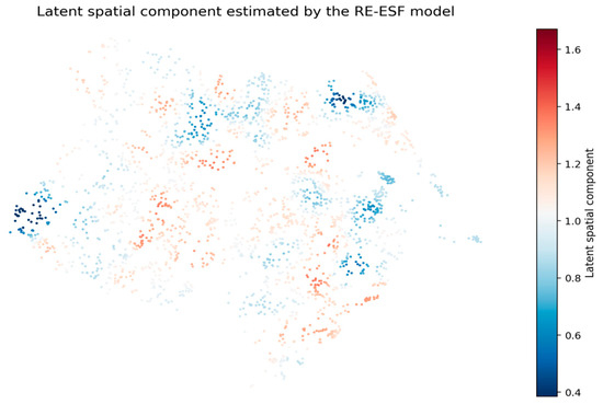
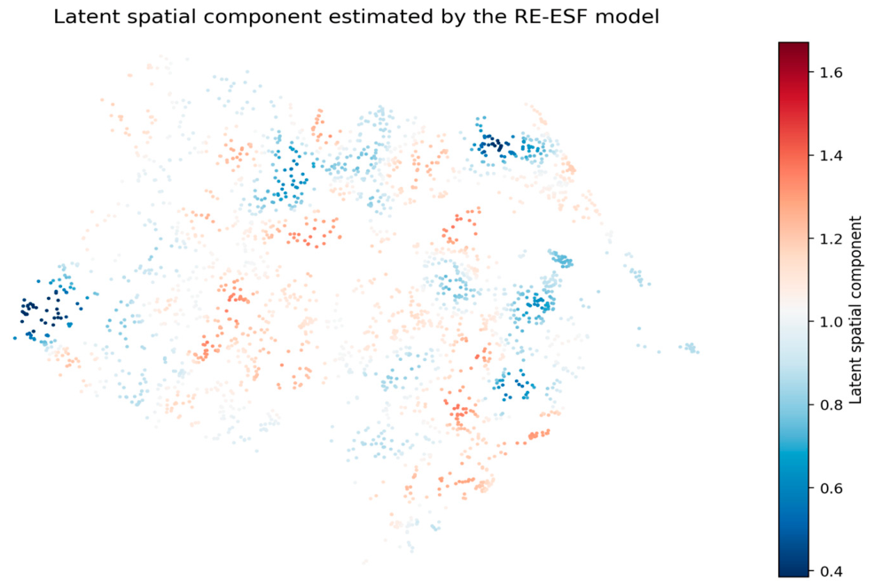
Figure 9 presents the map of the spatial distribution of the latent spatial component estimated by the RE-ESF model. This component represents the locational effects captured by Moran’s eigenvectors, which were extracted and incorporated into the model to correct for spatial autocorrelation not explained by the explanatory variables. Through this map, systematic location-based influences become evident—effects that are not directly observable through traditional covariates but are explicitly modeled through the spatial structure of the RE-ESF approach.

Figure 9. Latent spatial component estimated by the RE-ESF model. The component is strictly positive across the sample, ranging from 0.152 to 1.372 with a median of 1.028. The color scale is symmetric about that median, so that equal color intensity denotes equal deviation from the typical level, and is bounded at the 1^st and 99^th percentiles of the component, which clips 27 parcels (1%). Because the distribution is left-skewed, the upper end of the scale is not reached. Source: Developed by the authors.

The coloring of the points in the map of the latent spatial component (Figure 9) represents the intensity of the locational effects captured by Moran’s eigenvectors. Because the component is strictly positive, ranging from 0.152 to 1.372 with a median of 1.028, the meaningful contrast is not between negative and positive values but between locations below the median (shades of blue, relatively lower prices) and above it (shades of red, prices exceeding what the covariates alone would predict)—pointing to the influence of unobserved locational factors not captured by the explanatory variables.

3.6. Out-of-Sample Validation

Under the design of Section 2.8, the hedonic OLS attains an out-of-sample R² of 0.532 ± 0.053 over the 20 partitions. Both filtered specifications improve on it: ESF-C1 reaches 0.554 ± 0.057 and RE-ESF reaches 0.558 ± 0.058.

The paired comparison drives the conclusion. Against the same hedonic OLS and on the same partitions, ESF-C1 gains 0.0220 in out-of-sample R², outperforming the unfiltered model in 18 of the 20 partitions (Wilcoxon p = 2.7 × 10⁻⁵; paired t-test of the same order), and RE-ESF gains 0.0262, in 19 of 20. Mean absolute percentage error improves in all 20 partitions for ESF-C1, falling from 40.8% to 38.6%.

Two qualifications belong with these figures. First, the gains are small in absolute terms; what supports the conclusion is their consistency across partitions, not their magnitude, and the paired standard deviations reported in Section 2.8 are what make them detectable. Second, the two filtered models are, in practice, tied with each other: the difference between RE-ESF and ESF-C1 is 0.0042 in 13 of 20 partitions (p = 0.058), and RE-ESF has the lower MAPE by 0.19 percentage points in 15 of the 20 partitions, a margin of the same order as the variation between partitions. The defensible distinction between them is parsimony rather than accuracy: 39 eigenvectors entering as fixed effects, against approximately 115 effective degrees of freedom in the random-effects formulation.

The within-sample and out-of-sample orderings do not coincide, and the discrepancy is itself informative. Under ESF-C3, which minimizes the corrected Akaike criterion and retains 63 eigenvectors, the filtered model attains a higher adjusted R² within the sample (0.713 against 0.708) and lower MAPE and MAE, yet it is statistically indistinguishable from ESF-C1 out of sample (difference of 2.7 × 10⁻⁵, p = 0.277). ESF-C2, the most parsimonious of the three with 19 eigenvectors on the full sample, gains 0.0172 in 18 of the 20 partitions, slightly below the other two. The choice of ESF-C1 therefore does not rest on predictive performance; it rests on the residual diagnostic and on parsimony, as Section 3.7 makes explicit.

The result does not depend on the response scale. Estimated with the response in natural logarithms instead of Box–Cox, on the same partitions and against the OLS on the same scale, the filter under ESF-C1 gains 0.0177 in out-of-sample R², in 17 of the 20 partitions (Wilcoxon p = 0.0023), and MAPE improves in all 20. The selected sets are nearly the same: 38 eigenvectors on the logarithmic scale against 39, with 37 in common and the first four admissions identical, and the residual diagnostic is passed on both scales (p = 0.90 in logarithms against p = 0.76 under Box–Cox). Two qualifications go with this. The Box–Cox scale is more favorable in out-of-sample R²: the two unfiltered models are indistinguishable (Table 4), but the filter gains less in logarithms, 0.0177 versus 0.0220. In MAPE, the logarithmic scale is systematically better for the unfiltered model in all 20 partitions and for the filtered one in 18, by about 0.2 percentage points, so the scale adopted does not minimize MAPE. The Box–Cox transformation is inherited from the response specification in Section 2.4 and was not chosen on the basis of these figures.

3.7. Residual Spatial Autocorrelation

Table 5 reports the diagnostics for every model. Measured against the reference of Section 2.9, the hedonic OLS leaves substantial residual spatial autocorrelation: I = +0.083 against an expectation of −0.003, giving z = +18.6 and a p-value below 10⁻⁷⁶. The eigenvector filter removes it. For ESF-C1, I = −0.014 against an expectation of −0.013, so that z = −0.31 and p = 0.76: the residual is indistinguishable from what the null hypothesis predicts. The negative sign of the statistic is expected rather than symptomatic: at k = 58 the reference value is itself negative, more than three standard deviations below zero, so the same statistic, compared with zero, would indicate significant negative autocorrelation. The reference of Section 2.9 removes that artifact.

The same diagnostic discriminates among the eigenvector selection criteria, which is why ESF-C1 was adopted. ESF-C2, which selects by direct reduction in the statistic and is the most parsimonious of those examined at 19 eigenvectors, leaves residual autocorrelation detectable (z = +3.77). ESF-C3, which attains the best within-sample fit with 63 eigenvectors, over-filters: z = −3.04, with the residual statistic significantly below its own expectation. Only ESF-C1 leaves a residual indistinguishable from the null hypothesis while retaining 39 eigenvectors. It was selected on that basis, and not on predictive accuracy, where it ties with ESF-C3.

For the classical specifications, the diagnostic clearly separates the three. The spatial error model removes residual autocorrelation without any eigenvectors (z = −0.32, p = 0.75) and does so in all 20 partitions. SARAR leaves it not significant (z = +1.49, p = 0.14). The spatial autoregressive model does not: z = +4.72 on the full sample, with residual autocorrelation significant in all 20 partitions. A lag in the dependent variable alone therefore does not capture the spatial structure in these data.

For RE-ESF, the test requires a convention, and this should be stated rather than passed over. A shrinkage estimator has no unambiguous number of parameters, so the model does not determine k. Using the effective degrees of freedom that the estimation procedure itself reports (about 115), the residual is indistinguishable from the null hypothesis (z = +0.18, p = 0.86). Treating the spatial component as costing no degrees of freedom (k = 19) or as costing all 150 eigenvectors (k = 169) yields z = −5.85 and z = +4.77, respectively. The two extreme conventions therefore reject the null hypothesis in opposite directions, and the intermediate one lies close to the value of k at which the sign of z changes. The fixed-effects filter diagnostic does not depend on any such convention, which is why ESF is the primary specification in this paper.

3.8. Sensitivity to the Spatial Weights Matrix

Applying the criterion declared in Section 2.10, the conclusions are robust to the specification of the weights matrix. Table 6 reports the five matrices. The filtered model outperforms the hedonic OLS in the paired comparison under each matrix, with out-of-sample R² gains of +0.0142 to +0.0220, winning in 16 to 18 of the 20 partitions, and MAPE improving in all 20 partitions under all five, from 40.8% to between 38.6% and 39.1%. Within the sample, the residual Moran’s I of the filtered model is not significant under any of the five when tested against its own matrix, against z-values from +16.3 to +18.9 for the unfiltered model. Both branches of the criterion are therefore met.

Table 6. Sensitivity of the ESF results (ESF-C1) to the specification of the spatial weights matrix.

Weights Matrix	Candidates/EV	Adjusted R2	Residual z (p)	R2oos (Mean ± SD)	MAPEoos (%; Mean ± SD)	Δ vs. OLS (Wins; Wilcoxon p)
kNN, k = 10	343/66	0.7234	+1.02 (0.307)	0.5506 ± 0.0550	38.68 ± 2.72	+0.0184 (16/20; 2.6 × 10−4)
kNN, k = 20	195/41	0.7093	+1.75 (0.080)	0.5525 ± 0.0576	38.67 ± 2.61	+0.0204 (17/20; 2.1 × 10−4)
kNN, k = 30, adopted	139/39	0.7079	−0.31 (0.756)	0.5542 ± 0.0569	38.62 ± 2.77	+0.0220 (18/20; 2.7 × 10−5)
kNN, k = 40	111/33	0.7062	−0.91 (0.362)	0.5529 ± 0.0529	38.66 ± 2.67	+0.0207 (18/20; 8.5 × 10−4)
Distance band, 1795 m	60/20	0.6938	+0.15 (0.880)	0.5463 ± 0.0582	39.14 ± 2.62	+0.0142 (18/20; 3.9 × 10−4)

Notes: Five row-standardized matrices are compared: k-nearest-neighbor (kNN) graphs with k = 10, 20, 30, and 40, and a distance band of 1795 m, the smallest radius that leaves no parcel without neighbors. Three columns are composite: “Candidates/EV” gives the number of candidate eigenvectors and the number selected; “Residual z (p)” gives the standardized residual statistic with its p-value; and “Δ vs. OLS (wins; Wilcoxon p)” gives the mean paired difference, the number of partitions won out of 20, and the p-value of the signed-rank test. Candidates are the eigenvectors satisfying the pre-selection threshold of 0.25λ₁, and their number falls with k because the threshold becomes more restrictive; the predictive gain does not follow that decline. Adjusted R², the residual z, and its p-value are within-sample, with each model tested against its own weight matrix; the residual z of the unfiltered hedonic OLS ranges from +16.3 to +18.9 across the five matrices. Δ vs. OLS is the mean paired difference in out-of-sample R² against the hedonic OLS over the same 20 partitions. The MAPE of the hedonic OLS, which does not use the matrix, is 40.78% under every one of them; the filtered model improves on it in all 20 partitions under all five. The robustness criterion was fixed before the analysis (Section 2.10) and is met in both branches. Tested pairwise against k = 30, the values k = 20 and k = 40 are statistically indistinguishable from it: the evidence describes a plateau, not an optimum, and k = 30 is an interior value of that plateau. Two results run against the chosen specification and are part of the finding: k = 10 retains the most eigenvectors and combines the best within-sample fit with the worst out-of-sample performance of the four k-nearest-neighbor matrices, so more eigenvectors worsen prediction; and the distance band, whose neighborhoods range from 3 to 195 parcels, is the only matrix that leaves residual autocorrelation significant when tested against a common reference matrix (z = +5.99, p = 2.1 × 10⁻⁹) despite filtering the structure of its own.

The analysis also shows what the choice of k = 30 is not, and these qualifications are part of the result rather than caveats appended to it. When each alternative is compared with k = 30 in a paired test, k = 20 and k = 40 are statistically indistinguishable from it: the evidence describes a plateau, not an optimum. No objective rule selects k = 30 either, and three plausible rules point in three directions: within-sample fit favors k = 10, out-of-sample performance favors k = 20, and the residual autocorrelation of the unfiltered model decreases monotonically with k. Moreover, the ordering within the plateau is not stable across specifications, which is itself an argument against reading anything into it.

Two further findings deserve mention because they bear on the overfitting question. The smallest neighborhood, k = 10, retains the most eigenvectors (66) and produces the best within-sample fit (adjusted R² of 0.723) together with the worst out-of-sample performance of the four k-nearest-neighbor matrices. More eigenvectors therefore worsen prediction, which is direct evidence on the question of overfitting rather than an assertion about it. The distance band, conversely, is the only one of the five that leaves residual autocorrelation significant when tested against a common reference matrix (I = +0.017, z = +5.99), despite filtering the structure of its own matrix; its neighborhoods are highly unequal, ranging from 3 to 195 parcels with a median of 98, and the resulting eigenvectors do not span the intermediate spatial scales. This supports the k-nearest-neighbor construction. One element of the construction was not varied: the pre-selection threshold of 0.25λ₁ is held fixed across the five matrices, so that the number of candidates falls with k (Table 6), and part of the effect attributed to k is an interaction with that threshold.

The value adopted is therefore best described as an interior point of a plateau: conclusions are stable for k between 10 and 40 and under a distance band, out-of-sample performance is statistically indistinguishable for k between 20 and 40, and k = 30 is an intermediate value in that range rather than an optimum.

3.9. Benchmark Against Classical Spatial Models

The three classical specifications in Section 2.5 were estimated on the same explanatory variables, the same response transformation, and the same 20 partitions, so the comparison is paired rather than a juxtaposition of separately reported figures. Ranked by out-of-sample R², the models of the hedonic specification are: RE-ESF 0.558, ESF-C1 0.554, ESF-C3 0.554, ESF-C2 0.549, SEM 0.539, hedonic OLS 0.532, SARAR 0.525 and SAR 0.518.

In the twelve pairwise comparisons between the four filtered models (ESF-C1, ESF-C2, ESF-C3 and RE-ESF) and the three classical ones, the filtered models prevail, with p-values below 10⁻⁴ against SAR and SARAR in every case, and against SEM of 5 × 10⁻⁵ for RE-ESF, 2 × 10⁻³ for ESF-C1, 4 × 10⁻³ for ESF-C3 and 1.2 × 10⁻² for ESF-C2 (Wilcoxon; the paired t-test gives the same ordering). Two features of this result should be read together with it. The margin is modest in level: 0.020 separates the best classical model from the best filtered one, and the models of the hedonic specification lie within an interval of about 0.041. What sustains the conclusion is therefore the consistency of the paired differences rather than the size of the effect. And the classical models are not uniformly outperformed across partitions: of the 240 pairwise partition-level comparisons, they win 23, of which 16 are SEM, four are SARAR, and three are SAR.

The spatial error model deserves separate comment, because it is a serious competitor on three counts. It is the only classical specification that outperforms the hedonic OLS out of sample (+0.0065, winning 15 of 20 partitions); it is the only one that removes the residual spatial autocorrelation without recourse to eigenvectors; and it is the only one that does not require a spatial inverse for prediction. It falls 0.0155 short of ESF-C1 in the paired comparison, winning in five of the 20 partitions. The case for the eigenvector approach against SEM therefore rests on the interpretability of an explicit, mappable spatial component and on the residual diagnostic, not on predictive superiority of any substantial size.

The comparison changes direction when read in MAPE instead of R²oos. Table 4 reports MAPE alongside R²oos for the same 20 partitions: it averages 40.78% for the hedonic OLS and is higher for all three classical specifications—41.06% for SAR, 42.03% for SEM, 41.26% for SARAR—so none of them improves on the baseline by this measure, not even SEM, the only classical specification ahead of OLS in R²oos, which is in fact the worst of the four unfiltered models in MAPE. Every filtered specification lowers MAPE below both the OLS and the three classical models, winning all 20 partitions in every one of the twelve pairwise comparisons. The margin against the classical models (1.8 to 3.7 percentage points) is larger than the margin against OLS itself (1.5 to 2.4 points), because the classical models’ MAPE sits above the baseline rather than below it. R² and MAPE therefore rank the classical models differently: SEM’s edge over OLS is a level-based, R²-specific result that does not carry over to a percentage-error criterion.

Two corrections to the interpretation of the classical models follow from estimating them on this specification. First, the autoregressive parameter of the SARAR does not collapse here: as reported in Section 3.3, its lag and error parameters are of practically equal magnitude, so the dependence cannot be attributed predominantly to either channel. Second, the operational advantage frequently attributed to eigenvector filtering applies to the lag family and not to the classical models as a group: it follows from the spatial inverse that prediction with SAR and SARAR requires, as set out below, and the spatial error model, which predicts through $\mathrm{X}\hat{\mathsf{\beta }}$, is not subject to it at all.

Prediction with SAR and SARAR also evaluates the weight matrix over the test points, so the lag models enter the out-of-sample comparison with information the eigenvector models do not use. This asymmetry works against the argument of this paper, so we quantified it rather than leaving it as a caveat. Predicting with the same estimated parameters but on a graph restricted to training neighbors isolates the channel by which the lag models see test observations: it is worth +0.00064 in out-of-sample R² for SAR and +0.00043 for SARAR, two orders of magnitude below the deficit of about 0.04 against the filtered models, with a standard deviation larger than the mean and the sign reversed in six of the 20 partitions. Removing the advantage therefore makes the classical models slightly worse, which means the conclusion of this section holds against, and not with, the direction of this particular design choice. The measurement isolates that specific channel and does not claim to equalize every conceivable advantage of the reduced form.

The operational advantage of the eigenvector approach concerns the lag family specifically. Prediction with SAR and SARAR requires the reduced form (I − W)⁻¹, and therefore the reconstruction and inversion of the weight’s matrix over the entire set of prediction points. In mass appraisal, where parcels enter the register continuously through subdivision, amalgamation, and cadastral updating, this amounts to an inversion of order n for each newly assessed parcel, so prediction ceases to be a local operation and depends on the whole database. The eigenvector filter estimates its spatial basis once and projects it onto new locations, at the cost of a neighborhood query. This is a property of appraisal engineering rather than statistical fit, and it makes the approach usable for a municipal tax administration, subject to the qualification stated above that the spatial error model is not affected by this constraint either.

4. Conclusions

This study examined Moran’s Eigenvector Spatial Filtering as a means of addressing spatial dependence in urban land prices for mass appraisal at the municipal level. Compared with a hedonic ordinary least squares model estimated on the same explanatory variables and validated on the same partitions, the filtered specification removes the residual spatial autocorrelation that the unfiltered model leaves, the residual statistic becoming indistinguishable from its expectation under the Cliff–Ord null hypothesis and improves out-of-sample accuracy by 0.022 in R², in 18 of the 20 partitions. The improvement is modest in magnitude, and it is its consistency across partitions rather than its size that supports the conclusion.

The random-effects specification performs equivalently, with a gain of 0.026 in 19 of 20 partitions; the two filters are tied in accuracy, and the fixed-effects form is preferred for parsimony, 39 eigenvectors against approximately 115 effective degrees of freedom, and because its residual diagnostic does not depend on a convention for the degrees of freedom.

Three qualifications follow from the design and should accompany any use of these results. The out-of-sample partitions are random rather than spatial, so that test parcels are interspersed among training parcels; the gains reported here are therefore an upper bound on generalization to unsampled areas. The neighborhood size of 30 is an interior value of a plateau rather than an optimum, and no objective rule identifies it. And among the classical specifications, the spatial error model is a close competitor: it removes the residual autocorrelation without eigenvectors and requires no spatial inverse for prediction, so that the case for eigenvector filtering against it rests on the interpretability of an explicit and mappable spatial component, rather than on a large difference in predictive accuracy or on operational grounds, since the spatial error model is not subject to the spatial inverse that the lag models require (Section 3.9), a conclusion reinforced by MAPE, where SEM is in fact the worst of the four unfiltered specifications despite its edge in R².

For mass appraisal, the residual diagnostic is not only a statistical check. Spatially clustered residuals are the mechanism of geographic inequity described in the Introduction: clusters of positive residuals are neighborhoods the model systematically under-assesses, and clusters of negative residuals are neighborhoods it over-assesses, so parcels of equal market value are taxed differently depending on where they lie. The filtered model leaves no such structure, as Table 5 shows, and it lowers the mean absolute percentage error in every partition. In this sense, the contribution to assessment equity is measured rather than assumed: the spatially systematic component of the assessment error is removed.

Two extensions follow from the design. A spatially blocked cross-validation, in which the test parcels form contiguous blocks rather than being drawn at random, would measure generalization to unsampled areas, the situation an administration faces when a newly incorporated district must be assessed, and would be expected to lower the measured performance of every model examined here. Integrating spatial filtering with machine learning methods remains a further avenue for improving predictive performance in practical mass appraisal applications.

References

- Instituto Brasileiro de Avaliações e Perícias de Engenharia [IBAPE]. Norma AMFTPU IBAPE-SOBREA Avaliação. 2024. Available online: https://ibape-nacional.com.br/biblioteca/wp-content/uploads/2024/09/NORMA-AMFTPU-IBAPE-SOBREA_-30-09-2024.pdf (accessed on 30 September 2025).
- Carvalho Junior, P.H.B. Panorama do IPTU: Um Retrato da Administração Tributária em 53 Cidades Selecionadas. 2018. Available online: https://repositorio.ipea.gov.br/bitstream/11058/9313/1/td_2419.pdf (accessed on 29 August 2024).
- De Cesare, C. Condições Básicas para Garantir a Funcionalidade da Tributação Recorrente ao Patrimônio Imobiliário Urbano e Rural. In ANFIP-Associação Nacional dos Auditores-Fiscais da Receita Federal do Brasil [ANFIP]. A Reforma Tributária Necessária: Diagnóstico e Premissas; Plataforma Política Social: São Paulo, Brazil, 2018; pp. 369–393. Available online: https://www.anfip.org.br/?mdocs-file=8605 (accessed on 29 August 2024).
- Oliveira, A.A.F. Tributação Imobiliária: Oportunidades e Desafios. In Escola de Gestão Pública do Estado do Ceará [EGPCE]. Ceará Um Só: Governança Interfederativa em Discussão; Escola de Gestão Pública do Estado do Ceará: Fortaleza, Brazil, 2024; pp. 97–118. [Google Scholar]
- McCord, M.; Lo, D.; Davis, P.; McCord, J.; Hermans, L.; Bidanset, P. Applying the Geostatistical Eigenvector Spatial Filter Approach into Regularized Regression for Improving Prediction Accuracy for Mass Appraisal. Appl. Sci. 2022, 12, 10660. [Google Scholar] [CrossRef] [Scilit]
- Rosen, S. Hedonic Prices and Implicit Markets: Product Differentiation in Pure Competition. J. Political Econ. 1974, 82, 34–55. [Google Scholar] [CrossRef] [Scilit] [PubMed]
- Hu, L.; Chun, Y.; Griffith, D.A. A Multilevel Eigenvector Spatial Filtering Model of House Prices: A Case Study of House Sales in Fairfax County, Virginia. ISPRS Int. J. Geo-Inf. 2019, 8, 508. [Google Scholar] [CrossRef] [Scilit]
- Tobler, W. A Computer Model Simulating Urban Growth in the Detroit Region. Econ. Geogr. 1970, 46, 234–240. [Google Scholar] [CrossRef] [Scilit] [PubMed]
- Anselin, L. Thirty Years of Spatial Econometrics. Pap. Reg. Sci. 2010, 89, 3–26. [Google Scholar] [CrossRef] [Scilit]
- Griffith, D.A.; Chun, Y. Spatial Autocorrelation and Spatial Filtering. In Handbook of Regional Science; Fischer, M.M., Nijkamp, P., Eds.; Springer: Berlin/Heidelberg, Germany, 2013; pp. 1477–1507. [Google Scholar]
- Anselin, L. Spatial Econometrics: Methods and Models; Springer: Dordrecht, The Netherlands, 1988. [Google Scholar]
- Kelejian, H.H.; Prucha, I.R. A Generalized Spatial Two-Stage Least Squares Procedure for Estimating a Spatial Autoregressive Model with Autoregressive Disturbances. J. Real. Estate Financ. Econ. 1998, 17, 99–121. [Google Scholar] [CrossRef] [Scilit]
- Kelejian, H.H.; Prucha, I.R. A Generalized Moments Estimator for the Autoregressive Parameter in a Spatial Model. Int. Econ. Rev. 1999, 40, 509–533. [Google Scholar] [CrossRef] [Scilit]
- Kelejian, H.H.; Prucha, I.R. Specification and estimation of spatial autoregressive models with autoregressive and heteroskedastic disturbances. J. Econom. 2010, 157, 53–67. [Google Scholar] [CrossRef] [Scilit] [PubMed]
- Hastie, T.; Tibshirani, R. Generalized Additive Models; Chapman & Hall: London, UK, 1990. [Google Scholar]
- Rigby, R.A.; Stasinopoulos, D.M. Generalized Additive Models for Location, Scale and Shape. J. R. Stat. Soc. Ser. C (Appl. Stat.) 2005, 54, 507–554. [Google Scholar] [CrossRef] [Scilit]
- Fotheringham, A.S.; Brunsdon, C.; Charlton, M. Geographically weighted regression: A natural evolution of the expansion method for spatial data analysis. Environ. Plan. A 1998, 30, 1905–1927. [Google Scholar] [CrossRef] [Scilit]
- Griffith, D.A. Spatial Filtering. In Spatial Autocorrelation and Spatial Filtering: Gaining Understanding Through Theory and Scientific Visualization; Advances in Spatial Science; Springer: Berlin/Heidelberg, Germany, 2003; pp. 91–130. [Google Scholar]
- Islam, M.D.; Li, B.; Lee, C.; Wang, X. Incorporating Spatial Information in Machine Learning: The Moran Eigenvector Spatial Filter Approach. Trans. GIS 2022, 26, 902–922. [Google Scholar] [CrossRef] [Scilit]
- Hu, L.; Chun, Y.; Griffith, D.A. Incorporating Spatial Autocorrelation into House Sale Price Prediction Using Random Forest Model. Trans. GIS 2022, 26, 2123–2144. [Google Scholar] [CrossRef] [Scilit]
- Griffith, D.A.; Peres-Neto, P.R. Spatial modeling in ecology: The flexibility of eigenfunction spatial analyses. Ecology 2006, 87, 2603–2613. [Google Scholar] [CrossRef] [Scilit]
- Strang, G. Introduction to Linear Algebra, 6th ed.; Wellesley-Cambridge Press: Wellesley, MA, USA, 2023. [Google Scholar]
- Instituto Brasileiro de Geografia e Estatística [IBGE]. Censo Demográfico 2022: População e Domicílios-Primeiros Resultados. 2023. Available online: https://www.ibge.gov.br/estatisticas/sociais/saude/22827-censo-demografico-2022.html (accessed on 29 August 2024).
- Murakami, D. spmoran: An R package for Moran’s eigenvector-based spatial regression analysis. arXiv 2017, arXiv:1703.04467. [Google Scholar]
- Chun, Y.; Griffith, D.A.; Lee, M.; Sinha, P. Eigenvector Selection with Stepwise Regression Techniques to Construct Eigenvector Spatial Filters. J. Geogr. Syst. 2016, 18, 67–85. [Google Scholar] [CrossRef] [Scilit]
- Murakami, D.; Griffith, D.A. Eigenvector Spatial Filtering for Large Data Sets: Fixed and Random Effects Approaches. Geogr. Anal. 2019, 51, 23–49. [Google Scholar] [CrossRef] [Scilit]
- Davidson, R.; Mackinnon, J.G. Estimation and Inference in Econometrics; Oxford University Press: New York, NY, USA, 1993. [Google Scholar]
Disclaimer/Publisher’s Note: The statements, opinions and data contained in all publications are solely those of the individual author(s) and contributor(s) and not of MDPI and/or the editor(s). MDPI and/or the editor(s) disclaim responsibility for any injury to people or property resulting from any ideas, methods, instructions or products referred to in the content. |
© 2026 by the authors. Licensee MDPI, Basel, Switzerland. This article is an open access article distributed under the terms and conditions of the Creative Commons Attribution (CC BY) license.