


Abstract
Efficient structural health monitoring requires not only robust computational strategies but also reliable data acquisition systems capable of capturing representative dynamic responses of real structures. In this study, a continuous dynamic monitoring system composed of accelerometers strategically distributed along the bridge deck provides the foundational data for all subsequent computational analyses. The integrated application of t-Distributed Stochastic Neighbor Embedding (t-SNE) and Learning Vector Quantization (LVQ) is evaluated for the identification of structural damage in the Infante D. Henrique Bridge, located in Porto, Portugal. Data obtained from five years of continuous monitoring were used, with a portion of the identified natural frequencies employed for training and validation of the LVQ algorithm. The robustness of the approach was assessed through artificial modification of data from the second year of monitoring, simulating different damage scenarios. The results demonstrate that the t-SNE–LVQ combination improves discrimination between normal and damaged structural states, achieving identification rates above 70%. The main contribution of this work lies in demonstrating the feasibility and effectiveness of an integrated hardware-to-software machine learning framework applied to real monitoring data, highlighting its potential for structural health monitoring and decision-support systems.
1. Introduction
Structural health monitoring (SHM) has evolved significantly with the use of techniques based on dynamic parameters, enabling the detection of changes in the behavior of structures in operation. However, the identification of low-intensity damage remains a challenge, since small variations in modal parameters may be masked by residual noise and operational variability, especially in real-world datasets [1,2,3,4,5].
In this context, structural damage detection has increasingly been addressed by the scientific community as a pattern recognition problem, in which different structural states are identified based on parameters sensitive to physical changes in the system. Machine Learning techniques have been widely employed for this purpose, as demonstrated in studies by [6,7,8,9,10,11,12,13,14,15,16]. However, many studies focus on complex models or extensive feature sets, which may compromise interpretability and computational efficiency, particularly in continuous monitoring applications using real data.
In SHM applications, the reliability of machine learning-based damage identification depends fundamentally on the monitoring system from which the data are obtained. In the case of continuous dynamic monitoring of bridges, the use of accelerometers distributed along the deck enables the identification of global vibration modes over long observation periods. This sensor configuration is particularly relevant for capturing the natural frequencies adopted in this study. As a result, the proposed computational strategy is intrinsically linked to the underlying acquisition system, forming a hardware-to-software pipeline in which sensing, modal identification, and pattern recognition are sequentially and physically connected.
An alternative approach to address this challenge is the combination of dimensionality reduction techniques with similarity-based classifiers. Although primarily designed as a visualization tool, t-Distributed Stochastic Neighbor Embedding (t-SNE) has proven effective in preserving neighborhood relationships among samples in high-dimensional spaces, thereby enhancing the separation of patterns associated with different structural states. Despite its widespread use in exploratory data analysis and visualization, the integration of t-SNE [17] with supervised classification algorithms, particularly prototype-based methods such as Learning Vector Quantization (LVQ), remains relatively underexplored in the SHM literature, especially in applications involving experimental data from real structures.
LVQ exhibits characteristics that are particularly relevant for detecting subtle damage, including low sensitivity to noise, reduced computational cost, and the ability to discriminate closely spaced classes in the feature space through representative prototype vectors. Furthermore, the exclusive use of natural frequencies as input features, although recognized as less sensitive in certain damage scenarios, allows for an objective evaluation of the proposed method’s ability to identify structural anomalies using globally available information that is widely employed in real SHM systems.
Within this framework, this study evaluates the integration of t-SNE and LVQ for structural damage identification in the Infante D. Henrique Bridge, using real continuous monitoring data. The main contribution of this work lies in demonstrating the feasibility of this integrated approach for detecting small structural anomalies, highlighting its potential as an efficient, interpretable, and computationally viable tool for SHM applications.
2. Methodology
This study proposes an approach for damage identification in structural health monitoring based on the combination of a dimensionality reduction technique and an intelligent supervised classification method. Continuous monitoring data from the Infante D. Henrique Bridge were used, consisting of the first 12 natural frequencies obtained from vibration measurements over a two-year period. Environmental and operational effects were previously removed in [18] using the DynaMo software, so that the modal parameters predominantly reflected the structural behavior. As no real damage was observed during the analyzed period, artificial damage scenarios were simulated by applying correction coefficients to the experimental frequencies, calculated based on a validated numerical model with localized stiffness reductions.
To address the small variations between intact and damaged states, the t-SNE technique was applied to analyze the similarity among frequency patterns and to assist in selecting the most informative combinations. Subsequently, this information was used to train and test an LVQ neural network, which performs classification based on a reduced set of representative patterns. The model’s performance was evaluated using data independent from those employed during training, allowing its generalization capability to be verified. The adopted methodology (Figure 1) presents low computational cost, robustness to noise, and adequate sensitivity for distinguishing between intact and slightly damaged structural states.
Figure 1.
Methodological steps.
2.1. Infante D. Henrique Bridge and Continuous Dynamic Monitoring System
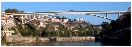
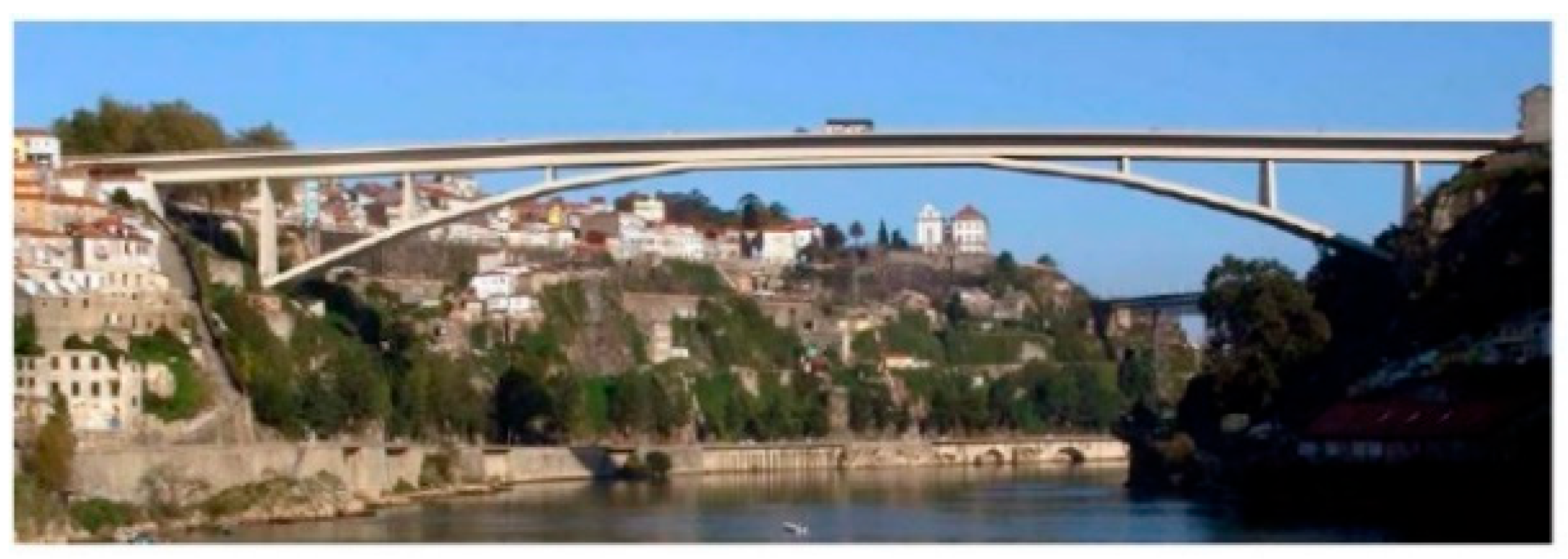
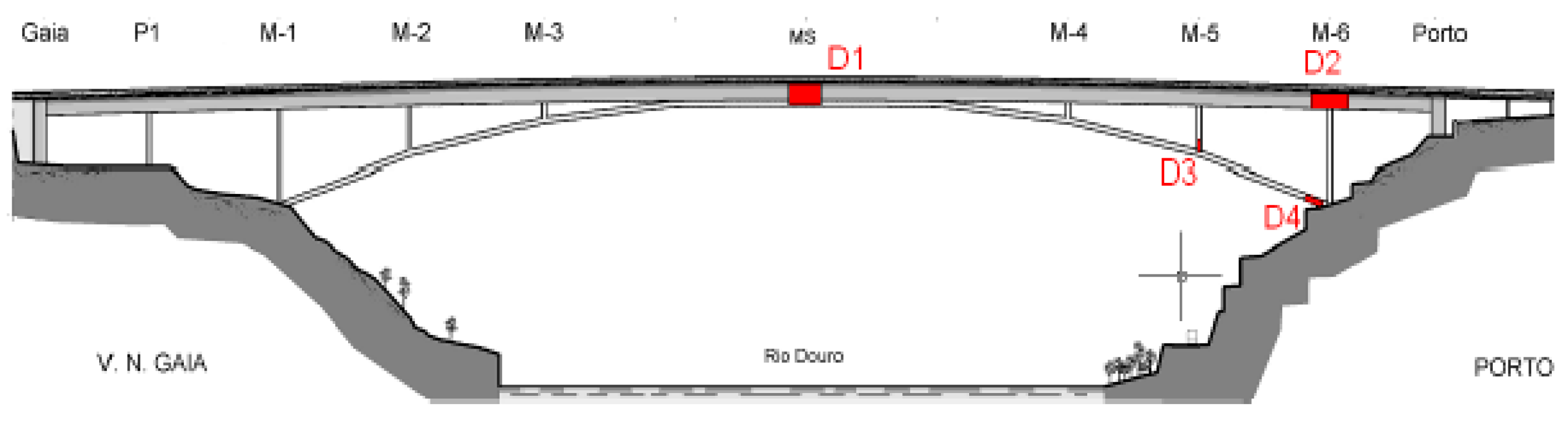
In this study, data from the monitoring system of the Infante D. Henrique Bridge, located over the Douro River and connecting the cities of Porto and Vila Nova de Gaia in Portugal, were used. The bridge, inaugurated in 2003, is a prestressed concrete structure with a total length of 371 m, consisting of two main elements: a rigid box girder made of prestressed concrete, 4.50 m in height, supported by a concrete arch with a thickness of 1.50 m and a span of 280 m (Figure 2).
Figure 2.
Infante D. Henrique Bridge.
The monitoring system was developed and implemented by the Vibrations and Monitoring Laboratory (ViBest) of the University of Porto [19], as part of a continuous structural monitoring study designed to continuously record structural accelerations (vertical, transverse, and longitudinal) through a set of accelerometers distributed along the bridge deck, allowing the consistent identification of global vibration modes and the natural frequencies adopted in this study.
The sensors were connected to digitizers responsible for acquiring the signals and transmitting the data to the Faculty of Engineering of the University of Porto (FEUP). Measurements were carried out automatically, with a sampling rate of 50 Hz and 30 min time intervals, resulting in a long-term observation database. Further information regarding data acquisition can be found in [19].
The files obtained were processed using the Dynamic Monitoring DynaMo software, developed by ViBest [18], which is capable of filtering and cleaning the signals, attenuating environmental and operational effects, and automatically identifying the modal parameters of the structure. At the end of the processing, the extracted natural frequencies and vibration modes were stored in a database that served as a reference for the analyses conducted in this study.
2.1.1. Bridge Monitoring
The continuous monitoring of the Infante D. Henrique Bridge was carried out from 13 September 2007 to 12 November 2012. However, for this study, the data corresponding to the period from 2007 to 2009 were used, totaling approximately 17,500 acquisitions per year.
Aiming at detecting small structural anomalies without the influence of environmental or operational effects, the data used in this study had already been processed by the DynaMo software. This program uses advanced statistical procedures, based on Multiple Linear Regression, to model and remove components associated with temperature variation and other external factors, resulting in modal parameters that more accurately reflect the dynamic behavior of the structure.
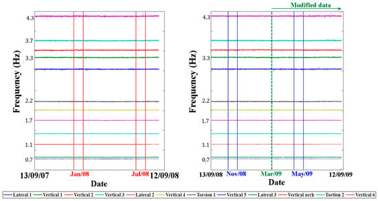
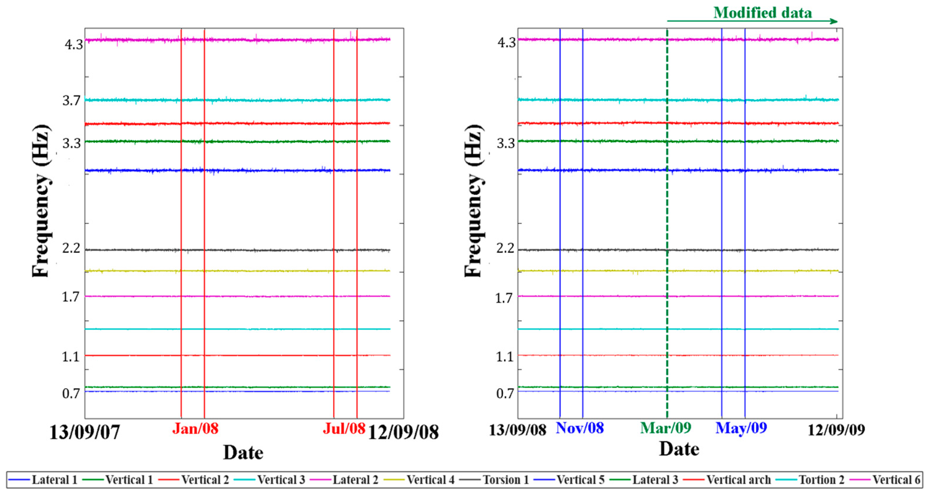
After eliminating environmental and operational effects, Figure 3 shows the chronological evolution of the daily average of the first 12 natural frequencies of the bridge, obtained during the monitoring period considered in this study—first year (13 September 2007 to 12 September 2008) and second year (13 September 2008 to 12 September 2009)—and subsequently used in the analyses performed.
Figure 3.
Time evolution of the bridge’s first 12 natural frequencies from 13 September 2007 to 12 September 2009.
From Figure 3, it can be observed that the first 12 natural frequencies of the bridge vary approximately between 0.7 and 4.3 Hz, with no significant differences between the analyzed periods. It is noted that the vertical markings in red, blue, and green indicate specific periods of data usage, which will be discussed and detailed in Section 2.4.
2.1.2. Simulation of Artificial Damage Scenarios
Considering that during the monitoring period the Infante D. Henrique Bridge did not exhibit significant structural anomalies, the study by [18] sought to understand the potential impact of damage on the modal parameters. For this purpose, a numerical model was developed and validated using the experimental results. Based on this model, several simulations were performed, ranging from the intact structural condition to four different damage scenarios.
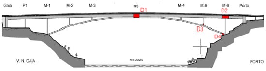
Damage in bridges often manifests in various ways, such as foundation settlement, cable rupture caused by corrosion, concrete pathologies resulting from reinforcement corrosion, among others; therefore, representing them numerically is a challenging task. Accurate numerical modeling of possible damage scenarios, directly motivated by these causes, would require the development of highly complex nonlinear models and the adoption of many assumptions. In this study, a simpler approach was chosen, based on reducing the inertia of regions that may have deteriorated due to aging (Figure 4).
Figure 4.
Schematic layout showing the location and extent of the simulated damage scenarios. Reproduced from [18] (Magalhães, 2010), with permission.
Thus, damage scenarios D1 to D4 were simulated considering a 10% reduction in vertical bending inertia in the bridge segments shown in Figure 4, with lengths: D1—8.75 m; D2—10.0 m; D3—3.0 m and D4—5.0 m [19]. This type of stiffness variation was also investigated by other researchers, such as ref. [19].
It was observed that, as previously mentioned, the impact of the reductions in inertia (stiffness) on the first 12 natural frequencies was not very significant (Table 1). Thus, it was decided to work with the experimental data from the first year considering that they corresponded to the undamaged structure and to modify part of the experimental data from the second year so that they could represent the same damage patterns simulated in the numerical model. To achieve this, correction coefficients were computed based on the relative difference between the numerical frequencies of the intact and damaged models (scenarios D1 to D4). These coefficients were then applied to the experimental frequencies identified in the second year of bridge monitoring in order to simulate different levels of structural damage.
Table 1.
Natural frequencies (Hz) of the intact (experimental) bridge and each of the numerical scenarios.
The coefficient consists of the difference (Δf) between a frequency obtained from the intact numerical model and the frequency of one of the damaged scenarios presented. Thus, to consider that a structural frequency was obtained from one of the damaged scenarios, it is sufficient to multiply it by the following coefficient:
Δfreq → Difference between a frequency from the intact numerical model and the frequency of one of the considered damaged scenarios.
The natural frequencies (Hz) obtained for each damage scenario are presented in Table 1, while the corresponding relative differences (Δf) are shown in Table 2. It is observed that the variations between the intact and damaged models are small, on the order of 0.4%. The small magnitude of the variations poses a challenge for damage detection using natural frequencies, since the presence of noise can mask the analysis. However, as mentioned, the DynaMo software was used to mitigate possible operational and environmental effects in the experimental bridge data
Table 2.
of each of the frequencies, in each damage scenario (numerical).
Finally, in this work, it was assumed that each damage event occurred from 13 March 2009 onwards (dashed green vertical line—Figure 3). From that date, for damage detection testing purposes, the natural frequencies were artificially modified based on the calculated damage coefficients.
2.2. t-Distributed Stochastic Neighbor Embedding (t-SNE)
Dimensionality reduction techniques, such as t-SNE and PCA, have been widely employed in structural health monitoring to address high-dimensional datasets associated with machine learning algorithms [5,20,21,22]. t-SNE, in particular, is a nonlinear method that evaluates data similarity through the formation of clusters in lower-dimensional spaces. In this study, t-SNE was used to guide the training strategy of the LVQ algorithm, enabling the selection of the most representative frequency patterns. Considering the presence of four damage scenarios in addition to the intact state, and the small variations observed in the natural frequencies, this approach allowed for a consistent combination of patterns, reducing redundancies and enhancing class separability.
The method is based on the probability that the proximity between two samples in the high-dimensional space is preserved in the lower-dimensional space. This probability was computed for all points in the high-dimensional space using a normal distribution, represented by , where and denote the -th and -th samples, respectively, and expresses the conditional probability that point identifies point as its nearest neighbor. For points in the lower-dimensional space, neighborhood relationships are described by , obtained from a Student’s t-distribution, which seeks to reproduce the same relationships observed in the high-dimensional space. In the subsequent step, the divergences between the two probability distributions were computed through the algorithm’s cost function (C) and, by means of a gradient-based optimization function, are updated at each iteration until minimized, thereby preserving the original similarity relationships.
2.3. Learning Vector Quantization (LVQ)
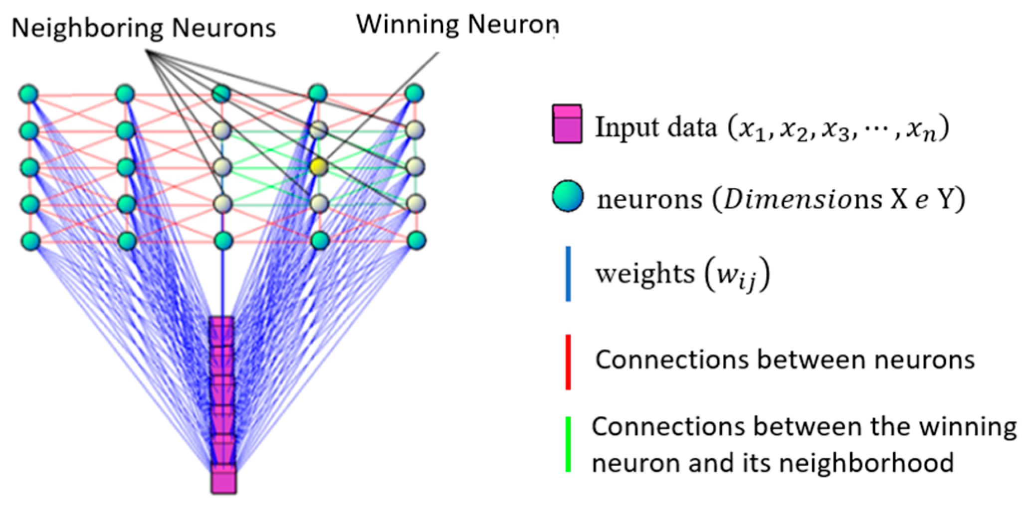
The Learning Vector Quantization (LVQ) algorithm was employed in this study as the final stage for structural state classification. Although supervised, LVQ is derived from Self-Organizing Maps (SOM), combining unsupervised competitive organization with supervised adjustment based on labeled data. LVQ represents each class by a reduced set of reference vectors, and classification is performed (winning neuron −(Figure 5)) based on the minimum distance between the input vector and these reference vectors.
Figure 5.
Structure of the SOM network or Kohonen map.
This strategy is particularly suitable for damage detection problems based on natural frequencies, in which the variations associated with damage presence are small and often affected by residual noise [23]. Unlike methods that use all training samples for decision-making, LVQ relies on a limited number of representative vectors per class, which reduces sensitivity to local fluctuations and increases classification stability in long-term datasets.
During training, the reference vectors were adjusted in a supervised manner, being moved closer to correctly classified patterns and farther away from those associated with incorrect classes, according to
where is the learning rate and is the neighborhood function.
This mechanism enhances the separability between structural states that are very close in the feature space, such as intact and slightly damaged conditions. Moreover, the low computational cost of LVQ and its compatibility with dimensionality reduction techniques, such as t-SNE, make the algorithm suitable for continuous structural health monitoring applications, in which efficiency, robustness, and stability are essential requirements.”
2.4. Damage Detection Using LVQ
Damage detection with LVQ was performed using [24] via the Neural Network Toolbox (Nntool). As it is a supervised training algorithm, LVQ processing begins with specifying the data to be used at each stage: the input and output patterns during training and the test variables corresponding to the problem to be solved.
In this study, each sample corresponds to a data acquisition—that is, a vector containing the 12 natural frequencies obtained from monitoring the structure, both in its intact condition and with artificially simulated damage.
Four frequency patterns obtained from the artificially damaged structure (D1, D2, D3, and D4) were used, which showed variations due to the presence, location, and severity of the damage, as well as two frequency patterns obtained from the information collected during the first and second years of monitoring, assumed to correspond to the intact structure. Each sample consisted of 12 frequencies (obtained in each acquisition, every 30 min), and the patterns were formed by samples collected during the reference months indicated in Figure 3.
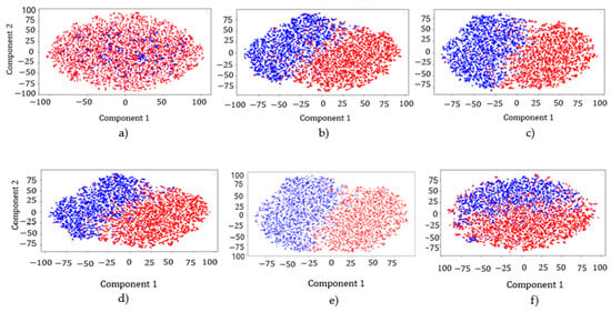
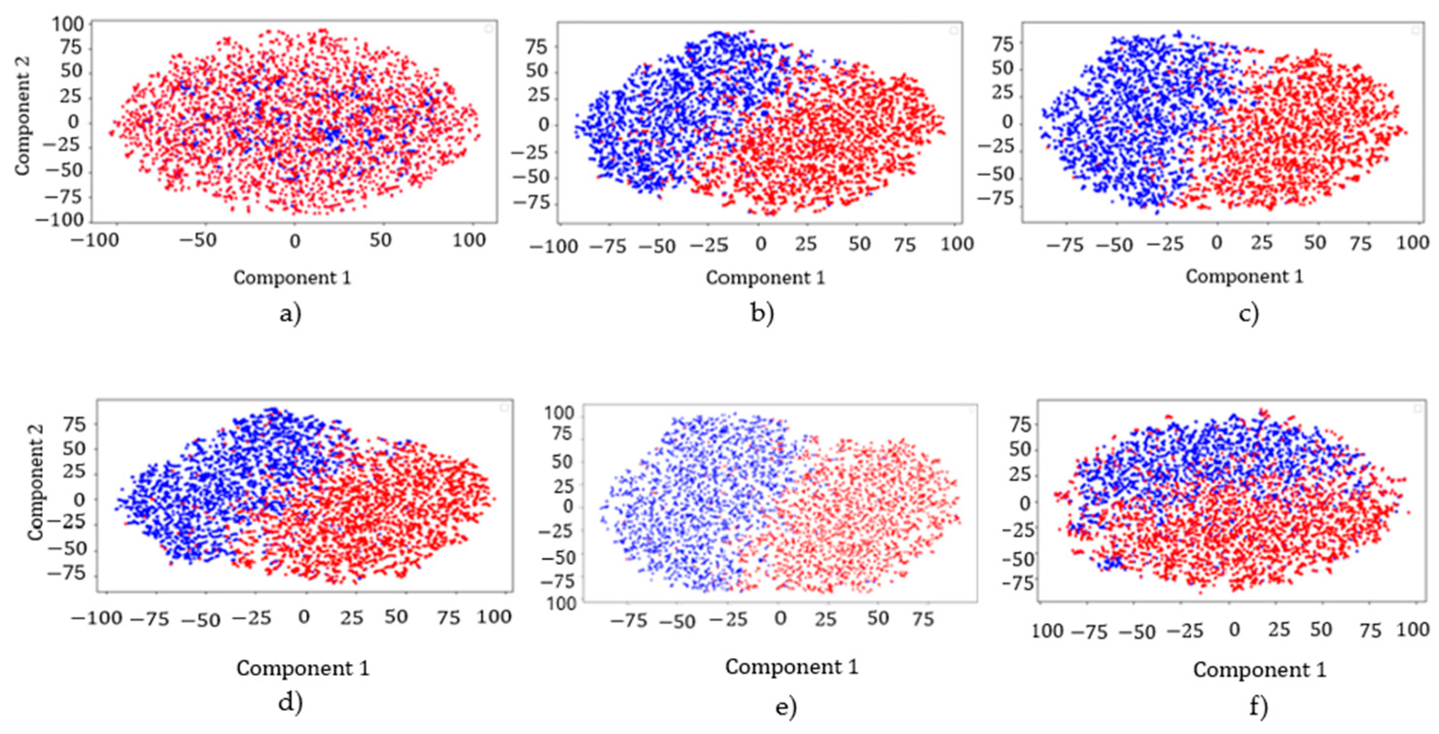
Due to the low amplitude of the variations among the analyzed patterns, the t-Distributed Stochastic Neighbor Embedding (t-SNE) dimensionality reduction technique was applied to evaluate the relationship and degree of separability between the intact and damaged models. This analysis made it possible to identify combinations of frequencies that exhibited similar behavior after the introduction of damage, assisting in defining the best training strategy for the neural network. The t-SNE perplexity was defined within the range recommended in the literature (5–50) and, after preliminary tests, a value of 10 was adopted, as it ensured an adequate balance between the preservation of local and global data structures. The learning rate was kept at the default value defined by scikit-learn, which depends on the number of samples, ensuring stability during the optimization process. The results are presented in Figure 6.
Figure 6.
Frequency patterns relating to damage scenarios D1, D2, D3, and D4: (a) Comparison of frequencies D1 and D2. (b) Comparison of frequencies D1 and D3. (c) Comparison of frequencies D1 and D4. (d) Comparison of frequencies D2 and D3. (e) Comparison of frequencies D2 and D4. (f) Comparison of frequencies D3 and D4.
It can be observed that, when analyzing the frequency patterns related to scenarios D1 and D2 (damage on the bridge deck—Figure 6a), there is a mixing of the information, indicating that the frequencies exhibit similar variations. No clear clustering between the data classes is seen, thus suggesting redundancy in the information.
Analyzing the images in Figure 6b, frequencies of scenarios D1 and D3, Figure 6c, frequencies of scenarios D1 and D4, (d) Frequencies D2 and D3 and (e) Frequencies D2 and D4, a clear class separation can be observed through the formation of clusters. This indicates that dimensionality reduction between the patterns is not feasible. Such results may be caused by the location and severity of the damage in the bridge model, which affects certain vibration modes more significantly.
In the case of Figure 6f, it was still possible to perceive a grouping of two classes of information, however, presenting disturbances.
Considering that a neural network tends to perform more efficiently when trained with a substantial number of patterns, and based on the information described above, it was concluded that the network would be trained using frequencies from three different patterns. Accordingly, the training was configured with frequencies from one intact pattern, one pattern associated with damage scenarios D1 or D2, and a third pattern representing the damaged models D3 or D4.
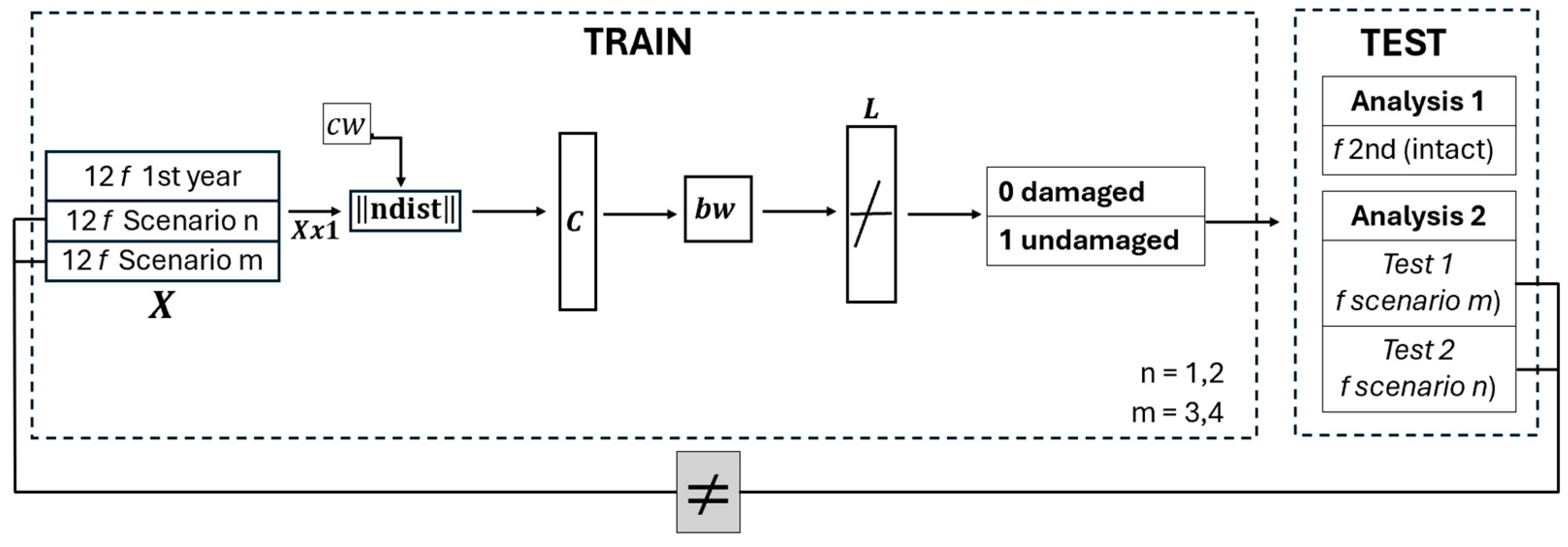
Two types of analyses were performed. The first referred to confirming the intact condition of the structure (for training: frequencies from the first year of monitoring, assumed to represent the intact structure + experimental frequencies from two artificially damaged scenarios), and in the testing phase, the frequencies obtained during the second year of monitoring the structure, without considering any type of modification caused by damage.
In the second analysis group, the training set was the same as in Analysis 1, while the tests were conducted using information from damaged models, excluding those used in training. Therefore, the structural health assessment was approached using two sets of analyses, as detailed in Table 3.
Table 3.
LVQ analyses.
Since LVQ is a supervised learning network, and in this study it was used as a classification system, the ANN output was structured as a two-row matrix containing the numbers 1 and 0, representing the patterns of ‘damaged frequencies’ and ‘intact frequencies, respectively. Figure 7 shows the LVQ network architecture used in this study.
Figure 7.
LVQ performed analyses.
Despite the use of the DynaMo software to minimize environmental effects (caused by thermal variations), residual thermal influences may still be present in the structural data. Therefore, two reference months were selected to train the networks: January and July (indicated by red vertical markers in Figure 3), as they represent periods of large temperature variations in Portugal.
For the testing stage of the method, the frequencies obtained in November 2008 and May 2009 (indicated by blue vertical markers in Figure 3), corresponding to the second year of bridge monitoring, were used.
3. Results
As presented in Table 3, two types of analyses were carried out: the first concerned confirming the bridge in its intact state, while the second analysis referred to damage identification based on the scenarios shown in Figure 4.
3.1. Analysis 1: LVQ Test Using Only Data from a Bridge Considered Intact
Initially, the first 12 frequencies obtained at each acquisition during the first year of structural monitoring were used to train the ANNs. In addition, the artificially modified frequencies representing the damage scenarios D1, D2, D3, and D4 were incorporated. The goal was to evaluate the sensitivity of the LVQ in detecting and distinguishing between frequencies that represent the intact state of the structure and those affected by damage. In this context, the networks were configured according to the specifications presented in Table 3 (Analysis 1).
The networks were built with 15 neurons, and their processing was performed in an average of 100 iterations and errors on the order of 10−2.
As mentioned, LVQ classifies the data provided as input. In this case, since the patterns were learned as two classes (damaged and intact), the following graphs show the results obtained, where the correct classifications refer to the number of samples (the set of frequencies estimated during the second year of monitoring) classified as intact.
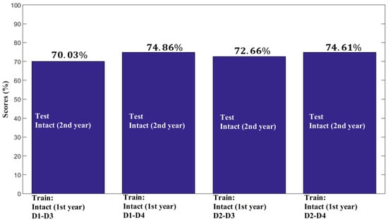
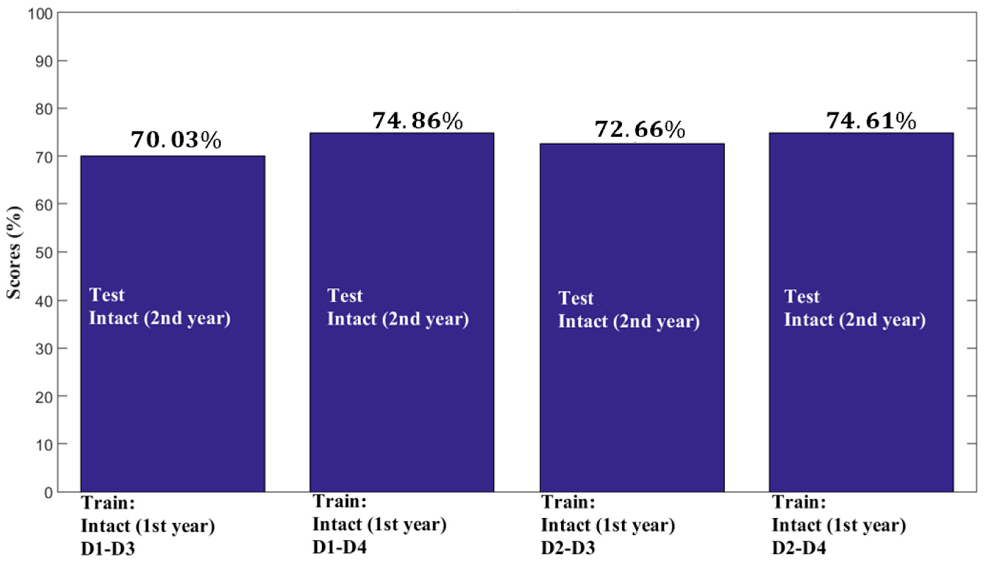
It can be observed that, in all tests of Analysis 1 (Figure 8), the LVQ showed a good accuracy rate, since in all simulations approximately 70% of the frequency sets were correctly classified as corresponding to the intact structure, that is, without indications of changes that could suggest the presence of structural damage in the bridge.
Figure 8.
Results obtained in analysis 1, LVQ.
3.2. Analysis 2: Training and Testing of LVQ with Data from a Bridge Considered Intact and Artificially Damaged
To evaluate the sensitivity of the LVQ to different damaged scenarios, the second analysis was divided into two groups. For each pair of damaged model patterns used in training, the networks were tested with the frequencies of the other two scenarios. All networks had 15 neurons and were trained with an average of 150 iterations, achieving errors on the order of 10−2. The network configurations (input and output) were presented in Table 3 (Analysis 2).
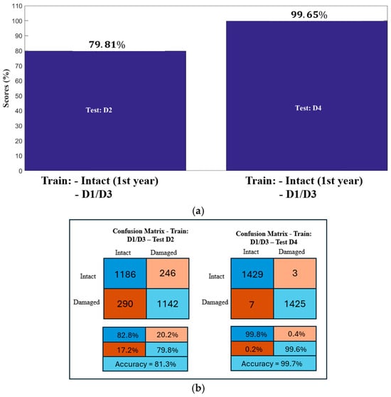
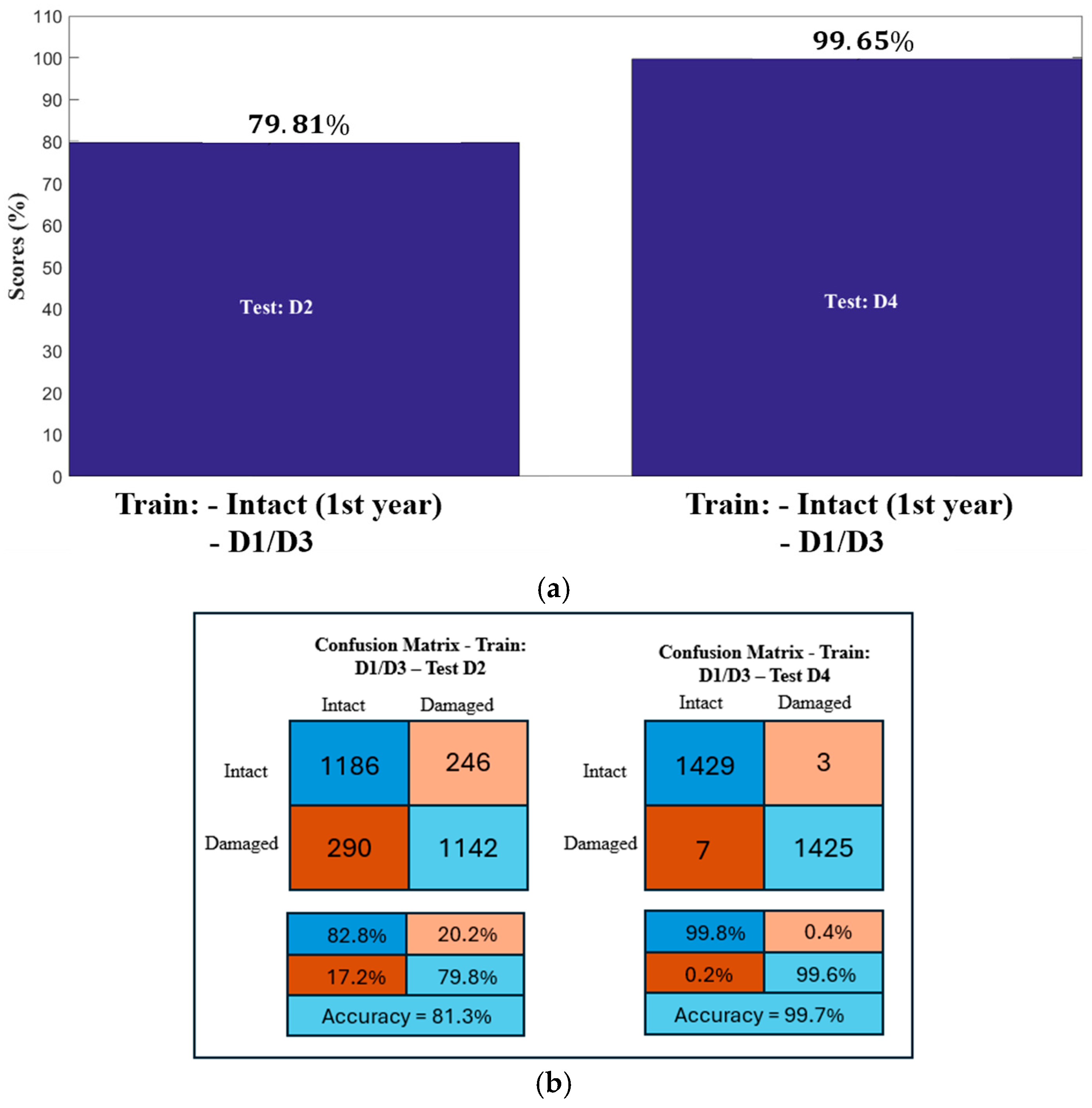
The results of network 1 can be seen in the graphs in Figure 9a. It can be observed that, when trained with the D1–D3 damage patterns and the intact pattern (first year of monitoring), the network was able to correctly classify the tests performed with frequencies from the models containing D2 and D4 damage, achieving accuracy rates of 79.81% and 99.65%, respectively.
Figure 9.
Results obtained in analysis 2 (ANN1)—LVQ: (a) Scores in analysis 2—ANN1. (b) Confusion Matrix—analysis 2 (ANN1).
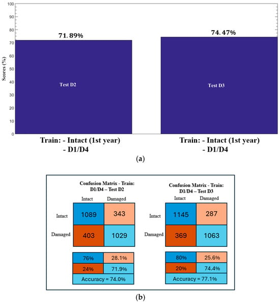
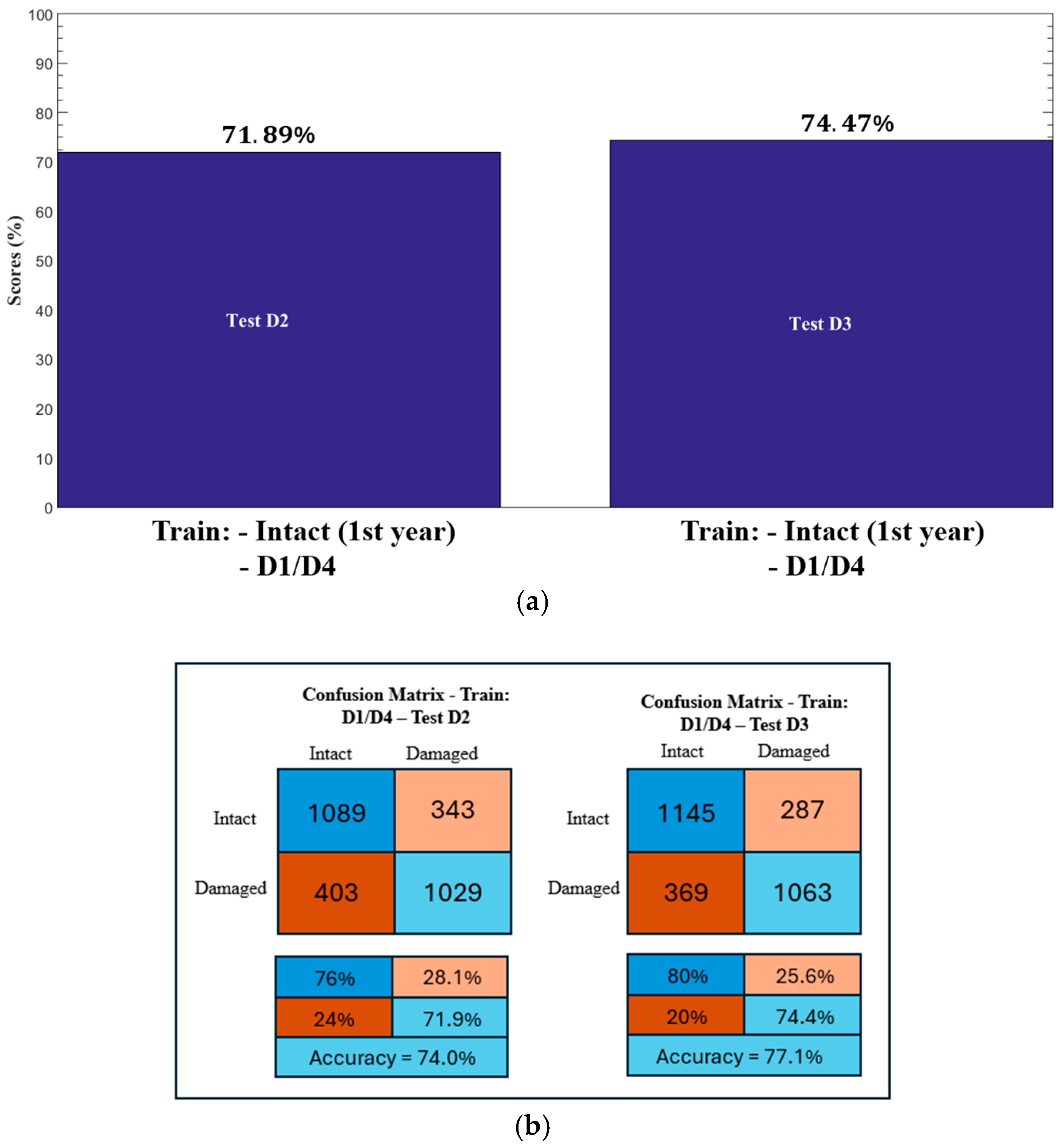
In the case of Network 2 (Figure 10a), the behavior of the algorithm was also satisfactory. The results showed 71.89% accuracy in the D2 test; that is, the network trained with the frequencies estimated during the first year of monitoring (intact), together with the frequencies from the D1 and D4 damage models, was able to distinguish the frequencies from the scenario containing damage 2 (D2) from the frequencies estimated during the second year of continuous bridge monitoring (without damage).
Figure 10.
Results obtained in analysis 2 (ANN2)—LVQ: (a) Scores in analysis 2—ANN2. (b) Confusion Matrix—analysis 2 (ANN2).
In the case of the second test, which evaluates the performance of the LVQ when subjected to testing with the frequencies of the model containing damage corresponding to D3, the algorithm performed properly, achieving approximately 75% accuracy.
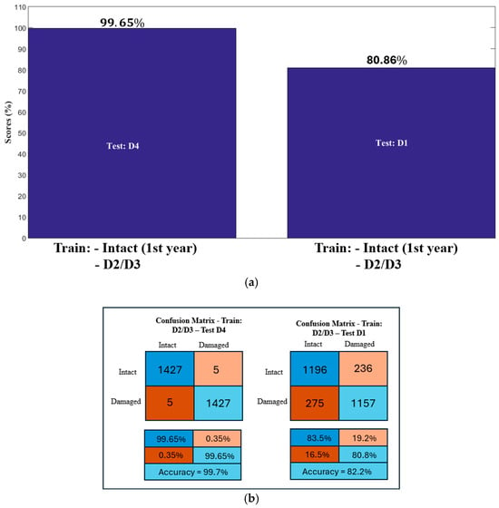
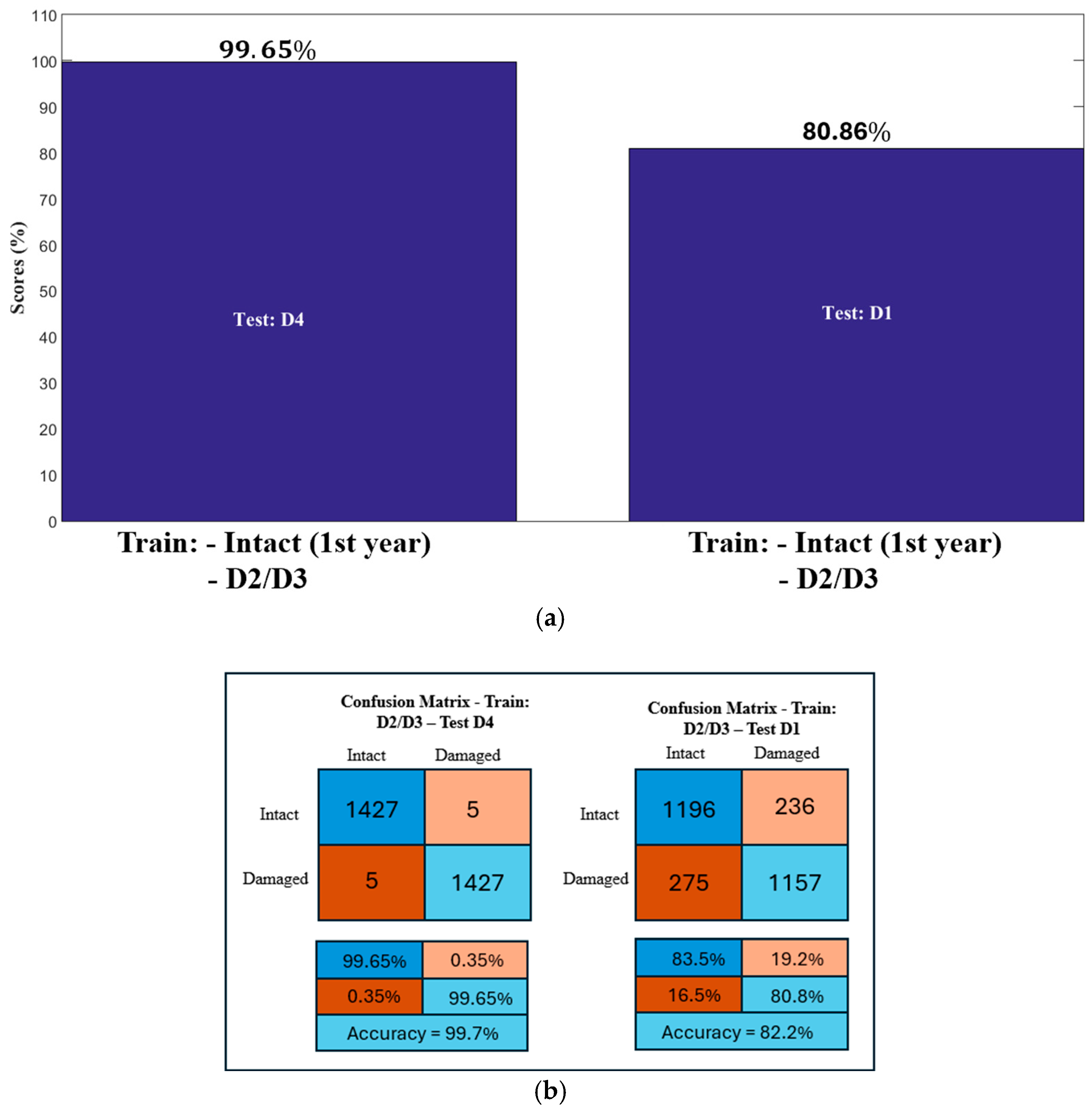
Network 3, configured to be trained with frequencies damaged by D2 and D3, in addition to the frequencies obtained during the first bridge monitoring (intact), was also efficient. In Test 1, considering that the ANN test inputs the frequencies related to the model damaged by the reduction in inertia (D4), the LVQ showed excellent performance, with a 99% accuracy rate (Figure 11a). In other words, when the damaged frequencies from model D4 were provided, almost all sets of the 12 frequencies were classified in the group of damaged frequencies.
Figure 11.
Results obtained in analysis 2 (ANN3)—LVQ: (a) Scores in analysis 2—ANN3. (b) Confusion Matrix—analysis 2 (ANN3).
It can be observed that, when the pattern corresponding to the scenario with damage D4 was used as the test pattern, the results were equal to or greater than 99% (Figure 9a and Figure 11a). This can be explained by the fact that the damage is located in the arch, primarily affecting vertical frequencies 5 and the vertical frequency of the arch, and therefore differing considerably from the other patterns, as shown in Table 2. It is noticeable that these frequencies exhibit the largest variations when considering the damage in scenario D4.
The same behavior was observed in Test 2 (testing with the frequencies of the damaged D1 model). However, the accuracy level was slightly lower, with a precision of 80%.
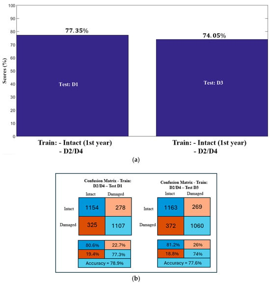
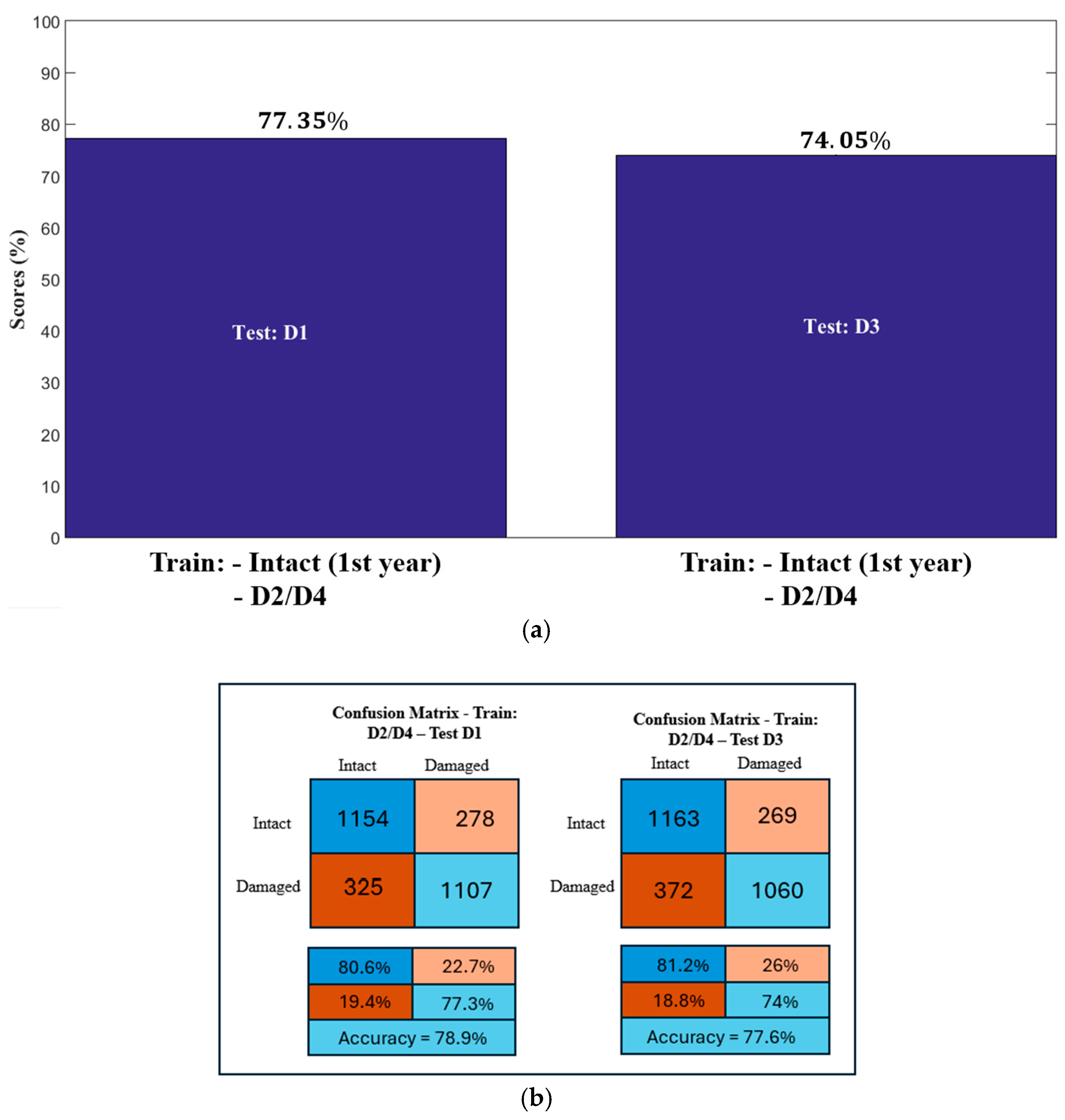
The last network, trained with frequencies corresponding to the D2 and D4 damaged models in addition to the intact model (first year), also followed the performance observed in the earlier rounds. In both tests, it was possible to correctly classify 77.35% of the frequencies from the model damaged with D1 (first test) and 74.05% from the model damaged with D3 (Figure 12a).
Figure 12.
Results obtained in analysis 2 (ANN4)—LVQ: (a) Scores in analysis 2—ANN4. (b) Confusion Matrix—analysis 2 (ANN4).
In summary, an accuracy level above 70% was observed in all analyses performed, which can be considered good results, since similar levels were reported by refs. [25,26,27,28] in an analysis carried out with data from computationally constructed models.
Furthermore, by observing the trends suggested by t-SNE, it is possible to perceive the differences among the D1, D2, D3, and D4 patterns; that is, the algorithm was able to clearly define clusters for each information set, even though some overlap occurred, causing color mixing in certain clustering figures (Figure 6). However, when analyzing specifically the cases comparing the D4 damage pattern with other scenarios, D1 and D2, in Figure 6c,e, a clear separation between the clusters can be observed, indicating greater variation among the information sets. This result was confirmed after processing the ANNs, in which the accuracy levels of Networks 1 and 3 were above 99%.
In a complementary manner, the analysis of the confusion matrices associated with each evaluated case allowed a more detailed interpretation of the LVQ performance, highlighting not only the overall accuracy rates but also the distribution of classification errors between the intact and damaged classes (Figure 9b, Figure 10b, Figure 11b and Figure 12b). It is observed that the best classifier performances coincide with the scenarios in which t-SNE indicated greater separability among the patterns, particularly in cases involving damage D4, where the clusters exhibited larger distances in the reduced-dimensional space. In these cases, the confusion matrices showed a predominance of true positives and true negatives, with low error rates, confirming the LVQ’s ability to generalize and identify damage patterns not used during training. Conversely, in scenarios where t-SNE indicated greater overlap among clusters, a relative increase in misclassifications was observed, which was directly reflected in the confusion matrices and in lower accuracy levels. Thus, the results demonstrate a strong coherence between the exploratory analysis performed by t-SNE and the quantitative performance of the LVQ, indicating that the separability observed in the reduced space is directly associated with the efficiency of the neural classifier in detecting structural damage.
Table 4 summarizes the classification accuracy obtained for the different damage scenarios, confirming the robustness of the proposed framework even for very small frequency variations.
Table 4.
LVQ Classification Accuracy.
Furthermore, it was observed that damage detection based solely on vibration frequency may present uncertainties, since temperature can cause significant variations in this dynamic characteristic, enough to mask the presence of damage, as noted by [29,30].
4. Conclusions
This study explored the performance of LVQ and t-SNE in the detection of structural damage in the Infante D. Henrique Bridge, using a database obtained from continuous structural monitoring. Since no actual damage was observed in the bridge, part of the experimental database was artificially modified to simulate different damage scenarios.
Two analyses were carried out to evaluate the algorithm’s performance. In the first analysis, the ANN was trained with frequencies from the structure considered intact, obtained during the first year of bridge monitoring, together with artificially damaged frequencies generated through numerical models. The test was conducted using frequencies from the second year of monitoring, assumed to be intact. In the second analysis, the training followed the same approach as in the first case, but the test was performed with frequencies artificially modified to represent the presence of four structural damage scenarios.
Based on the results obtained, some considerations regarding the functioning of the technique should be highlighted:
- The application of t-SNE as a preprocessing step proved to be fundamental in the context of structural health monitoring. The visualization of a potential dimensionality reduction helped guide the selection of the most informative frequency patterns, resulting in a more efficient training configuration for the LVQ algorithm. This strategy produced a more compact data representation, directly contributing to an increased ability to discriminate between intact and damaged states.The results indicate that the representations generated by t-SNE enabled the visualization of clusters associated with different damage scenarios, with particular emphasis on the greater separability of scenario D4 compared to the others. This qualitative evidence was consistent with the quantitative performance of the LVQ, which achieved higher accuracy rates in scenarios with clearer visual separation, confirming the coherence between the exploratory analysis and the classification stage.It should be noted, however, that t-SNE has well-known limitations, such as sensitivity to hyperparameter selection and the predominantly local preservation of data relationships, without guaranteeing the maintenance of global distances. These characteristics explain the overlap observed in some scenarios with very similar modal variations. In this study, such limitations did not compromise the results, since t-SNE was used exclusively as an exploratory tool to support the definition of the training strategy, rather than as a direct classification method.Overall, the main contribution of using t-SNE in this work lies in its role as a data-driven filter capable of optimizing the input to the LVQ classifier and enhancing the accuracy of structural diagnosis. Within the SHM framework, this approach contributes to more interpretable, efficient, and robust systems, particularly in applications involving small variations in dynamic parameters.
- The frequencies showed very small variations in the presence of different structural damages when compared to the intact scenarios and among themselves (depending on the damage location). It is possible to verify in Table 1 and Table 2 that only a few frequencies exhibit more noticeable differences. Thus, it becomes clear that the network’s performance is always better when a larger number of variables is available in the samples, as long as they are representative of the problem. In this case, if only the first four frequencies had been used, LVQ would likely not have been able to detect variations significant enough to classify the test dataset as intact or damaged, since Δfreq is nearly 0% (Table 2).
- In addition to a considerable number of variables, attention is drawn to the need to train the network with the widest possible range of data patterns found in structures. In this work, the patterns were defined by damage scenarios at strategic locations, allowing the network to establish the relationship between inputs and outputs over a broad range of possible cases and then correctly classify the inputs. Therefore, it can be indicated that, for this case, the damaged patterns were sufficient, as they included damage in both the deck and the arch. Since the bridge structure is symmetrical, it is expected that if damage occurred on the opposite side, the frequencies would behave similarly.
- In Analysis 2, LVQ achieved accuracy rates between 70% and 99% when identifying damaged patterns not used during the training phase. Networks trained with certain combinations of damages were able to generalize and detect other patterns, reinforcing the model’s extrapolation capability. The best performances were observed in the tests with scenario D4, with accuracies above 99%, which can be attributed to the significant alteration of the vertical frequencies associated with the bridge arch.
- The lack of experimental data containing frequency changes caused by substantial anomalies in the bridge was not considered a negative factor. Some tests were conducted using the second-year monitoring data artificially modified based on previous numerical analyses. It is worth noting that these changes were derived from coefficients obtained from very small damages so as not to compromise the functioning of the structure.
Finally, an adequate performance of the technique was observed, indicating that it may serve as a potential tool to complement structural monitoring systems, especially due to its capacity to process large volumes of data that need to be interpreted more rapidly for structural damage detection. Furthermore, it allows the use of various types of information from the monitored structure. In other words, it does not present limitations regarding the type of structure under analysis. However, although the methodology demonstrated good performance in detecting damage in the Infante D. Henrique Bridge, it should be considered effective only after validation on other structural systems.
Author Contributions
Conceptualization, M.M. and G.D.; methodology, M.M. and G.D.; software, M.M.; validation, M.M. and G.D.; formal analysis, M.M.; investigation, M.M.; resources, G.D.; data curation, M.M.; writing—original draft preparation, M.M.; writing—review and editing, M.M. and G.D.; visualization, M.M.; supervision, G.D.; project administration, G.D. All authors have read and agreed to the published version of the manuscript.
Funding
This research received funding from CNPq (National Council for Scientific and Technological Development, Brazil) and CAPES (Coordination for the Improvement of Higher Education Personnel, Brazil).
Data Availability Statement
Restrictions apply to the availability of these data. Data were obtained from [third party] and are available [Magalhães, F] [18].
Conflicts of Interest
The authors declare no conflicts of interest.
Abbreviations
The following abbreviations are used in this manuscript:
| ANN | Artificial Neural Network |
| t-SNE | t-Distributed Stochastic Neighbor Embedding |
| LVQ | Learning Vector Quantization |
| SOM | Self-Organizing Maps |
| SHM | Structural Health Monitoring |
References
- Pereira, S.; Magalhaes, F.; Gomes, J.P.; Cunha, A.; Lemos, J.V. Dynamic monitoring of a concrete arch dam during the first filling of the reservoir. Eng. Struct. 2018, 174, 548–560. [Google Scholar] [CrossRef] [Scilit]
- Toledo, E., Jr.; Cury, A.; Landre, J., Jr. Assessment of low-cost wireless sensors for structural health monitoring applications. Rev. Ibracon. Estrut. Mater. 2021, 14, e14213. [Google Scholar] [CrossRef] [Scilit]
- Pereira, S.; Magalhaes, F.; Gomes, J.P.; Cunha, A.; Lemos, J.V. Vibration-based damage detection of a concrete arch dam. Eng. Struct. 2021, 235, 112032. [Google Scholar] [CrossRef] [Scilit]
- Avci, O.; Abdeljaber, O.; Kiranyaz, S.; Hussein, M.; Gabbouj, M.; Inman, D.J. A review of vibration-based damage detection in civil structures: From traditional methods to Machine Learning and Deep Learning applications. Mech. Syst. Signal Process. 2021, 147, 107077. [Google Scholar] [CrossRef] [Scilit]
- Atia, A.E.S.M.; Vafaei, M.; Tee, K.F.; Aliah, S.C. A Systematic Review of Structural Health Monitoring Using Artificial Neural Networks: From Traditional Neural Networks to Deep Learning Algorithms (Version 1). Res. Sq. 2024, preprint. [Google Scholar] [CrossRef] [Scilit]
- Elkordy, M.F.; Chang, K.C.; Lee, G.C. Neural networks trained by analytically simulated damage states. J. Comput. Civ. Eng. 1993, 7, 130–145. [Google Scholar] [CrossRef] [Scilit]
- Omenzetter, P.; Lautour, O.L. Nearest neighbor and learning vector quantization classification for damage detection using time series analysis. Struct. Control. Health Monit. 2010, 17, 614–631. [Google Scholar]
- Tibaduiza, D.A.; Mujica, L.E.; Rodellar, J. Damage classification in structural health monitoring using principal component analysis and selforganizing maps. Struct. Control. Health Monit. 2013, 20, 1303–1316. [Google Scholar] [CrossRef] [Scilit]
- Bandara, R.P. Damage Identification and Concition Assessment of Building Structures Using Frequency Response Functions and Neural Networks. Ph.D. Thesis, School of Civil Engineering and Built Environment, Queensland University of Technology, Brisbane, Australia, 2013. [Google Scholar]
- Nick, H.; Ashrafpoor, A.; Aziminejad, A. Damage Identification in Steel Frames Using Dual-Criteria Vibration-Based Damage Detection Method and Artificial Neural Network. Structures 2023, 51, 1833–1851. [Google Scholar] [CrossRef] [Scilit]
- Wang, H.; Barone, G.; Smith, A. Current and future role of data fusion and machine learning in infrastructure health monitoring. Struct. Infrastruct. Eng. 2024, 20, 1853–1882. [Google Scholar] [CrossRef] [Scilit]
- Santos-Vila, I.; Soto, R.; Vega, E.; Crawford, B.; Peña, A. Damage Detection on Real Bridges Using Machine Learning Techniques: A Systematic Review. Appl. Sci. 2025, 15, 8884. [Google Scholar] [CrossRef] [Scilit]
- Ahmed, M.S. Detecção de Danos em Lajes Quadradas de Concreto Reforçado Utilizando Análise Modal e Rede Neural Artificial. Tese de Doutorado em Filosofia. Ph.D. Thesis, Nottingham Trent University, Nottingham, UK, 2016. [Google Scholar]
- Gomes, G.F.; Mendez, Y.A.D.; da Silva Lopes Alexandrino, P.; da Cunha, S.S., Jr.; Ancelotti, A.C., Jr. A Review of Vibration Based Inverse Methods for Damage Detection and Identification in Mechanical Structures Using Optimization Algorithms and ANN. Arch. Comput. Methods Eng. 2019, 26, 883–897. [Google Scholar] [CrossRef] [Scilit]
- Jayasundara, N.; Thambiratnam, D.P.; Chan, T.H.T.; Nguyen, A. Damage detection and quantification in deck type arch bridges using vibration based methods and artificial neural networks. Eng. Fail. Anal. 2020, 109, 04265. [Google Scholar] [CrossRef] [Scilit]
- Scarselli, G.; Nicassio, F. Machine Learning for Structural Health Monitoring of Aerospace Structures: A Review. Sensors 2025, 25, 6136. [Google Scholar] [CrossRef] [Scilit]
- Maaten, L.V.D.; Hinton, G. Visualizing Data using t-SNE. J. Mach. Learn. Res. 2008, 9, 2579–2605. [Google Scholar]
- Magalhães, F. Modal Operational Analysis for Testing and Monitoring of Bridges and Special Structures. Ph.D. Thesis, University of Porto, Porto, Portugal, 2009. [Google Scholar]
- Xiao, F.; Xu, L.; Yan, Y.; Xiang, Y. Stiffness Separation Method for Damage Identification in Continuous Rigid Frame Bridges. Sensors 2025, 25, 7141. [Google Scholar] [CrossRef] [Scilit]
- Agis, D.; Pozo, F. Frequency-Based Approach for the Detection and Classification of Structural Changes Using t-SNE. Sensors 2019, 19, 5097. [Google Scholar] [CrossRef] [Scilit]
- Esfandiari, A.; Nabiyan, M.; Rofooei, F.R. Structural damage detection using principal component analysis of frequency response function data. Struct. Control. Health Monit. 2020, 27, e2550. [Google Scholar] [CrossRef] [Scilit]
- Xue, Z.; Xu, C.; Wen, D. Structural Damage Detection Based on One-Dimensional Convolutional Neural Network. Appl. Sci. 2023, 13, 140. [Google Scholar] [CrossRef] [Scilit]
- Angulo-Saucedo, G.A.; Leon-Medina, J.X.; Pineda-Muñoz, W.A.; Torres-Arredondo, M.A.; Tibaduiza, D.A. Damage Classification Using Supervised Self-Organizing Maps in Structural Health Monitoring. Sensors 2022, 22, 1484. [Google Scholar] [CrossRef] [Scilit] [PubMed]
- The MathWorks; Inc. Statistics and Machine Learning Toolbox. Documentation. 2017. Available online: https://www.mathworks.com/help/stats/index.html (accessed on 1 July 2017).
- Nguyen, D.H.; Bui, T.T.; Roeck, G.D.; Wahab, M.A. Damage detection in Ca-Non Bridge using transmissibility and artificial neural networks. Struct. Eng. Mech. 2019, 71, 175–183. [Google Scholar]
- Yeung, W.T.; Smith, J.W. Damage detection in bridges using neural networks for pattern recognition of vibration signatures. Eng. Struct. 2005, 27, 685–698. [Google Scholar] [CrossRef] [Scilit]
- Zhang, Y.; Yuen, V. Review of artificial intelligence-based bridge damage detection. Adv. Mech. Eng. 2022, 14, 16878132221122770. [Google Scholar] [CrossRef] [Scilit]
- Sousa, H.S.; Ngo, T.V.; Nguyen, Q.T.; Nguyen, H.X.; Baron, E.A.; Dang, S.N. Structural Assessment Based on Vibration Measurement Test Combined with an Artificial Neural Network for the Steel Truss Bridge. Appl. Sci. 2023, 13, 7484. [Google Scholar] [CrossRef] [Scilit]
- Gu, J.; Gul, M.; Wu, X. Damage detection under varying temperature using artificial neural networks. Struct. Control HealthMonit. 2017, 24, e1998. [Google Scholar] [CrossRef] [Scilit]
- Sohn, H. Reference-free crack detection under varying temperature. KSCE J. Civ. Eng. 2011, 15, 1395–1404. [Google Scholar] [CrossRef] [Scilit]



Disclaimer/Publisher’s Note: The statements, opinions and data contained in all publications are solely those of the individual author(s) and contributor(s) and not of MDPI and/or the editor(s). MDPI and/or the editor(s) disclaim responsibility for any injury to people or property resulting from any ideas, methods, instructions or products referred to in the content. |
© 2026 by the authors. Licensee MDPI, Basel, Switzerland. This article is an open access article distributed under the terms and conditions of the Creative Commons Attribution (CC BY) license.