


Abstract
Near-infrared (NIR) spectroscopy with full-spectrum chemometric modeling is widely used in food, agricultural, and pharmaceutical analysis, but calibrations resting on hundreds to thousands of spectral variables are difficult to audit and require full-spectrum instrumentation to deploy. The Spectral Contrast Feature (SCF) framework constructs predictive features as differences between the mean intensities of paired spectral bins, with bin positions, widths, and feature count optimized by a genetic algorithm. SCF-PLSR was evaluated on cocoa bean moisture (n = 72), barley adulteration in roasted coffee (n = 158), wheat grain protein (n = 496), and the IDRC 2002 pharmaceutical tablet shoot-out dataset, against full-spectrum PLSR and four established wavelength-selection methods under repeated evaluation. Using three to seven contrast features in place of 601 to 1559 spectral variables, SCF-PLSR matched or exceeded every comparator on same-instrument prediction. Test-set RMSE fell by 25% for coffee–barley and 15% for wheat protein. On the tablet dataset under second-derivative preprocessing, zero-shot transfer to a second instrument gave RMSE 17% lower than full-spectrum PLSR. Selected features mapped onto established NIR absorption regions, indicating that a calibration built on a few chemically assignable contrasts is both auditable and compatible with targeted, reduced-cost instrumentation.
1. Introduction
Near-infrared (NIR) spectroscopy is a workhorse analytical technique across the pharmaceutical, agricultural, food, and industrial sectors, where it enables rapid and non-destructive measurement of composition and quality [1]. Its analytical power is realized through chemometric modeling, in which high-dimensional spectra are mapped to analyte concentrations or class labels using multivariate statistical methods. Partial least squares regression (PLSR), applied to full-spectrum data after appropriate preprocessing, remains the de facto standard for quantitative NIR calibration [1,2]. Preprocessing is itself a near-universal step. Scatter-correction methods such as standard normal variate (SNV) [3] and Multiplicative Scatter Correction remove interferences arising from particle-size and surface variation. Savitzky–Golay derivatives sharpen overlapping absorption features and suppress baseline drift [2]. Orthogonal signal correction removes spectral variance mathematically orthogonal to the response before modeling [4]. Choosing among these transformations is a non-trivial source of methodological variability, since no single strategy is universally optimal across datasets or analytes [2]. On this foundation, NIR calibration has entered a wide range of applications. In agriculture and food, these include quantitative prediction of protein, moisture, and oil in cereal grains [5], post-harvest and shelf-life monitoring [6,7], and adulteration detection [8,9]. In pharmaceutical manufacturing, they include content uniformity, blend monitoring, and process-analytical technology (PAT). In the pharmaceutical setting in particular, calibration transfer between instruments is a recurring practical challenge. It is addressed both by standardization methods such as piecewise direct standardization (PDS) [10] and by inter-instrument benchmarks such as the IDRC shoot-out series [11,12].
Full-spectrum PLSR is the practical standard for NIR calibration, but its reliance on hundreds to thousands of predictors obstructs rugged, low-cost, and auditable deployment. When many variables are available, a calibration can draw predictive power from spectral variation only indirectly related to the analyte, such as matrix physics, particle-size scatter, or instrument drift. Accurate prediction and chemically meaningful prediction therefore need not coincide. Separating the two requires interrogating loading and regression-coefficient vectors across the full wavelength range, a task that preprocessing further complicates. This carries the following two costs. The first is reduced auditability, since inspectors and process engineers must verify that a model responds to genuine absorption rather than to incidental batch or instrument effects. The second is higher hardware requirements: identifying the few wavelengths that carry the signal is what enables targeted, low-cost filter- or LED-based instruments in place of a full spectrometer, and it also lowers the per-prediction cost on constrained hardware. Variable-selection methods address this by retaining an informative subset of wavelengths [13,14,15,16,17], but they operate on individual wavelengths representing absolute intensities. The approach developed here instead constructs features as contrasts between two optimized spectral regions. This is a form of interpretable index long hand-built in NIR analysis, as in normalized-difference and band-ratio indices, but here discovered automatically rather than supplied from prior knowledge. The explanation therefore resides in the feature itself, and the model need not be probed to be understood.
The past decade has seen rapid adoption of deep learning for spectral calibration, particularly convolutional neural networks (CNNs) and hybrid architectures that couple convolutional feature extraction with regression or gradient-boosting back-ends [18]. These models can capture non-linear spectral structure that linear methods miss and have reported accuracy gains on heterogeneous datasets. However, they introduce two costs that run counter to the requirements of many analytical settings. First, their large parameter counts demand correspondingly large training sets, a poor fit for process-analytical and agricultural applications where each labeled sample carries a real acquisition cost [19]. Second, and more fundamentally, they are difficult to audit: a deep model’s prediction cannot readily be traced to specific chemical absorption, and the field’s response, post hoc explainability tools such as SHAP and Grad-CAM, interrogates the trained model rather than exposing an intrinsically interpretable feature, so the resulting saliency maps are treated as illustrative of model’s coherence rather than proof of causality [20]. The distinctive value of the approach proposed here is therefore not parsimony alone but auditable parsimony: a representation whose predictive features are themselves chemically interpretable, independent of any subsequent interrogation of the model.
Interpretability in this context is a practical requirement. Knowing that an adulteration model relies on lipid C–H absorption rather than a batch-specific scatter pattern allows it to be trusted by inspectors and adapted as new adulterants emerge. Identifying which spectral regions carry the discriminating signal also supports the development of targeted, low-cost instruments that monitor only the relevant wavelengths, lowering the barrier to deployment in resource-constrained settings. Interpretable models can be revised, transferred between instruments, and improved by domain knowledge in ways that opaque models cannot, properties that matter most where sample populations are heterogeneous and supply chains, cultivars, and processing practices evolve over time.
Variable selection methods have provided one route to addressing the dimensionality and interpretability shortcomings of full-spectrum chemometrics. Algorithms such as competitive adaptive reweighted sampling (CARS) [13], interval PLS (iPLS) [14], the successive projections algorithm (SPA) [15], uninformative variable elimination (UVE) [16], and variable importance in projection (VIP) [17] reduce the predictor space by retaining informative wavelengths. These methods improve parsimony and interpretability, but they operate on individual wavelengths and typically return discontinuous variable subsets that represent absolute intensities rather than the relational contrast between spectral regions.
Absorption in the NIR region is governed by overtones and combination bands of fundamental vibrations, and predictive information frequently resides not in absolute intensities at individual wavelengths but in the contrast between paired regions, for example between an analyte-sensitive absorption band and a reference region used implicitly for baseline normalization. The use of spectral differences and ratios is a long-standing technique in NIR analysis of heterogeneous agricultural samples, where it mitigates light scattering effects arising from variation in particle size, packing density, and surface morphology [1,3]. Many manually engineered NIR indices used in agriculture, including those for grain moisture, fruit maturity, and oil quality, are constructed on this principle [6,21].
Building on this physical intuition, this study proposes the Spectral Contrast Feature PLSR (SCF-PLSR) framework: a bin-difference feature transformation in which a small number of predictive features are constructed as differences between mean intensities of paired spectral bins, with bin positions, widths, and feature sparsity jointly optimized through a genetic algorithm. The within-bin averaging acts as a local smoother that reduces sensitivity to single-wavelength noise and minor sample-to-sample fluctuations. Additionally, the pairwise difference subtracts variation shared between the two bins, so a constant offset common to both regions cancels. This cancellation is only partial when the interfering variation is wavelength-dependent baseline or multiplicative scatter, and the difference operation therefore does not replace explicit scatter correction in the general case. Rather than applying a global correction such as SNV in advance, the optimization searches for a well-positioned, locally smoothed reference bin against which the analyte-sensitive bin is contrasted, yielding features that can express analyte-specific structure not available from any single absolute intensity.
The present work evaluates SCF-PLSR across four established NIR benchmark datasets spanning agricultural quantification and pharmaceutical calibration transfer. Wheat grain protein prediction is anchored in the N–H second overtone region near 1000–1020 nm and uses a benchmark dataset from the 2016 IDRC Software Shoot-Out [12]. Detection of barley adulteration in roasted coffee identifies compositional contrasts, principally the lipid-carbohydrate distinction between the two grains, that survive the chemical and physical changes induced by roasting [8,9]. Moisture quantification in intact cocoa beans [22] represents a quality-grading application in which water-related O–H absorption bands dominate the predictive signal. The IDRC 2002 pharmaceutical tablet shoot-out dataset [11], comprising paired-instrument NIR transmission spectra of tablets with HPLC-quantified API content, is the standard benchmark for evaluating calibration transferability between NIR spectrometers. Together, these datasets cover a range of matrices and a range of spectral conditions.
The first objective of this research is to evaluate whether SCF-PLSR can match or exceed the predictive performance of full-spectrum PLSR while operating on a small number of constructed features. The relevance of this reduction extends beyond compression. A calibration built on a few chemically assignable contrasts is more readily audited in settings where predictions inform decisions, including cocoa moisture grading, protein-based acceptance of grain deliveries, adulteration screening of roasted coffee, and content monitoring on pharmaceutical PAT lines, where a shift in analyte level is reflected in the value of a contrast feature rather than in coefficients distributed across the full spectrum. Identifying the informative regions also indicates which wavelengths a targeted, reduced-cost instrument would need to acquire.
The second objective is to establish how SCF-PLSR compares with established wavelength-selection methods under repeated evaluation, and to examine, for the wheat dataset, whether the spectral regions returned by the genetic algorithm are recovered across independently seeded runs. Comparison against methods that are already in routine use, conducted over repeated splits rather than a single partition, is necessary because the optimizer is stochastic.
The third objective is to test whether the bin-difference feature structure transfers across NIR instruments, using the wheat dataset measured on two manufacturers’ instruments and the IDRC 2002 tablet benchmark, both without retraining and in combination with piecewise direct standardization. Transfer is a recognized practical constraint on NIR calibration, since a site replacing a spectrometer, or operating instruments from more than one supplier, must determine whether an existing calibration can be carried over, corrected with a small standardization set, or rebuilt. Through these analyses, the work seeks to establish SCF-PLSR as a practical, transparent, and transferable option for NIR calibration across application domains.
2. Materials and Methods
2.1. Datasets
Four publicly available near-infrared (NIR) spectroscopic datasets, encompassing quantitative prediction tasks across distinct food and agricultural matrices, were used to evaluate the Spectral Contrast Feature (SCF) framework. The cocoa bean moisture dataset [22], obtained from Mendeley Data, comprises 72 intact cocoa bean samples from Aceh province, Indonesia, with NIR spectra acquired in the 1000–2500 nm range (1559 spectral variables) and reference moisture content (%) as the prediction target. The coffee–barley adulteration dataset from [8] contains 158 samples of roasted coffee admixed with barley at known concentrations, with 1501 spectral variables recorded on a wavenumber axis (cm−1) and barley content (%) as the prediction target. The wheat grain protein dataset, obtained from the 2016 International Diffuse Reflectance Conference (IDRC) Software Shoot-Out [12] and originally provided through the USDA (Washington, DC, USA) Grain Inspection, Packers and Stockyards Administration, comprises 496 samples (248 calibration and 248 test samples) measured in two instruments, with 741 spectral variables and reference protein content (%).
The IDRC 2002 NIR Tablet Shoot-out dataset [11] comprises transmission NIR spectra of pharmaceutical tablets acquired on two paired spectrometers, enabling evaluation of both within-instrument calibration and inter-instrument transfer. Spectra cover the 600–1898 nm range at 2 nm intervals (650 spectral variables per sample). For each instrument, 155 tablets were designated as the calibration set and 460 tablets as the test set, giving 615 unique tablets measured on both instruments and 1230 spectra in total. Active pharmaceutical ingredient (API) content, quantified by HPLC, was used as the prediction target. The dataset is considered a high signal-to-noise benchmark and has been widely used for chemometric algorithm development and calibration transfer studies. A summary of the datasets is provided in Table 1.
Table 1.
Summary of the four publicly available NIR spectroscopic datasets used in this study.
For the cocoa and coffee–barley datasets, an independent test set comprising approximately 30% of the total samples was reserved prior to any feature optimization or model fitting, via random partitioning. The wheat dataset, distributed as part of the 2016 IDRC Software Shoot-Out, includes a separately provided calibration and prediction set; this pre-defined partitioning was retained without further modification. In all cases, the held-out test set was excluded from feature optimization and from inner cross-validation used during feature construction and was used exclusively to compute the final test-set performance metrics (RMSEp) reported in Section 3. This partitioning ensures that none of the spectral regions selected during feature construction were influenced by information present in the test set.
2.2. Spectral Preprocessing
Preprocessing was selected on a per-dataset basis by screening a fixed set of preprocessing pipelines and retaining, for each dataset, the transformation that minimized the cross-validated RMSE of a full-spectrum PLSR model on the calibration partition; the held-out test set was excluded from this screening in all cases (Section 2.5). The screened set comprised eleven pipelines: no preprocessing; the individual transformations SNV, MSC, Savitzky–Golay smoothing (zero-order), Savitzky–Golay first derivative (SG1), and Savitzky–Golay second derivative (SG2); and the two-step combinations SNV followed by SG1, SG2, or smoothing, and MSC followed by SG1, SG2, or smoothing.
For the cocoa dataset, only SNV produced a measurable reduction in cross-validated error relative to raw spectra and was retained. For the coffee–barley dataset, the wavenumber range was truncated to 4095–9030 cm−1, and a Savitzky–Golay first derivative was applied (window length 7 and polynomial order 2). The first derivative suppresses baseline and slope variation while enhancing absorption features arising from localized compositional differences between coffee and barley. For the wheat dataset, the spectral range was truncated to 780–1100 nm (reducing the input from 741 to 639 variables) and a Savitzky–Golay second derivative was applied with identical window and polynomial parameters. The second derivative was chosen for this dataset to resolve overlapping N–H absorption bands in the protein-sensitive 900–1100 nm region, which carry the dominant signal for wheat grain protein quantification. In all cases, preprocessing was applied uniformly across the full sample set prior to feature construction, with the same transformation parameters used for the calibration and test partitions.
2.3. Spectral Contrast Feature Construction
Spectral Contrast Features (SCF) are constructed as pairwise differences between the mean intensities of two optimized spectral bins. Each contrast feature fk is defined according to Equation (1):
where s1 and s2 denote the start indices of the two spectral bins, w1 and w2 denote their respective widths in spectral variables, and μ denotes the column-wise mean intensity within the selected spectral window. Each feature is therefore a scalar value per sample representing the difference in mean intensity between two spectral regions.
A candidate solution (chromosome) represents a fixed set of p = 8 candidate feature pairs, each encoded as a five-element vector [s1, w1, s2, w2, active], where the binary active gene determines whether the feature contributes to the downstream model. Only active features are included in the feature matrix passed to the regression model, allowing the optimization procedure to determine both the optimal spectral locations and the optimal number of features simultaneously. The maximum bin width was constrained to 20 spectral variables, balancing the smoothing benefit of within-bin averaging against the risk of overly broad bins that would dilute spectral specificity. This choice is supported post hoc by the sensitivity screen (Section 3.3.3), in which RMSECV did not differ significantly between maximum widths of 20 and 40 variables.
2.4. Genetic Algorithm Optimization
The bin positions, bin widths, and feature activity states were jointly optimized using a genetic algorithm (GA) that minimizes a penalized fitness function defined according to Equation (2):
where RMSEcv is the cross-validated root mean square error obtained from PLSR fitted to the active SCFs, and n_active is the number of active features in the chromosome. The penalty term (λ × nactive) encourages the GA to favor sparse solutions; λ was set to 0.05 for all datasets, chosen empirically to produce comparable sparsity pressure across the four problems. This is characterized in the sensitivity screen (Section 3.3.3), where λ = 0.05 is the largest penalty whose cross-validated error remains statistically indistinguishable from smaller values, and therefore imposes the strongest sparsity pressure the data support without loss of accuracy.
The GA implementation employed tournament selection with tournament size k = 3, single-point crossover at the feature level with crossover probability pcx = 0.70, and per-gene mutation with mutation probability pmut = 0.25. Elitism was applied throughout: the best chromosome from each generation was carried forward unchanged into the next, preventing loss of the best solution due to stochastic operations. A population of 40 chromosomes evolved over a maximum of 250 generations for all datasets. The full set of GA parameters is summarized in Table 2.
Table 2.
Genetic algorithm parameters. λ denotes the penalty per active feature.
Fitness evaluation at each generation used 5-fold cross-validation applied to the training portion of the data, with no exposure to the held-out test set. Within each cross-validation fold, partial least squares regression (PLSR) with up to 10 latent variables was fitted, with the number of latent variables selected by an inner cross-validation loop on the fold’s training portion.
2.5. Model Fitting and Performance Evaluation
Performance evaluation followed a nested cross-validation structure designed to provide unbiased estimates of predictive performance and to ensure that the spectral regions selected by the GA were not influenced by data used for final performance reporting. The held-out test set, reserved prior to any feature optimization as described in Section 2.1, was used exclusively for the final test-set evaluation (using either a 30% random split for cocoa and coffee–barley or the pre-defined IDRC partition for wheat). The training data were partitioned into 5 outer folds. For each outer fold, the GA was run on the outer training partition using an independent 5-fold inner cross-validation loop for fitness evaluation, producing a set of GA-selected SCFs. A PLSR model was then fitted on the full outer training partition using the GA-selected features and evaluated on the held-out outer validation fold. The cross-validated performance metrics reported in Section 3 were aggregated across the 5 outer folds, ensuring that the spectral regions chosen by the GA in each fold were never used to compute the corresponding performance estimate. Test-set performance was computed once on the held-out samples using GA-selected features derived from the complete training set, providing an independent assessment of generalization. Python (ver. 3.12.13) code implementing the algorithm is available at https://github.com/prabeshjoshi/scf-nir (version 1.0.0; accessed on 17 July 2026).
For all four regression datasets, PLSR was used as the downstream model fitted to the SCF matrix. Full-spectrum PLSR using all available spectral variables served as the reference model for comparison. Predictive performance was characterized using the coefficient of determination (R2cv), root mean square error of cross-validation (RMSEcv), the ratio of performance to deviation (RPD = SDᵧ/RMSEcv), the concordance correlation coefficient (CCC), bias, and the root mean square error of prediction (RMSEp) on the held-out test set.
2.6. Feature Stability Analysis (Wheat Dataset)
To assess the stability of the spectral regions identified by the SCF framework on the wheat dataset and to distinguish chemically informative regions from those selected through stochastic variation in the GA search, the optimization procedure was repeated independently across 20 GA runs. Each run used a different random initialization but shared the same dataset, preprocessing condition, GA parameters, and cross-validation structure. For each run, the best chromosome was retained, and the spectral variables covered by all active bin regions were recorded. Selection frequency was then computed as the number of runs (out of 20) in which each spectral variable appeared within at least one active bin. This procedure complements the single-run feature interpretation by identifying spectral zones whose selection reflects stable chemical relationships rather than artifacts of the stochastic optimization, providing a basis for evaluating the chemical validity of the constructed features.
2.7. Cross-Instrument Transfer Experiment: IDRC 2002 Pharmaceutical Tablet Dataset and Wheat Protein Dataset
To evaluate the cross-instrument transfer behavior of SCF-PLSR independently of the agricultural applications, the IDRC 2002 pharmaceutical tablet shoot-out dataset was used. The dataset comprises NIR spectra of pharmaceutical tablets acquired on two paired instruments (Instrument 1 and Instrument 2), with active ingredient assay (mg API per tablet) as the prediction target. Instrument 1 calibration (n = 155) was used for feature optimization and model training; Instrument 2 calibration (n = 155) was used to fit an oracle reference model on Instrument 2; a shared test block (n = 460) was used for evaluation on both instruments. The wavelength range was truncated to 620–1820 nm. Two preprocessing recipes were evaluated: raw spectra and Savitzky–Golay second derivative (SG2, window 7, polynomial order 2).
GA optimization followed the procedure described in Section 2.4. Instrument 2 data and the Instrument 1 test set were excluded from feature optimization and run selection, ensuring that the resulting feature set reflected only Instrument 1 calibration information. Three evaluation conditions were considered: (i) same-instrument performance (Instrument 1 calibration to Instrument 1 test); (ii) zero-shot transfer (Instrument 1 model applied directly to Instrument 2 test without recalibration); and (iii) an Instrument 2 oracle, in which an independent model was trained on Instrument 2 calibration data and evaluated on the same test set. Full-spectrum PLSR with 5 components served as the reference model in each condition.
Beyond the tablet experiment described above, the transfer evaluation is extended to also cover the wheat dataset and to include piecewise direct standardization (PDS) alongside the zero-shot condition. This allows testing how each feature-selection method behaves when its selected features are carried through a standardization step for transfer, rather than only under direct application to the secondary instrument. The full transfer protocol was therefore as follows.
Cross-instrument transfer was evaluated for the two datasets acquired on paired instruments (wheat, two manufacturers; tablet, two spectrometers). Two regimes were compared. In zero-shot transfer, a model trained on the primary instrument was applied directly to secondary-instrument spectra with no recalibration. In piecewise direct standardization (PDS), secondary-instrument spectra were first mapped onto the primary-instrument space and then predicted; the PDS mapping was fitted on 40 samples drawn at random from the secondary instrument, and the remaining secondary-instrument samples were held out for evaluation. PDS was implemented with the pycaltransfer library. The same transfer pipeline was applied to SCF-PLSR, full-spectrum PLSR, and every feature-selection method.
2.8. Sensitivity of SCF-PLSR to Genetic Algorithm Settings (Coffee–Barley Dataset)
Nine genetic algorithm parameters were screened one at a time: the sparsity penalty λ (0, 0.002, 0.005, 0.01, 0.02, 0.05, 0.1, 0.2, 0.4), the maximum bin width (5, 10, 20, 40 spectral variables), the maximum number of contrast features (4, 8, 12, 16), the population size (20, 40, 80, 120), the number of generations (50, 100, 250, 400), the mutation probability (0.05, 0.15, 0.25, 0.40), the crossover probability (0.5, 0.6, 0.7, 0.9), the tournament size (2, 3, 5, 7), and the number of folds used in the fitness cross-validation (3, 5, 10). Each parameter was varied over these levels while all others were held at their default values (Table 2), and because the genetic algorithm is stochastic, every level was repeated as five independent runs (eight for λ) differing only in random seed. The feature set returned by each run was evaluated identically regardless of the settings used to obtain it. Sensitivity was assessed on RMSECV rather than test-set error, since RMSECV is the quantity available when configuring the method on a new dataset, whereas selecting settings on test-set error would constitute tuning on the test partition. Results for levels within a parameter were compared by one-way ANOVA followed by Tukey’s HSD (α = 0.05).
2.9. Robustness Under Simulated Test-Set Perturbation
To assess sensitivity to spectral disturbances absent from calibration, held-out test spectra were perturbed prior to prediction, then passed through each dataset’s established preprocessing and the previously fitted calibration models unchanged. Four perturbation families were applied: wavelength-axis shift (±1 to ±4 channels); constant baseline offset (±0.5 to ±2 spectral standard deviation); linear baseline tilt (±1 to ±2 SD); and random Gaussian peaks (1, 3, 5, or 10 peak count, height 0.05–0.20 SD, random location and sign).
For every dataset, both methods (full-spectrum PLSR and SCF-PLSR) were run under the preprocessing found to be functionally optimal for that dataset in Section 2.2: the per-dataset transform (SNV for cocoa, SG1 for coffee–barley, SG2 for wheat and tablet) that improved or did not degrade full-spectrum performance relative to raw spectra. SCF-PLSR and full-spectrum PLSR were therefore compared on identical, per-dataset-optimized inputs, so that any difference in perturbation response reflects the feature representation rather than an asymmetry in preprocessing.
For each perturbation level, both methods predicted the same perturbed test set, and the paired RMSEp difference was assessed by bootstrap resampling (2000 resamples). Reported values are the mean RMSEp reduction in SCF-PLSR relative to full-spectrum PLSR across all levels of each family, with bootstrap SD and a two-sided p-value.
2.10. Feature-Selection Comparison and Repeated Evaluation
SCF-PLSR was compared against full-spectrum PLSR and four established feature-selection methods: competitive adaptive reweighted sampling (CARS), variable importance in projection (VIP), successive projections algorithm (SPA), and forward interval PLS (FiPLS), implemented in the auswahl package (ver 0.9.0) [23]. Each method was applied to the same preprocessed calibration data as SCF-PLSR (Section 2.2) and returned a wavelength subset, on which a PLSR model was then fitted. For the three subset methods that take a target number of features (CARS, VIP, SPA), the feature count was tuned to the value that minimized RMSECV. Rather than testing every possible count, a coarse grid of feature numbers was searched to keep the computation manageable and retained the count that gave the lowest cross-validated error for each method; the values reported in Section 3.6 are the ones each method settled on under this procedure. For every model, including full-spectrum PLSR and each feature-selection method, the number of latent variables was chosen by inner cross-validation on the calibration partition, so that all methods were tuned under the same conditions and none was penalized by a fixed component count.
Each configuration (i.e., feature-selection method and transfer methods) was evaluated over 15 independent repeats to capture run-to-run variability. For the datasets without a predefined partition (cocoa and coffee–barley), every repeat drew a fresh random calibration/test split (roughly 30% test). For the datasets with a fixed partition supplied by the source (wheat, tablet), the calibration and test sets were kept unchanged. In all four datasets, the inner cross-validation fold assignment was re-seeded between repeats, so that feature construction, feature selection, and component tuning varied from repeat to repeat even where the evaluation samples themselves were fixed. Within each repeat, every method carried out its own feature construction or selection and model fitting on that repeat’s calibration data and was then scored on the corresponding test set, which gives matched RMSE values across methods for each repeat. Results are reported as mean ± SD of test-set RMSE over the 15 repeats. Because the repeats are paired by split or seed, each competitor was compared against SCF-PLSR (the reference) with the Wilcoxon signed-rank test on the 15 paired RMSE values.
3. Results
The predictive performance of SCF-PLSR was evaluated against conventional full-spectrum PLSR across three agricultural regression datasets and one pharmaceutical cross-instrument transfer dataset. Performance was assessed using cross-validation metrics on the calibration partitions together with independent test-set prediction error, allowing comparison of both predictive accuracy and generalization behavior under matched preprocessing conditions.
Across all datasets, SCF-PLSR consistently achieved comparable or improved predictive performance while operating on a drastically reduced feature space, typically using fewer than 1% of the original spectral variables. The selected contrast features also enabled direct interpretation in terms of chemically meaningful absorption regions and provided insight into model stability and transfer behavior across instruments.
3.1. Wheat Grain Protein Content Prediction
3.1.1. Predictive Performance
Cross-validated and held-out prediction performance for the wheat dataset are summarized in Table 3. Full-spectrum PLSR on Savitzky–Golay second-derivative spectra achieved R2cv = 0.976, RMSEcv = 0.325, and RPDcv = 6.50 on the calibration partition, with RMSEp = 0.301 and RPDp = 7.02 on the independent prediction partition. SCF-PLSR with three contrast features achieved R2cv = 0.986, RMSEcv = 0.251, and RPDcv = 8.46 on calibration, with RMSEp = 0.256 and RPDp = 8.24 on prediction. SCF-PLSR therefore reduced the test-set RMSE by 15% relative to the full-spectrum baseline while operating on three contrast features in place of 639 spectral variables.
Table 3.
Cross-validated performance of full-spectrum PLSR and SCF-PLSR on the three regression datasets from agricultural matrices. # Feat. denotes the number of contrast features for SCF-PLSR and the number of spectral variables for full-spectrum PLSR.
The two models differ markedly in the relationship between calibration and prediction error. The full-spectrum model produced a calibration RMSE of 0.187 and a prediction RMSE of 0.301, an increase of 61% from training to held-out data. SCF-PLSR produced a calibration RMSE of 0.246 and a prediction RMSE of 0.256, an increase of 4%. The calibration error of the SCF model exceeds that of the full-spectrum model, but its independent prediction error is lower. Predicted-versus-reference plots for both models on both partitions are shown in Figure 1.
Figure 1.
Predicted versus reference protein content for the wheat dataset: (A) full-spectrum PLSR; (B) SCF-PLSR with three contrast features. Calibration samples are shown as circles, independent prediction samples as triangles. The 1:1 reference line is shown for each panel. nc = number of components.
3.1.2. Selected Features and Chemical Interpretation
The three contrast features selected by SCF-PLSR were F1: [1010.0–1019.5 nm]–[1000.5–1008.0 nm] (univariate Pearson r = −0.986 against reference protein content); F2: [978.5–988.0 nm]–[898.5–908.0 nm] (r = +0.797); and F3: [855.0–862.0 nm]–[1012.0–1021.5 nm] (r = +0.239). Together, the three features draw on 95 of the 639 preprocessed spectral variables. The mean second-derivative wheat spectrum in the 780–1100 nm window and the three feature regions are shown in Figure 2A.
Figure 2.
(A) Mean second-derivative wheat spectrum in the 780–1100 nm window with the three SCF-PLSR contrast features indicated by shaded vertical regions. Each of the three contrast features is shown in a distinct color, with its two shaded vertical regions marking the two spectral bins whose difference defines that feature. The colored blocks at the bottom represent features selected by different variable selection methods. The peak-trough pair near 951 and 981 nm corresponds to the water O–H second overtone; the secondary minimum near 1015 nm corresponds to the N–H second overtone of protein. (B) Wavelength-selection frequency across 20 independent GA runs. The spectral regions selected in every one of the 20 independent runs fall within the bins of the SCF configuration used throughout this study, indicating that the reported features occupy the most stably selected regions.
The dominant feature of the mean second-derivative spectrum is a peak-trough pair attributable to the water O–H second overtone, with a positive maximum near 951 nm and a negative minimum near 981 nm. A weaker minimum near 1015 nm, on the long-wavelength shoulder of the water trough, corresponds to the N–H second overtone of protein. F1 contrasts two sub-regions of this secondary feature: bin 1 at 1010–1019.5 nm samples the bottom of the protein-associated minimum, while bin 2 at 1000.5–1008 nm samples its short-wavelength shoulder. F1 is consequently a negative quantity whose magnitude scales with the depth of the protein-associated minimum, and increasing protein content deepens the minimum, producing the strong negative correlation between F1 and reference protein. The result is a derivative-based measurement of protein peak amplitude obtained through bin-difference construction, related in principle to the multi-wavelength derivative protein indices used in cereal NIR calibrations since the work of Williams and colleagues [5,24].
F2 is anchored in the water O–H second overtone. Bin 1 at 978.5–988 nm sits within the deepest negative region of the water-associated minimum; bin 2 at 898.5–908 nm falls near a zero crossing in the C–H third overtone region, providing a near-baseline reference. The contrast magnitude therefore reflects the depth of the water absorption feature. The positive correlation between F2 and reference protein (r = +0.797) is consistent with the established negative covariance between moisture and protein in cereal grain populations: drier samples contain proportionally more protein per unit mass and produce a shallower water-band feature in the second-derivative spectrum. F3 contrasts a bin in the C–H third overtone region (855–862 nm) against a bin overlapping the protein-associated minimum (1012–1021.5 nm); its weaker univariate correlation indicates that it contributes orthogonal variance to the multivariate model rather than a primary chemical contrast.
3.1.3. Stability of Selected Regions Across Independent Runs
Across 20 independent GA runs with different random initializations, the wavelength-selection frequency profile (Figure 2B) showed two narrow regions where all 20 runs incorporated at least one bin: 1001–1007 nm and 1015–1017 nm, each selected in 20 of 20 runs (100%), with selection frequency exceeding 95% across the wider 1000–1020 nm window. Both the 100% regions fall inside the bin boundaries of F1, indicating that the contrast across the N–H second overtone minimum is recovered independent of GA initialization. Two secondary peaks appeared in the C–H third overtone region, centered near 908 and 922 nm at 65% selection frequency each, with the first overlapping the long-wavelength edge of the F2 reference bin. The stability of these regions across independent searches supports the chemical interpretation of F1 and F2 outlined above.
3.1.4. Univariate Prediction from the Dominant Contrast Feature
A linear regression of reference protein against F1 alone, fitted on the calibration partition and evaluated on the independent prediction partition, achieved R2cv = 0.973, RMSEcv = 0.348, and RPDcv = 6.07 on calibration, with R2p = 0.963, RMSEp = 0.406, RPDp = 5.20, and bias = +0.119 on prediction (Figure 3). A single bin-difference contrast in the N–H second overtone region, combined through a one-parameter linear regression, therefore predicts wheat protein with RPDp greater than 5. Adding F2 and F3 to give the full three-feature SCF-PLSR model reduced the prediction RMSE from 0.406 to 0.256, a 37% improvement attributable to the supplementary features.
Figure 3.
(A). Fitting of the dominant feature (F1: [1010.0–1019.5 nm]–[1000.5–1008.0 nm]) discovered by SCF optimization with the training and testing protein content values. (B). Predicted versus reference protein content for the wheat dataset, as predicted by linear regression fitted using F1 alone.
3.1.5. Cross-Instrument Generalization
The 248 wheat samples from the test set were also analyzed on a second commercial NIR instrument (Manufacturer B), with wavelength axis matched to Manufacturer A in the 780–1100 nm window. The three calibrations developed on Manufacturer A (full-spectrum PLSR, SCF-PLSR, and the univariate F1 regression) were applied to the Manufacturer B spectra without retraining.
Per-feature univariate correlations were preserved across instruments. F1 gave r = −0.986, −0.983, and −0.975 on the Manufacturer A calibration set, Manufacturer A prediction set, and Manufacturer B set, respectively; F2 gave r = +0.797, +0.801, and +0.772; F3 gave r = +0.239, +0.233, and +0.199. Direct prediction RMSE on Manufacturer B without correction was 0.692 for full-spectrum PLSR, 0.638 for SCF-PLSR, and 0.573 for F1 alone, with negative biases of −0.531, −0.436, and −0.276, respectively, indicating a systematic calibration scale shift between the two instruments (Figure 4).
Figure 4.
Model testing and transfer performance across manufacturers. (A) Full-spectrum PLSR model transfer (zero-shot) performance to Manufacturer B. (B) Transfer performance (zero-shot) of the SCF PLSR model. (C) Transfer performance (zero-shot) of the univariate linear prediction model. (D) Univariate correlation of the key feature with protein content preserved across datasets and instruments.
A linear bias–slope correction was fitted using a subset of Manufacturer B samples and applied to the A-trained predictions on the remaining samples. With 10 correction samples and 238 evaluation samples, mean RMSE on Manufacturer B (averaged across 50 random subsets) was 0.474 ± 0.054 for full-spectrum PLSR, 0.474 ± 0.054 for SCF-PLSR, and 0.508 ± 0.040 for F1 alone. Above 20 correction samples, RMSE for all three models converged to the range 0.45–0.48 with R2 above 0.94.
3.2. Cocoa Bean Moisture Prediction
3.2.1. Predictive Performance
On raw spectra, full-spectrum PLSR yielded R2cv = 0.683 and RMSEcv = 0.660 (RPD = 2.00; RMSEp = 0.690). SCF-PLSR with five contrast features reduced the cross-validated error by 26%, giving R2cv = 0.832, RMSEcv = 0.485, RPD = 2.62, RMSEp = 0.519, and a concordance correlation coefficient (CCC) of 0.909 against 0.833 for full-spectrum PLSR (Table 3).
Applying standard normal variate (SNV) scatter correction improved SCF-PLSR further to R2cv = 0.863, RMSEcv = 0.393, RPD = 3.99, and CCC = 0.926. The same preprocessing applied to full-spectrum PLSR yielded R2cv = 0.698 and RPD = 1.95, essentially unchanged from the raw condition. The RPD gain from SNV was +1.37 for SCF-PLSR and −0.05 for full-spectrum PLSR, indicating that scatter correction is substantially more beneficial when the model operates on contrast features than on the full spectrum. The five contrast features selected under SNV preprocessing are shown overlaid on the cocoa bean spectra in Figure 5A.
Figure 5.
(A) Near-infrared reflectance spectra of cocoa beans (1100–2498 nm) with the five SCF-PLSR contrast features selected under SNV preprocessing indicated by shaded vertical regions. Each shaded band corresponds to the wavelength range spanned by one contrast feature. (B) Test set performance using the full-spectrum (SNV-treated) PLSR model. (C) Test set performance using SCF-PLSR.
On the independent test set (n = 22) under SNV preprocessing, full-spectrum PLSR achieved R2p = 0.721, RMSEp = 0.599, and bias = −0.166 (Figure 5B). SCF-PLSR improved on all three metrics, yielding R2p = 0.853, RMSEp = 0.434, and bias = −0.069 (Figure 5C), representing a 28% reduction in test-set RMSE and a substantially smaller systematic offset relative to the full-spectrum model. Under repeated evaluation with fresh random splits (Section 3.6), this advantage was not statistically distinguishable from the comparator methods.
3.2.2. Selected Features and Chemical Interpretation
The five contrast features collectively spanned approximately 120 wavelengths out of 1559, corresponding to a reduction of over 92% in the predictor space. The selected bins were concentrated in the 1200–1250 nm and 1350–1450 nm regions, both well-established water absorption bands in the NIR [25]. This range encompasses the moisture-associated combination band (~1200 nm) and the first overtone (~1400 nm) in water, both of which produce strong, well-characterized absorption features widely exploited in moisture calibration. The concentration of selected features within these water-active regions provides a chemically interpretable basis for the model’s predictive performance.
3.3. Barley Adulteration Detection in Roasted Coffee
3.3.1. Predictive Performance
On raw spectra (n = 158; 1501 variables), full-spectrum PLSR yielded R2cv = 0.958, RMSEcv = 1.234, and RPD = 4.94. SCF-PLSR improved all three metrics using seven contrast features: R2cv = 0.965, RMSEcv = 1.124, RPD = 5.45 (Table 3).
Application of a Savitzky–Golay first-derivative transform (window 7, polynomial order 2; 4095–9030 cm−1) produced a marked divergence between the two approaches. Full-spectrum PLSR declined to RPD = 4.08, slightly below its raw-spectra performance, whereas SCF-PLSR improved to RPD = 6.39 (RMSEcv = 0.960; R2cv = 0.975; bias = 0.046), corresponding to a 36% reduction in cross-validated error relative to full-spectrum PLSR under identical preprocessing. The drop in bias (from 0.198 for full-spectrum PLSR to 0.046 for SCF-PLSR) indicates that the contrast features capture the compositional gradient with reduced systematic offset in addition to lower variance. The derivative transform appears to sharpen the bin-difference contrasts on which the SCFs depend, while introducing high-frequency variation that destabilizes the full-spectrum PLS decomposition. The seven contrast features selected under SG-derivative preprocessing are shown on the coffee–barley spectra in Figure 6A.
Figure 6.
(A) Near-infrared spectra of roasted coffee–barley blends (4000–10,000 cm−1) with the seven SCF-PLSR contrast features selected under Savitzky–Golay first-derivative preprocessing indicated by shaded vertical regions. Each shaded band corresponds to the wavelength range spanned by one contrast feature. (B) Test set performance using the full spectrum (SG1 treated) PLSR model (C) Test set performance in SCF PLSR.
On the independent test set (n = 48) under SG1 preprocessing, full-spectrum PLSR yielded R2p = 0.940, RMSEp = 1.501, and bias = −0.250. SCF-PLSR outperformed the full-spectrum model on all metrics, achieving R2p = 0.967, RMSEp = 1.120, and bias = +0.030, a 25% reduction in test-set RMSE and near-elimination of systematic bias as shown in Figure 6B,C.
3.3.2. Selected Features and Chemical Interpretation
Under Savitzky–Golay first-derivative preprocessing, the seven selected contrast features pair bins drawn from chemically distinct regions of the NIR spectrum (Figure 6A). Several features pair bins within or adjacent to the lipid C–H first overtone zone (5600–6000 cm−1), including a within-region contrast between 5920 and 5968 cm−1 and 5780–5832 cm−1, and contrasts pairing this zone with bins in the C–H and O–H combination region near 4100–4400 cm−1, where both aliphatic lipid (CH2 combination) and polysaccharide (C–H and O–H/C–O combination) absorptions overlap [25,26]. This pattern is chemically consistent with the central compositional distinction between the two grains: roasted coffee contains approximately 15% lipids compared with about 2% in barley, so progressive adulteration with barley dilutes the lipid signal and enriches the carbohydrate fraction. Two additional features pair bins in the N–H/O–H first overtone region (6460–6512 cm−1) and the C–H second overtone region (~8200–8700 cm−1) with bins elsewhere in the spectrum, providing differential contrasts that draw on protein- and water-related absorption alongside the lipid–carbohydrate pairings. The combined feature set therefore samples the principal chemical classes that differentiate coffee and barley rather than concentrating on a single absorption zone.
3.3.3. Sensitivity of SCF-PLSR to Genetic Algorithm Settings
The screen was conducted on the raw, non-preprocessed coffee–barley spectra. A correlation map built by correlating every 10 cm−1 boxcar band-difference feature against barley content (Figure 7) shows broad plateau lobes of high correlation, with the strongest band-difference pair (|r| = 0.95) substantially exceeding the strongest single band (|r| = 0.59), confirming that the contrast representation captures relational information not available from individual wavelengths in this domain. Raw spectra are also where SCF-PLSR improves only marginally on full-spectrum PLSR (RMSECV 1.124 versus 1.234% w/w), making this the most demanding setting in which to ask whether the algorithm’s configuration offers further headroom.
Figure 7.
Correlation between band-difference features (10 cm−1 boxcar) and barley content, raw coffee–barley spectra, 4400–5000 cm−1. Asterisk: The strongest band-difference pair (|r| = 0.95) was located for the pair 4766/4710 cm−1.
Some parameters moved RMSECV much more than others (Figure 8). The sparsity penalty λ had the largest effect: RMSECV rose from 1.13 ± 0.06 to 1.75 ± 0.23% w/w as λ increased from 0.01 to 0.4 (p < 0.001), though all values of λ up to 0.05 gave statistically indistinguishable results. It is important to note that λ determines the number of features produced. Therefore, optimizing λ solely based on RMSECV is not ideal when seeking feature sparsity.
Figure 8.
Effect of genetic algorithm settings on cross-validated prediction error for the coffee–barley dataset. Each panel varies one parameter while the others are held at their default values (dashed line); points are individual GA runs, and markers show the mean ± standard deviation across runs (n = 5 per level; n = 8 for λ). Panels share a common y-axis and are ordered by the size of the effect. (A) sparsity penalty λ, (B) maximum bin width, (C) population size, (D) mutation probability, (E) generations, (F) tournament size, (G) crossover probability, (H) maximum number of contrast features, (I) fitness cross-validation folds.
The maximum bin width had a similarly large effect, with RMSECV falling from 1.65 ± 0.11 to 1.21 ± 0.08% w/w as the width increased from 5 to 40 variables (p < 0.001), still improving at the widest width tested. There was no statistical difference in RMSECV for max bin-size of 20 and 40 (p ≥ 0.05). The population size, number of generations, and mutation probability had smaller but still significant effects (p < 0.05), while crossover probability, tournament size, the maximum number of contrast features, and the number of fitness cross-validation folds made little difference (p ≥ 0.07). Population size and number of generations both increase GA runtime roughly linearly, since each adds proportionally more fitness evaluations. Although both had statistically significant effects on RMSECV, the gains beyond the default values were small in absolute terms, so raising them trades a substantial increase in computation for a marginal improvement in accuracy, which is a poor trade for routine use. The defaults were therefore retained as a balance between search quality and computational cost.
The sparsity penalty λ and the maximum bin width therefore stand out as the settings worth tuning when applying SCF-PLSR to a new dataset. Even so, no configuration tested improved substantially on the default, suggesting that in this demanding case performance is driven more by the contrast representation itself than by fine-tuning the search. The best value of each parameter will likely differ across datasets, so a general recommendation is not made here.
3.4. Cross-Instrument Transfer: IDRC 2002 Pharmaceutical Tablet Dataset
Performance across the three transfer conditions is summarized in Table 4. On the same-instrument condition, SCF-PLSR with five features (raw) and six features (SG2) achieved RMSE of 4.72 and 4.47, respectively, compared with 5.05 and 5.12 for full-spectrum PLSR reductions of 6.5% and 12.7% in RMSE while operating on roughly 1% of the spectral variables. The Instrument 2 oracle condition produced a similar pattern (4.88 vs. 5.23 for raw; 4.64 vs. 5.19 for SG2), indicating that the within-instrument advantage of SCF-PLSR generalizes to both instruments independently.
Table 4.
Cross-instrument transfer performance of full-spectrum PLSR and SCF-PLSR on the IDRC 2002 pharmaceutical tablet dataset. # Feat. denotes the number of contrast features for SCF-PLSR and the number of spectral variables for full-spectrum PLSR. Same-instrument: Instrument 1 calibration to Instrument 1 test; Zero-shot: Instrument 1 calibration to Instrument 2 test (no recalibration); Oracle: Instrument 2 calibration to Instrument 2 test.
Under zero-shot transfer, the SG2 preprocessing recipe produced a substantial separation between SCF-PLSR and full-spectrum PLSR. SCF-PLSR achieved RMSE = 5.99 on Instrument 2 with no exposure to Instrument 2 data, against 7.20 for full-spectrum PLSR under the same condition, a 16.8% reduction. On raw spectra, zero-shot performance was similar between the two approaches (7.54 vs. 7.56), and both lay well above their respective oracle ceilings. Compared with the raw recipe, SG2 reduced zero-shot RMSE by 20.5% for SCF-PLSR and by only 4.8% for full-spectrum PLSR. The asymmetry mirrors the pattern observed in the wheat and coffee–barley datasets: derivative preprocessing amplifies the transfer-favorable structure of bin-difference features while providing little benefit to the full-spectrum decomposition.
Across all three conditions and both preprocessing recipes, SCF-PLSR matched or exceeded full-spectrum PLSR. The largest relative advantages occurred in the zero-shot transfer condition under SG2 preprocessing, supporting the claim that the bin-difference feature structure is well suited to cross-instrument generalization.
The features selected by the GA on Instrument 1 calibration data are shown in Figure 9A. Under SG2 preprocessing, six features were selected; three are single-region features in which the second bin has zero width, evaluating the second derivative at a single spectral location without paired subtraction. These are physically meaningful under SG2 because the derivative has already removed offset and scatter. Three of the six SG2 features fall within the O–H/C–H overtone region (1450–1600 nm) and three within the C–H combination region (1200–1400 nm) typical of pharmaceutical tablet matrices. The persistence of well-located absorption-region features under both preprocessing conditions, and their cross-instrument transferability without retraining, supports the broader interpretation developed in Section 3.1, Section 3.2 and Section 3.3: bin-difference features select chemically informative spectral structure rather than instrument-specific artifacts.
Figure 9.
(A) Mean Savitzky–Golay second derivative (window 7, polynomial order 2) transformed spectrum and the regions selected by the Spectral Contrast Feature framework. Solid bands mark the first wavelength region of each contrast feature and hatched bands the second, the difference between them forming the feature. (B). Same instrument performance of the SCF-PLS calibration model tested on the test set (C). Same instrument performance of the full spectrum PLS calibration model tested on the test set. SG2 = Savitzky–Golay second derivative preprocessing; nc = number of components, n = test-set size.
3.5. Performance Comparison Under Simulated Perturbation
Table 5 summarizes the four perturbation families (x-axis shift, baseline shift, linear tilt, and noise peaks). The pattern is mixed rather than uniformly favorable to either model. Baseline offset and, under second-derivative preprocessing (wheat and tablet), linear tilt are removed before modeling, so both models return to their clean-data error, and the small reductions shown reflect that baseline gap rather than differential robustness. The one case where the contrast structure itself confers robustness is coffee–barley: under first-derivative preprocessing, a linear tilt becomes a constant offset, which the bin-difference operation cancels, leaving SCF-PLSR unaffected while full-spectrum PLSR degrades sharply (+13.83 ± 0.10, p < 5 × 10⁻⁴).
Table 5.
Perturbation robustness of SCF-PLSR versus full-spectrum PLSR across four simulated perturbation families and four NIR datasets.
Axis shift favors SCF-PLSR where its bins are broad relative to the grid (wheat +0.55, cocoa +0.71; both p < 5 × 10⁻⁴) but favors full-spectrum PLSR on the fine-grid tablet data (−11.35 ± 0.64, p < 5 × 10⁻⁴), where narrow bins slide off their target features. Random peaks degraded SCF-PLSR more than full-spectrum PLSR on all four datasets (−5.26 to −13.00, all p < 5 × 10⁻⁴). With only three to seven features, there is no redundancy in SCF-PLSR, and derivative preprocessing amplifies any peak that lands in a bin.
SCF-PLSR is robust to constant baseline offsets across all four datasets, and to linear tilt wherever preprocessing converts the tilt into an offset that the bin difference then cancels. In coffee–barley, for example, where the first derivative converts a linear tilt into a constant offset, the bin-difference structure delivers a decisive advantage that full-spectrum PLSR cannot match (+13.83, p < 5 × 10⁻⁴), and it improves robustness to axis shift wherever features occupy broad spectral bins. In the case of the cocoa moisture dataset where baseline-canceling derivative preprocessing was not applied, such linear tilt worsened the predictions in SCF (−2.351, p < 5 × 10⁻⁴). The method’s parsimony carries a corresponding trade-off, seen in sensitivity to sparse high-amplitude spikes and to sub-nanometer shift on very fine grids, where a three-to-seven-feature model has less redundancy than a full-spectrum one. Therefore, a claim of universal and intrinsic preprocessing-independent robustness is not made for SCF-PLSR; the robustness evidence supporting the method is the empirical cross-instrument transfer reported in Section 3.1 and Section 3.4.
3.6. Comparison Against Feature-Selection Methods
Table 6 reports test-set RMSE across 15 repeats for SCF-PLSR, full-spectrum PLSR, and the four feature-selection methods. Across the four datasets, SCF-PLSR gave the lowest mean test RMSE in each case while working from only three to seven contrast features (spanning 82 to 182 underlying wavelengths), against 46 to 1559 variables for the other methods. The improvement from SCF depended on the dataset.
Table 6.
Predictive performance and calibration-transfer robustness of SCF-PLSR versus full-spectrum PLSR and established wavelength-selection baselines (CARS, VIP, SPA, and FiPLS) across four NIR datasets.
On wheat, the separation was clear. SCF-PLSR (0.280 ± 0.014, three features) came in below every other method: full-spectrum PLSR (0.310), CARS (0.388), VIP (0.486), SPA (1.153), and FiPLS (0.363), all at p < 0.0001. In coffee–barley data, SCF-PLSR (1.081 ± 0.107, seven features) had an improvement over full-spectrum PLSR (1.494, p < 0.05) and was well clear of the four selection methods (1.67 to 2.03, all p < 0.0001). On tablet data, SCF-PLSR (4.436 ± 0.615, six features) again had the lowest mean and was significantly better than full-spectrum PLSR (5.093), CARS (5.237), VIP (5.912), and FiPLS (5.075) at p < 0.0001, but here SPA (4.680) was close enough that the difference was not significant (p ≥ 0.05). Cocoa was the flattest case of all: SCF-PLSR (0.430 ± 0.060, five features) had the numerically lowest error, but it was not significantly different from any competitor (full-spectrum 0.477, CARS 0.472, VIP 0.482, SPA 0.519, FiPLS 0.479; all p ≥ 0.05), and every method performed much the same.
The overall pattern is that SCF-PLSR matched or improved on the other methods on same-instrument prediction while using one to two orders of magnitude fewer predictors, with a significant margin on wheat and coffee–barley, a best-or-tied position on tablet, and rough parity across all methods on cocoa rather than any advantage there.
Zero-shot and PDS transfer were assessed for the two paired-instrument datasets (Table 6). Under zero-shot transfer, the outcome varied by dataset. On tablet, SCF-PLSR (5.970 ± 0.452) transferred well, coming in significantly below full-spectrum PLSR (7.188), VIP (8.720), and CARS, the last of which collapsed to 20.626 (all p < 0.0001), and level with FiPLS (6.471, p ≥ 0.05); only SPA transferred slightly better (5.472, p < 0.05). For wheat data, SCF-PLSR (0.550 ± 0.020) improved on full-spectrum PLSR (0.619) and SPA (1.029) (both p < 0.0001) and was level with CARS (0.526, p ≥ 0.05), but was beaten zero-shot by both FiPLS (0.371) and VIP (0.435) (both p < 0.0001). On wheat, in other words, the interval- and projection-based selectors generalized across instruments better than SCF-PLSR did without correction, whereas on tablet SCF-PLSR held a zero-shot lead.
After PDS correction, SCF-PLSR was best or tied for best on both datasets. On wheat, SCF-PLSR (0.323 ± 0.015) had the lowest error, with full-spectrum PLSR converging to parity (0.342, p ≥ 0.05) while CARS (0.356), VIP (0.510), SPA (1.022), and FiPLS (0.349) stayed significantly higher. On tablet data, SCF-PLSR (4.621 ± 0.633) was again lowest, with CARS recovering from its zero-shot failure to reach parity (4.805, p ≥ 0.05) while full-spectrum PLSR (5.151), VIP (5.659), SPA (5.101), and FiPLS (5.786) remained significantly higher. PDS thus narrowed the transfer gaps and brought the worst zero-shot performers back to parity, full-spectrum PLSR on wheat and CARS on tablet, though no method surpassed SCF-PLSR under PDS on either dataset. Altogether, the transfer results are strongest for SCF-PLSR on tablet, whereas for the wheat dataset, zero-shot standing of SCF-PLSR depended on whether PDS was applied.
4. Discussion
4.1. Performance and the Effect of Preprocessing
Across the four datasets, SCF-PLSR either matched or exceeded the performance of full-spectrum PLSR while operating on three to seven contrast features in place of several hundred to over a thousand spectral variables. The magnitude of the improvement varied with dataset and preprocessing condition. For cocoa moisture, SCF-PLSR improved RPDcv from 2.00 to 2.62 on raw spectra and from 1.95 to 3.99 after SNV, in both cases relative to full-spectrum PLSR under the same preprocessing. For coffee–barley adulteration under Savitzky–Golay first-derivative preprocessing, SCF-PLSR reduced test-set RMSE by 25% relative to the full-spectrum baseline (1.501 to 1.120) and reduced bias from −0.250 to +0.030. For wheat protein under second-derivative preprocessing, SCF-PLSR reduced test-set RMSE by 15% (0.301 to 0.256) using three contrast features in place of 639 spectral variables. On the IDRC 2002 tablet dataset under same-instrument conditions, SCF-PLSR reduced RMSE by 6.5% on raw spectra and 12.7% on SG2 spectra while operating on five and six features, respectively, against 601 spectral variables. Where the full-spectrum model is already performing well, SCF reproduces the performance with a far smaller predictor space; where the full-spectrum model is limited, SCF extracts additional signal from the contrast structure that the full-spectrum decomposition does not exploit.
A consistent preprocessing–model interaction emerged across three of the four datasets. On wheat and coffee–barley, Savitzky–Golay derivative transformation degraded full-spectrum PLSR performance relative to raw spectra while improving SCF-PLSR performance, with the gap widening to a 56% RPDcv advantage for SCF-PLSR on wheat under the second derivative (6.50 to 8.46) and a 57% advantage for coffee–barley under the first derivative (4.08 to 6.39). The same pattern recurred on the IDRC 2002 tablet dataset under zero-shot transfer: SG2 preprocessing reduced SCF-PLSR transfer RMSE by 20.5% (7.54 to 5.99) but reduced full-spectrum RMSE by only 4.8% (7.56 to 7.20). Derivative transformation amplifies high-frequency variance, including both signal and noise, which destabilizes the latent-variable structure that full-spectrum PLS depends on. The SCF representation averages within bins before computing differences, providing local noise suppression while still benefiting from the resolution enhancement that derivatives provide for overlapping absorption bands. The implication, supported across three datasets and two application domains, is that the optimal preprocessing strategy is not independent of the modeling approach.
4.2. Parsimony and Interpretability
SCF-based models achieved their performance with very small numbers of features drawn from spectral regions that align with the known absorption chemistry of the target analytes. For wheat protein, the three selected features fell within the N–H second overtone region and adjacent water O–H second overtone, with the dominant feature F1 alone achieving R2p = 0.963 and RPDp = 5.20 through a one-parameter linear regression. For coffee–barley adulteration, the strongest features contrasted lipid C–H bins against carbohydrate bins, capturing the compositional dilution that defines the adulteration problem given that roasted coffee contains approximately 15% lipids compared with about 2% in barley. For cocoa moisture, the five contrast features concentrated in the 1200–1250 nm and 1350–1450 nm regions, both established water absorption bands corresponding to O–H stretching overtones. For pharmaceutical tablets, the six SG2 features split between the O–H/C–H overtone region (1450–1600 nm) and the C–H combination region (1200–1400 nm) typical of tablet matrices, with three single-region features evaluating the second derivative at a single spectral location, physically meaningful under SG2 because the derivative has already removed offset and scatter. The selected features in each case can be mapped onto standard NIR absorption assignments, which contrasts with the diffuse loading vectors produced by full-spectrum models.
In applications where predictions support downstream decisions, the ability to identify the specific chemistry behind a prediction is itself valuable. The 20 independent GA optimizations on the wheat dataset support this interpretation: the most frequently selected regions across runs coincide with the absorption zones identified by single-run analyses (Figure 2B), with two narrow bands at 1001–1007 nm and 1015–1017 nm selected in all 20 runs. This stability indicates that feature selection reflects underlying spectral structure rather than artifacts of the stochastic search.
Cross-instrument transfer results on two independent datasets reinforce this interpretation. On the wheat dataset measured across two commercial NIR instruments, per–feature univariate correlations between SCF contrasts and reference protein were preserved (F1: r = −0.986 on Manufacturer A calibration, −0.975 on Manufacturer B), and a linear bias–slope correction using as few as 20 samples brought full–spectrum PLSR, SCF–PLSR, and the univariate F1 regression to convergent post–correction RMSE in the 0.45–0.48 range. On the IDRC 2002 pharmaceutical tablet dataset, SCF-PLSR trained on Instrument 1 transferred to Instrument 2 without any recalibration: under SG2 preprocessing, zero-shot RMSE on Instrument 2 (5.99) was 17% lower than full-spectrum PLSR under the same condition (7.20). The residual gap between zero-shot transfer and the Instrument 2 oracle was 1.35 RMSE units for SCF-PLSR, compared with 2.01 for full-spectrum PLSR, a 33% smaller transfer penalty for the bin-difference representation.
The wheat dataset represents an exceptionally favorable rather than a representative case. Because a single contrast feature () in the N–H second overtone region captures the majority of the predictive signal, it raises a critical question: does this framework’s performance stem from the generalized bin-difference strategy, or does it simply reflect the fortuitous recovery of an unusually isolated protein band?
Two factors address this concern. First, even in this ideal scenario, the framework provides a distinct methodological advantage by automatically optimizing both the analyte band and the reference bin. This automated subtraction establishes a baseline-robust contrast that cannot be derived a priori, a result that remained stable across all independent runs. Second, on the remaining, more complex datasets, performance gains were driven by multi-feature configurations rather than a single dominant variable (seven contrasts for coffee–barley, six for tablets, and five for cocoa). Consequently, single-feature dominance is a specific exception rather than a general property of this approach. Where an analyte’s spectral signal is diffuse or heavily overlapped, the framework’s true utility lies in its multi-feature search efficiency and targeted dimensionality reduction.
The reduction in predictor count also lowers the computational cost of prediction. Averaged over 10,000 runs of a 100-spectrum batch on a dual-core x86-64 system, the full-spectrum model (601 variables) required 0.081 ± 0.025 s per batch, while the SCF model (82 underlying variables and six SCF predictors) completed the same task in 0.0097 ± 0.0015 s, an 8.3-fold reduction. In absolute terms, both are fast, and this margin is immaterial on a workstation. Its significance is on the hardware where interpretable, parsimonious calibration is most useful: on the low-power microcontrollers of a handheld, field sensor, or an in-line sensor, per-prediction cost scales with the number of variables evaluated, and an order-of-magnitude reduction translates directly into lower energy use, longer battery life, and higher sustainable throughput. Combined with the small feature count, which allows an instrument to acquire only the wavelengths the model uses rather than a full spectrum, this makes SCF-PLSR well suited to embedded and process-analytical deployment, where the constraint is rarely accuracy alone but the cost of achieving it on limited hardware.
More consequential than speed is what a three-to-seven-feature model implies for the instrument itself. Because each contrast is defined over a pair of narrow spectral bins, the whole model draws on only a handful of discrete spectral regions rather than a continuous spectrum, and a difference between two bins can in principle be read from a pair of bandpass filters, a small set of narrow-band LEDs, or a photodiode array sampling only those regions, in place of a full dispersive or FT spectrometer. This is the same functional form as the normalized-difference and band-ratio indices already deployed on simple two- and three-channel field devices; the distinction is that SCF-PLSR discovers the contrasts from the data rather than requiring them to be known in advance, which makes its outputs direct candidates for the same class of low-cost, application-specific instrumentation.
4.3. Positioning Relative to Deep-Learning Spectral Models
The performance gains reported for deep learning in NIR calibration are real, but they are purchased at a cost that is often misaligned with the settings SCF-PLSR targets. Convolutional and hybrid architectures carry large numbers of fitted parameters, and that capacity must be matched by training data; reported successes increasingly rely on data-augmentation strategies such as generative adversarial synthesis of spectra to compensate for limited samples [27]. In process-analytical technology, however, samples are expensive by construction: a single representative sample may require running and controlling a full production batch, and the purpose of the technique is precisely to reduce the analytical burden rather than to generate data at the scale deep models require. A method whose parameter count is small, i.e., three to seven contrast features feeding a low-rank PLSR model, is better matched to this regime.
The more fundamental distinction is in how interpretability is obtained. Deep spectral models are interpreted post hoc: the model is trained, and explainability tools such as SHAP or Grad-CAM are then applied to estimate which wavelengths influenced the prediction. These tools have advanced substantially, but they explain the model rather than expose an interpretable representation, and recent works caution that their visualizations should be read as illustrative of coherence rather than as verified causality [28,29]. SCF-PLSR locates the interpretability in the features themselves. Each contrast is a difference between two defined spectral regions, so a change in prediction is read directly from a change in a feature; an increase in the protein–region contrast corresponds to higher protein, without interrogating the model, inspecting loading vectors, or trusting a saliency attribution. Where a full-spectrum PLSR model distributes its explanation across hundreds of regression coefficients, and a deep model hides it behind millions of parameters, SCF-PLSR presents a handful of chemically assignable contrasts. This is the sense in which the method offers auditable parsimony. Therefore, the reduction in dimensionality is not only computational but interpretive.
Several extensions follow naturally from this work. The contrast operator itself need not be a simple difference. Ratios and normalized differences in the NDVI form are the obvious alternatives, and both are well established as spectral indices. Their difficulty in this setting is numerical rather than conceptual. A ratio is undefined as its denominator bin approaches zero, and a normalized difference is undefined as the sum of the two bins approaches zero, whereas preprocessed spectra routinely contain negative values because scatter correction and derivative transformation center the signal about zero. Either operator would therefore require explicit guarding against near-zero denominators during the search, enlarging and complicating the optimization problem, while the plain difference remains well defined for any pair of bins and for any sign of the underlying intensities. Whether the additional flexibility of a ratio or normalized difference repays that cost is an open question worth examining.
The framework is also not tied to PLSR or to regression. Because the SCF stage produces a small numerical feature matrix, any downstream learner can be substituted, including linear discriminant analysis and other classifiers, which would extend the approach to authentication, grading, and adulteration screening as classification rather than quantification problems. A further extension is to hyperspectral imaging, where each pixel carries a full spectrum and computational load is a practical constraint. Reducing a data cube to a few contrast features would lower that load substantially, and because each feature is a single scalar per pixel, it would also render the cube directly as a small set of interpretable images rather than as a high-dimensional volume requiring dimensionality reduction before it can be viewed.
4.4. Scope and Caveats
The four datasets span moisture quantification, adulteration detection, compositional prediction, and pharmaceutical content uniformity across commodities and matrices of different chemical composition, and the consistent behavior of SCF across these task types suggests the framework is not specialized to a particular application domain.
The method’s central premise is that predictive information can be localized into a few contrasts between spectral regions; where an analyte’s signal is instead spread diffusely across the spectrum, no compact set of bin-difference features will necessarily correlate strongly with the reference values, and SCF-PLSR offers little advantage over a full-spectrum model, the same condition that limits wavelength-selection methods generally. The near-parity of all methods on cocoa (Table 6) is consistent with this. SCF-PLSR is therefore best suited to problems whose analyte-matrix chemistry produces identifiable, contrastable absorption structure, and is not expected to be universally superior.
Performance also depends on the matrix. A contrast that isolates an analyte in one sample population need not stay optimal when interferents, particle size, or processing history change, since a fixed pair of bins can be affected differently by different sources of matrix variation. This bounds the method rather than negating it: SCF-PLSR is most usefully seen as a tool for locating the feature pairs that carry the signal within a defined application, reducing a high-dimensional spectrum to a small, chemically auditable set that can be inspected and re-screened for a new matrix.
A further trade-off follows from the parsimony itself. By modeling only the contrasts most predictive of the analyte, SCF-PLSR discards spectral variation that a full-spectrum model retains, which though not predictive of the target, can carry diagnostic value, such as the signature of an unexpected contaminant or a drifting instrument. A three-to-seven-feature model likewise has little redundancy, visible in the perturbation results (Section 3.5), where a sparse high-amplitude spike within an active bin degrades SCF-PLSR more than the full-spectrum model because few other features remain to compensate. At deployment, this gap is addressable rather than intrinsic: pairing the SCF prediction with a full-spectrum distance diagnostic such as Mahalanobis distance restores outlier and contaminant detection alongside the parsimonious model.
Finally, the two bounds on the present evaluation are as follows: the smaller cocoa dataset (n = 72) carries the usual generalization concerns of modest sample size, and the framework’s own hyperparameters—the number of candidate feature pairs, the maximum bin width, and the penalty λ—were screened on coffee–barley (Section 3.3.3) and held fixed across datasets. Since λ and bin width were the settings most affecting cross-validated error and their optima are likely dataset-dependent, practitioners should expect to screen at least these two on a new matrix.
5. Conclusions
In each dataset modeled, the SCFs mapped onto established NIR absorption regions for the target analyte. Using three to seven contrast features in place of hundreds of spectral variables, SCF-PLSR matched or exceeded every comparator on same-instrument prediction. Test-set RMSE fell by 25% for coffee–barley and 15% for wheat protein. Altogether, these results establish SCF-PLSR as a parsimonious and interpretable alternative to full-spectrum calibration on the four benchmarks examined. Its cross-instrument behavior, while consistent across both paired-instrument datasets, was assessed on only two instrument pairs and should be read as encouraging rather than as evidence of general transferability. Four datasets spanning four matrices cannot establish robustness across the range of conditions met in practice, including differing instrument architectures and optical geometries, sample presentations and physical states, and the temperature and humidity variation in field and process environments; whether the bin-difference representation retains its advantages under these broader conditions, and how it combines with explicit standardization such as PDS where transfer standards are available, remains to be determined. Within these bounds, the chemical auditability of the resulting models, together with their parsimony, supports SCF-PLSR as a practical option for NIR calibration in settings where the spectral basis of a prediction matters as much as its numerical accuracy.
Funding
This research received no external funding.
Data Availability Statement
This study analyzed four publicly available NIR spectroscopic datasets. The cocoa bean moisture dataset is available from Mendeley Data at [22]. The coffee–barley adulteration dataset is available from the original publication by [8]. The wheat grain protein dataset was obtained from the 2016 International Diffuse Reflectance Conference (IDRC) Software Shoot-Out, summarized in [12]. The IDRC 2002 pharmaceutical tablet shoot-out dataset is available through the IDRC archive [11]. No new data were generated in this study. Code developed for this study is available at https://github.com/prabeshjoshi/scf-nir (accessed on 17 July 2026).
Conflicts of Interest
The author declares no conflicts of interest.
Abbreviations
The following abbreviations are used in this manuscript:
| GA | Genetic Algorithm |
| PAT | Process-Analytical Technology |
| PLSR | Partial Least Squares Regression |
| SG1 | Savitzky–Golay First Derivative |
| SG2 | Savitzky–Golay Second Derivative |
| SNV | Standard Normal Variate |
| SCFs | Spectral Contrast Features |
References
- Siesler, H.W.; Ozaki, Y.; Kawata, S.; Heise, H.M. (Eds.) Near-Infrared Spectroscopy: Principles, Instruments, Applications; John Wiley & Sons: Hoboken, NJ, USA, 2008. [Google Scholar]
- Rinnan, Å.; van den Berg, F.; Engelsen, S.B. Review of the most common pre-processing techniques for near-infrared spectra. TrAC Trends Anal. Chem. 2009, 28, 1201–1222. [Google Scholar] [CrossRef]
- Barnes, R.J.; Dhanoa, M.S.; Lister, S.J. Standard normal variate transformation and de-trending of near-infrared diffuse reflectance spectra. Appl. Spectrosc. 1989, 43, 772–777. [Google Scholar] [CrossRef]
- Wold, S.; Antti, H.; Lindgren, F.; Öhman, J. Orthogonal signal correction of near-infrared spectra. Chemom. Intell. Lab. Syst. 1998, 44, 175–185. [Google Scholar] [CrossRef]
- Maertens, K.; Reyns, P.; De Baerdemaeker, J. On-line measurement of grain quality with NIR technology. Trans. ASAE 2004, 47, 1135–1140. [Google Scholar] [CrossRef]
- Nicolaï, B.M.; Beullens, K.; Bobelyn, E.; Peirs, A.; Saeys, W.; Theron, K.I.; Lammertyn, J. Nondestructive measurement of fruit and vegetable quality by means of NIR spectroscopy: A review. Postharvest Biol. Technol. 2007, 46, 99–118. [Google Scholar] [CrossRef]
- Joshi, P.; Pahariya, P.; Al-Ani, M.F.; Choudhary, R. Monitoring and prediction of sensory shelf-life in strawberry with ultraviolet-visible-near-infrared (UV-VIS-NIR) spectroscopy. Appl. Food Res. 2022, 2, 100123. [Google Scholar] [CrossRef]
- Ebrahimi-Najafabadi, H.; Leardi, R.; Oliveri, P.; Casolino, M.C.; Jalali-Heravi, M.; Lanteri, S. Detection of addition of barley to coffee using near infrared spectroscopy and chemometric techniques. Talanta 2012, 99, 175–179. [Google Scholar] [CrossRef] [PubMed]
- Wermelinger, T.; D’Ambrosio, L.; Klopprogge, B.; Yeretzian, C. Quantification of the Robusta fraction in a coffee blend via Raman spectroscopy: Proof of principle. J. Agric. Food Chem. 2011, 59, 9074–9079. [Google Scholar] [CrossRef] [PubMed]
- Wang, Y.; Veltkamp, D.J.; Kowalski, B.R. Multivariate instrument standardization. Anal. Chem. 1991, 63, 2750–2756. [Google Scholar] [CrossRef]
- Hopkins, D.W. Shoot-out 2002: Transfer of calibration for content of active in a pharmaceutical tablet. NIR News 2003, 14, 10–13. [Google Scholar] [CrossRef]
- Igne, B.; Alam, M.A.; Bu, D.; Dardenne, P.; Feng, H.; Gahkani, A.; Hopkins, D.W.; Mohan, S.; Hurburgh, C.R.; Brenner, C. Summary of the 2016 IDRC software shoot-out. NIR News 2017, 28, 16–22. [Google Scholar] [CrossRef]
- Li, H.; Liang, Y.; Xu, Q.; Cao, D. Key wavelengths screening using competitive adaptive reweighted sampling method for multivariate calibration. Anal. Chim. Acta 2009, 648, 77–84. [Google Scholar] [CrossRef] [PubMed]
- Nørgaard, L.; Saudland, A.; Wagner, J.; Nielsen, J.P.; Munck, L.; Engelsen, S.B. Interval partial least-squares regression (iPLS): A comparative chemometric study with an example from near-infrared spectroscopy. Appl. Spectrosc. 2000, 54, 413–419. [Google Scholar] [CrossRef]
- Araújo, M.C.U.; Saldanha, T.C.B.; Galvão, R.K.H.; Yoneyama, T.; Chame, H.C.; Visani, V. The successive projections algorithm for variable selection in spectroscopic multicomponent analysis. Chemom. Intell. Lab. Syst. 2001, 57, 65–73. [Google Scholar] [CrossRef]
- Centner, V.; Massart, D.L.; de Noord, O.E.; de Jong, S.; Vandeginste, B.M.; Sterna, C. Elimination of uninformative variables for multivariate calibration. Anal. Chem. 1996, 68, 3851–3858. [Google Scholar] [CrossRef] [PubMed]
- Chong, I.G.; Jun, C.H. Performance of some variable selection methods when multicollinearity is present. Chemom. Intell. Lab. Syst. 2005, 78, 103–112. [Google Scholar] [CrossRef]
- Lun, Z.; Wu, X.; Dong, J.; Wu, B. Deep learning-enhanced spectroscopic technologies for food quality assessment: Convergence and emerging frontiers. Foods 2025, 14, 2350. [Google Scholar] [CrossRef] [PubMed]
- Rish, A.J.; Kurt, C.; Assis, J.M.; Rehrauer, O.; Rangel-Gil, R.S.; Taylor, E. Evaluation of calibration burden for monitoring of a pharmaceutical continuous manufacturing line using near-infrared spectroscopy. Int. J. Pharm. 2025, 673, 125419. [Google Scholar] [CrossRef] [PubMed]
- Ahmed, F.; Naz, N.S.; Khan, S.; Rehman, A.U.; Ismael, W.M.; Khan, M.A. Explainable artificial intelligence (XAI) in medical imaging: A systematic review of techniques, applications, and challenges. BMC Med. Imaging 2026, 26, 37. [Google Scholar] [CrossRef] [PubMed]
- Caporaso, N.; Whitworth, M.B.; Fisk, I.D. Protein content prediction in single wheat kernels using hyperspectral imaging. Food Chem. 2018, 240, 32–42. [Google Scholar] [CrossRef] [PubMed]
- Agussabti; Munawar, A.A.; Rahmaddiansyah; Satriyo, P. NIR spectral data and actual quality measurement of intact cocoa bean samples. Mendeley Data 2020, V1. [Google Scholar] [CrossRef]
- Buckermann, F.; Heil, S.; Krause, A. AUSWAHL—A Scikit-Learn Compatible Package for Wavelength Selection. GitHub Repository. 2022. Available online: https://github.com/LSX-UniWue/auswahl (accessed on 10 July 2026).
- Williams, P.C.; Norris, K.H. (Eds.) Near-Infrared Technology in the Agricultural and Food Industries, 2nd ed.; American Association of Cereal Chemists: St. Paul, MN, USA, 2001. [Google Scholar]
- Workman, J.; Weyer, L. Practical Guide and Spectral Atlas for Interpretive Near-Infrared Spectroscopy, 2nd ed.; CRC Press: Boca Raton, FL, USA, 2012. [Google Scholar] [CrossRef]
- López, M.G.; García-González, A.S.; Franco-Robles, E. Carbohydrate analysis by NIRS-chemometrics. In Developments in Near-Infrared Spectroscopy; IntechOpen: London, UK, 2017. [Google Scholar]
- Ali, S.D.; Raut, S.; Dahlen, J.; Schimleck, L.; Bergman, R.; Zhang, Z.; Nasir, V. Utilization of synthetic near-infrared spectra via generative adversarial network to improve wood stiffness prediction. Sensors 2024, 24, 1992. [Google Scholar] [CrossRef] [PubMed]
- Singh, Y.; Hathaway, Q.A.; Keishing, V.; Salehi, S.; Wei, Y.; Horvat, N.; Vera-Garcia, D.V.; Choudhary, A.; Kh, A.M.; Quaia, E.; et al. Beyond post hoc explanations: A comprehensive framework for accountable AI in medical imaging through transparency, interpretability, and explainability. Bioengineering 2025, 12, 879. [Google Scholar] [CrossRef] [PubMed]
- Hettikankanamage, N.; Shafiabady, N.; Chatteur, F.; Wu, R.M.; Ud Din, F.; Zhou, J. eXplainable artificial intelligence (XAI): A systematic review for unveiling the black box models and their relevance to biomedical imaging and sensing. Sensors 2025, 25, 6649. [Google Scholar] [CrossRef] [PubMed]
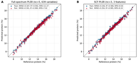
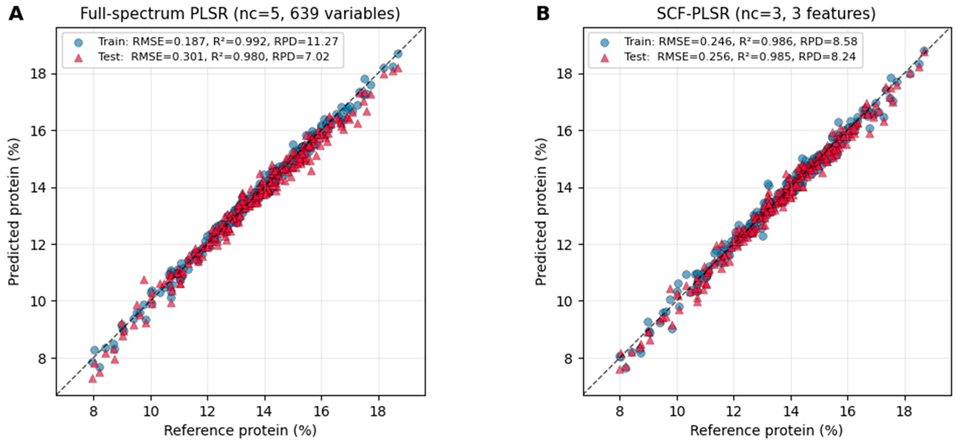
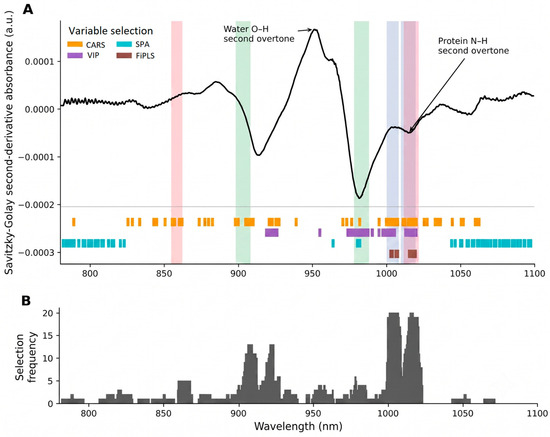
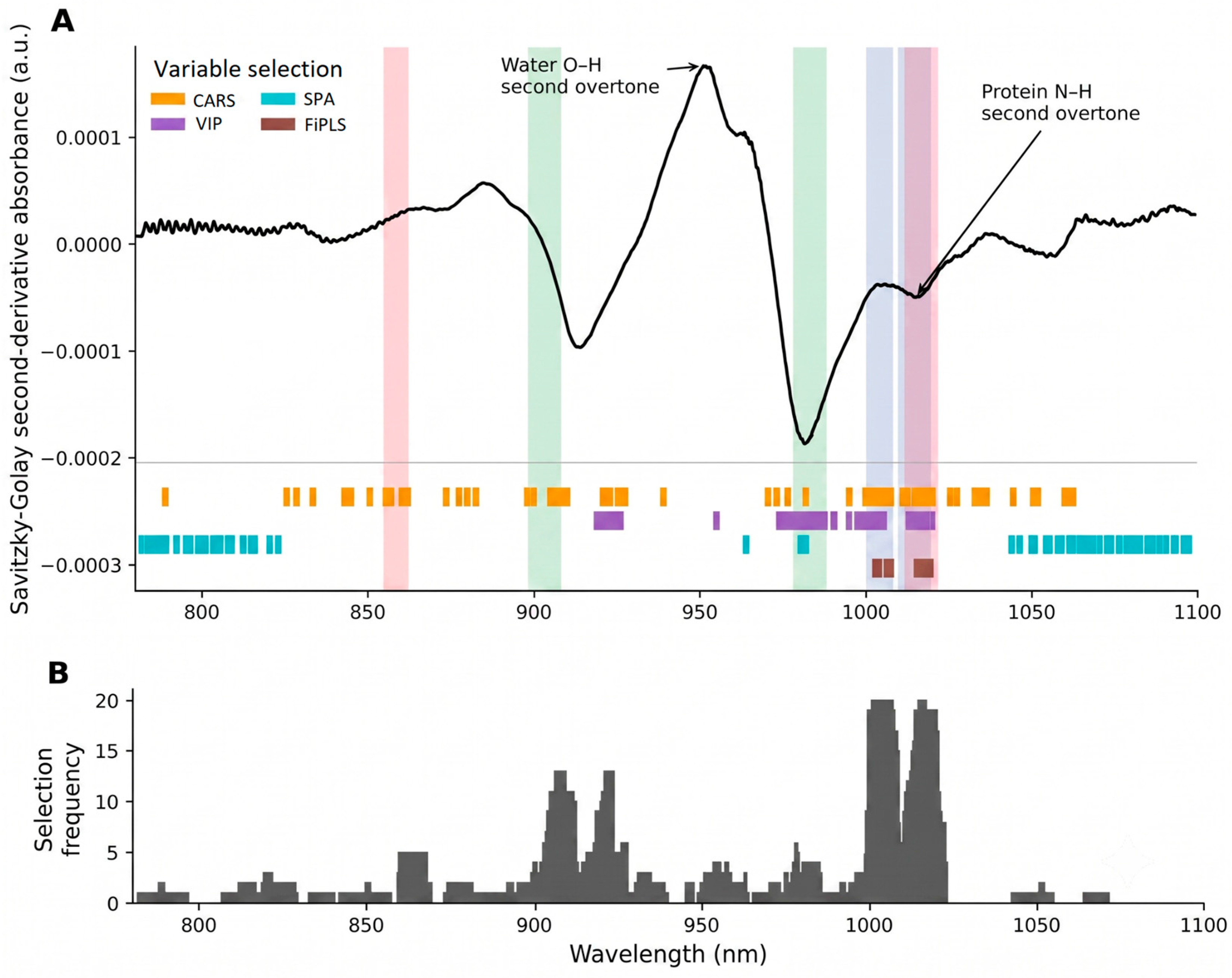
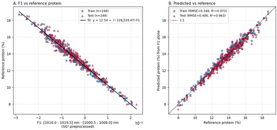
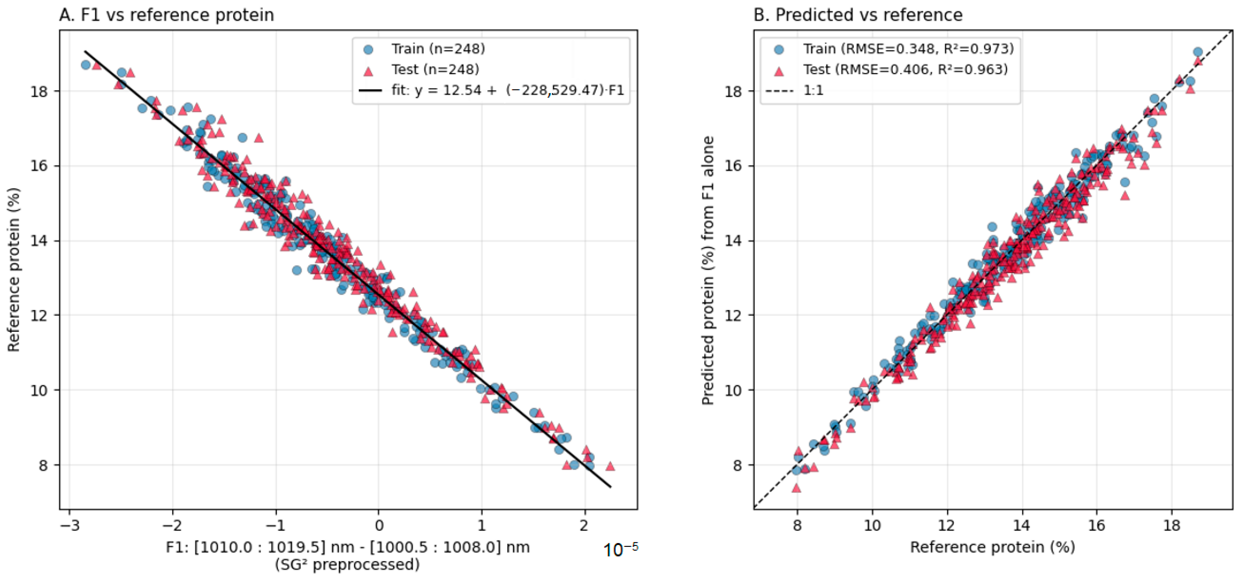
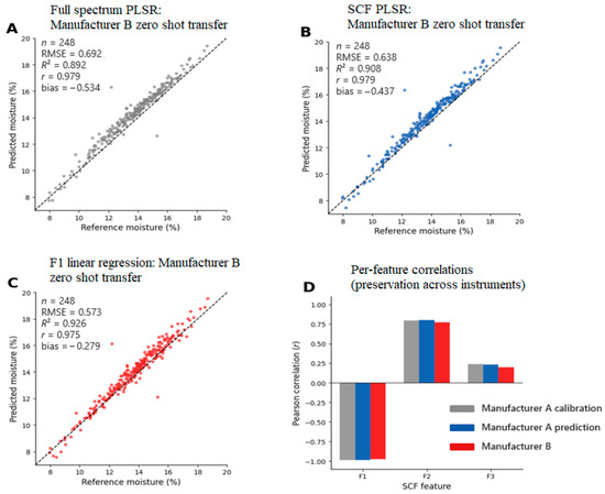
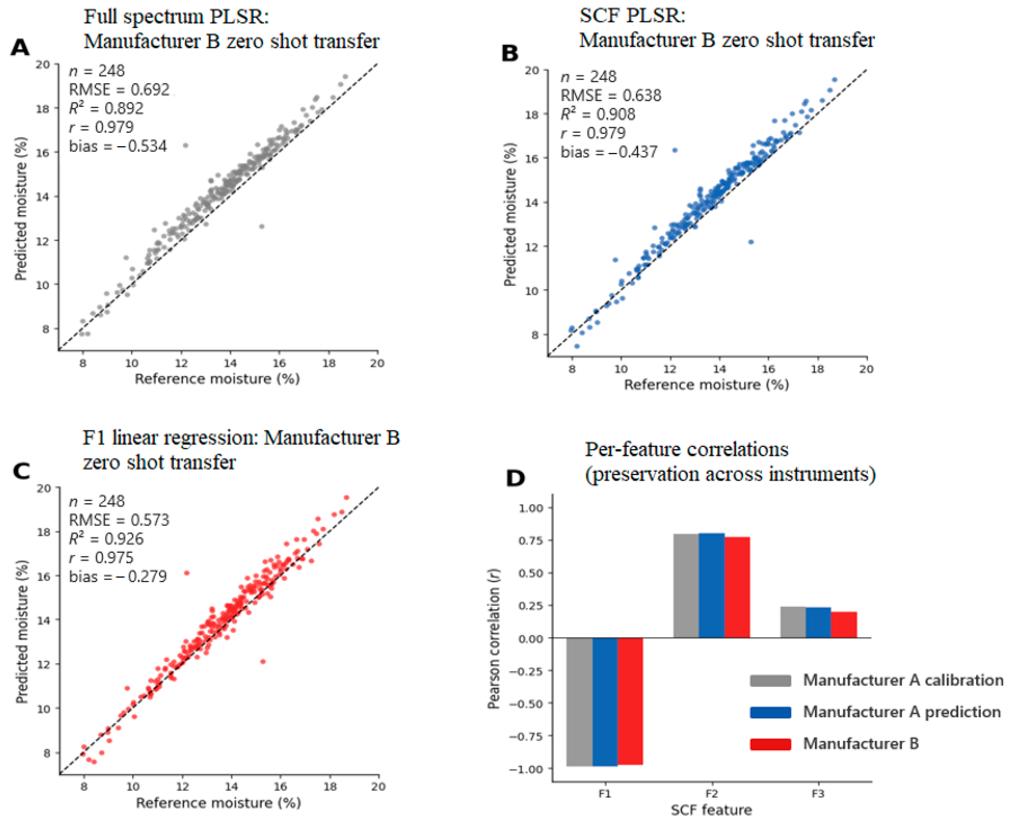
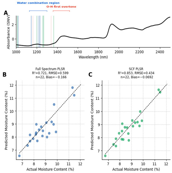
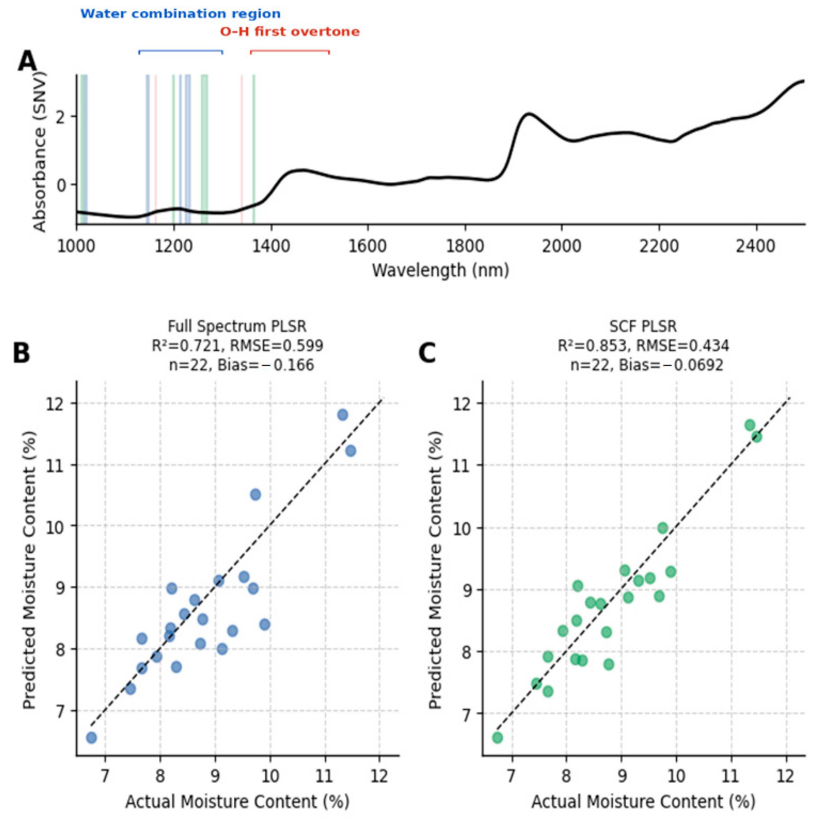
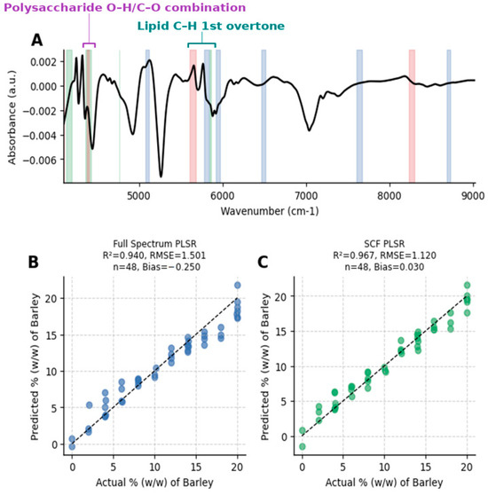
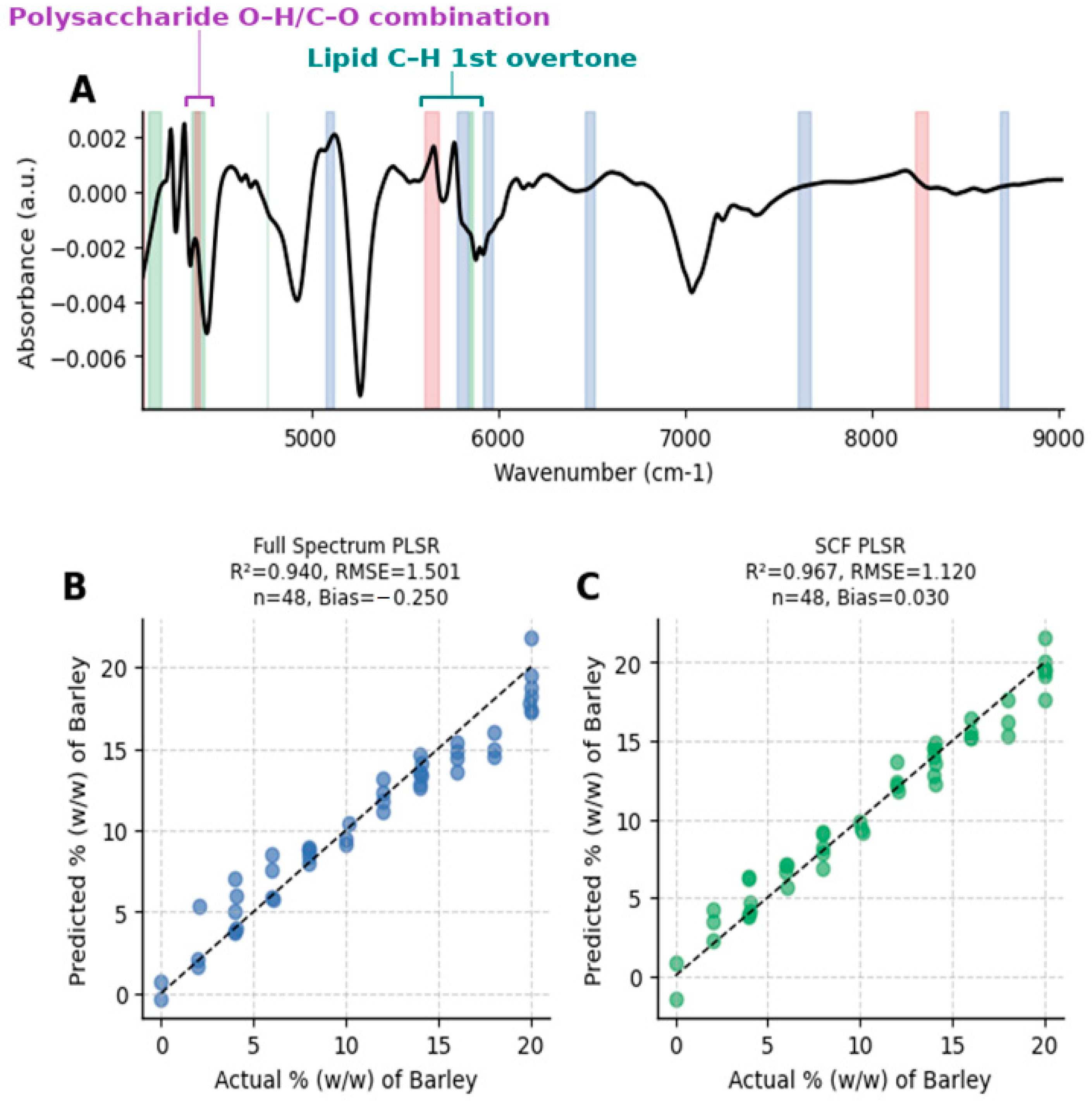
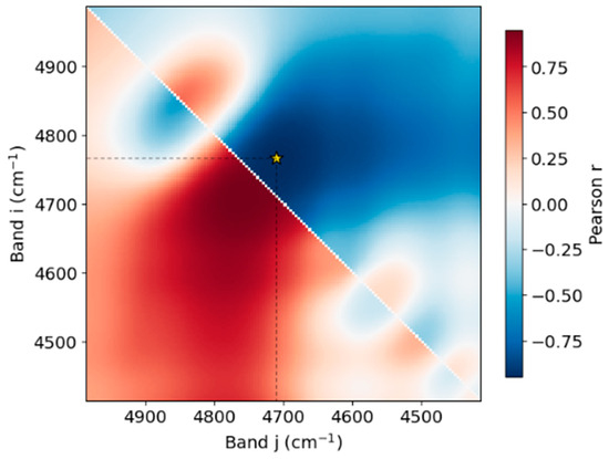
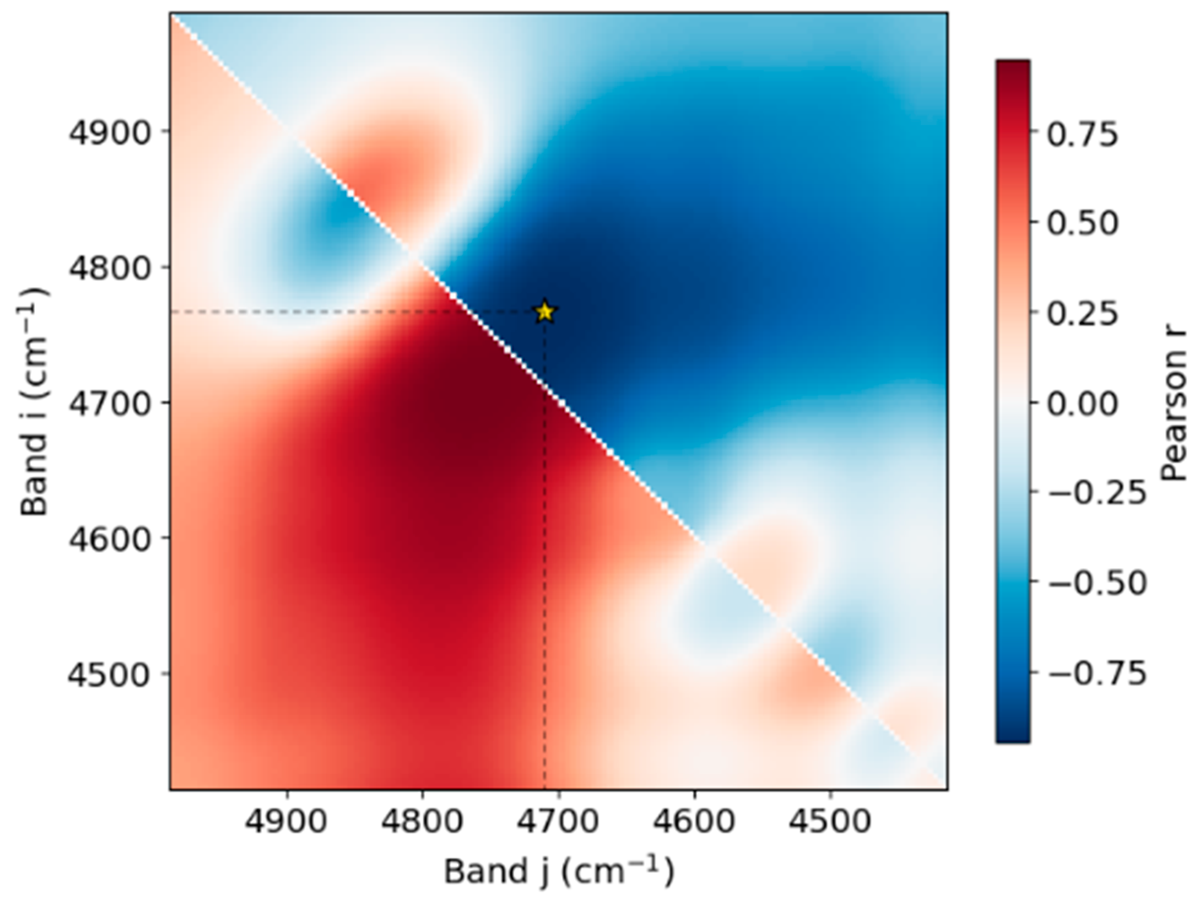
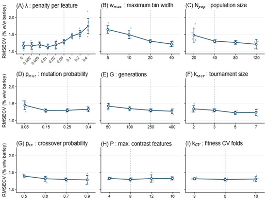
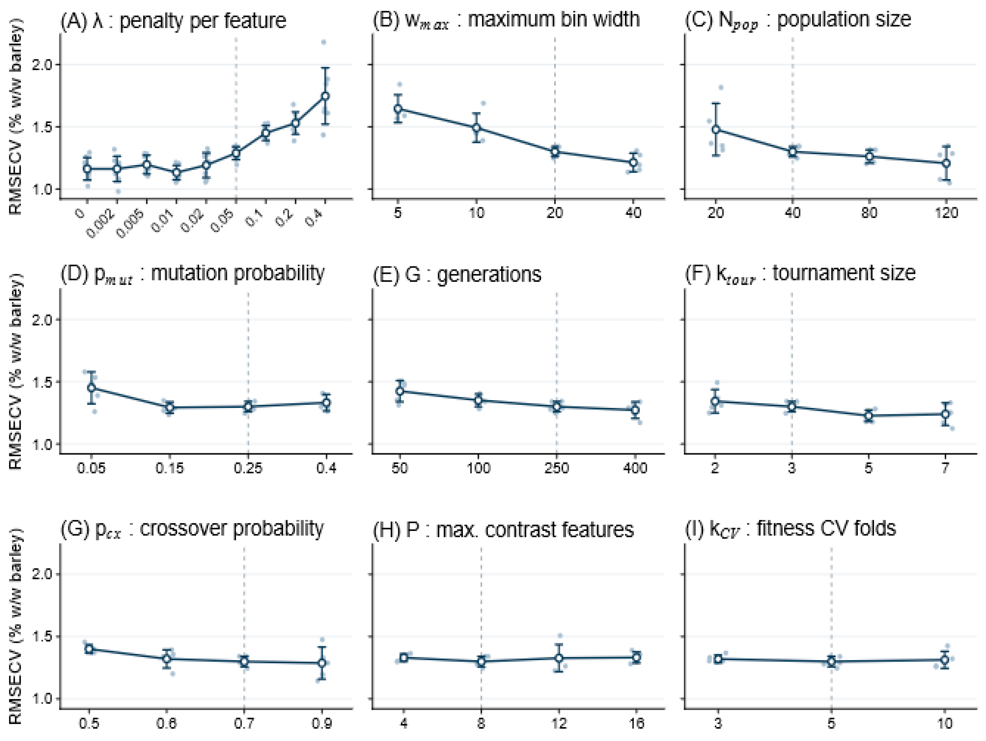
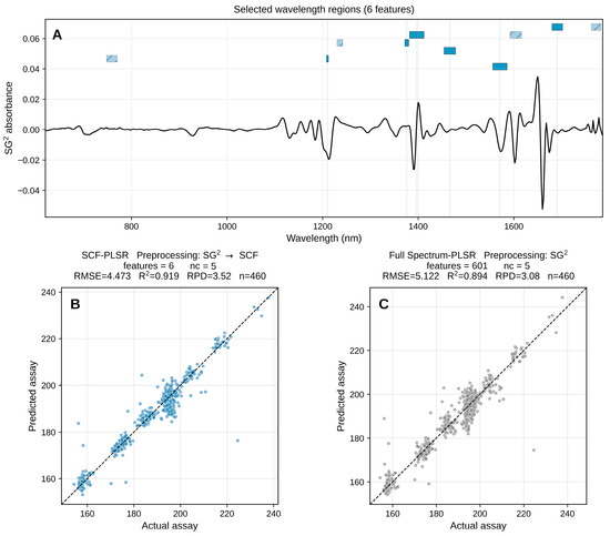
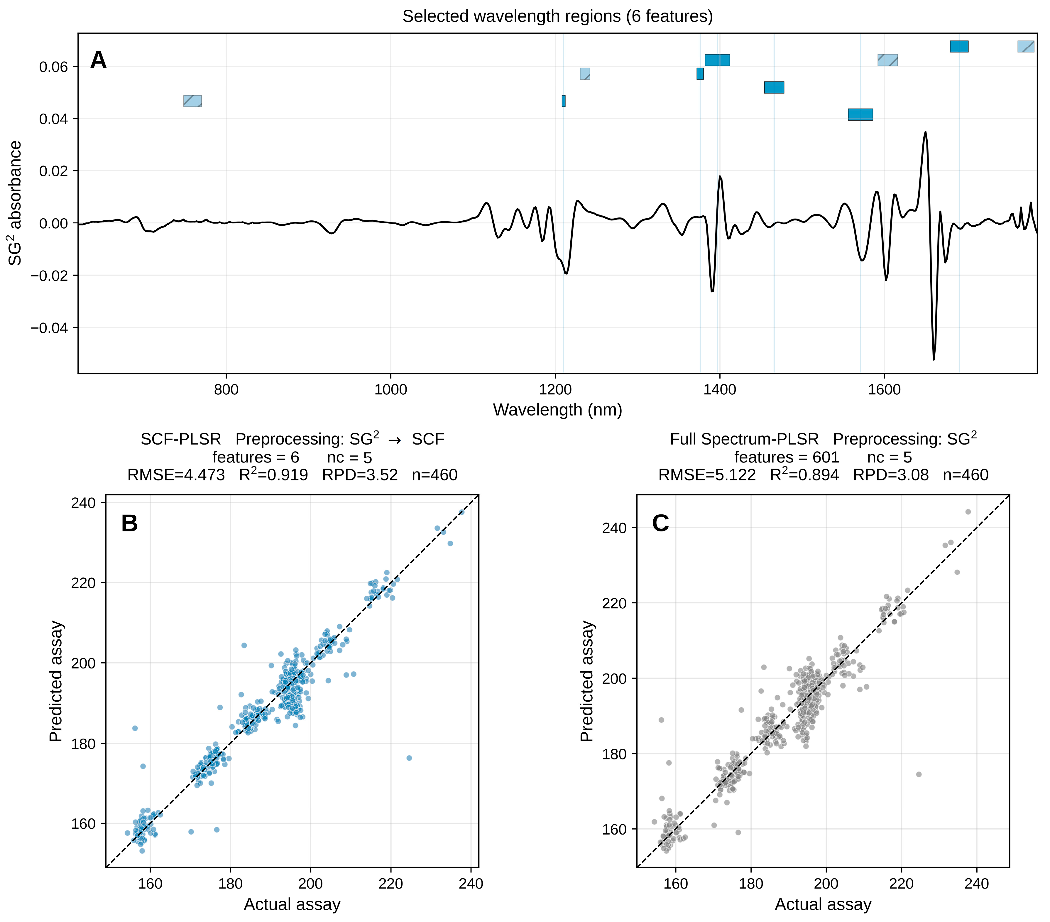

Disclaimer/Publisher’s Note: The statements, opinions and data contained in all publications are solely those of the individual author(s) and contributor(s) and not of MDPI and/or the editor(s). MDPI and/or the editor(s) disclaim responsibility for any injury to people or property resulting from any ideas, methods, instructions or products referred to in the content. |
© 2026 by the author. Licensee MDPI, Basel, Switzerland. This article is an open access article distributed under the terms and conditions of the Creative Commons Attribution (CC BY) license.