


Abstract
Real estate valuation in heterogeneous markets requires accurate and interpretable models. This paper evaluates Spatial Hedonic Residual Learning (SHRL), a two-stage framework combining Ridge hedonic regression with Random Forest residual learning. Using 1905 Dubai residential listings across 54 neighborhoods, evaluation includes six simulation scenarios, nested random-group and buffered geographic validation, ablation analysis, spatial diagnostics, and whole-model explanations. Random-group Mean Absolute Percentage Error (MAPE) is 15.68%, compared with 21.85% for Ridge, 19.31% for standalone Random Forest, and 14.92% for a spatial Gaussian-process comparator. Under geographic validation, SHRL MAPE increases to 28.17%, exceeding Ridge’s 25.41% and the spatial comparator’s 25.12%. Simulations likewise identify both gains and failure cases, while geographic residual clustering persists. Grouped explanations distinguish the structural contribution of the complete predictor from location-driven residual corrections. An independently refitted Singapore Housing & Development Board (HDB) transaction application achieves 5.60% chronological-test MAPE but higher unseen-town MAPE than Random Forest and boosting. Empirical prediction bands support descriptive listing price deviation screening, with substantial ambiguity rather than verified economic mispricing. The findings support task-dependent use of residual learning, with explicit limits on geographic transfer, economic interpretation, and uncertainty coverage.
1. Introduction
Real estate valuation is a central task in housing economics, investment analysis, mortgage lending, portfolio management, and market monitoring. Accurate price prediction provides buyers, sellers, lenders, investors, developers, and regulators with quantitative information about comparable properties. However, property prices are difficult to model because they depend on interacting sources of heterogeneity, including size, number of rooms, property condition, precise location, neighborhood characteristics, accessibility, views, and unobserved attributes. The interpretation of a prediction also depends on whether the observed outcome is an advertised price, a completed transaction, or an appraisal.
Hedonic pricing models provide a classical statistical approach to this problem. In the hedonic framework, a residential property is treated as a differentiated good whose price reflects its attributes [1,2]. The explicit specification helps analysts inspect fitted associations between those attributes and price. Nevertheless, a single global log-linear model may miss nonlinear relationships and interactions. Spatial patterns may also remain in its residuals, so nearby properties exhibit similar prediction errors. Moran’s I diagnoses spatial association, while spatial econometric models explicitly represent spatial lags or errors [3,4].
Machine learning models offer an alternative because they can learn nonlinearities and interactions without prespecifying a global parametric form. Random Forest (RF), gradient boosting, and XGBoost provide established ensemble learning approaches [5,6,7], including applications to real estate prediction [8]. Hybrid approaches can make a statistical baseline and its learned correction separately accessible for inspection. This principle is established in regression-kriging and methods combining flexible covariate effects with Gaussian process (GP) dependence [9,10,11]. The practical questions are when a particular residual learning implementation improves prediction, how its two layers contribute, and whether its gains persist when the prediction task changes.
This paper examines Spatial Hedonic Residual Learning (SHRL), a two-stage framework combining Ridge hedonic regression with RF residual correction. Let be the observed property price and its log-price. The fitted SHRL log-price prediction is
where is the fitted Ridge component, and is the RF correction learned from its training residuals. Within each candidate specification, both stages receive the same preprocessed predictors. Coordinates and neighborhood indicators permit location-dependent corrections, but the RF does not explicitly estimate a spatial covariance process. The layer decomposition describes the fitted algorithm rather than separately identified economic effects.
The main empirical application uses 1905 Dubai residential property listings across 54 neighborhoods and predicts advertised prices. Separate random-group and buffered geographic evaluations distinguish interpolation within the sampled market from prediction in held-out regions. An independent application refits the architecture to Singapore Housing & Development Board (HDB) resale transactions, assessing chronological prediction and transfer to unseen towns. The two markets provide different prediction settings; the Singapore application does not establish transaction values or asking-to-sale gaps for the Dubai listings.
The contributions of this paper are sixfold. First, it evaluates SHRL against Ridge, standalone RF, histogram gradient boosting, and a Ridge-plus-spatial GP residual comparator. Second, six contrasting simulation scenarios examine both gains and failure cases under linear, nonlinear, spatially dependent, and heterogeneous-noise mechanisms. Third, feature-block ablations and matched-layer comparisons distinguish the predictive contributions of available inputs and residual correction, complemented by coefficient stability and whole-model grouped explanations.
Fourth, the study separates training-based model selection from outer-held-out assessment through nested validation, following established principles for prediction evaluation [12,13]. Distinct geographic tasks reflect the importance of matching validation to the intended use [14]; paired resampling intervals provide explicitly conditional assessments of model differences. Fifth, it evaluates training-only price corrections and listing-price deviation screening using the Fair Value Deviation Index (FVDI) as a descriptive relative discrepancy, together with empirical prediction bands and tolerance ambiguity. These flags describe deviations from modeled listing prices rather than verified economic mispricing. Sixth, the Singapore transaction application tests the architecture in an independently refitted second-market setting, with temporal and whole-town evaluations.
The remainder of the paper is organized as follows. Section 2 reviews hedonic and spatial models, machine learning, contextual attributes, refurbishment information, and hybrid prediction. Section 3 presents SHRL, validation and uncertainty assessment, spatial diagnostics, simulations, ablations, and listing deviation screening. Section 4 reports the simulation, Dubai, and Singapore results, followed by discussion and limitations. Section 5 concludes and outlines future research directions. Appendix A details the simulation generator. Appendix B provides additional evaluation settings and results, including spatial diagnostics, coefficient stability, retransformation procedures, Singapore data and reproduction details, and further predictive comparisons.
2. Related Literature
2.1. Hedonic and Spatial Valuation Models
Hedonic pricing theory is one of the most widely used frameworks for estimating real estate values. It represents housing as a bundle of characteristics whose implicit prices are reflected in observed market prices [1]. Common predictors include size, rooms, age, quality, amenities, and location. Hedonic models are attractive because their coefficients describe associations under an explicit statistical specification [2]. Conventional additive or log-linear implementations may nevertheless miss nonlinear interactions, while coefficient interpretation and inference depend on specification and error assumptions. Smooth statistical alternatives, including generalized additive models, can relax linearity without requiring a fully unrestricted tree model [15].
Spatial dependence is particularly important in property markets. Similar properties may have different prices because of local amenities, waterfront access, transport links, or neighborhood conditions. When these factors are imperfectly observed, hedonic residuals may remain spatially autocorrelated. Moran’s I provides a classical diagnostic of spatial association [3], while spatial econometrics supplies models for spatial lags and spatial errors [4]. A residual diagnostic and an explicit spatial dependence model therefore serve different purposes. Giuffrida et al. [16] apply a Spatial Durbin Error Model to residential property prices in La Spezia, Italy, using a first-order queen-contiguity weight matrix. Their study illustrates an explicit treatment of spatial dependence and spillover relationships, which is distinct from the coordinate-based RF correction used in SHRL.
Spatial machine learning also extends beyond using coordinates as ordinary predictors. Georganos and Kalogirou [17] develop spatially weighted geographical Random Forests, whereas Chen et al. [18] incorporate geographic proximity alongside attribute similarity in spatially explicit nearest-neighbor prediction. These mechanisms differ from the single global RF correction used in SHRL. Supplying coordinates and neighborhood indicators permits location-dependent fitted relationships but does not itself specify a spatial covariance process.
2.2. Machine Learning and Explainable Real Estate Analytics
Machine learning models are increasingly used for real estate price prediction because they can learn nonlinear relationships and interactions. RF averages many decision trees [5], while gradient boosting and XGBoost provide alternative ensemble learning strategies [6,7]. For Dubai property data, Elnaeem Balila and Shabri [8] compare several machine learning algorithms. Such applications motivate comparison with flexible standalone predictors rather than relying exclusively on a linear benchmark.
Recent work also combines richer predictors, ensemble models, and explanation methods. Deng and Zhang [19] study a multilevel ensemble for Hong Kong apartment transactions, examining property characteristics, location, urban amenities, and accessibility. Rojas-Quiroz and Marmolejo-Duarte [20] combine spatial econometric modeling, XGBoost explanations, and clustering to examine housing-submarket patterns in Barcelona. These studies address both predictive flexibility and locational heterogeneity, but differences in outcomes, predictors, sample processing, and validation prevent direct comparison of their accuracy with the present Dubai results.
Despite their predictive flexibility, complex models may be difficult to interpret in valuation contexts. Shapley additive explanations (SHAP) provide an additive framework for attributing individual predictions to features under a specified explanation convention [21]. Explaining only a hybrid model’s correction, however, does not explain its complete prediction. The present study therefore examines the Ridge layer, RF correction, and combined SHRL predictor using the same grouped empirical Shapley game. The group definitions and training backgrounds make the explanation scope explicit; the resulting attributions describe fitted-model behavior rather than causal implicit prices.
2.3. Zonal, Socioeconomic, and Environmental Context
Location summarizes several distinct mechanisms that are better measured directly when reliable contextual data are available. Morano et al. [22] examine relationships between property prices, land use, and socioeconomic variables across municipalities in Apulia. Their municipal-scale analysis motivates attention to economic and territorial context, while also distinguishing area-level relationships from dwelling-level effects.
More recent applications illustrate complementary forms of contextual enrichment. Neves et al. [23] integrate contextual open data with tuned XGBoost and SHAP for Lisbon real estate prediction. Ko and Park [24] compare hedonic regression and RF for Seoul apartment prices while considering air pollution and other environmental and accessibility characteristics. These studies motivate measuring local conditions alongside structural attributes; they do not establish that any particular uncollected variable would necessarily improve prediction in Dubai.
Geographic representation and aggregation also matter. Kenyon et al. [25] use satellite image features and clustering to examine housing-submarket boundaries at different scales in Madrid. Jaroszewicz and Horynek [26] compare linear regression and RF for aggregated Warsaw asking price indicators without structural dwelling attributes. Administrative neighborhood labels, image-derived zones, and aggregated price units consequently describe different analytical objects. In the present data, coordinates and neighborhood labels may capture associations with several unmeasured contextual factors, but their predictive contribution cannot identify which factors they represent.
2.4. Refurbishment Costs and Property Condition
Refurbishment expenditure, physical condition, and policy exposure require separate treatment. Morano et al. [27] relate residential selling prices to ordinary municipal refurbishment cost benchmarks and other characteristics using an econometric model. Such benchmarks describe expected local costs rather than verified renovation expenditure for each dwelling. Mamre and Sommervoll [28] instead identify renovation status from listing text linked to Norwegian transactions and investigate renovation-related price differences using hedonic regression and RF. Their analysis also considers variation over time and the composition of transacted properties.
At a different scale, Wilhelmsson and Warsame [29] examine renovation subsidies and municipal housing market relationships in Sweden using panel and spatial econometric methods. Together, these studies show why cost benchmarks, observed condition, and subsidy exposure cannot be treated as interchangeable measures. The Dubai dataset contains none of these independently measured quantities: its supplied quality category is an amenity-count band. The literature therefore motivates a specific omitted-information limitation, rather than interpreting that category or its ablation as evidence about renovation costs or returns.
2.5. Hybrid Residual Learning Perspective
The proposed SHRL framework belongs to an established family of models combining a statistical component with a flexible correction. Regression kriging couples a regression trend with spatial prediction of residuals [9]. In a housing application, Cellmer and Kobylińska [30] incorporate information about kriged residual patterns into machine learning prediction of quoted Warsaw apartment prices. These precedents establish that learning from residual spatial structure is not, by itself, a new modeling principle.
Other hybrid methods estimate flexible covariate relationships alongside explicit dependence. Sigrist [10] combines boosting with Gaussian process and mixed-effects models. Gyger et al. [11] apply spatial machine learning with Gaussian process components and model explanations to German rental listings and a condominium-listing application. These models explicitly represent covariance in addition to nonlinear predictor effects. SHRL instead fits Ridge first and then an RF correction; the sequential Ridge-plus-GP comparator evaluated here is also distinct from joint GPBoost estimation.
Residual prediction studies further emphasize the importance of the observed target. Deppner et al. [31] use boosting to model deviations between commercial property appraisals and subsequent U.S. transaction prices. Those deviations are observable appraisal errors against sale outcomes. A discrepancy between a Dubai listing price and its model prediction has a different interpretation and cannot be assigned the same economic validation without corresponding transaction information.
Against this background, the present contribution is the evaluation of a sequential Ridge–RF architecture through controlled feature and layer comparisons, contrasting simulations, and distinct prediction tasks. Nested selection separates model choice from assessment [13], while dependence-aware validation should reflect whether the intended task is interpolation or transfer across locations or periods [14]. The Dubai random-group and buffered geographic evaluations, together with an independently refitted Singapore transaction application, examine these boundaries. They support assessment of when residual learning helps, rather than a claim that the architecture universally supersedes hedonic, spatial, or standalone machine learning models.
3. Methodology
3.1. Data and Variables
The dataset contains listed residential properties located in Dubai and distributed across 54 neighborhoods. The analyzed file is a processed CSV available through Kaggle [32,33]. Each observation corresponds to one property listing, rather than a verified unique dwelling. The target variable is the listed property price measured in AED. The main modeling response is the log-price,
where is the observed listed price of property i. The logarithmic transformation is used because the original price distribution is highly right-skewed.
The available predictors include structural variables, spatial variables, a source quality category, and amenity indicators. Structural variables are property size in square feet, number of bedrooms, and number of bathrooms. Spatial variables are latitude, longitude, and neighborhood. Amenity indicators include features such as balcony, pool access, gym access, covered parking, concierge service, security, water view, landmark view, and related listing attributes. Furnishing status is represented separately by the binary unfurnished indicator. In the supplied data, the four quality labels correspond exactly to the count of 27 amenity indicators, excluding unfurnished; the labels are Low for 0–5, Medium for 6–12, High for 13–19, and Ultra for at least 20 amenities. Thus, this variable summarizes amenity availability rather than independently measured finishing quality, renovation condition, or refurbishment expenditure.
Categorical variables are one-hot-encoded, with categories absent from a training partition represented by an all-zero block at prediction time. Numerical predictors are standardized using training-set means and standard deviations. Encoding and scaling are fitted separately within the relevant training partitions during model selection and final fitting. The variable price per square foot is used only for descriptive analysis and is excluded from all prediction models because it is directly derived from price and size and would introduce target leakage. The listing identifier is also excluded from the predictors.
The supplied CSV contains no missing values, and all 1905 records are retained in the main analysis without imputation or deletion based on price extremes. The associated project documents upstream scraping and cleaning procedures [34], although the complete raw-to-processed pipeline could not be independently verified. Repeated attribute profiles and shared coordinates are not treated as proof of duplicate dwellings; their grouping and sensitivity assessment are described in the validation procedure. Listing and collection dates are unavailable, and the original collection portal is undisclosed, preventing temporal validation or contemporaneous transaction price comparison for this sample.
Table 1 summarizes the dataset. Neighborhood sizes range from 1 to 302 listings; 34 neighborhoods contain fewer than 20 observations, including 4 singletons. Table 2 reports the complete distribution. These counts describe coverage of the supplied sample rather than its representativeness of Dubai’s housing stock.
Table 1.
Overview of the Dubai real estate dataset.
Table 2.
Distribution of the 1905 listings across all 54 source neighborhood labels. Entries are ordered by decreasing count, with alphabetical ties, reading down the left panel and then the right. Percentages use the full sample and are rounded to two decimal places.
3.2. Baseline Hedonic Models
The baseline hedonic model is
where represents the preprocessed hedonic predictors and is an error term. The predictor vector contains the structural, location, furnishing, and amenity-related variables included in the candidate specification, as defined in Section 3.1. Latitude and longitude enter this baseline linearly.
Ordinary Least Squares (OLS) estimates the coefficients by minimizing squared errors. Because one-hot encoded location and quality indicators may be correlated with other predictors, the main linear benchmark is Ridge regression. For a training partition , its coefficients are estimated as
where and . The intercept is not penalized; all predictor coefficients, including the one-hot neighborhood and quality coefficients when present, receive the Ridge penalty. Preprocessing follows Section 3.1; one-hot indicators retain their binary scale, and all training-observed categorical levels are included without an omitted reference category.
The penalty is selected from . Although coefficient estimation minimizes penalized squared log-price errors, penalty selection uses pooled inner-validation MAPE after exponentiating the log predictions. The Ridge benchmark independently selects its candidate feature specification using the nested procedure in Section 3.4; the selected model is then refitted on the complete outer-training partition.
The fitted hedonic prediction is denoted
The coefficients describe penalized fitted associations with log listing price under the selected specification; they are not interpreted as causal effects or independently identified economic implicit prices.
3.3. Spatial Hedonic Residual Learning
SHRL is estimated in two stages. First, a Ridge hedonic model is fitted on the training data. Second, a residual learning model is trained on the training residuals,
using the residual-feature vector , where denotes the relevant training partition. These are in-sample residuals from the Ridge model fitted on that partition; they are not cross-fitted residuals. The residual model estimates
where is learned by RF. Within each candidate feature specification, both stages use the same preprocessed predictors, so . Estimation is sequential, without joint optimization or backfitting; the fitted components are algorithmic prediction layers rather than separately identified economic effects.
The common predictor block comprises property size, bedrooms, bathrooms, latitude, longitude, neighborhood, and furnishing status. Four candidate specifications are evaluated: this common block alone; the common block plus quality; the common block plus the 27 individual amenity indicators; and the full set containing both quality and individual amenities. These contain 7, 8, 34, and 35 raw predictors, respectively, before one-hot encoding. Feature selection is performed within the outer-training data rather than by choosing the specification with the best outer-held-out score.
The final log-price prediction is given by Equation (1), where . Here, is the Ridge layer selected within the SHRL pipeline, which need not have the same feature specification or penalty as the independently selected Ridge benchmark. The predicted price is obtained by back-transformation,
This uncorrected inverse-log prediction is the primary reference; it is not automatically an estimate of conditional mean price or transaction value. Separate training-only retransformation adjustments are evaluated in Section 4.6, with formulas and selection details in Appendix B.
For each candidate feature specification, the Ridge penalty is first selected using pooled inner-validation MAPE, as described in Section 3.2. Conditional on that penalty, the residual RF is tuned using inner-validation predictions from the complete two-stage pipeline. Each forest uses 300 trees, bootstrap sampling, squared-error splitting, and no maximum-depth restriction. The minimum leaf size is selected from , and max_features is selected from . This is sequential tuning, not an exhaustive joint search over the Ridge and forest parameters. Algorithm 1 summarizes the nested evaluation procedure.
| Algorithm 1 Nested evaluation of Spatial Hedonic Residual Learning (SHRL) |
|
The term spatial refers here to the use of coordinates and neighborhood information as predictors. The RF can learn nonlinear location-dependent associations, but SHRL does not explicitly estimate a spatial covariance process, spatial lag, or spatial weight matrix. Random-group and buffered geographic evaluations therefore address distinct prediction tasks, as specified in the validation procedure.
The selected feature specification may differ across outer folds and validation designs. The block comparisons are specified in Section 3.7 and reported in Section 4.3; selection or exclusion of a block does not establish its economic importance or irrelevance.
3.4. Validation Protocol and Uncertainty Assessment
For the Dubai listing data, performance is evaluated using nested cross-validation with five outer folds and three inner folds under two distinct designs: random predictor group validation and buffered spatial validation. All preprocessing, feature and parameter selection, and model fitting are confined to the relevant training partitions; outer-held-out outcomes are reserved for evaluation. Separating model selection from evaluation avoids selecting a specification on the same predictions used to report its performance [13].
In random-group validation, records with identical values of all 35 available predictors are assigned to the same group, excluding the listing identifier, price, and price per square foot. Consecutive group identifiers are assigned in source-row order, giving 1878 groups. Shuffled GroupKFold uses seed 2026 for the outer partition and seed for the inner partition of outer fold . Folds are not stratified by price or neighborhood. These groups protect observable repeated predictor profiles but do not establish physical dwelling identity. Different records at the same coordinates may still occur in different random folds; this design therefore assesses interpolation within the sampled market.
Spatial validation keeps all records at each of the 728 distinct coordinate pairs together. For partition geometry, locations are represented in a local equirectangular coordinate system centered at latitude and longitude , with Earth radius m. Recursive coordinate cuts form approximately balanced geographic folds using listing counts as site weights. At each node assigned q folds, the coordinate axis with the largest range is selected, and a feasible cut between distinct coordinate values is chosen closest to the target listing share ; the two subsets are then partitioned recursively. Spatial inner folds are constructed anew using only the outer-training locations. Candidate training records less than 250 m from any held-out location are excluded from that fold’s training set, using haversine distances. Buffer exclusions are fold-specific rather than global record deletions. The 250 m separation is a prespecified assessment scale, not an estimated independence radius. These distinct designs reflect the dependence of validation on the intended prediction task [14].
Each listing receives one outer-held-out prediction per model and design. Primary scores are computed by pooling those predictions across the five outer folds, rather than averaging repeated-fold scores. Sensitivities retain the unrotated geographic partition with 0 m and 1000 m buffers and use a rotated partition with a 250 m buffer. Models are retuned within each design; favorable sensitivity results do not replace the primary 250 m evaluation. A separate random-group sensitivity removes additional exact non-ID record copies, retaining 1893 records, without asserting that repeated profiles necessarily represent duplicate dwellings.
Ridge, standalone RF, SHRL, histogram gradient boosting, and Ridge with a spatial Gaussian-process residual correction are compared using the same four candidate feature specifications and the same outer and inner partitions. Each family selects its own specification and parameters using pooled inner-validation MAPE. Full-feature references retain all 35 predictors while tuning parameters within training data. Ridge penalties and SHRL settings are specified in Section 3.2 and Section 3.3; standalone RF uses the same forest grid as the residual RF. Tied Ridge-penalty scores favor the smaller penalty. Other exact selection ties favor fewer raw predictors as well as lexicographic order of the parameter representation with keys sorted alphabetically. These finite, family-specific searches are not claims of exhaustive optimal tuning.
Histogram gradient boosting uses squared-error loss, 200 iterations, learning rate 0.05, L2 penalty 1, and disabled early stopping. Maximum leaf nodes are selected from and minimum leaf size from . The spatial GP comparator first selects its Ridge penalty, then selects an exponential residual covariance with m and noise-to-signal ratio . Kernel distances use the local metric coordinates. Training residuals are averaged at exact coordinate sites; for a site containing training records, the covariance diagonal receives . This is a sequential regression-kriging comparator with a fixed Ridge trend, not joint spatial generalized least squares [9].
An additional spline-Ridge reference augments the preprocessed linear predictor matrix with cubic marginal B-splines for size, latitude, and longitude and a tensor-product coordinate basis. Uniform knot counts and the Ridge penalty grid are tuned within training data; knots are fitted from training ranges, added basis columns are training-standardized, and spline extrapolation is constant. Its numerical failures are retained explicitly. An exploratory bounded-basis variant retains native basis scales and is evaluated separately from the standardized spline comparator, outside the primary uncertainty comparisons.
Performance is evaluated using Mean Absolute Error (MAE), Root Mean Squared Error (RMSE), Mean Absolute Percentage Error (MAPE), Median Absolute Percentage Error, RMSE, and on the log scale, and the proportions of predictions within 10% and 20% of the observed listed price. MAPE is the primary relative prediction error metric and the tuning criterion:
Its denominator gives relative rather than currency error, but underestimation errors are bounded by 100%, whereas overestimation errors are unbounded. Complementary losses and held-out errors by observed price segment and neighborhood are therefore reported rather than interpreting MAPE as sufficient evidence of valuation accuracy.
Model differences are assessed using paired conditional resampling of saved outer-held-out predictions. The primary resampling units are the 85 occupied 2 km square cells anchored at the fixed local coordinate origin. In each of 19,999 bootstrap draws, 85 cells are sampled with replacement, retaining every listing in each sampled cell with its multiplicity. The same draws are applied to all compared models and designs. Metrics are recomputed with the draw-specific listing count; in particular, each RMSE is recalculated before taking the model difference. Negative SHRL-minus-comparator error differences favor SHRL. The primary bootstrap seed is 20261014.
We report 95% conditional percentile intervals using linear percentile interpolation. For the eight primary MAPE contrasts (SHRL versus four competitors under two primary validation designs), an additional approximate conditional Bonferroni adjustment uses percentile tail probabilities . Other metric and sensitivity intervals are descriptive. Alternative resampling units are 500 m and 1 km cells, 2 km cells shifted by 1 km in both directions, exact coordinate sites, and neighborhood labels. Their seeds are , where denotes the primary definition and denotes these alternatives in the stated order.
These intervals condition on the fitted predictions and depend on the suitability of the resampling units and their exchangeability/dependence assumptions. They do not include full model-refitting uncertainty, eliminate shared-training dependence, or establish unconditional coverage. Fold-wise Friedman and Wilcoxon tests are therefore not used as primary evidence of model superiority. Separate complete nested random-group runs with seeds 2027 and 2028 assess split and model-randomness sensitivity on the same sample; their ranges are descriptive rather than confidence intervals.
The Dubai analysis uses Python 3.12.14, NumPy 2.3.5, pandas 2.2.3, SciPy 1.17.0, scikit-learn 1.8.0, and Matplotlib 3.10.8. Ridge uses the Cholesky solver. Stochastic inner fits use seed , and outer refits use , where s is the run seed, is the outer fold, and is the inner fold. Unspecified estimator parameters retain the defaults of the stated software version. The independently refitted HDB application uses its own dated sample, feature block, and validation design, as specified in Section 4.10 and Appendix B. Prediction-layer comparisons, coefficient stability, and whole-model explanation methods are described in Section 4.8, with supporting details in that appendix.
3.5. Spatial Residual Diagnostic Methods
To evaluate residual spatial dependence, Moran’s I is computed on outer-held-out log-residuals, . These diagnostic residuals are distinct from the in-sample residuals used to train the correction model. Let be a spatial proximity weight. Moran’s I is
Positive values indicate that nearby observations tend to have similar residuals [3]. Here, n denotes the number of units on the diagnostic support, rather than necessarily the number of listings.
Diagnostics are computed both for all 1905 listings and for the 728 distinct coordinate sites. Site residuals are arithmetic means of listing log-residuals at each exact coordinate pair, with equal weighting across sites. This separates listing-weighted dependence from patterns that are less influenced by the number of co-located records. Coordinate sites are not verified buildings or independent dwelling units.
The primary graph uses the eight nearest other units, based on haversine distances with Earth radius m. Self-links are explicitly excluded. All neighbors tied at the eighth-neighbor boundary within 0.001 m are included, so the actual degree may exceed eight. Binary neighbor relations are symmetrized by union and then row-standardized; row normalization need not preserve matrix symmetry. Sensitivities use and distance bands of 500 m, 1 km, and 2 km. Isolated units in distance band graphs retain zero rows, with the general normalization in Equation (10). Nearest-neighbor graphs can contain long edges in sparse areas and are not fixed-radius neighborhoods.
Permutation diagnostics use random relabelings of residuals over the fixed graph, seed 2026, and common permutations across matched model comparisons. The primary upper-tail value is
giving a minimum positive value of 0.0001. A lower-tail value reverses the inequality, and the additional two-sided diagnostic is . These are nominal fixed-graph diagnostic values: exchangeability of fitted held-out residuals is not established. Neither a small value nor a reduction in Moran’s I constitutes a test that one model has significantly less residual dependence than another, and failure to reject does not establish independence.
Distance correlograms and common-scale aggregated residual maps complement the global index. The correlogram uses unordered pairs of distinct sites in distance bands , , , , , (5000, 10,000], (10,000, 20,000], (20,000, 40,000], and above 40,000 m. It averages globally centered residual cross-products divided by the site-level population variance; these summaries are not Pearson correlations and need not lie between and 1. Pair counts are reported to expose sparse distance bands.
For the primary spatial holdout, within-fold mean centering, individual-fold diagnostics, and permutations restricted within folds assess sensitivity to fold-level patterns. Random-validation site means may combine predictions from different fitted outer-fold models, so these fold-specific site procedures are not applied to the random design. The diagnostics describe remaining spatial structure; they do not establish that the training buffer removes dependence.
3.6. Simulation Design
To evaluate the methodological behavior of SHRL independently of one real dataset, a simulation study is conducted using six contrasting data-generating mechanisms. Each scenario generates 30 independent datasets of observations. Log-price follows
where denotes spatial location, is a known affine hedonic component, is the scenario-specific nonlinear component, is a latent spatial or site effect, and is observation noise. Prices are obtained as . The square has an illustrative side length of 20 km; the generators are methodological stress tests rather than calibrated representations of Dubai.
The common observed predictors are log size, bedrooms, bathrooms, coordinates, seven binary listing attributes, and a four-level quality category. The synthetic quality category is generated directly, rather than constructed from amenity counts as in the empirical dataset. Every model receives the same 12 numerical predictors and one categorical block, without feature-set selection or access to latent site/cluster labels or truth components. Exact covariate distributions, coefficients, spatial-field normalization, scenario equations, and seed rules are specified in Appendix A.
Table 3 summarizes the six scenarios. They include a genuinely linear case, a smooth additive field, correlated spatial noise, structural–location interactions, shared site shocks, and regime changes with heterogeneous noise. These mechanisms are intended to expose both favorable and unfavorable conditions for residual learning. Several properties vary jointly between scenarios, so their differences do not identify the effect of a single mechanism.
Table 3.
Simulation scenarios. Noise scales refer to the log-price scale; latent effects are separate from observation noise.
Each dataset is evaluated under random-row interpolation and buffered geographic-region transfer, using three outer folds and two inner folds for each task. Spatial partitions use the recursive coordinate-cut procedure on the synthetic Euclidean domain, preserve entire exact sites, and exclude candidate training locations within 0.0125 units (250 m) of validation locations at both nesting levels. Random validation intentionally allows shared sites in N5. The buffer is much shorter than the 3.6 km dependence length in N3 and does not imply spatial independence.
The models compared are Hedonic Ridge, standalone RF, SHRL-RF, histogram gradient boosting, and the Ridge-plus-spatial GP residual comparator. Preprocessing and tuning use training data only, with pooled inner-validation MAPE as the selection criterion. Ridge penalties are selected from . SHRL and SpatialGP first select the Ridge penalty and then tune their residual stages. Standalone and residual forests use matched 80-tree budgets, minimum leaf sizes , and all/square-root feature sampling. Boosting uses 150 iterations, learning rate 0.05, L2 penalty 1, minimum leaf size 15, and maximum leaf nodes , with early stopping disabled. The GP uses exponential-kernel lengths domain units (2 and 6 km) and noise-to-signal ratios . The remaining conventions follow the corresponding empirical implementations. In N1 and N2, a prespecified sensitivity refits RF and SHRL with 160 trees while retaining the 80-tree-selected configurations and seeds, without retuning.
For each dataset, model, and task, performance is computed from all 700 pooled outer-held-out predictions. MAPE, log RMSE, and currency-scale RMSE are primary summaries, complemented by Median Absolute Percentage Error, MAE, log-scale , and signed log error. Known deterministic and realized signals provide separate diagnostic targets; they are not fitted competitors or generally optimal price predictors. No simulated outcome or prediction is clipped, and no extreme-price record is removed.
Models are paired within each independently generated dataset. We define the dataset-level difference for comparator m, so negative values favor SHRL. We report its mean, between-dataset standard deviation , Monte Carlo standard error , and pointwise 95% Monte Carlo interval
These intervals quantify simulation uncertainty under the specified generator and fitting procedure, not uncertainty for the empirical Dubai sample or simultaneous evidence of superiority across scenarios. Outer folds are pooled within each dataset and are not treated as independent replications. Thirty datasets may leave substantial Monte Carlo uncertainty for tail-sensitive currency losses.
3.7. Ablation Design
A block-wise ablation analysis is used to assess the contribution of different feature groups. The four candidate specifications described in Section 3.3 are evaluated separately with fixed predictor sets for Ridge, standalone RF, and SHRL. These comparisons assess the contribution of the amenity count quality summary both without individual amenity indicators and conditional on their inclusion.
Additional location ablations use the specification containing structural variables, coordinates, neighborhood, furnishing status, and quality, without individual amenity indicators. Coordinates, neighborhood, and both location blocks are removed in turn from both SHRL stages. Structural variables, furnishing status, and quality are retained throughout; the specification without location inputs is therefore not a structural-only model. A separate residual-stage ablation retains the fitted Ridge baseline and removes coordinates and neighborhood only from the RF correction, with its forest settings reselected within the training data.
The contribution of residual learning is assessed through matched Ridge–SHRL comparisons using the same predictors and Ridge penalty. All ablations use the random-group and 250 m buffered spatial validation designs, with preprocessing and parameter selection confined to the corresponding training partitions. The additional location and residual-stage ablations are diagnostic comparisons and are not added to the primary feature selection pool. Because model settings may change when a block is removed, the resulting error differences are conditional predictive contrasts rather than causal effects or an additive decomposition of predictive gains. The corresponding empirical results are reported in Section 4.3.
3.8. Listing Price Deviation Screening
The FVDI measures the relative difference between an observed listing price and its outer-held-out SHRL prediction:
A positive value indicates that the listed price is above the prediction, while a negative value indicates that it is below the prediction. The denominator is the predicted price, unlike MAPE, which uses the observed price. These deviations do not establish economic overpricing, underpricing, or fair transaction value.
For the point-based screening rule, a tolerance threshold gives
The reference threshold is . Sensitivity analyses also use , , and . These are illustrative prediction deviation thresholds rather than economically validated decision cutoffs. Being within tolerance does not establish that a property is fairly priced.
The primary uncertainty-aware screening rule uses empirical prediction bands on the log-price scale. Within each outer-training partition, three task-matched inner cross-fits provide absolute log-prediction residuals, conditional on that partition’s previously selected feature specification and model settings. Preprocessing and model fitting exclude the corresponding inner-validation rows, although those rows contributed to the earlier configuration selection. For random-group validation, a calibration score is the maximum absolute residual within an identical-predictor group; for spatial validation, it is the maximum within an exact coordinate site. Listing-level scores are examined separately as a sensitivity.
For m score units and nominal coverage c, the band half-width for outer fold k is the ascending score at rank , with if that rank exceeds m. The primary nominal level is , with examined as a sensitivity. For a held-out listing in fold k, the band is
A listing is flagged as above the prediction band if , below the prediction band if , and otherwise receives no directional flag. These are empirical reference bands evaluated on outer-held-out listings. Pooling residuals from different fitted models and conditioning on prior configuration selection preclude claiming an exact split-conformal or CV+ coverage guarantee.
A separate tolerance-support diagnostic uses the signed log discrepancy . At , the interval is compared with . Directional support requires the entire interval to lie above or below this tolerance range; within-tolerance support requires the entire interval to lie inside it. All remaining cases are classified as ambiguous. This symmetric multiplicative tolerance has price ratio limits , which differ from the point rule’s . The discrepancy interval is not a confidence interval for an unobserved fair value.
As an auxiliary check, three reserved-calibration choices per outer fold are evaluated separately. Random validation reserves 20% of whole predictor groups; spatial validation reserves one of three coordinate regions and excludes proper-training sites within 250 m of that region. Model selection and fitting use only the remaining proper-training data, and reserved residuals determine the band width. A marginal whole-group coverage interpretation requires exchangeable calibration and new-group scores, an assumption not established by geographic separation alone. The results from the three choices are reported separately.
Coverage, relative band width, subgroup behavior, and flag stability are assessed alongside point-threshold sensitivity. The results of these analyses are reported in Section 4.9. No rule is interpreted as validated mispricing detection, and an unflagged or ambiguous listing is not classified as fairly priced.
4. Experimental Results and Discussion
4.1. Descriptive and Statistical Evidence
Table 4 reports the main descriptive statistics. The original price variable is strongly right-skewed, with skewness equal to 6.14. After the log transformation, skewness decreases to 0.71. Figure 1 and Figure 2 show the same transformation visually. All 1905 listings are retained; price per square foot is descriptive only and is excluded from prediction models.
Table 4.
Descriptive statistics of the main numerical variables. Price is measured in AED. Standard deviations use the sample convention; skewness is the standardized third central moment.
Figure 1.
Distribution of observed property prices. The distribution is strongly right-skewed because of high-value listings.
Figure 2.
Distribution of log-transformed property prices. The transformation substantially reduces skewness.
Table 5 reports descriptive effect magnitudes using all 54 neighborhoods and all four quality categories. Neighborhood membership accounts for 45.44% of the sample variation in log-price in a separate one-factor decomposition, compared with 2.32% for quality. These overlapping shares are not additive, do not control for other predictors, and do not establish causal premiums or held-out predictive importance. Quality is an amenity count category rather than an independent condition assessment. The sample contains 728 distinct coordinate sites, and 34 neighborhoods have fewer than 20 listings. Figure 3 displays the geographic coverage, sample density, and held-out regions.
Table 5.
One-factor descriptive associations with log listing price, retaining all 1905 listings. Degrees of freedom describe the between/within sums-of-squares partition; no inferential p-values are reported.
Figure 3.
Observed coordinate sites, listing density, and the five held-out geographic regions. Coordinates are displayed in local kilometers; named anchors are sample coordinate medians rather than neighborhood boundaries. Blank areas contain no sampled listings.
4.2. Simulation Results
The six scenarios in Section 3.6 and Appendix A examine both favorable and unfavorable conditions for residual learning. Table 6 and Figure 4 report mean MAPE across 30 independently generated datasets per scenario. Uncertainty in paired differences is shown in Figure 5; the replication unit is the dataset, not the validation fold.
Table 6.
Mean simulation MAPE (%) across 30 independent datasets per scenario and task. Each dataset contributes one pooled outer-held-out score per model. Pointwise Monte Carlo intervals are shown in the figures.
Figure 4.
Mean simulation MAPE and pointwise 95% Monte Carlo intervals for each fixed generator and evaluation task. These intervals quantify simulation precision, not uncertainty about performance in Dubai.
Figure 5.
Paired simulation MAPE differences—SHRL minus each comparator, with pointwise 95% Monte Carlo intervals across 30 datasets. Negative values favor SHRL. These are separate generator/task comparisons without a simultaneous multiplicity guarantee.
Under the correctly specified linear scenario N1, residual learning adds a small error: SHRL minus Ridge is +0.16 MAPE points in random validation, with a 95% Monte Carlo interval of [0.12, 0.19], and +0.17 [0.11, 0.24] geographically. In the smooth additive scenario N2, SHRL improves over Ridge by 15.40 points under random interpolation but deteriorates by 6.37 [5.12, 7.61] points under geographic transfer. The spatial GP comparator has lower mean MAPE than SHRL in both N2 tasks. Learning a smooth residual within the observed region therefore does not ensure geographic transfer.
The other scenarios further qualify the architecture’s usefulness. Under correlated spatial variation in N3, the geographic SHRL–Ridge difference is −1.49 [−3.26, 0.28] points. In the interaction scenario N4, geographic boosting and RF achieve 25.28% and 26.08% MAPE, respectively, compared with 29.61% for SHRL. In N5, the gain from sharing observed sites in random validation disappears for unseen sites: the geographic SHRL–Ridge difference is +0.58 [−0.16, 1.32] points. In N6, SHRL improves on Ridge, while its geographic difference from boosting is unresolved at +0.01 [−1.47, 1.50] points. An interval containing zero does not establish equivalence.
The forest-size sensitivity from 80 to 160 trees produces small MAPE changes in N1 and N2 and does not remove the N2 geographic failure. Rankings also depend on the loss: in N4 geographic validation, SHRL has higher MAPE than boosting but lower AED RMSE by approximately AED 1.26 million. This scenario includes extreme synthetic prices, so the currency loss comparison has substantial Monte Carlo uncertainty. The simulations support conditional predictive value under the specified generators and finite tuning grids, rather than universal superiority or an economically calibrated Dubai mechanism.
4.3. Ablation Analysis of Feature Blocks
Table 7 and Figure 6 distinguish amenity/quality comparisons from controlled removal of location inputs. The common seven-predictor block contains size, bedrooms, bathrooms, coordinates, neighborhood, and furnishing status. Adding quality gives 8 predictors; adding individual amenities gives 34; including both gives the full 35-predictor specification. The location removal comparisons use the eight-predictor specification as their common anchor.
Table 7.
Fixed-feature ablations: pooled held-out MAPE (%). Parameters are selected within training data for each specification. The last three rows remove inputs from the common-plus-quality anchor, retaining structural variables, furnishing status, and quality.
Figure 6.
Matched Ridge and SHRL errors for fixed feature specifications. The dashed line separates the four candidate feature specifications from the three location removal diagnostics. The no location input does not mean structural variables alone.
For random-group interpolation, SHRL’s common block has MAPE 15.68%, compared with 17.02% for the full specification. Under geographic validation, the corresponding values are 27.72% and 27.65%. Thus, the random benefit of omitting individual amenities does not establish that those attributes are noisy or economically irrelevant, or that one parsimonious specification is universally optimal. All five primary random SHRL fits select the common block; the spatial fits select it in three folds, individual amenities in one fold, and the full specification in one fold.
Removing coordinates from the quality-containing anchor raises SHRL MAPE from 15.87% to 20.28% randomly and from 28.06% to 32.96% spatially. Removing neighborhood gives 15.79% and 30.84%, respectively. Removing both location blocks gives 35.47% and 42.17%. A separate residual-stage ablation, retaining the Ridge baseline, changes MAPE by +5.94 points randomly and −2.48 points spatially when both location inputs are removed from the forest alone. Location information is predictively useful, but its contribution depends on the task and layer; the ablations do not identify causal neighborhood effects.
4.4. Predictive Performance Under Interpolation and Geographic Transfer
Table 8 reports pooled outer-held-out performance for the five independently inner-selected pipelines with uncorrected back-transformation. Each listing contributes one prediction per model and validation design.
Table 8.
Primary pooled held-out performance for 1905 Dubai listings per design. MAPE and Median APE are percentages; MAE and RMSE are in million AED. Log-scale quantities use natural logarithms.
Under random-group validation, SHRL achieves 15.68% MAPE, compared with 21.85% for Ridge, 19.31% for RF, and 17.52% for boosting. Spatial GP has the lowest point MAPE at 14.92%, but the largest AED RMSE at 2.787 million, compared with 1.529 million for SHRL and 1.123 million for boosting. Lower average percentage error therefore coexists with larger currency errors; no single metric establishes uniform superiority.
Geographic transfer is more difficult. SHRL MAPE increases to 28.17%, while Ridge and spatial GP achieve 25.41% and 25.12%, respectively. SHRL remains below RF and boosting in point MAPE, but the architecture does not outperform the linear baseline in this primary transfer task. Figure 7 shows both tasks without averaging them into one score.
Figure 7.
Primary pooled held-out MAPE under random-group interpolation and 250 m buffered geographic transfer. Each model independently selects its configuration using the corresponding inner-training procedure.
Figure 8 retains all held-out observations and predictions for all five models on logarithmic price axes. The complete AED-axis display is provided in Appendix B. Observed prices span AED 0.22–35 million, whereas the largest random-validation predictions reach approximately AED 79.43 million for SHRL and AED 129.64 million for spatial GP. These predictions remain in all error calculations. SHRL’s highest observed-price quintile has MAPE 20.43% randomly and 36.46% geographically. These strata are post-outcome diagnostics; the errors do not by themselves identify missing-variable causes.
Figure 8.
All 1905 outer-held-out listings per model and task, with common logarithmic price axes spanning every observed and predicted value. The diagonal marks equality. No extreme prediction is removed.
The fixed full-feature comparison in Table A5 retains all 35 eligible raw predictors for every model family, while tuning parameters within training data. With these common inputs, random-group MAPE is 19.98% for RF and 17.02% for SHRL, compared with 21.96% for Ridge and 16.39% for spatial GP. Under geographic validation, the corresponding values are 36.49%, 27.65%, 25.39%, and 25.36%. These additional references do not replace the independently feature-selected primary pipelines.
Table A6 reports MAPE and currency RMSE for all five models across all five observed-price quintiles under both primary designs. These descriptive post-outcome strata expose variation in errors across the price distribution without using observed-price groups for model fitting or selection.
Spatial sensitivity changes the ranking: spatial GP has the lowest point MAPE for the 0 m and primary 250 m buffers, while SHRL has the lowest for the 1000 m buffer and the rotated partition. SHRL’s respective MAPE values are 25.73%, 28.17%, 25.39%, and 26.48%. These are different declared validation designs, not interchangeable estimates from which the most favorable score is selected. Extra nested random seeds give SHRL MAPE 15.54% and 15.23%, compared with the primary 15.68%; these are descriptive reruns on the same sample.
The standardized tensor-spline comparator suffered extreme extrapolation and failed positive-price conversion in some held-out cases. A separately evaluated bounded-basis variant yielded random/geographic MAPE of 21.43%/26.10% but remains exploratory because it was introduced after diagnosing those failures. Neither its results nor the failed configurations replace a primary competitor.
4.5. Conditional Uncertainty in Model Differences
Table 9 reports paired MAPE differences using 19,999 resamples of the 85 occupied 2 km cells, retaining all listings in each sampled cell. The intervals condition on the saved predictions and prior model selection. They do not quantify the full uncertainty of retraining the algorithms or eliminate all cross-fold and spatial dependence. The adjusted columns apply the declared eight-comparison Bonferroni percentile rule.
Table 9.
SHRL minus comparator MAPE differences in percentage points. Negative differences favor SHRL. Both interval columns are conditional percentile summaries, with approximate multiplicity adjustment in the final column.
Random-group differences favor SHRL over Ridge, RF, and boosting under both displayed interval conventions. The random SHRL–spatial GP gap of +0.76 points has a pointwise interval [−0.09, 1.43], leaving its direction unresolved. Under primary geographic validation, the adjusted intervals favor Ridge and spatial GP over SHRL, while the SHRL–boosting-adjusted interval includes zero. The corresponding secondary spatial GP–Ridge difference is −0.30 points with pointwise interval [−2.33, 1.33].
The sign patterns of pointwise MAPE intervals persist across the six declared resampling-unit choices for SHRL versus Ridge, RF, and boosting randomly, and versus Ridge and spatial GP geographically. This sensitivity does not establish population coverage. Independent-fold Friedman and Wilcoxon tests are not used as evidence for model superiority.
4.6. Retransformation and Price Calibration
The uncorrected exponential predictions remain the primary reference. Additional training-only cross-fit analyses compare six correction methods: identity, a MAPE-oriented global multiplier, global smearing, an AED least-squares multiplier, log intercept/slope adjustment, and smearing by predicted-price bins. Separate selectors choose among these methods using inner MAPE or inner AED RMSE. These procedures condition on the previously selected base configuration; correction coefficients and choices never use outer-held-out outcomes. Appendix B gives the formulas and selection details. Table 10 summarizes the SHRL retransformation sensitivity.
Table 10.
SHRL retransformation sensitivity. MAPE is in percent and RMSE in million AED. Fixed methods and training-selected procedures are separately defined analyses; none is selected using this outer-results table.
The MAPE-selected correction reduces random SHRL MAPE from 15.68% to 15.34% but raises geographic MAPE from 28.17% to 32.15%. Its conditional random MAPE-change interval is [−0.63, 0.01] points; all ten adjusted primary correction effect intervals across the five families and two tasks include zero. Global smearing brings the random aggregate predicted/observed price ratio closer to one, from 0.982 to 1.009, while worsening MAPE to 16.49%. Aggregate agreement and individual prediction accuracy are distinct. Smearing does not convert a listing price model into a verified transaction value model, and the favorable fixed spatial multiplier cannot replace the less favorable training-selected procedure after observing test results.
4.7. Spatial Residual Diagnostics Results
Table 11 reports the primary diagnostics for held-out log-residuals at both listing and equal-site support. The listing graph includes distinct listings at identical coordinates: 39.58% of its directed relations have zero distance. Aggregating to the 728 coordinate-site means changes both the weighting target and the graph.
Table 11.
Moran’s I and nominal upper-tail permutation p-values from 9999 permutations on the declared graphs. Listing and site supports are distinct diagnostics, not repeated estimates of one parameter.
Random SHRL residuals have listing , compared with 0.3561 for Ridge and 0.1805 for RF; SHRL’s site mean value is −0.0145. Geographic SHRL residuals remain strongly structured, with listing/site values of 0.5705/0.4071, exceeding Ridge’s 0.4926/0.3570 and spatial GP’s 0.4876/0.3218. The random spatial GP values are negative on both supports, with nominal two-sided ; its large upper-tail p-values do not establish absence of spatial association.
The geographic SHRL diagnostic remains positive after fold centering and within-fold permutation, and each individual held-out region has positive site-level I. Site-residual standardized similarity is 0.2858 for pairs up to 250 m apart and approximately 0.154–0.156 from 250 m to 2 km. A 250 m training buffer therefore cannot be interpreted as an estimated independence radius. Figure 9 and the additional diagnostics in Appendix B expose the remaining structure. Permutation values are nominal fixed-graph diagnostics, not tests of between-model superiority.
Figure 9.
Cell-median held-out log-residuals for Ridge, RF, and SHRL under both tasks, using a common color scale spanning all five primary models. Positive residuals refer to listings above predictions. Dots mark cells with fewer than 20 listings; blank cells have no records. The maps summarize observed errors, not a fitted geographic correction surface.
4.8. Prediction Layers and Whole-Model Explainability
To isolate the residual layer, SHRL is compared with its own matched Ridge component rather than the independently tuned Ridge benchmark. Adding the forest changes MAPE from 21.84% to 15.68% randomly but from 25.51% to 28.17% geographically. Table 12 shows the paired conditional changes. The forest’s correction aligns strongly with held-out Ridge errors under random interpolation and much less strongly under geographic transfer; a non-zero correction is not necessarily an improvement.
Table 12.
Combined SHRL minus its matched Ridge layer. Negative changes favor the correction. Pointwise intervals reuse the 19,999 occupied-cell draws and condition on the fitted models.
The Ridge layer retains inspectable penalized associations. Across the five primary random fits, median log contrasts are +0.3959 per 1000 sqft, +0.1762 per bedroom, and +0.0332 per bathroom; geographic medians are +0.3865, +0.1879, and +0.0324. The six core numeric coefficient signs persist across all 15 random seed-fold fits. These are descriptive stability summaries of overlapping fits, not coefficient confidence intervals or causal premiums. All-level categorical encoding has no omitted reference category; the reported category profiles are centered within each training fit. Appendix B gives coefficient ranges and local-response curves.
Whole-model explanations use a four-player empirical grouped Shapley game: structural profile; location profile; quality/amenity profile; and furnishing status. For each task, 30 label-free sampled held-out cases per fold are explained by their own fold model using two 32-record outer-training backgrounds. All 16 coalitions are enumerated; global summaries weight each explained case by its fold population divided by 30. Identical replacement inputs are used for Ridge, the forest correction, and their sum, verifying that their signed local attributions add exactly. This finite marginal replacement game preserves relationships within blocks but can break dependence between blocks; it does not estimate causal effects or population conditional expectations. Table 13 and Figure 10 display the grouped attributions for both validation tasks.
Table 13.
Weighted mean absolute grouped Shapley values in log-price units, using the primary 32-record background and 150 explained held-out cases per task. Absolute attribution magnitudes are not additive importance shares.
Figure 10.
Grouped empirical Shapley magnitudes for both layers and their combined prediction. Bars use the primary training background; markers show the second background. Structural profiles dominate the combined predictor, while location dominates the RF correction. These are fitted-model explanations relative to sampled reference records.
For combined random predictions, the structural and location magnitudes are 0.3710 and 0.3088 log units, respectively; within the correction they are 0.0472 and 0.0905. The same reversal appears geographically. Thus a residual-only ranking does not describe the full predictor. The amenity block has zero attribution in primary random fits because those selected models omit it, not because amenities have no economic value. The top-two ranking persists under the second background and a six-player structural-grouping sensitivity, but individual attribution levels and signs depend on the reference. Retaining Ridge improves the visibility of the model’s layers without identifying economic effects in the full nonlinear predictor.
4.9. Listing Price Deviation Analysis
Using Equation (14), the point deviation sensitivity analysis in Table 14 and Figure 11 reports above-, within-, and below-tolerance listings. At 15%, 729 listings (38.27%) are outside the point tolerance under random validation, compared with 1205 (63.25%) geographically. These are prediction discrepancy counts, not verified overpricing or underpricing. Empirical prediction-band coverage and directional flags are summarized in Table 15.
Table 14.
Point-based FVDI threshold sensitivity for uncorrected held-out SHRL predictions. Counts use the point-based relative deviation rule, with ratio limits . Within tolerance does not mean fairly priced.
Figure 11.
Shares above, within, and below each illustrative point tolerance. The expanding within-tolerance group is a mathematical consequence of widening the cutoff and does not validate an economic decision threshold.
Table 15.
Empirical SHRL prediction band assessment. Coverage and flag rates are percentages. Width is the full band span divided by its point prediction, not a symmetric ± percentage. Whole-group coverage requires every listing in a predictor group or coordinate site to be covered.
At nominal 90%, the empirical bands cover 91.76% of random held-out listings and 91.39% of geographic held-out listings, while giving directional flags for 157 (8.24%) and 164 (8.61%) listings, respectively. Their median full widths are 75.45% and 141.55% of the point prediction. Fewer flags therefore reflect broader uncertainty ranges rather than improved point prediction accuracy. Whole-site geographic coverage is 89.56%, differing from listing-weighted coverage. Figure 12 shows the geographic distribution of held-out prediction-band coverage.
Figure 12.
Geographic distribution of held-out 90% SHRL band coverage on fixed 2 km cells. Counts and sparse-cell markings are retained. These are post-prediction coverage summaries, not maps of economic mispricing or calibrated local guarantees.
With the separate 15% symmetric multiplicative tolerance support rule, 51 random and 96 geographic listings have directional support, none has within-tolerance support, and 97.32%/94.96% remain ambiguous. This rule has a different lower ratio bound from the point-based FVDI rule. No directional flag, ambiguity, and within-point-tolerance status must not be relabeled as fair pricing.
The auxiliary reserved-calibration experiments show sensitivity to calibration choice: nominal-90% random listing coverage ranges from 88.92% to 90.39%, and geographic coverage from 90.92% to 96.12%. Across three complete random nested seeds, 94.54% of primary 90% band labels agree, but direction-specific pairwise Jaccard overlap is only 0.576–0.659. High overall agreement is partly driven by the many unflagged listings. The 90% band covers only 82.15%/75.59% of the highest observed-price quintile, versus 91.76%/91.39% overall.
Table 16 selects the ten largest neighborhoods by listing count, with alphabetical ties, independently of their errors or deviation signs. It reports medians and interquartile ranges of alongside empirical coverage. Appendix B reports mean, median, dispersion, and extrema for all 54 neighborhoods. For Jumeirah Beach Residence, geographic median D is 0.495 and band coverage is 56.03%, exposing substantial local variation despite the overall coverage figure. Sparse categories and unmeasured listing characteristics limit interpretation; these patterns do not identify their economic causes.
Table 16.
SHRL summaries for the ten largest neighborhoods by listing count. ; brackets contain the first and third quartiles, not confidence limits. Coverage refers to empirical nominal-90% bands.
4.10. Independent Application to Singapore Resale Transactions
An independent application uses the official Singapore HDB resale dataset supplied through data.gov.sg under the Singapore Open Data Licence [35,36]. The analyzed snapshot contains 242,634 records and 11 fields; the declared development window uses 80,306 transactions from 2022–2024, with 25,084 transactions in 2025 reserved for chronological testing. Repeated observable profiles are retained because no unit identifier establishes duplicate dwellings. Source characteristics, exclusions, and reproduction settings are documented in Appendix B.
All four models use log floor area, storey-interval midpoint, remaining lease, registration-month index, town, flat type, and flat model. The response is log resale price, with uncorrected exponential back-transformation. Training-only preprocessing and pooled inner MAPE determine settings. Chronological selection trains on 2022/validates on 2023 and trains on 2022–2023/validates on 2024; a separate five-fold whole-town outer evaluation with two inner town folds uses only the development window. The finite grids are reported in Appendix B. Without verified coordinates, this is a categorical location-aware refit of the architecture rather than a distance-buffered replication or transfer of Dubai-trained parameters. Table 17 and Figure 13 summarize the held-out results for both evaluation tasks.
Table 17.
Independent HDB application: pooled held-out errors. MAPE and median APE are percentages; MAE and RMSE are in SGD. The geographic task holds out whole categorical towns without a distance buffer.
Figure 13.
MAPE in the independent HDB application. The chronological test predicts 2025 from 2022–2024; unseen-town evaluation holds out complete towns within 2022–2024. SHRL is refitted on HDB features in each task.
The SHRL adaptation achieves 5.60% chronological MAPE, versus 7.04% for Ridge, 8.07% for RF, and 5.70% for boosting. Its difference from boosting is −0.093 points, with a town-cluster conditional interval [−0.302, 0.104]. Under unseen-town evaluation, SHRL MAPE is 12.13%, compared with 13.15% for Ridge, 10.52% for RF, and 11.03% for boosting. The SHRL–RF and SHRL–boosting differences are +1.604 [0.424, 2.668] and +1.095 [0.378, 1.743] points. These pointwise intervals use 2000 resamples of the 26 towns and condition on the fitted predictions, without establishing independence between towns or retraining uncertainty.
SHRL has the lowest unseen-town currency RMSE, RF the lowest MAPE and MAE, and boosting the lowest log RMSE. Doubling the forests to 160 trees with selected settings fixed leaves the MAPE ordering unchanged. In the chronological test, 96.17% of transactions share a town/block/street address with development records, so that task largely concerns known-address forecasting rather than unseen locations. The extension provides an observed-transaction application in another market; it does not validate economic screening labels or asking-to-sale gaps for the original Dubai listings.
4.11. Discussion
The results support a conditional role for sequential hedonic residual learning. First, the six simulation scenarios show that a learnable residual can improve interpolation, while residual fitting can add error to a correctly specified linear model or fail geographically. Stronger nonlinear and spatial comparators change the apparent ranking. The framework’s usefulness depends on the residual structure, available inputs, deployment task, and loss function.
Second, the Dubai ablations establish predictive value for location information but do not justify a universal amenity exclusion rule or a causal interpretation of neighborhood differences. Training-selected specifications differ across tasks. The paired layer analysis further shows that the RF correction improves random interpolation while worsening the primary geographic MAPE. Random validation and geographic transfer answer different questions, and their scores should not be combined into a single accuracy claim.
Third, an inspectable Ridge layer and whole-predictor explanations provide complementary information. Structural profiles have the largest attribution magnitudes in the combined predictor, whereas location dominates the RF correction. Coefficients remain penalized associations, and the Shapley game remains a background-dependent fitted model explanation. Neither the sequential architecture nor attribution additivity establishes economic identification.
Fourth, uncertainty-aware screening reveals the limited resolution of listing-deviation classifications. Wide bands reduce directional flags and leave most listings ambiguous at a 15% tolerance. Overall coverage conceals weaker expensive-listing and local performance, and coverage remains empirical rather than a verified conditional guarantee. FVDI discrepancies can motivate further investigation but cannot determine fair transaction values, profitable investments, or economic mispricing accuracy.
Finally, the HDB extension demonstrates that the architecture can be independently refitted to observed transactions in a second market, with favorable chronological prediction but weaker unseen-town MAPE than nonlinear baselines. The remaining boundaries of the data, evaluation, and interpretation are brought together in Section 4.12.
4.12. Limitations
The Dubai analysis uses a processed listing sample whose original collection portal, collection dates, and complete upstream cleaning history could not be verified. The absence of dates prevents temporal evaluation and alignment with contemporaneous Dubai transactions. Observable predictor groups and coordinate sites do not establish dwelling identity, so grouping cannot guarantee separation of every repeated physical property. Unequal neighborhood coverage and sparse local samples limit precise subgroup assessment, and the sample does not establish representativeness of Dubai’s housing stock. Floor level, building age, renovation condition, and developer reputation are unavailable; the supplied quality category summarizes amenity counts rather than independently assessed property condition.
The Dubai response is advertised listing price rather than completed transaction price. Neither predictive accuracy nor FVDI deviations validate economic overpricing, underpricing, or investment returns. The Singapore HDB extension supplies an independent transaction-target application but does not resolve the original Dubai asking-to-sale gap. It refits the architecture using different attributes and categorical towns without verified coordinates; it therefore does not establish direct transfer of Dubai-trained parameters or replication of the coordinate-based spatial specification.
Performance depends on the task, loss, and finite tuning grids. SHRL’s random-interpolation gains do not persist against Ridge and spatial GP in the primary geographic MAPE comparison. Sequential tuning and the tested partitions, buffers, and forest budgets do not establish optimality or robustness across markets and periods. The simulations use illustrative generators with jointly varying mechanisms and a fixed sample size; thirty replications leave limited precision for extreme-price currency losses.
The paired resampling intervals condition on fitted predictions and rely on the suitability of the chosen geographic units; they exclude full retraining uncertainty and do not remove all dependence. Moran permutation values remain nominal diagnostics. The primary prediction bands use cross-fitted residuals conditional on prior model selection, so their empirical coverage does not establish an exact conformal or subgroup guarantee. Wide bands, local undercoverage, and substantial tolerance ambiguity restrict screening resolution; independent economic labels are unavailable to assess mispricing precision or recall.
Finally, Ridge coefficients remain penalized associations, and grouped Shapley values depend on the reference background. Grouping does not preserve all dependence between feature blocks. Stable coefficients and additive attributions do not identify causal premiums, and omitted amenities cannot be assumed economically irrelevant.
5. Conclusions
This paper proposed Spatial Hedonic Residual Learning as a structured data analytics framework for housing price prediction. The method combines a hedonic regression layer with a nonlinear residual learning layer. The hedonic layer provides an inspectable statistical baseline, while the residual layer learns corrections whose predictive usefulness depends on the data structure and evaluation task. The six simulation scenarios demonstrate gains when residual patterns are learnable, a small penalty in the correctly specified linear case, and failures in some geographic transfer scenarios.
The empirical analysis used 1905 Dubai residential property listings across 54 neighborhoods. Under nested random-group validation, SHRL-RF achieved a pooled MAPE of 15.68%, compared with 21.85% for Ridge, 19.31% for standalone RF, and 17.52% for boosting. The spatial GP comparator had a lower point MAPE at 14.92%, although its paired conditional difference from SHRL was unresolved and its AED RMSE was larger. Under the primary 250 m buffered geographic evaluation, SHRL MAPE increased to 28.17%, exceeding Ridge’s 25.41% and spatial GP’s 25.12%. These results distinguish interpolation gains from geographic transfer performance and show why rankings must be assessed across complementary losses.
Spatial diagnostics showed lower random-validation residual association for SHRL than for Ridge and RF, but substantial clustering remained under geographic validation. Whole-model explanations also qualified the residual-layer interpretation; structural profiles had the largest attribution magnitudes in the combined predictor, whereas location profiles dominated the RF correction. The framework makes these layers accessible for inspection, but neither its coefficients nor its grouped Shapley values identify causal property premiums.
The independent Singapore HDB application extended the analysis to observed resale transactions. The refitted SHRL adaptation achieved 5.60% MAPE on the 2025 chronological test, with an unresolved small difference from boosting. Its unseen-town MAPE of 12.13% was lower than Ridge’s but higher than RF’s and boosting’s. This additional application supports the architecture’s use beyond the Dubai listing sample while retaining the distinction between known location prediction and transfer to new locations.
The FVDI provides a descriptive listing price deviation measure, complemented by empirical prediction bands. The bands expose substantial uncertainty, and most listings remain ambiguous under the separate 15% tolerance support rule. Above- or below-model flags therefore support further investigation rather than verified economic overpricing, underpricing, or fair transaction value.
The principal limitations are consolidated in Section 4.12. They include incomplete Dubai collection provenance and dates, unobserved property characteristics, uneven sample coverage, finite model searches, and conditional uncertainty assessments. The HDB transaction application does not validate asking-to-sale gaps for the original Dubai listings.
Future work should prioritize dated Dubai transactions, building-level attributes, further market and period evaluations, and independent assessment of prediction band coverage and screening decisions. Overall, combining hedonic regression, residual learning, spatial diagnostics, and whole-model explanations provides a structured approach to housing price prediction and listing review, with benefits that depend on the intended deployment task.
Author Contributions
Conceptualization, methodology, software, validation, formal analysis, investigation, resources, data curation, writing—original draft preparation, writing—review and editing, visualization, supervision, and project administration, J.E.M. and A.A. All authors have read and agreed to the published version of the manuscript.
Funding
This research received no external funding.
Data Availability Statement
The Dubai listing dataset was obtained from the publicly accessible Kaggle dataset propertiesData, available at https://www.kaggle.com/datasets/mahaaghaei/propertiesdata (accessed on 22 October 2026). The Singapore HDB resale transaction dataset is publicly available through data.gov.sg at https://data.gov.sg/datasets/d_8b84c4ee58e3cfc0ece0d773c8ca6abc/view (accessed on 22 October 2026) under the Singapore Open Data Licence. Dataset provenance, sample selection, preprocessing, and evaluation settings are documented in Section 3 and Appendix B.
Acknowledgments
The authors would like to thank the Year 2 undergraduate Data Science students at Saint Joseph University, Dubai, for their assistance in the preliminary exploration of the dataset and in producing descriptive statistical summaries used during the early stages of this study.
Conflicts of Interest
The authors declare no conflicts of interest.
Appendix A. Simulation Generator Specification
Each scenario generates 30 datasets of 700 observations on , with one domain unit equal to 20 km. Locations are independent uniform draws in N1, N2, and N6. In N3 and N4, locations are drawn from Gaussian clusters with centers
selection probabilities , and isotropic displacement SD 0.06. Out-of-domain draws are resampled around the same center. N5 uses 100 sites drawn by this mechanism, with seven observations per exact site and no jitter.
Generate and size . Room counts follow
where . Quality codes denote standard, good, premium, and luxury, with probabilities and corresponding log-price premiums .
Let and . The attributes are water view, pool, gym, parking, concierge, security, and unfurnished status. They are conditionally independent Bernoulli draws with probabilities
The common affine signal is
where . Since , the signal is affine in the supplied log-size predictor.
Define
The normalized field uses the mean and population SD on the fixed grid , independently of each simulated sample. Set , where 0.2475 is the uniform-domain regime area. The nonlinear components are
Latent effects are zero except in N3 and N5. In N3, is a zero-mean Gaussian vector with
where the diagonal term stabilizes Cholesky generation. In N5, , with 100 independent shocks shared within sites. Independent Gaussian observation noise has SD 0.16 in N1, N2, and N4; 0.10 in N3; and 0.12 in N5. In N6,
The mixing indicators and Gaussian innovations are mutually independent and independent of the covariates. Prices follow Equation (12) by exponentiation, without outcome clipping or deletion.
Input columns are ordered as log size, bedrooms, bathrooms, u, v, water view, pool, gym, parking, concierge, security, and unfurnished status, followed by all-level one-hot quality indicators. Standardization and category vocabularies are fitted within each training partition; unseen categories have all-zero indicator blocks. No latent variables, site/cluster identifiers, or true signals are supplied as additional predictors. Ridge uses Cholesky estimation with an unpenalized intercept. Forests use bootstrap sampling, squared-error splitting, unrestricted depth, minimum split size 2, and one thread. GP site averaging and diagonal noise adjustment follow the empirical comparator, using synthetic Euclidean distances.
For scenario and replication , NumPy uses
to supply separate location, covariate, and noise streams through default_rng. Let g = 9,092,026 + 100,000a + 1000r. Random outer splits use ; inner splits in outer fold use . For design (random) or (spatial), let : inner stochastic fits use , , and outer fits use . Compared forests share phase seeds; spatial partitions use deterministic coordinate cuts.
Ridge-penalty ties favor the smaller penalty; other exact score ties follow lexicographic sorted-key parameter representations. Software versions are reported in Section 3.4. Round-trip floating-point loading and consistent matrix layout support numerical reproduction; results need not be bitwise identical across platforms.
Appendix B. Additional Evaluation Details and Results
Appendix B.1. Full-Range Predictions and Spatial Diagnostics
Figure A1, Figure A2 and Figure A3 complement the main-text prediction and residual diagnostics. All 1905 listings and extreme predictions are retained.
Figure A1.
Full-range AED-axis predictions for all five primary models and both tasks. Common axes include every prediction, including extreme extrapolations. The main-text logarithmic display resolves the compressed central cloud.
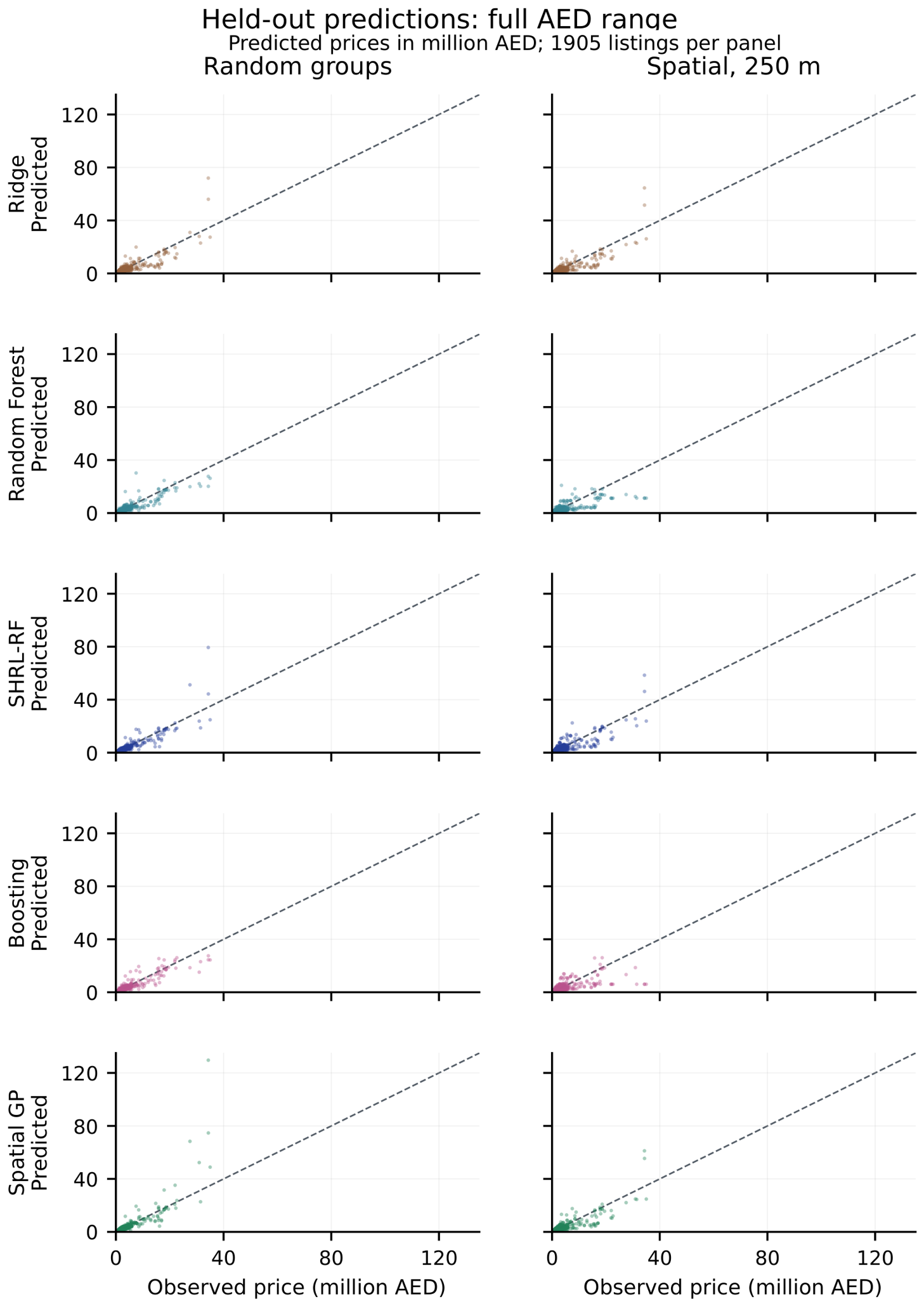
Figure A2.
Boosting and spatial GP cell-median held-out log-residuals on the common scale used for the main-text Ridge/RF/SHRL maps. Dots mark cells with fewer than 20 listings; blank cells contain no observations. These summaries do not establish local model superiority.
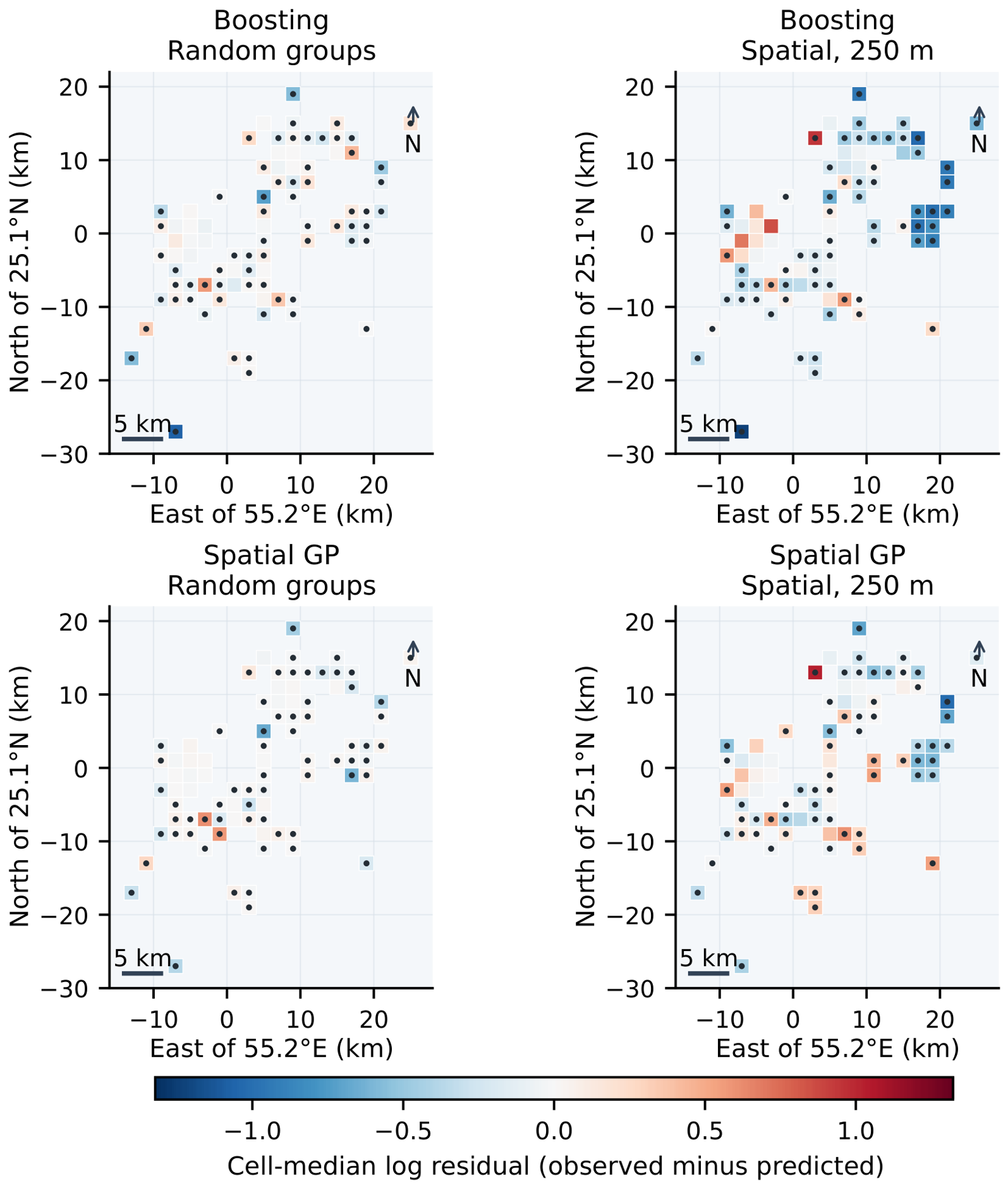
Figure A3.
Distance-binned standardized cross-products of equal-site log-residuals, not Pearson correlations. All 264,628 unordered site pairs are included; the terminal bin contains only 74 pairs from 54 sites and does not establish a long-distance process. The pale shaded areas in the lower panels mark the km terminal bin.
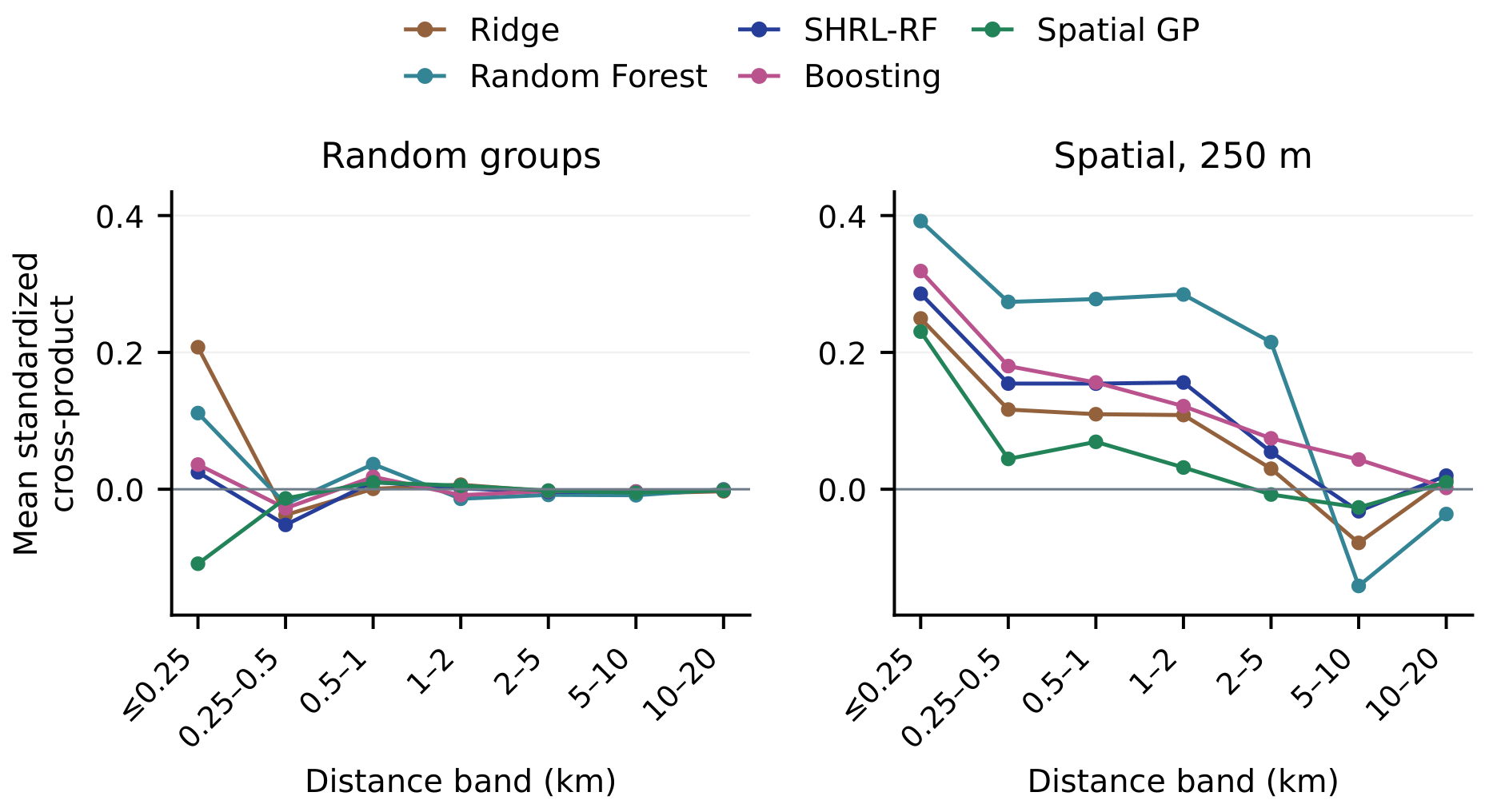
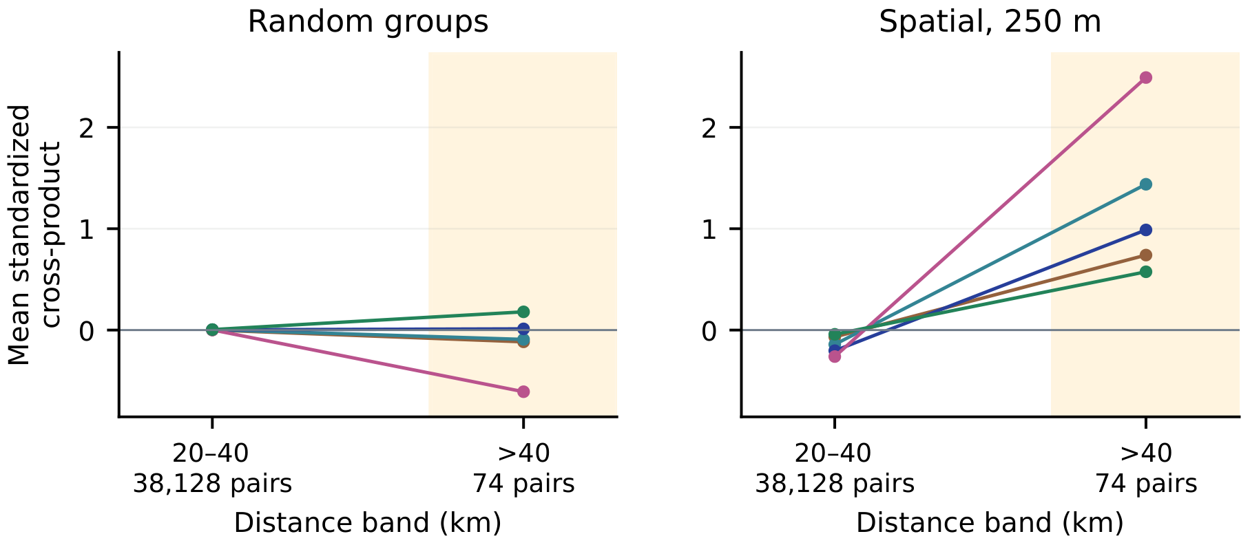
Appendix B.2. Coefficient Stability and Local Responses
Table A1 reports fixed-unit SHRL Ridge-layer contrasts. Raw-unit slopes divide standardized coefficients by their training scales; coordinate increments use the fixed display latitude. Ranges describe five overlapping fitted models per task, not confidence intervals or causal premiums.
First-order accumulated local effects [37] use each model’s outer-training distribution, up to ten unique quantile intervals for continuous features, and observed integer boundaries for room counts. Within-bin upper-minus-lower predictions are averaged, accumulated at bin midpoints, and centered by training-bin frequencies. All tail intervals are retained. The five curves per layer and task are fitted responses, not confidence bands; finite perturbations can still violate cross-feature dependence.
Table A1.
SHRL Ridge-layer log contrasts: median [minimum, maximum] across five outer-fold fits per task. Every reported coefficient is present in all five fits.
Figure A4.
Structural accumulated local effects for the Ridge layer, RF correction, and combined SHRL prediction. Curves use training profiles and retain all size intervals, including the full observed range in the bin construction. They describe model responses rather than causal interventions.
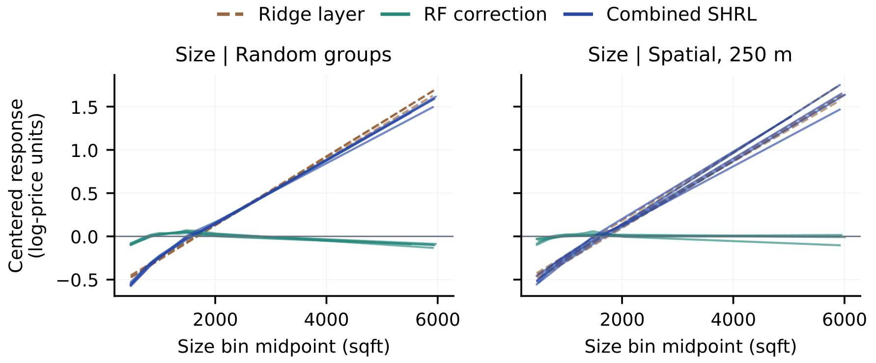
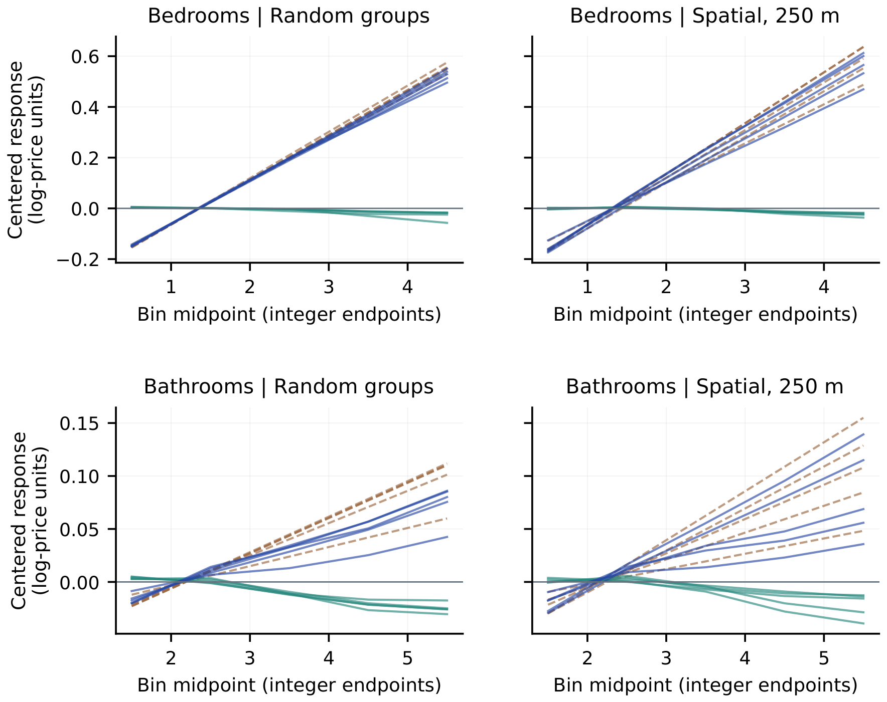
Appendix B.3. Retransformation Definitions
Let be a training cross-fitted log prediction, , and . Table A2 defines the six candidate corrections.
Table A2.
Price correction candidates fitted using training cross-fitted predictions. The listed order resolves exact selection ties.
For log intercept/slope correction, prediction variance below sets and a to the mean log-price. Binned smearing uses unique 20th, 40th, 60th, and 80th percentiles of , with linear interpolation and cut ties assigned to the upper bin. Until every bin has at least 50 observations, we merge the smallest bin (lowest-index tie) with its lower neighbor or its upper neighbor if it is first. Edge bins apply outside the fitted range.
Within each model-selection inner-training partition, three further task-matched cross-fits supply candidate coefficients; corrections are evaluated on the corresponding inner-validation rows using pooled MAPE or, in a separate selector, AED RMSE. The chosen correction is refitted using three cross-fits of the complete outer-training set and applied to its saved outer-held-out predictions. The base configuration remains fixed throughout, so this procedure conditions on its prior selection.
Appendix B.4. HDB Source and Reproduction Details
The analyzed HDB snapshot contains 242,634 rows, 11 fields, 26 towns, no missing cells, and registration months from January 2017 to October 2026. It contains information from the Housing & Development Board dataset obtained through data.gov.sg under the Singapore Open Data Licence version 1.0 [35,36]; no agency endorsement is implied. The source excludes certain transactions that may not reflect full market prices, and floor area is approximate. Registration month is not an exact completion date, lease commencement does not establish building age, and coordinates and dwelling-unit identifiers are unavailable.
Sample windows and chronological/whole-town partitions are specified in Section 4.10. Floor area is log-transformed; storey intervals use endpoint midpoints; remaining lease is years plus months divided by 12; and registration month is a numeric index. Town, flat type, and flat model use all-level one-hot encoding, with unseen categories assigned all-zero blocks. Scaling and category vocabularies use training data only; block/street identify address overlap but are not predictors.
Ridge penalties are . RF uses 80 trees, depth of 12, feature fraction of 0.7, and minimum leaf sizes of . SHRL jointly selects the two penalties crossed with those two residual-forest leaf sizes, using in-sample training Ridge residuals and the same processed predictors. Boosting uses 150 iterations, learning rate 0.08, L2 penalty 1, minimum leaf size 40, leaf-node limits , and no early stopping. Selection uses pooled inner MAPE and first-candidate ties. Software versions follow Section 3.4; the HDB seed is 20261014.
Conditional intervals resample all 26 towns with replacement 2000 times, retain sampled-town APE difference sums and listing counts, and recompute the listing-weighted paired difference. These intervals condition on the fitted predictions. The 160-tree sensitivity refits selected forest configurations without retuning.
Appendix B.5. Complete Neighborhood Distributions
Table A3 and Table A4 retain all 54 neighborhoods in descending listing count, with alphabetical ties. The discrepancy is ; SD is the sample standard deviation and IQR the interquartile range. Singleton SD is undefined; sparse groups and shared coordinates do not establish precise estimates or verified building identities.
Table A3.
Complete SHRL neighborhood log-discrepancy distributions: random-group validation. n denotes listings; all values, including extrema, are retained.
Table A4.
Complete SHRL neighborhood log-discrepancy distributions: 250 m buffered spatial validation. n denotes listings; all values, including extrema, are retained.
Appendix B.6. Full-Feature and Price-Stratum Comparisons
Table A5 fixes the same 35 raw predictors for all five primary model families, including the quality category and all 27 individual amenity indicators. Parameters are selected within training data using the same nested partitions as the main comparison. Each row pools one outer-held-out prediction for each of the 1905 listings, using uncorrected exponential back-transformation. These fixed full-feature references are distinct from the independently feature-selected primary pipelines.
Table A5.
Full-feature held-out performance. MAPE and Median Absolute Percentage Error (MedAPE) are percentages; MAE and RMSE are in million AED. Log RMSE uses natural logarithms. All 35 eligible raw predictors are retained.
Table A6 uses the independently feature-selected primary predictions and retains all five observed-price quintiles. Quintiles are formed once, after prediction, from the complete observed-price distribution using linearly interpolated 20th, 40th, 60th, and 80th percentiles. Their boundaries are AED 770,000, 1,249,589.4, 1,675,000, and 2,495,800; a boundary value belongs to the lower quintile, preserving ties. Q1 is the lowest-price group and Q5 the highest. These are descriptive post-outcome strata, not inputs to fitting, selection, or calibration.
Table A6.
Held-out errors across all observed-price quintiles. Each model entry reports MAPE (%)/RMSE (million AED). The count n applies to every model and both tasks. All extreme observations and predictions are retained; the entries are point summaries, not confidence intervals.
References
- Rosen, S. Hedonic Prices and Implicit Markets: Product Differentiation in Pure Competition. J. Polit. Econ. 1974, 82, 34–55. [Google Scholar] [CrossRef] [Scilit] [PubMed]
- Malpezzi, S. Hedonic Pricing Models: A Selective and Applied Review. In Housing Economics and Public Policy; O’Sullivan, T., Gibb, K., Eds.; Blackwell Science: Oxford, UK, 2003; pp. 67–89. [Google Scholar]
- Moran, P.A.P. Notes on Continuous Stochastic Phenomena. Biometrika 1950, 37, 17–23. [Google Scholar] [CrossRef] [Scilit]
- Anselin, L. Spatial Econometrics: Methods and Models; Kluwer Academic Publishers: Dordrecht, The Netherlands, 1988. [Google Scholar] [CrossRef] [Scilit]
- Breiman, L. Random Forests. Mach. Learn. 2001, 45, 5–32. [Google Scholar] [CrossRef] [Scilit]
- Friedman, J.H. Greedy Function Approximation: A Gradient Boosting Machine. Ann. Stat. 2001, 29, 1189–1232. [Google Scholar] [CrossRef] [Scilit]
- Chen, T.; Guestrin, C. XGBoost: A Scalable Tree Boosting System. In Proceedings of the 22nd ACM SIGKDD International Conference on Knowledge Discovery and Data Mining; ACM: New York, NY, USA, 2016; pp. 785–794. [Google Scholar] [CrossRef] [Scilit]
- Elnaeem Balila, A.; Shabri, A.B. Comparative Analysis of Machine Learning Algorithms for Predicting Dubai Property Prices. Front. Appl. Math. Stat. 2024, 10, 1327376. [Google Scholar] [CrossRef] [Scilit]
- Hengl, T.; Heuvelink, G.B.M.; Rossiter, D.G. About Regression-Kriging: From Equations to Case Studies. Comput. Geosci. 2007, 33, 1301–1315. [Google Scholar] [CrossRef] [Scilit]
- Sigrist, F. Gaussian Process Boosting. J. Mach. Learn. Res. 2022, 23, 1–46. [Google Scholar]
- Gyger, T.; Hauri, S.; Bühlmann, S.; Lehner, M.; Schlesinger, J.; Sigrist, F. Explainable Spatial Machine Learning for Hedonic Real Estate Modeling. Real Estate Econ. 2026, 54, 761–806. [Google Scholar] [CrossRef] [Scilit]
- Stone, M. Cross-Validatory Choice and Assessment of Statistical Predictions. J. R. Stat. Soc. Ser. B 1974, 36, 111–133. [Google Scholar] [CrossRef] [Scilit]
- Varma, S.; Simon, R. Bias in Error Estimation When Using Cross-Validation for Model Selection. BMC Bioinform. 2006, 7, 91. [Google Scholar] [CrossRef] [Scilit] [PubMed]
- Roberts, D.R.; Bahn, V.; Ciuti, S.; Boyce, M.S.; Elith, J.; Guillera-Arroita, G.; Hauenstein, S.; Lahoz-Monfort, J.J.; Schröder, B.; Thuiller, W.; et al. Cross-Validation Strategies for Data with Temporal, Spatial, Hierarchical, or Phylogenetic Structure. Ecography 2017, 40, 913–929. [Google Scholar] [CrossRef] [Scilit]
- Wood, S.N. Generalized Additive Models: An Introduction with R, 2nd ed.; Chapman and Hall/CRC: London, UK, 2017; Available online: https://www.routledge.com/Generalized-Additive-Models-An-Introduction-with-R/Wood/p/book/9781498728331 (accessed on 22 October 2026).
- Giuffrida, L.; Cucuzza, G.; Tavano, D.; Salvo, F.; Signorello, G.; De Salvo, M. Using a Spatial Econometric Approach to Identify the Main Determinants and Spillover Effects of Residential Property Prices in La Spezia (Italy). Aestimum 2025, 87, 3–16. [Google Scholar] [CrossRef] [Scilit]
- Georganos, S.; Kalogirou, S. A Forest of Forests: A Spatially Weighted and Computationally Efficient Formulation of Geographical Random Forests. ISPRS Int. J. Geo-Inf. 2022, 11, 471. [Google Scholar] [CrossRef] [Scilit]
- Chen, M.; Lee, C.; Chun, Y. A Machine Learning Approach Using Spatially Explicit K-Nearest Neighbors for House Price Predictions. ISPRS Int. J. Geo-Inf. 2026, 15, 46. [Google Scholar] [CrossRef] [Scilit]
- Deng, L.; Zhang, X. Boosting the Accuracy of Property Valuation with Ensemble Learning and Explainable Artificial Intelligence: The Case of Hong Kong. Ann. Reg. Sci. 2025, 74, 32. [Google Scholar] [CrossRef] [Scilit]
- Rojas-Quiroz, J.; Marmolejo-Duarte, C. More than Black Boxes: Machine Learning Models’ Capacity to Capture Housing Submarket Patterns. Urban Sci. 2026, 10, 440. [Google Scholar] [CrossRef] [Scilit]
- Lundberg, S.M.; Lee, S.I. A Unified Approach to Interpreting Model Predictions. In Advances in Neural Information Processing Systems; Curran Associates, Inc.: Red Hook, NY, USA, 2017; Volume 30. [Google Scholar]
- Morano, P.; Tajani, F.; Locurcio, M. Land Use, Economic Welfare and Property Values: An Analysis of the Interdependencies of the Real-Estate Market with Zonal and Socio-Economic Variables in the Municipalities of Apulia Region (Italy). Int. J. Agric. Environ. Inf. Syst. 2015, 6, 16–39. [Google Scholar] [CrossRef] [Scilit]
- Neves, F.T.; Aparicio, M.; Neto, M.d.C. The Impacts of Open Data and eXplainable AI on Real Estate Price Predictions in Smart Cities. Appl. Sci. 2024, 14, 2209. [Google Scholar] [CrossRef] [Scilit]
- Ko, D.; Park, S. Investigating the Correlation between Air Pollution and Housing Prices in Seoul, South Korea: Application of Explainable Artificial Intelligence in Random Forest Machine Learning. Sustainability 2024, 16, 4453. [Google Scholar] [CrossRef] [Scilit]
- Kenyon, G.E.; Arribas-Bel, D.; Robinson, C. Extracting Features from Satellite Imagery to Understand the Size and Scale of Housing Sub-Markets in Madrid. Land 2024, 13, 575. [Google Scholar] [CrossRef] [Scilit]
- Jaroszewicz, J.; Horynek, H. Aggregated Housing Price Predictions with No Information About Structural Attributes—Hedonic Models: Linear Regression and a Machine Learning Approach. Land 2024, 13, 1881. [Google Scholar] [CrossRef] [Scilit]
- Morano, P.; Tajani, F.; Di Liddo, F.; Locurcio, M.; Anelli, D. An Econometric Model for the Analysis of the Influence of the Refurbishment Costs on Housing Prices. WSEAS Trans. Bus. Econ. 2022, 19, 414–420. [Google Scholar] [CrossRef] [Scilit]
- Mamre, M.O.; Sommervoll, D.E. Coming of Age: Renovation Premiums in Housing Markets. J. Real Estate Finance Econ. 2024, 69, 307–342. [Google Scholar] [CrossRef] [Scilit]
- Wilhelmsson, M.; Warsame, A. Exploring the Impact of Renovation Subsidies on Housing Markets—Evidence from the Swedish Property Market. J. Eur. Real Estate Res. 2024, 17, 412–430. [Google Scholar] [CrossRef] [Scilit]
- Cellmer, R.; Kobylińska, K. Housing Price Prediction—Machine Learning and Geostatistical Methods. Real Estate Manag. Valuat. 2025, 33, 1–10. [Google Scholar] [CrossRef] [Scilit]
- Deppner, J.; von Ahlefeldt-Dehn, B.; Beracha, E.; Schaefers, W. Boosting the Accuracy of Commercial Real Estate Appraisals: An Interpretable Machine Learning Approach. J. Real Estate Finance Econ. 2025, 71, 314–351. [Google Scholar] [CrossRef] [Scilit] [PubMed]
- Aghaei, M. propertiesData. Kaggle Dataset. Available online: https://www.kaggle.com/datasets/mahaaghaei/propertiesdata (accessed on 22 October 2026).
- Data Regress. Dubai Properties—Apartments. Kaggle Dataset. Available online: https://www.kaggle.com/datasets/dataregress/dubai-properties-dataset (accessed on 22 October 2026).
- Data Regress. Apartment_Prices. GitHub Repository. Available online: https://github.com/dataregress/apartment_prices (accessed on 22 October 2026).
- Housing & Development Board. Resale Flat Prices Based on Registration Date from Jan-2017 Onwards. data.gov.sg dataset, 2021. Available online: https://data.gov.sg/datasets/d_8b84c4ee58e3cfc0ece0d773c8ca6abc/view (accessed on 15 October 2026).
- Singapore Open Data Licence, Version 1.0. data.gov.sg. Available online: https://data.gov.sg/open-data-licence (accessed on 22 October 2026).
- Apley, D.W.; Zhu, J. Visualizing the Effects of Predictor Variables in Black Box Supervised Learning Models. J. R. Stat. Soc. Ser. B 2020, 82, 1059–1086. [Google Scholar] [CrossRef] [Scilit]
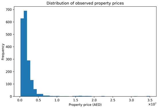
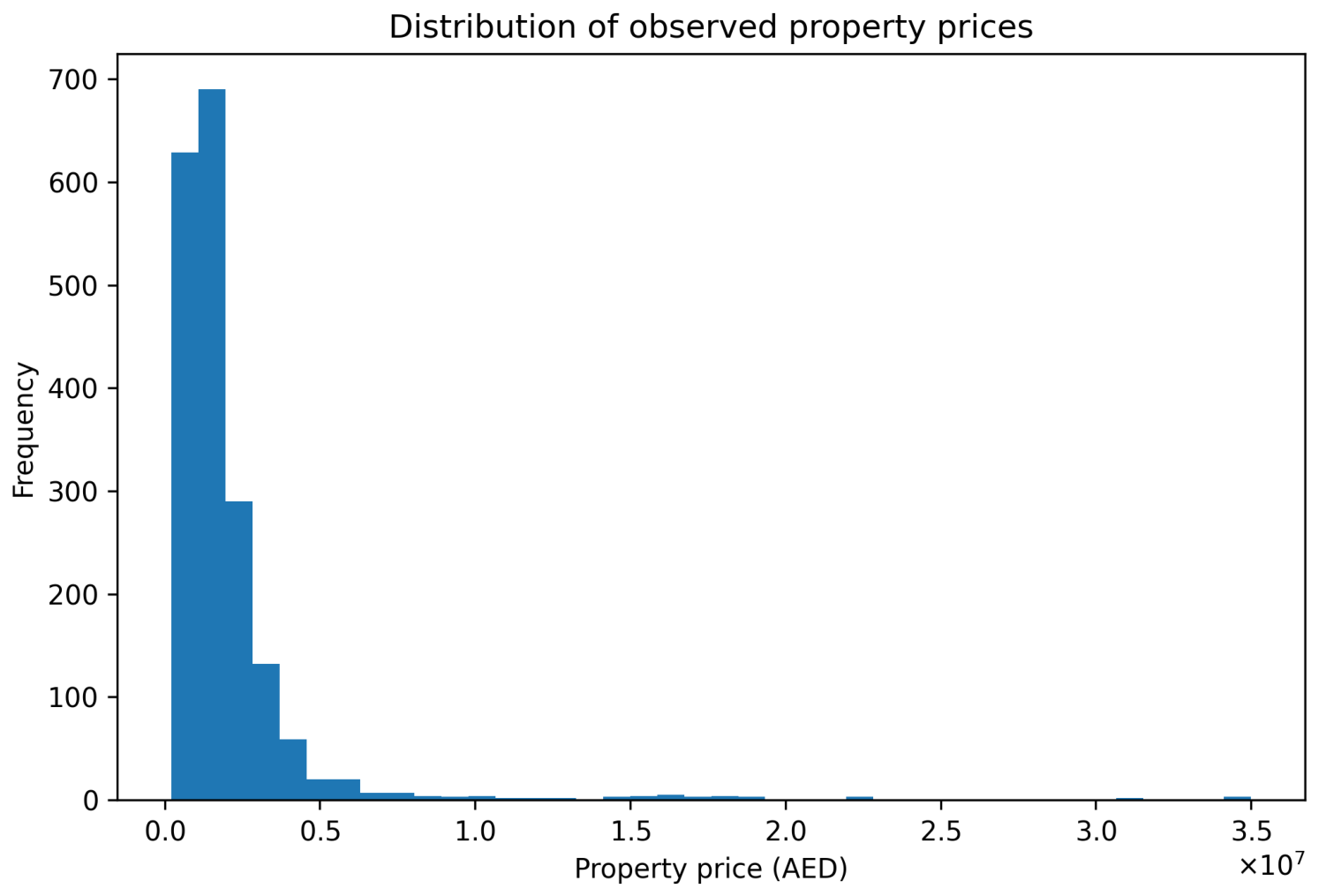
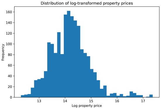
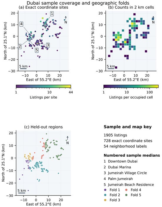
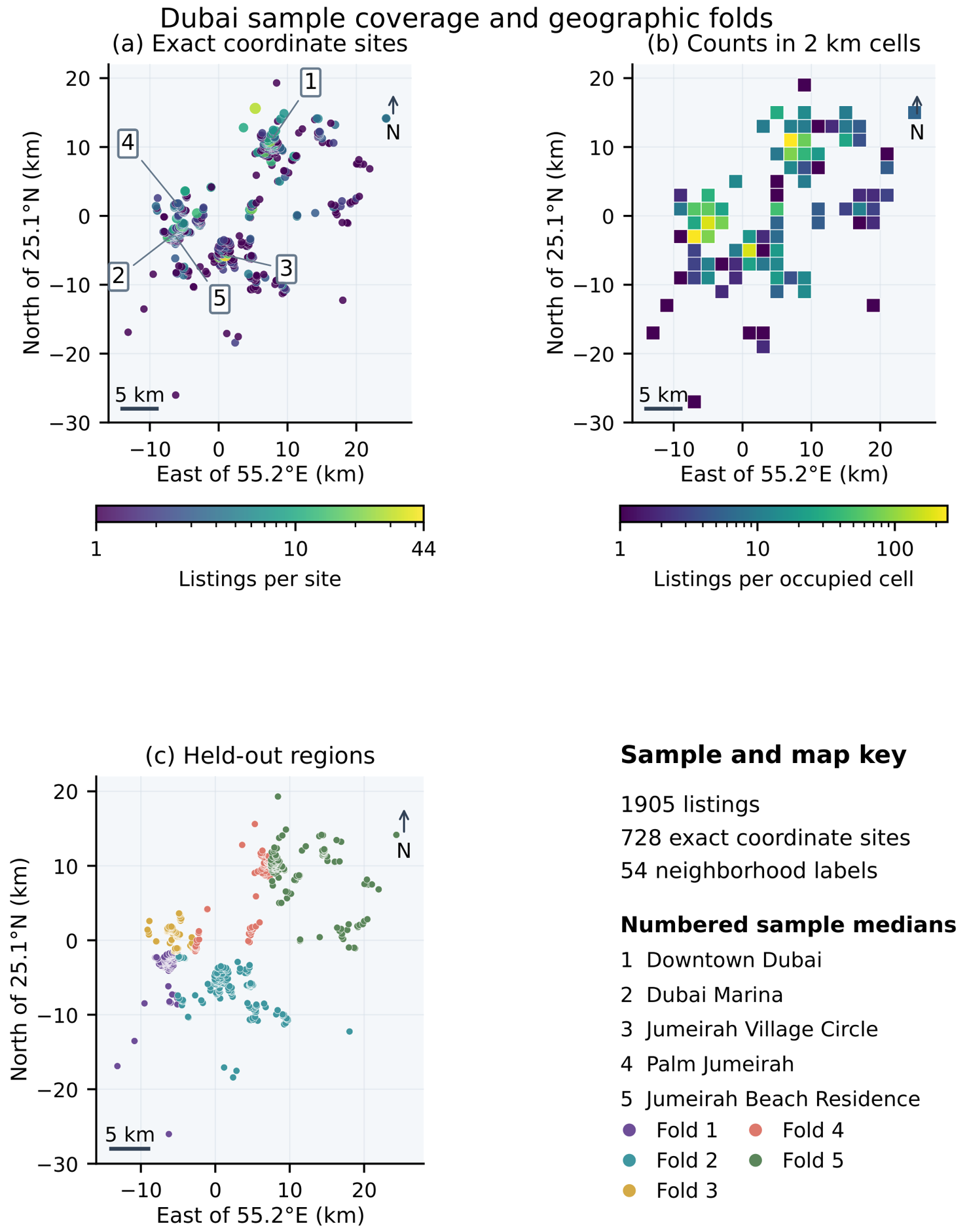
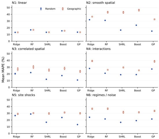
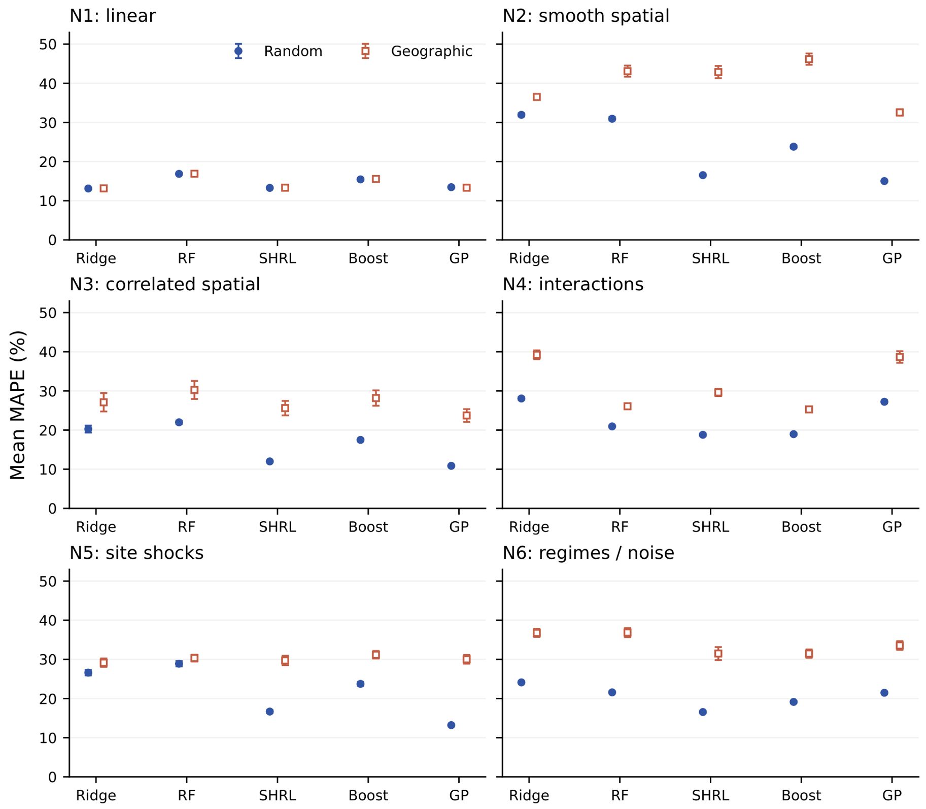
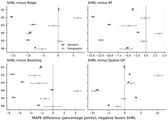
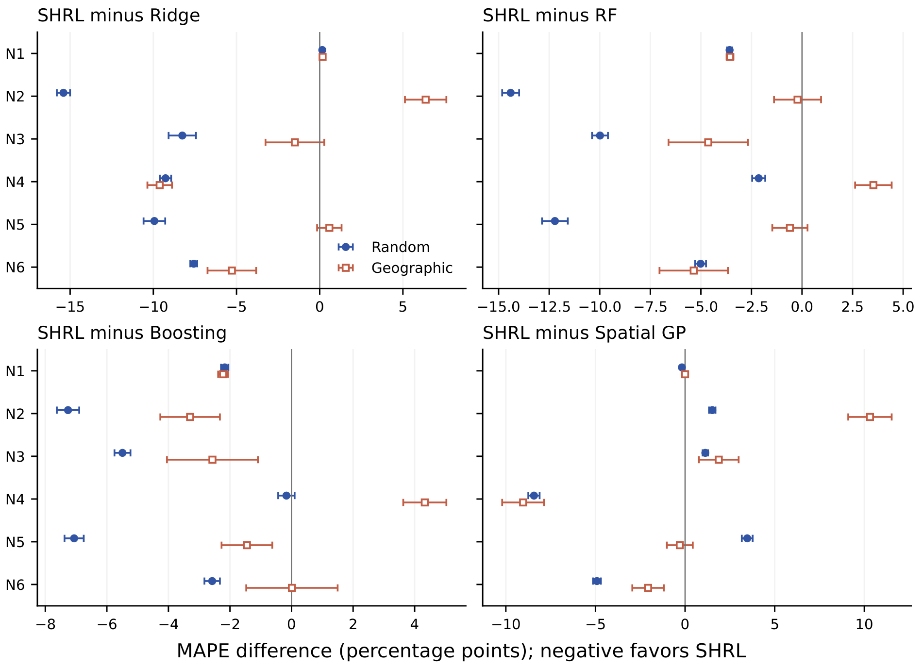
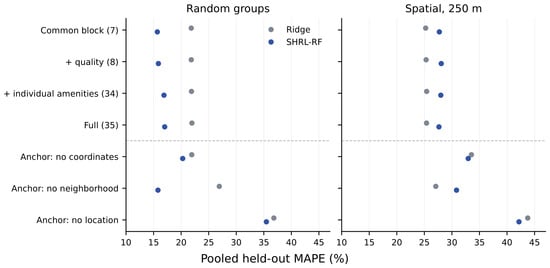
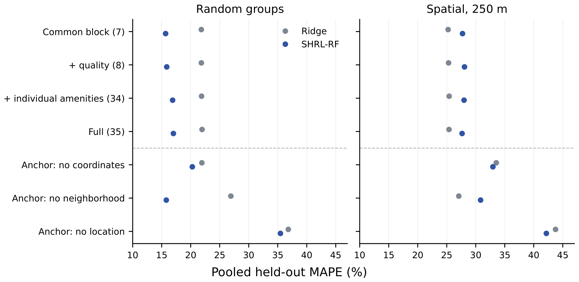
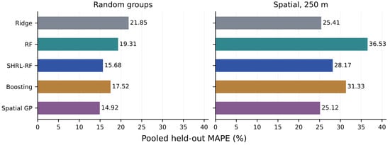
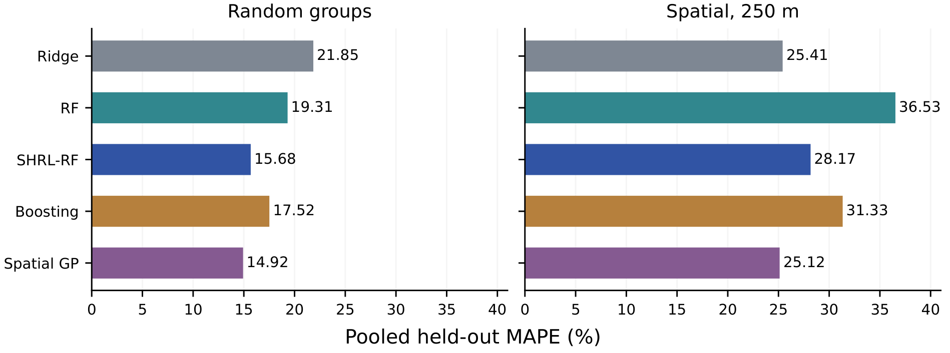
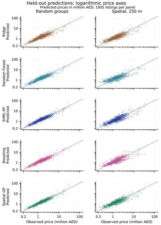
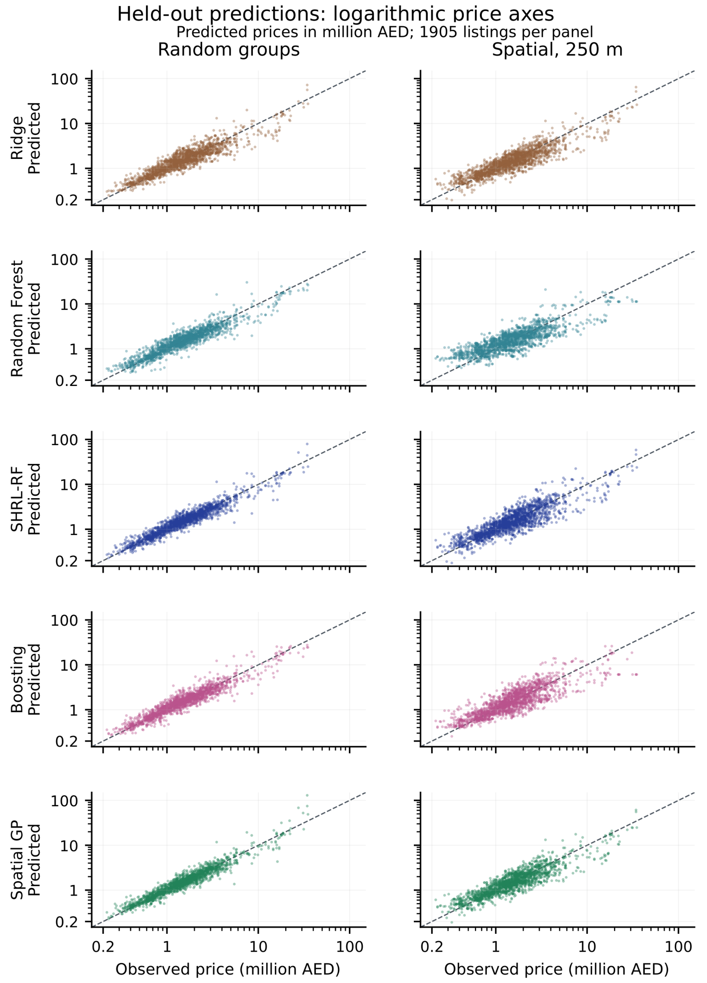
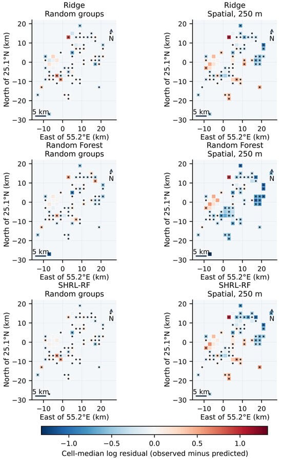
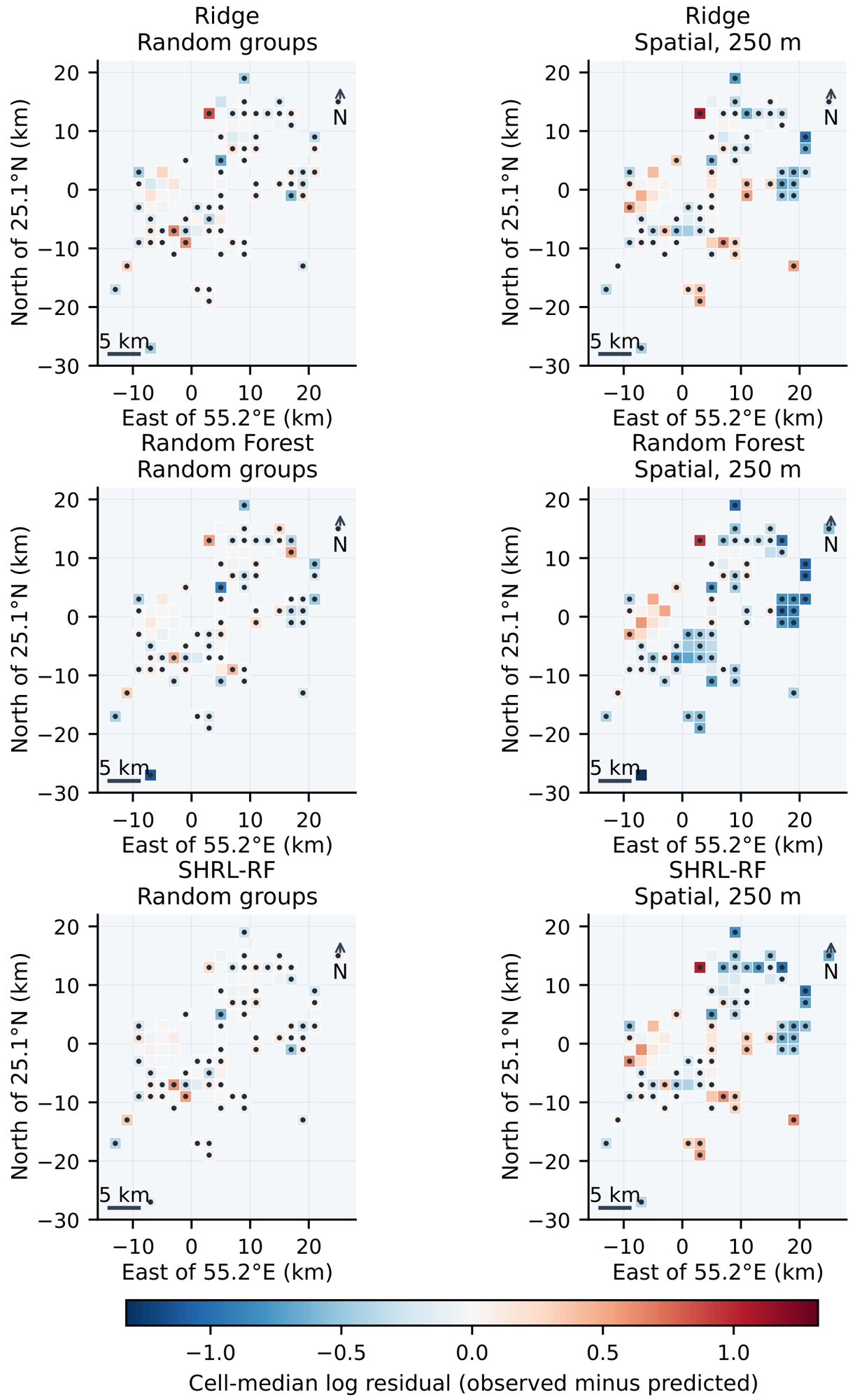
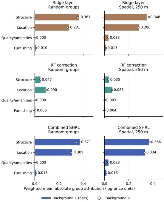
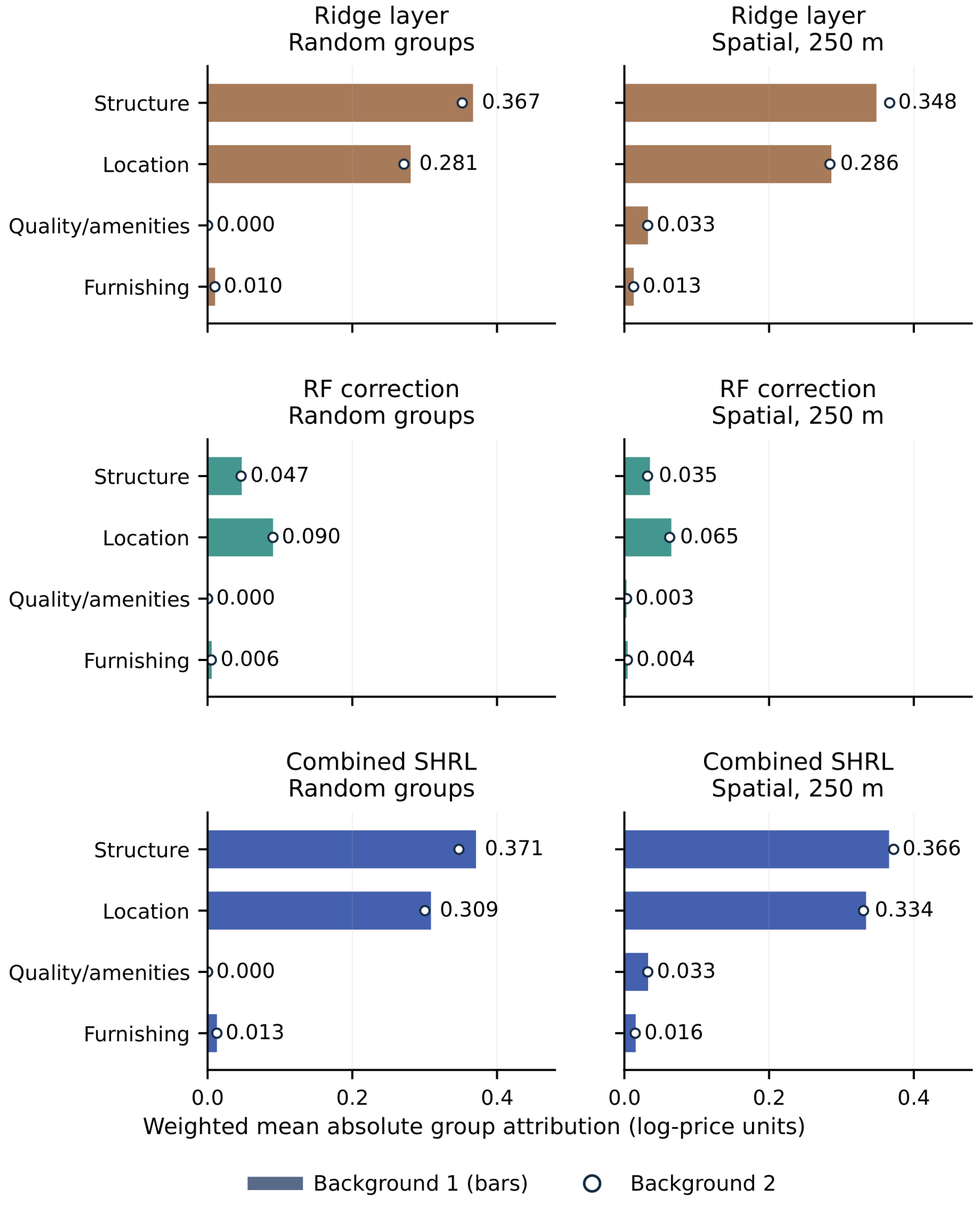
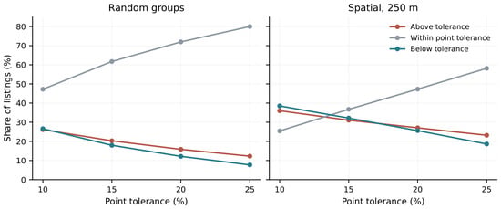
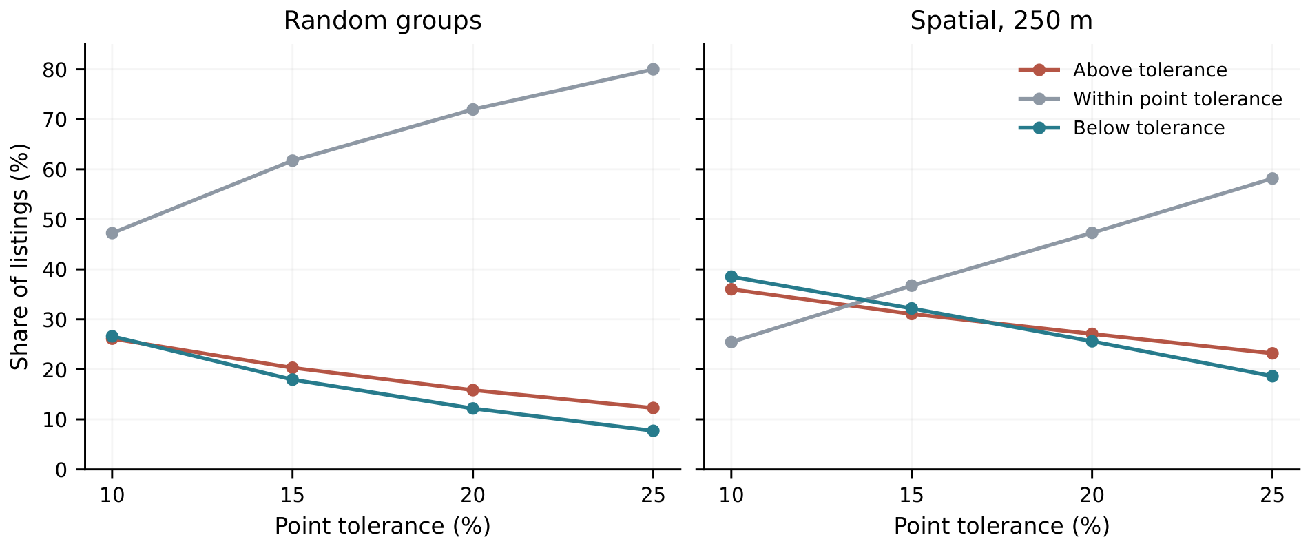
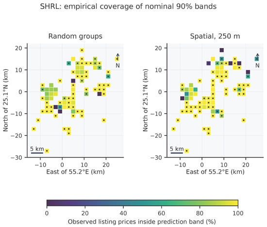
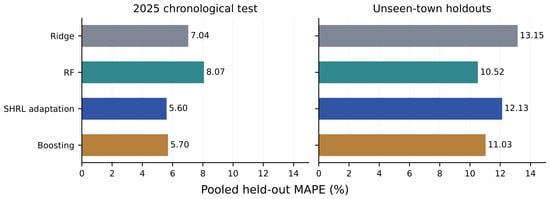

Disclaimer/Publisher’s Note: The statements, opinions and data contained in all publications are solely those of the individual author(s) and contributor(s) and not of MDPI and/or the editor(s). MDPI and/or the editor(s) disclaim responsibility for any injury to people or property resulting from any ideas, methods, instructions or products referred to in the content. |
© 2026 by the authors. Licensee MDPI, Basel, Switzerland. This article is an open access article distributed under the terms and conditions of the Creative Commons Attribution (CC BY) license.