Assessing Online Change Point Detection in Noisy Environments: A Case Study on Synthetic and Real Crime Data ^†

Abstract

This study benchmarks 16 online change point detection algorithms on both synthetic and real-world time series. The synthetic benchmark evaluates performance under controlled combinations of noise level, change magnitude, and change type, whereas the real-world benchmark uses manually labeled crime count series from multiple regions. The results show that no single method dominates across all scenarios. Under low-noise conditions, ssm_canary and ocpdet_two_sample_test achieve the strongest performance, whereas under high-noise conditions, changepoint_online_gaussian and ocpdet_two_sample_test are more competitive. In the real crime dataset, the best F1 scores are approximately 0.41, suggesting that current methods still have limited accuracy for operational crime monitoring. Overall, the findings show that the effectiveness of online change point detection depends strongly on the interaction between noise, change magnitude, and change type, and they provide practical guidance for selecting algorithms under different data conditions.

1. Introduction

Change point detection refers to the identification of structural changes in the behavior of a time series. Depending on the application setting, the detection approach can be either online or offline. Online methods process observations sequentially and aim to detect changes as new data arrive, whereas offline methods may analyze an entire observed sequence to identify change points retrospectively [1]. Online change detection has gained increasing relevance due to the rapid growth of streaming data generation across diverse domains [2]. Recent advances in online detection algorithms have contributed to addressing important issues, such as fuel leakage detection [3], identifying change points in virus spread [4], and localizing pipe bursts in water distribution networks [5], among others.

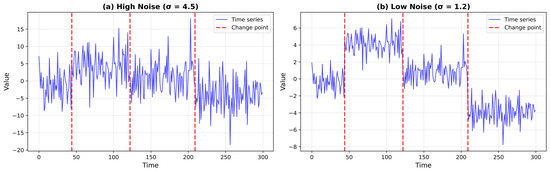
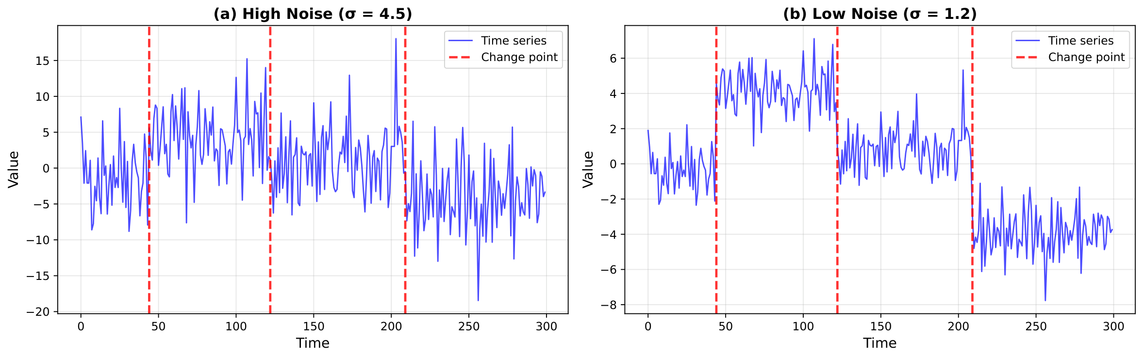
When a time series exhibits a high level of noise, change point detection methods may perform poorly [6], making the identification of change points challenging [7]. This problem becomes even more pronounced when the changes are subtle [3], sometimes making them difficult to detect even for humans. For example, Figure 1 shows two versions of a time series: one with high noise ($\sigma =4.5$) and another with low noise ($\sigma =0.2$). While the change points are clearly visible in the low-noise scenario, they become significantly harder to identify in the high-noise version, illustrating the challenges faced by automated algorithms and even human analysts. Moreover, noise may lead to false detections when no real change is present. Although noise is known to influence the performance of change detection algorithms, to the best of our knowledge, there is no systematic benchmarking of how these algorithms perform under different noise levels in settings with both weak and strong change points. Therefore, the present study analyzes how commonly used online change detection algorithms behave under varying levels of noise and change magnitude. The findings help guide the selection of appropriate detection methods depending on the characteristics of the time series under study, and they also open new research questions on how to improve change point detection in noisy environments.

Figure 1. Comparison of change point detection difficulty under different noise conditions. Both panels show time series with three change points (red dashed lines), but with different noise levels.

As a second objective, this research examines a real-world scenario in which noise affects time series, specifically the task of detecting change points in crime occurrences. Although this task can support crime monitoring, help identify regions with shifts in criminal activity, and inform policing strategies, it has received limited attention in the literature [8]. Moreover, crime-related time series typically exhibit high levels of noise, which hinders accurate change point detection. This noise arises not only from the inherent stochasticity of criminal behavior but also from structural biases in data collection, as crime statistics depend on citizens’ willingness to report incidents. In summary, the main contributions of this manuscript are as follows:

• A novel benchmarking analysis of the performance of online change point detection algorithms under varying noise levels and change magnitudes. To the best of our knowledge, this is the first study that systematically examines algorithmic behavior across such conditions.
• A performance evaluation of change point detection algorithms in a real-world scenario where noise strongly affects the time series, specifically crime count data.
• A new labeled dataset for detecting change points in crime-related time series.

2. Literature Review

Recent studies have addressed the problem of online change point detection. In [9], Cakmak et al. compared eight approaches (six published baselines plus two modified variants) for change point detection in cardiovascular time series data. In [10], a benchmarking of popular algorithms was conducted using simulated data and 37 real time series from various application domains. Ref. [11] evaluated online change point detection algorithms that operate on unbounded data streams with constant time and space complexity. Other authors, instead of comparing existing methods across different contexts, have developed new proposals for online change point detection, such as [3,7,12]. In [3], the authors proposed a novel memory-based online change point detection (MOCPD) framework to detect fuel leakage delays. Ref. [7] introduced a method called Delta Point, which divides the time series into intervals of user-specified, domain-specific length within which a suspected change point may be contained. In [12], the method requires no prior distributional knowledge of the time series and uses Information Gain to verify each new candidate change point score. In both the studies that benchmark existing methods and those that propose new approaches, there is no evaluation of algorithmic performance as a function of noise level or change point magnitude. Therefore, there is a lack of knowledge about how these algorithms behave under specific circumstances.

Regarding the detection of changes in crime event patterns, only a few studies have examined their effectiveness, even though applying change point detection algorithms can support police monitoring of criminal activity. For instance, Ref. [8] investigated the effectiveness of both online and offline change point detection methods for identifying critical changes in crime-related time series from the Boston and London Police Records datasets, finding that BOCPD achieved the best performance. In [13], the authors proposed a fuzzy approach to detect change points in the CICOP dataset (real-world crime data), consisting of 32 monthly time series. They concluded that the proposed method has strong potential for crime analysis; however, no comparisons with baselines or alternative methods were provided. The work in [14] presents a framework for detecting change points in terrorism-related time series, concluding that it could serve as an alternative approach for identifying links between terrorism and online activity.

3. Methods

This section describes the methodology used to benchmark online change point detection algorithms. The experimental design consists of two complementary evaluation components: (1) controlled experiments using synthetic time series with known ground-truth change points, and (2) real-world evaluation using manually labeled crime occurrence data.

3.1. Datasets

We use both synthetic and real-world datasets. The synthetic time series were designed to evaluate algorithmic performance under controlled conditions that are difficult to find in real labeled datasets (all code, datasets, and experimental configurations are available at https://github.com/AllanDBB/online-cpd-pipeline (accessed on 1 August 2026)).

3.1.1. Synthetic Time Series (Benchmark 1)

We generated synthetic time series across eight scenarios defined by the combination of two noise levels (high and low), two change point magnitudes (high and low), and two change point types (mean and slope). In total, 360 time series were produced, with 45 per scenario. The series were generated with lengths $L\in \{200,300,400\}$ and with $cp\in \{1,2,3,4\}$ change points.

Let $y_t$ denote the original observation and ${\tilde{y}}_t$ the perturbed observation. Noise was added according to

$${\tilde{y}}_t=y_t+{ϵ}_t,$$

(1)

where noise was sampled from a scaled standard normal distribution:

$${ϵ}_t=\sigma z_t,z_t\sim \mathcal{N}(0,1),$$

(2)

allowing the perturbation intensity to be controlled by $\sigma$. High-noise settings used $\sigma \in [3,6]$, whereas low-noise settings used $\sigma \in [0,0.3]$.

The magnitude of each change point is determined by a coefficient $\alpha$, applied over a randomly selected duration exceeding five time steps. High-magnitude changes used $\alpha \in [3,6]$, while low-magnitude changes used $\alpha \in [0.3,1.0]$.

For mean shifts, $\alpha$ was added directly to the time series. For slope shifts, the change was introduced gradually across the selected duration:

$$y_t={\displaystyle \frac{t}{n-1}}·\alpha ,t=0,1,\dots ,n-1.$$

(3)

3.1.2. Real-World Crime Data (Benchmark 2)

We manually labeled change points in 49 crime count time series from regions in Boston (4 series), Los Angeles (10 series), Chicago (14 series), and Costa Rica (21 series). Both daily and monthly series were used, and each was truncated to 120 time steps to facilitate consistent visual identification of change points. In total, 32 time series contain at least one labeled change point, while 17 contain none and serve as negative examples to assess specificity.

To characterize noise, we computed the Noise-to-Signal Ratio (NSR) for all 49 series after detrending and standardization. NSR spans 0.04 to 2.72 (median = 0.62, mean = 0.93, $\sigma$ = 0.73). We computed the Euclidean distance between each crime time series and the centroids of the synthetic time-series groups, using NSR and the magnitude of change as metrics. Based on the smallest distance to these groups, we classified each crime time series according to its noise level and magnitude of change. The classification assigns 33 series to the high-noise group (mean NSR = 1.26, $\sigma$ = 0.66) and 16 to low-noise (mean NSR = 0.25, $\sigma$ = 0.12), a 5.1× separation. Table 1 summarizes the distribution of the 49 series by noise group and change magnitude, with “no change” indicating series without labeled change points.

Table 1. Distribution of crime time series by noise level and change magnitude (N = 49) using centroid-based noise labels; “no change” denotes series without labeled change points.

Noise Level	High Change	Low Change	No Change	Total
High noise (synthetic centroid)	15 (31%)	1 (2%)	17 (35%)	33 (67%)
Low noise (synthetic centroid)	11 (22%)	5 (10%)	0 (0%)	16 (33%)
Total	26 (53%)	6 (12%)	17 (35%)	49 (100%)

3.2. Algorithms

We evaluated 16 online unsupervised change point detection algorithms spanning multiple methodological families:

• Statistical Process Control: Page-Hinkley (PH, page_hinkley_river) [15], Adaptive Windowing (ADWIN, adwin_river) [16], Exponentially Weighted Moving Average (EWMA, ewma_numpy), Cumulative Sum (CUSUM, ocpdet_cumsum) [17].
• Segmentation-Based Methods: Kernel PELT with a radial basis function cost (Focus RBF, changepoint_online_focus), Gaussian-likelihood PELT (Gaussian L2, changepoint_online_gaussian), non-parametric sliding-window comparison (NPFocus, changepoint_online_np_focus), and a multivariate Mahalanobis-distance extension (MDFocus, changepoint_online_md_focus).
• State-Space Models: Basic Kalman Filter tracking residuals (SSM-Canary, ssm_canary) [18], Tractable Approximate Gaussian Inference with LSTM-based adaptive state modeling (TAGI-LSTM, tagi_lstm_ssm), and Robust Square-Root Kalman Filtering with outlier handling (SKF-Canary, skf_kalman_canary) [18].
• Bayesian Methods: Bayesian Online Change Point Detection with a Student’s t predictive distribution (BCPD CPFinder, ocpdet_ewma) [19].
• Neural Network-Based Methods: Autoregressive MLP monitoring prediction residuals (OCPDet-Neural, ocpdet_neural_networks), and neural density-ratio estimation using RuLSIF (RuLSIF-Roerich, rulsif_roerich) [20].
• Two-Sample Testing: Sliding-window Kolmogorov–Smirnov test (Two-Sample KS, ocpdet_two_sample_tests), and Sequential Discounting Autoregression with outlier scoring (ChangeFinder, changefinder_sdar) [21].

All algorithms were implemented using their corresponding reference libraries (e.g., River [22], Ruptures [23], OCPDet [10]).

3.3. Performance Metrics

Following standard practice in time series change point detection [10], we use the F1-score with a tolerance window $\delta =10$ to account for detection delays:

$${\mathrm{F}1}_{\delta }={\displaystyle \frac{2·{\mathrm{Precision}}_{\delta }·{\mathrm{Recall}}_{\delta }}{{\mathrm{Precision}}_{\delta }+{\mathrm{Recall}}_{\delta }}}.$$

(4)

It is worth noting that the implications of $\delta =10$ differ across temporal scales: for daily series it corresponds to ten days, whereas for monthly series it spans nearly one year. We retain a uniform $\delta$ to enable consistent cross-series comparison, acknowledging that operational interpretations may vary by granularity.

3.4. Experimental Procedure

For each of the eight synthetic scenarios, we randomly split the time series into 70% for calibration and 30% for testing. A grid search was performed on the calibration partition for each algorithm, selecting the hyperparameters that maximized the F1-score. These configurations were then used to evaluate performance on the test partition. For the Real-World Crime Dataset, we followed the same procedure, but without scenario-based grouping.

4. Results

4.1. Benchmark 1: Synthetic Data Performance

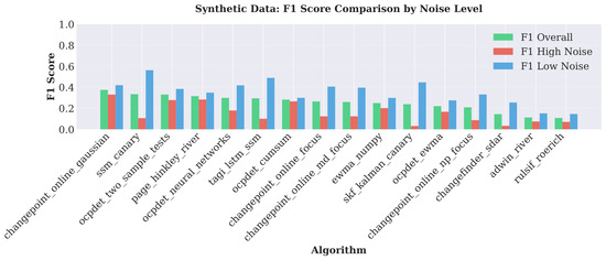
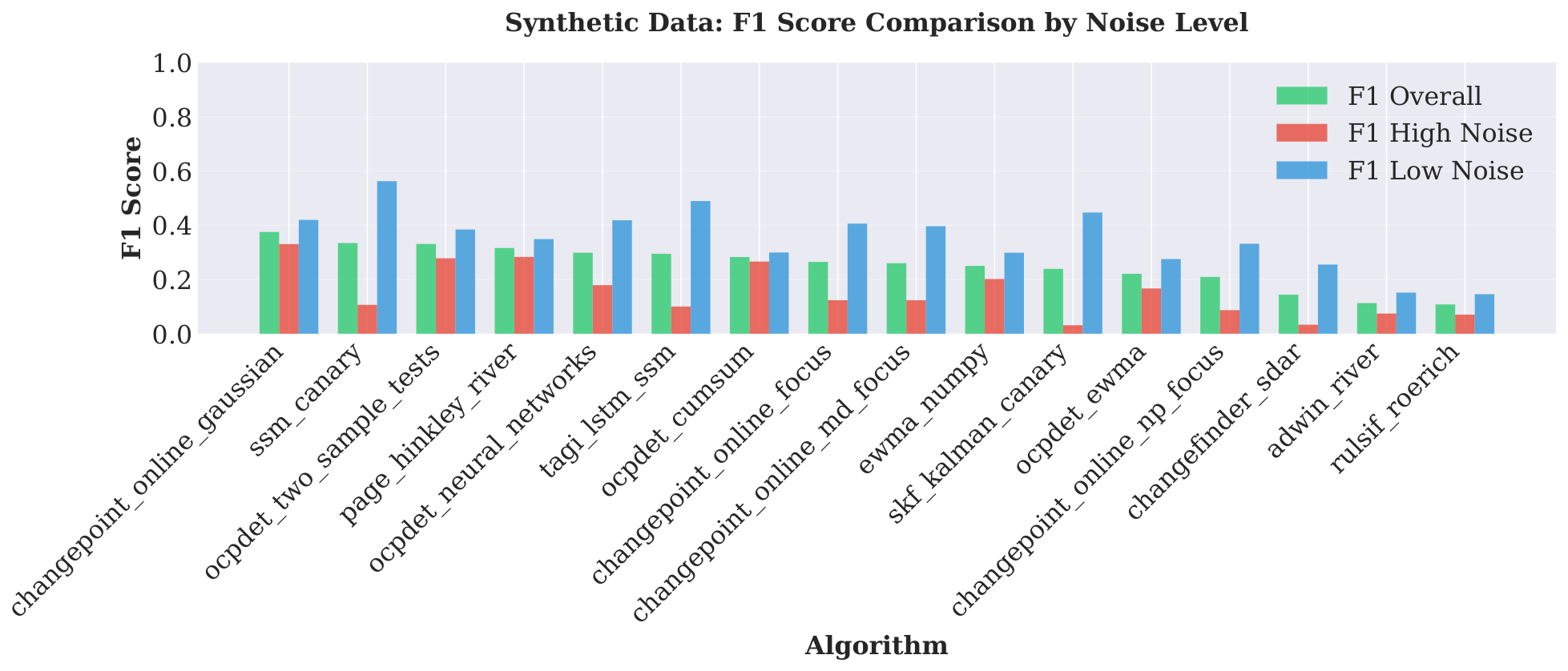
Figure 2 shows the average F1-score across all general conditions. The results indicate that the best overall performer is changepoint_online_gaussian, with an F1-score of 0.38, followed by ssm_canary, which achieves an F1-score of 0.34. When performance is analyzed by noise level, the results show that under high-noise conditions, changepoint_online_gaussian remains the top-performing method, attaining an F1-score of 0.33. In contrast, under low-noise conditions, ssm_canary yields the highest performance, reaching an F1-score of 0.565.

Figure 2. Synthetic data: Multi-metric performance comparison for all 16 algorithms. Algorithms ordered by descending average F1 score.

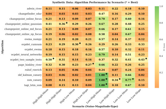
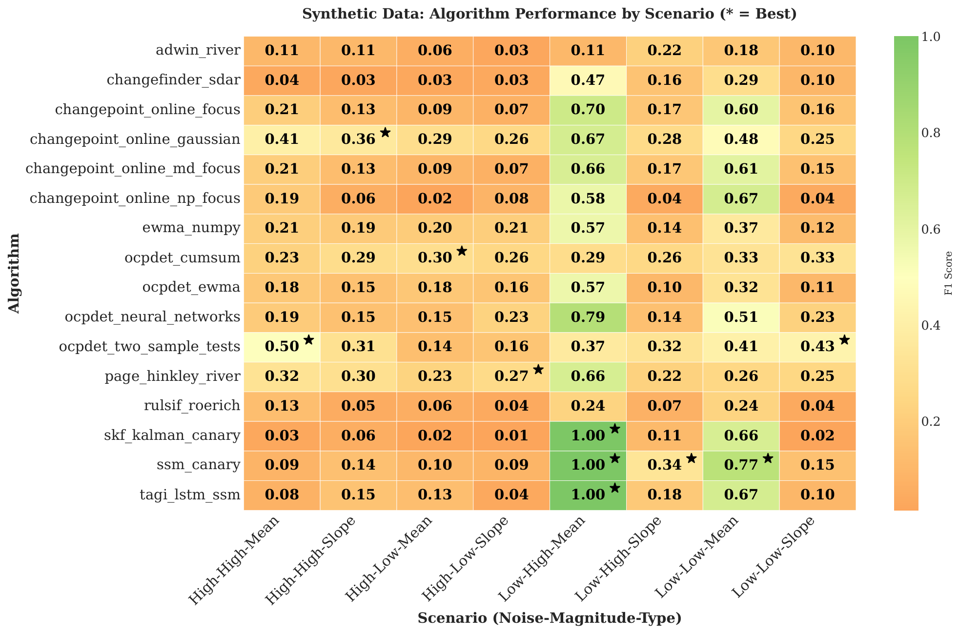
Figure 3 shows the performance of all algorithms across each specific scenario. Stars (*) indicate the best-performing method in each case. The results reveal that no single algorithm consistently outperforms the others across the eight evaluated conditions. For example, under high noise and high-magnitude slope change points, the top performer is changepoint_online_gaussian, whereas under high noise and high-magnitude mean change points, the best-performing method is ocpdet_two_sample_tests. Regarding the low noise, of the four low-noise algorithms, the best-performing is ssm_canary. However, when the magnitude of the slope change point is low, ssm_canary performs poorly, and the best alternative becomes ocpdet_two_sample_tests.

Figure 3. Synthetic data performance heatmap: F1 scores for all 16 algorithms across 8 scenarios. Stars (*) in top-right corners indicate best performers per scenario (multiple stars for ties). Color intensity reflects detection quality (green = high, red = low). Scenario notation: Noise–Magnitude–Type (e.g., Low–Low–Step, High–High–Ramp).

As expected, change-point detection is substantially more effective when noise levels are low. Most algorithms tend to show better performance in low-noise scenarios. In addition, in three of the low-noise scenarios, the best algorithm outperformed the best algorithm in the high-noise scenarios.

Another important observation is that, under high noise, the performance gap between detecting changes in the mean and in the slope is relatively small for most algorithms. In contrast, when noise levels are low, notable differences emerge across algorithms depending on the type of change point. This finding suggests that high noise degrades detection performance regardless of the change type or magnitude.

4.2. Benchmark 2: Real Crime Data Performance

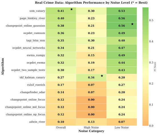
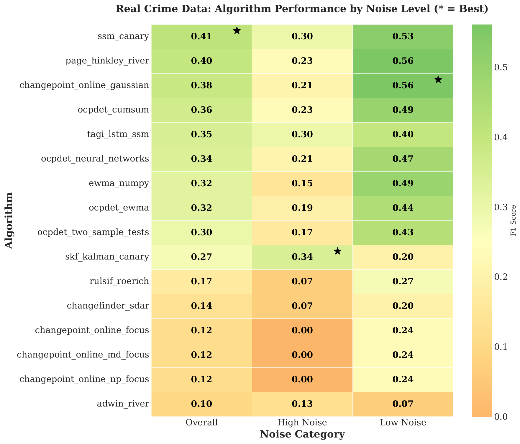
Figure 4 shows the performance of the algorithms on the real crime dataset, stratified by the centroid-based noise labels. The overall performance reveals patterns that align with the findings from the synthetic dataset. The three best-performing algorithms in the real dataset—ssm_canary (0.41), page_hinkley_river (0.40), and changepoint_online_gaussian (0.38)—were also among the top-performing algorithms in the synthetic dataset. When examining performance by noise level, ssm_canary was not the best overall but ranked third, and for the low-noise level, it achieved second place. These findings indicate that ssm_canary is a good option for low-noise conditions, as was demonstrated with the synthetic dataset; however, unlike the synthetic study, it also performed well under high-noise conditions in the real data. A possible explanation is that the noise added to the synthetic time series was more aggressive than the noise present in the real time series.

Figure 4. Real crime data performance heatmap: F1 scores for 16 algorithms stratified by noise level (labels derived from synthetic centroids). Left column shows overall performance; middle and right columns show performance on high- and low-noise subsets. Stars (*) in top-right corners indicate best performer(s) per column.

The best overall F1 scores—approximately 0.41—are not encouraging if high accuracy in detecting changes in criminal activity is required. However, compared with the synthetic datasets, this performance exceeds that of most high-noise scenarios, as well as low-noise scenarios involving slope-based change points. The noise-level stratification highlights that the primary difficulty in crime data analysis stems from the high-noise subset, where even the best-performing algorithm achieves an F1 score of only 0.34.

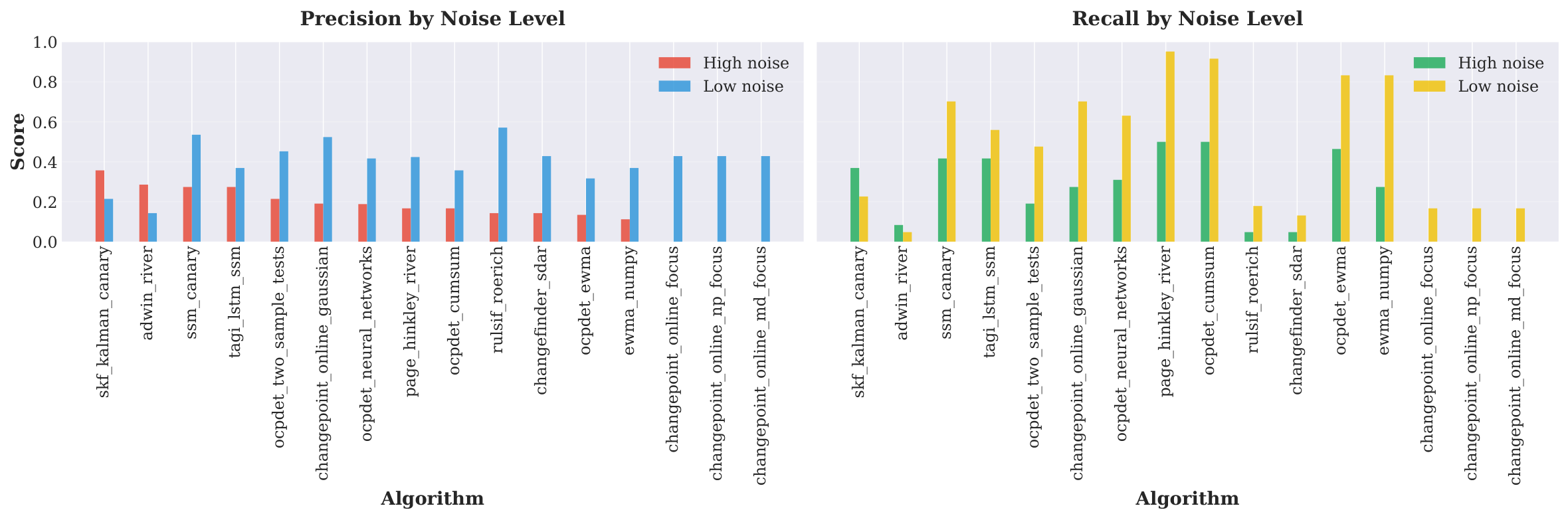
Finally, Figure 5 shows the precision and recall results for both low and high noise levels. One notable finding is that recall is much higher than precision, especially under low-noise conditions. This imbalance suggests that the algorithms tend to produce a large number of false alarms, which from an operational standpoint could lead to inefficient resource allocation in real-world crime monitoring contexts. It is also worth mentioning that the skf_kalman_canary algorithm achieves better recall and precision at high noise levels. The adwin_river algorithm also shows this pattern, although its overall performance remains low.

Figure 5. Precision and recall on real crime data by noise level (labels derived from synthetic centroids). Bars show mean precision and recall per algorithm, split into high-noise and low-noise subsets.

5. Conclusions

According to the results, no single algorithm consistently achieves the best performance across all scenarios. Nevertheless, several patterns emerge. The best option under low-noise conditions is ssm_canary, except when the magnitude of the change is small and the change point occurs in the slope. Under high-noise conditions, the most reliable choice is changepoint_online_gaussian. In one scenario, it was the top performer, and in two additional scenarios it produced results very close to the best-performing algorithm. The only exception arises when the change point corresponds to a high-magnitude shift in the mean. The analysis of the real crime dataset also reveals that ssm_canary and changepoint_online_gaussian are two of the best-performing options. However, ssm_canary demonstrates greater robustness across both high- and low-noise conditions. Our results suggest that algorithm selection should be guided primarily by the noise characteristics of the target data.

The findings also suggest that future research should focus on (i) improving change-point detection in high-noise time series, where all methods degrade sharply; (ii) handling slope-based changes, which remain challenging even in low-noise synthetic cases; and (iii) designing methods tailored to crime count data, since current algorithms do not yet provide sufficient accuracy for operational use.

References

- Aminikhanghahi, S.; Cook, D.J. A survey of methods for time series change point detection. Knowl. Inf. Syst. 2017, 51, 339–367. [Google Scholar] [CrossRef] [Scilit] [PubMed]
- Namoano, B.; Starr, A.; Emmanouilidis, C.; Carcel, C.R. Online change detection techniques in time series: An overview. In Proceedings of the 2019 IEEE International Conference on Prognostics and Health Management (ICPHM); IEEE: Piscataway, NJ, USA, 2019; pp. 1–10. [Google Scholar]
- Chu, R.; Chik, L.; Song, Y.; Chan, J.; Li, X. Real-time fuel leakage detection via online change point detection. Int. J. Data Sci. Anal. 2025, 20, 6583–6600. [Google Scholar] [CrossRef] [Scilit]
- Dehning, J.; Zierenberg, J.; Spitzner, F.P.; Wibral, M.; Neto, J.P.; Wilczek, M.; Priesemann, V. Inferring change points in the spread of COVID-19 reveals the effectiveness of interventions. Science 2020, 369, eabb9789. [Google Scholar] [CrossRef] [Scilit] [PubMed]
- Mzembegwa, T.; Nyirenda, C.N. Real-time pipe burst localization in water distribution networks using change point detection algorithms. In Proceedings of the 2024 International Conference on Emerging Trends in Networks and Computer Communications (ETNCC), Windhoek, Namibia, 23–25 July 2024; pp. 1–8. [Google Scholar]
- Chen, X.C.; Yao, Y.; Shi, S.; Chatterjee, S.; Kumar, V.; Faghmous, J.H. A general framework to increase the robustness of model-based change point detection algorithms to outliers and noise. In Proceedings of the 2016 SIAM International Conference on Data Mining, Miami, FL, USA, 5–7 May 2016; pp. 162–170. [Google Scholar]
- Gold, N.; Frasch, M.G.; Herry, C.L.; Richardson, B.S.; Wang, X. A doubly stochastic change point detection algorithm for noisy biological signals. Front. Physiol. 2018, 8, 1112. [Google Scholar] [CrossRef] [Scilit] [PubMed]
- Konstantinou, A.; Chatzakou, D.; Theodosiadou, O.; Tsikrika, T.; Vrochidis, S.; Kompatsiaris, I. Trend detection in crime-related time series with change point detection methods. In Proceedings of the International Conference of the Cross-Language Evaluation Forum for European Languages, Thessaloniki, Greece, 18–21 September 2023; pp. 72–84. [Google Scholar]
- Cakmak, A.; Reinertsen, E.; Nemati, S.; Clifford, G.D. Benchmarking changepoint detection algorithms on cardiac time series. arXiv 2024, arXiv:2404.12408. [Google Scholar]
- den Burg, G.J.J.V.; Williams, C.K.I. An evaluation of change point detection algorithms. arXiv 2020, arXiv:2003.06222. [Google Scholar]
- Wang, Z.; Lin, X.; Mishra, A.; Sriharsha, R. Online changepoint detection on a budget. In Proceedings of the 2021 International Conference on Data Mining Workshops (ICDMW), Auckland, New Zealand, 7–10 December 2021; pp. 414–420. [Google Scholar]
- Zameni, M.; Sadri, A.; Ghafoori, Z.; Moshtaghi, M.; Salim, F.D.; Leckie, C.; Ramamohanarao, K. Unsupervised online change point detection in high-dimensional time series. Knowl. Inf. Syst. 2020, 62, 719–750. [Google Scholar] [CrossRef] [Scilit]
- Albertetti, F.; Grossrieder, L.; Ribaux, O.; Stoffel, K. Change points detection in crime-related time series: An on-line fuzzy approach based on a shape space representation. Appl. Soft Comput. 2016, 40, 441–454. [Google Scholar] [CrossRef] [Scilit]
- Theodosiadou, O.; Pantelidou, K.; Bastas, N.; Chatzakou, D.; Tsikrika, T.; Vrochidis, S.; Kompatsiaris, I. Change point detection in terrorism-related online content using deep learning derived indicators. Information 2021, 12, 274. [Google Scholar] [CrossRef] [Scilit]
- Page, E.S. Continuous inspection schemes. Biometrika 1954, 41, 100–115. [Google Scholar] [CrossRef] [Scilit]
- Bifet, A.; Gavaldà, R. Learning from time-changing data with adaptive windowing. In Proceedings of the 2007 SIAM International Conference on Data Mining, Minneapolis, MN, USA, 26–28 April 2007; pp. 443–448. [Google Scholar]
- Page, E.S. Cumulative sum charts. Technometrics 1961, 3, 1–9. [Google Scholar] [CrossRef]
- Chen, M.; Tyler, D. Canary: A Python library for online change detection. Softw. Impacts 2021, 10, 100151. [Google Scholar]
- Adams, R.P.; MacKay, D.J.C. Bayesian online changepoint detection. arXiv 2007, arXiv:0710.3742. [Google Scholar]
- Liu, Y.; Yamada, S.; Sugiyama, M.; Murata, N. Change-point detection in time-series data by relative density-ratio estimation. Neural Netw. 2013, 43, 72–83. [Google Scholar] [CrossRef] [Scilit] [PubMed]
- Yamanishi, K.; Takeuchi, J. A unifying framework for detecting outliers and change points from non-stationary time series data. In Proceedings of the Eighth ACM SIGKDD International Conference on Knowledge Discovery and Data Mining, Edmonton, AB, Canada, 23–26 July 2002; pp. 676–681. [Google Scholar]
- Montiel, J.; Halford, M.; Mastelini, S.M.; Bolmier, G.; Sourty, R.; Vaysse, R.; Zouitine, A.; Gomes, H.M.; Read, J.; Abdessalem, T.; et al. River: Machine learning for streaming data in Python. J. Mach. Learn. Res. 2021, 22, 1–8. [Google Scholar] [CrossRef] [Scilit]
- Truong, C.; Oudre, L.; Vayatis, N. Selective review of offline change point detection methods. Signal Process. 2020, 167, 107299. [Google Scholar] [CrossRef] [Scilit]
Disclaimer/Publisher’s Note: The statements, opinions and data contained in all publications are solely those of the individual author(s) and contributor(s) and not of MDPI and/or the editor(s). MDPI and/or the editor(s) disclaim responsibility for any injury to people or property resulting from any ideas, methods, instructions or products referred to in the content. |
© 2026 by the authors. Licensee MDPI, Basel, Switzerland. This article is an open access article distributed under the terms and conditions of the Creative Commons Attribution (CC BY) license.