SimDSL: A Domain-Specific Language for Large-Scale GPU-Resident Simulation

Abstract

We present SimDSL, a domain-specific language (DSL) for executing large-scale simulations on the GPU using an Entity Component System (ECS) architecture. Systems written in SimDSL are analyzed, lowered into an intermediate representation, and compiled by a CuPy-based backend into CUDA kernels operating over structure-of-arrays archetype tables. We evaluate SimDSL on five workloads: Particle Fountain, Traffic Ring, Reaction Diffusion, Ant Colony, and Tower Defense. The evaluation compares SimDSL with straightforward CuPy and CUDA baseline implementations under matched simulation configurations. Results show that SimDSL sustains GPU-resident execution and achieves favorable performance relative to these baselines. These findings demonstrate that high-level ECS simulation programs can be compiled into efficient GPU execution without requiring users to manually implement and coordinate low-level kernels.

1. Introduction

Large-scale simulation is a core computational tool in scientific computing, engineering, robotics, interactive systems, and machine learning. Many modern workloads require tracking and updating large populations of heterogeneous objects, such as particles, vehicles, agents, cells, or game entities, under shared spatial and temporal rules. In such settings, performance depends not only on the cost of individual updates, but also on how efficiently the simulation scales as the number of active objects grows. GPUs are an attractive target for these workloads because they offer massive parallel throughput and high memory bandwidth. However, exploiting GPUs effectively remains difficult when a simulation is expressed at a high level of abstraction and includes dynamic object state, heterogeneous data, and irregular structural changes [1].

Entity Component System (ECS) programming is an appealing model for object-centric simulation because it separates state into components and behavior into systems, and naturally encourages data-oriented organization. Although ECS is widely known from game-engine design, its underlying structure is also well suited to large-scale simulation: entities can be stored in structure-of-arrays layouts, systems correspond to bulk operations over large populations of entities, and queries define regular access patterns over subsets of entities. These properties make ECS a promising abstraction for scalable simulation [2,3,4]. In practice, however, most ECS frameworks are designed primarily as software architecture tools rather than as compilation targets for high-performance execution. Developers often face an undesirable tradeoff: either preserve a high-level ECS formulation and accept limited scalability, or rewrite the simulation as low-level backend-specific code.

Bridging this gap is nontrivial. The same abstractions that make ECS expressive also complicate efficient execution. (1) Entities are heterogeneous and may migrate across archetypes as their component sets change. (2) Systems are written as high-level queries over subsets of entities rather than as explicit kernels over flat arrays. (3) Structural operations such as spawning, destroying, adding, and removing components introduce synchronization and data-movement requirements that do not map directly to bulk-synchronous execution. Efficient support for ECS simulation therefore requires more than a straightforward translation of system code. It requires a compilation model that recovers access structure from high-level systems, preserves schedule semantics, maps queries to backend-executable programs, and coordinates staged structural updates across execution backends.

In this work, we present an embedded ECS DSL for simulations that supports a GPU backend while maintaining a unified high-level programming model. Our approach treats ECS as a domain-specific simulation language rather than merely a software framework. Systems written in the DSL are analyzed to recover their query structure, component and resource accesses, and staged structural effects. They are then lowered through a sequence of intermediate representations that make execution semantics, dependencies, and schedule boundaries explicit. From this shared representation, the compiler constructs backend execution plans for the GPU runtime. On the GPU, execution is organized around device programs, backend specialization, and a persistent resident runtime with staged synchronization of structural updates.

This approach has two benefits. From a software perspective, it allows developers to describe simulation behavior once in a modular ECS form while retaining a path to backend-specific acceleration. From a systems perspective, it provides a structured compilation and runtime model for object-centric simulation workloads whose execution depends on both dense data traversal and explicit management of structural change. This is particularly relevant in settings where simulation is invoked repeatedly inside optimization, control, or learning loops, and where the ability to preserve a high-level programming model while still scaling execution is valuable.

SimDSL sits between ECS authoring frameworks and GPU kernel frameworks: it retains ECS structure and staged mutation as first-class constructs, while compiling them to GPU-resident, archetype-specialized execution rather than host-driven or purely array-based simulation. This work makes the following contributions:

1.

We design SimDSL, a Python-embedded ECS DSL for GPU simulation that unifies systems, queries, typed data access, and staged structural effects (spawn, destroy, and component transitions) under one authoring model. Unlike CPU-oriented ECS frameworks, which treat scheduling and structural mutation as host-side concerns, and unlike array-centric GPU frameworks (e.g., Taichi, JAX), which lack first-class ECS queries and archetype lifecycles, SimDSL exposes ECS semantics as the programming interface while targeting GPU-resident execution.

2.

We develop an analysis and lowering pipeline that extracts authored systems into an intermediate representation, validates host/device schedule constraints, and compiles them into group-ordered execution plans. The pipeline separates ECS intent (queries, access modes, and structural effects) from backend code generation, enabling archetype-specialized kernel emission rather than requiring authors to hand-manage SoA layouts, launches, and synchronization.

3.

We implement a CuPy-based runtime for archetype-oriented, GPU-resident ECS simulation. The runtime keeps simulation state on device across steps, applies deferred structural updates between schedule groups for stable iteration, and uses archetype-specialized kernels with launch-time binding of resources and buffers. This combination preserves ECS structural dynamics without forcing per-step host round-trips that dominate conventional ECS-on-GPU ports.

4.

We evaluate SimDSL on five representative workloads against matched straightforward CuPy and CUDA baselines. The study quantifies the cost of ECS abstraction relative to these GPU implementations and isolates the benefit of GPU residency under structural and non-structural simulation patterns.

The rest of the paper is organized as follows. Section 2 discusses related work. Section 3 presents the overview of SimDSL. Section 4 describes the design and implementation of SimDSL. Section 5 presents optimization strategies. Section 7 evaluates the DSL on five simulations and compares its performance against baseline implementations.

2. Related Work

ECS decomposes programs into entities, components, and systems, where systems operate over the components of the queried entities. Recent work has moved beyond informal descriptions and provided formal semantic accounts of ECS execution. Redmond et al. introduce Core ECS, a calculus and denotational semantics that models ECS programs as schedules of systems over an entity-component association, making the interaction between scheduling, determinism, and concurrency explicit [5]. Complementary performance studies show that ECS behavior is strongly shaped by storage layout: archetype-based designs improve iteration throughput through contiguous storage, whereas sparse-set designs can reduce the cost of structural edits [3,6]. Subsequent work extends the formal treatment of archetype ECS and shows that its data organization, stable system execution, and controlled structural mutation also provide a suitable execution substrate for accelerated simulation [7]. This direction is further demonstrated through GPU-resident execution of archetype ECS, where component storage and system computation remain on the device while structural changes are coordinated at explicit synchronization boundaries [7]. Together, these results motivate ECS as a structured, analyzable programming model whose systems, queries, storage organization, and structural effects expose execution structure relevant for compilation.

The closest prior works come from high-performance simulation systems and robotics GPU simulators that combine data-oriented design with large-scale parallel execution. Madrona  [2] emphasizes extensible, data-oriented organization for many-world simulation and demonstrates the value of structuring simulation state and execution around throughput-oriented data layouts. Isaac Gym shows that keeping simulation and learning pipelines on the GPU can significantly increase throughput by avoiding repeated CPU-GPU transfers [8]. Isaac Lab extends this approach with a more modular and scalable simulation stack [9]. These systems establish GPU-resident simulation as an effective substrate for large-scale workloads, but they remain primarily framework-centric: users express logic through simulator APIs, tensor programs, and environment wrappers. In contrast, our work focuses on compiling simulation logic written in an ECS-structured DSL, preserving systems, queries, and schedules as first-class units for analysis and backend specialization.

Python has repeatedly been used as a productive front end for compiled or accelerated execution under staging or restricted compilation. Copperhead [10], Parakeet [11], and Numba [12] demonstrate that restricted or specialized subsets of Python can be translated to native CPU and/or GPU execution. TensorFlow Eager [13] combines imperative execution with staged graph construction, while HiPy [14] retains higher-level program semantics above a lower-level intermediate representation to support subsequent specialization and optimization. Systems such as Taichi, Triton, and Halide [15,16,17] similarly demonstrate how domain-specific programming abstractions can be lowered to specialized implementations without requiring users to express all backend details directly. These systems, however, target programming abstractions different from those required for entity-based simulation. Taichi primarily expresses numerical computation over dense and sparse fields, Triton provides abstractions for constructing GPU kernels, and Halide represents computations over multidimensional arrays with separately specified schedules. None provides ECS component queries, archetype-organized entity storage, ordered execution of ECS systems, or deferred ECS structural mutation as first-class language/runtime constructs. SimDSL instead adopts the ECS system as its primary simulation abstraction. Users express systems, queries, component accesses, and structural operations in Python 3.12.12, while the compiler and runtime lower these operations to GPU-resident execution.

A more closely related class of systems generates parallel programs from higher-level representations of data and computation. Delite [18] provides a compiler framework for performance-oriented domain-specific languages, using domain operations and parallel patterns to support optimization and code generation for heterogeneous execution. Futhark [19] is a functional data-parallel array language whose compiler transforms high-level array programs into efficient parallel implementations, including GPU code. DaCe [20] takes a data-centric approach through Stateful DataFlow multigraphs (SDFGs), an intermediate representation that makes data movement and dependencies explicit and supports transformations and code generation for heterogeneous architectures. These systems demonstrate that exposing data organization and parallel computation structure to a compiler can enable automatic generation and optimization of accelerator programs.

SimDSL follows this general principle of retaining high-level program structure for backend generation, but the structure exposed to its compiler is specific to ECS simulation. SimDSL represents systems, component and resource accesses, archetype queries, execution groups, and staged structural effects as compiler-visible information. During planning, queries are resolved to matching archetypes and systems are lowered to archetype-specialized structure-of-arrays kernels. Structural operations such as entity creation, destruction, and component-set transitions are staged and applied at execution-group boundaries rather than being performed during entity iteration. Thus, SimDSL’s distinction is not automatic GPU code generation itself, but the use of ECS execution and structural semantics as compiler-visible information for GPU lowering.

Table 1 summarizes the differences in programming abstraction and runtime support. It shows that SimDSL shares with Delite, Futhark, and DaCe the broader strategy of using high-level program structure to guide accelerator generation. The difference lies in the structure made explicit to the compiler. Delite exposes DSL operations and parallel patterns, Futhark exposes nested data-parallel array computation, and DaCe exposes dataflow and data movement. SimDSL instead exposes ECS systems, archetype queries, component accesses, execution groups, and staged structural effects. This allows GPU lowering to be specialized around the archetype-based execution model rather than around a general array, dataflow, or parallel-pattern representation.

Table 1. Comparison of representative GPU programming and program-generation systems with SimDSL. Entries describe first-class abstractions provided by the language or compiler rather than functionality that could be implemented manually by users.

System	Primary Abstraction	Data/Execution Model
Taichi	Fields/kernels	Dense and sparse fields
Triton	Tile-based execution	Tensors/blocked programs
Halide	Functions + schedules	Multidimensional array pipelines
Delite	DSL operations/parallel patterns	DSL IR + heterogeneous execution
Futhark	Data-parallel array programs	Nested parallel arrays
DaCe	Stateful DataFlow multigraph	Explicit dataflow and data movement
SimDSL	ECS systems + queries	Archetype SoA + ordered groups

Several ECS frameworks are widely used in practice. Bevy [21] provides a Rust ECS for the Bevy engine. EnTT [22] is a high-performance C++ ECS. Flecs [4] offers a C/C++ ECS with rich querying and scheduling. Specs [23] targets Rust game engines such as Amethyst. Apecs [24] explores ECS in Haskell. These systems typically keep simulation state and scheduling on the CPU and realize structural change through deferred command buffers or phase-local flushes: create/destroy and component edits are queued during system iteration and applied at well-defined boundaries so matching views remain stable. Our design is motivated by this ECS programming model—especially Flecs-style queries and staged structural updates—but targets a different execution setting.

This queue-then-apply organization also mirrors classical techniques for structural updates under SIMD and GPU execution. During a parallel compute phase, effectful topology changes are recorded in a deferred mutation queue—typically with atomic slot allocation so concurrent lanes can enqueue safely—and are committed only by a separate structural-apply or compaction pass at a barrier, preserving a stable layout for vectorized iteration. SimDSL follows that pattern in its compiled device path: kernels atomically reserve structural-command slots, and a post-group GPU apply pass updates archetype storage, live counts, and entity-index mappings.

Unlike these frameworks, SimDSL compiles ECS systems to a GPU-resident runtime in which archetype state remains on device across steps and staged structural commands are enqueued and applied in a GPU structural-apply pass at group boundaries, rather than through a host-centric ECS runtime.

Prior work establishes three important foundations: ECS provides a structured model of object-centric simulation, robotics simulators demonstrate the practical importance of GPU-resident execution, and staged Python compilation shows how high-level programs can be specialized for accelerators. Our work combines these strands in a different way. Rather than exposing only a simulator framework API or compiling isolated numerical kernels, we treat ECS itself as a domain-specific simulation language and compile systems, queries, and schedules into backend-specific execution plans while preserving a shared high-level programming model for GPU execution.

3. SimDSL Overview

SimDSL is an embedded Python domain-specific language for archetype-based Entity Component System simulation that also supports a companion dense-array programming model. Its design goal is to preserve a direct and lightweight programming interface while exposing enough semantic structure for staged execution, effect-aware compilation, and backend-specific planning. Programmers write ordinary Python functions together with typed schema declarations, but the implementation captures this structure through decorators, recovers the relevant data dependencies, and lowers the resulting program to a backend execution plan. The result is a single source-level programming model that can be specialized for GPU execution while preserving a consistent simulation semantics.

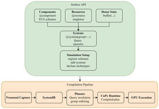
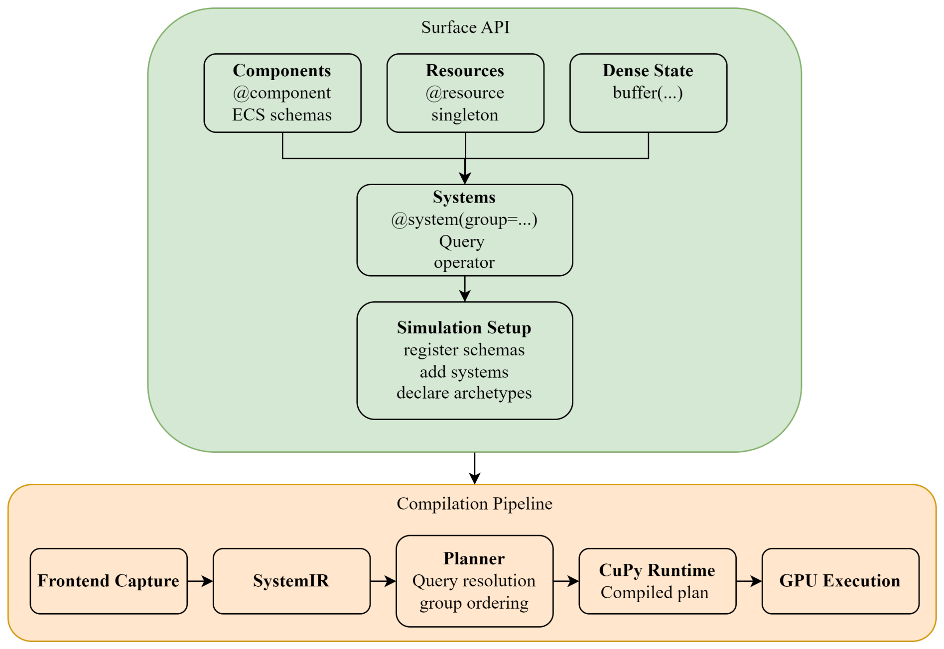
Figure 1 summarizes the architecture of SimDSL. The upper portion shows the surface programming model exposed to the simulation author, including schemas, systems, queries, groups, operators, and simulation setup. The lower portion shows the compilation and execution pipeline, from frontend capture and intermediate representation construction through planning, the CuPy runtime, and GPU execution.

Figure 1. Unified architecture of SimDSL. The upper portion shows the surface programming model exposed to the simulation author, while the lower portion shows the compilation and execution pipeline from frontend capture and intermediate representation construction through planning, the CuPy runtime, and GPU execution.

3.1. Programming Model

SimDSL provides a set of abstractions: components, resources, buffers, systems, queries, groups, and operators. Typed state is introduced through @component and @resource for ECS-oriented data and through buffer(…) for dense named arrays. Components represent per-entity state stored in archetypes, resources represent singleton global state, and buffers represent dense simulation state outside the archetype layout. Systems are ordinary Python functions annotated with @system, which attaches group and execution metadata to the function. Query selection is expressed through predicates, such as all(…) and exact(…), and group structure is expressed through per-system group names. Rather than constructing an explicit schedule object, the implementation derives the execution order from the order in which systems are added to the simulation. The core abstractions of the DSL are summarized in Table 2.

Table 2. Core abstractions in SimDSL.

Abstraction	Role
Component	Per-entity state schema
Resource	Singleton global state schema
Buffer	Dense named array state
System	Annotated unit of computation
Query	Selection of matching component signatures
Group	Ordered execution group
Operator	Execution mode for a system

A system may execute in one of three operator modes: DEVICE, HOST, or EXTERNAL. The default DEVICE mode is the ECS-oriented execution path and applies system logic to entities whose archetypes satisfy the declared query. The DEVICE mode also lowers a subset of Python into backend-generated GPU kernels for dense-buffer computation and scalar GPU control.

Dense-buffer computation refers to GPU execution over named arrays rather than ECS archetype queries. Scalar GPU control refers to per-step control logic executed once on the GPU (e.g., to update counters or trigger step-level actions). The HOST mode executes ordinary Python on the CPU side and is typically used for orchestration or functionality that is not expressed through the device subset. Finally, EXTERNAL serves as an optional escape hatch for backend-specific operations that are not yet supported through the generic lowering path. In practice, ECS-style simulation and dense GPU logic are usually written with DEVICE, while HOST is reserved for non-hot-loop control, and EXTERNAL is used only when a specialized backend implementation is required.

3.1.1. Supported Device Fragment

Although DEVICE systems are authored with Python syntax, only a restricted fragment is lowered to CUDA by the CuPy backend. This fragment applies to DEVICE lowering for ECS map systems and for buffer- and scalar-domain device kernels. HOST systems may use ordinary Python and are not constrained by the fragment. EXTERNAL systems bypass generic lowering and supply backend-specific kernels directly. Table 3 summarizes the supported device language. Constructs outside this fragment, including arbitrary library calls, dynamic Python objects, exception handling, and general iteration over Python containers, are rejected during lowering rather than executed on the device.

Table 3. Supported fragment for DEVICE system lowering.

Category	Supported Forms
Scalar types	f32, i32, u8 in component/resource/buffer schemas
Arithmetic	+, -, *, /, %; unary -
Comparisons/logic	<, >, <=, >=, ==, !=; and, or, not
Math intrinsics	sin, cos, sqrt (lowered to sinf/cosf/sqrtf)
Assignment	Single-target assignment and augmented assignment to locals, component fields, resource fields, and buffer elements
Control flow	if/else; for over range(stop) or range(start, stop); bare return, break, continue
Data access	Component/resource field access; 1D/2D buffer indexing; len(buffer)
Device helpers	atomic_add, claim_slot/release_slot; spawn_entity, destroy_entity, add_component, remove_component (ECS path)

3.1.2. Staged Structural Semantics

Structural mutation in SimDSL is staged rather than immediately visible within an executing group. Structural operations, including entity creation, destruction, and component-set transitions, are recorded during group execution and become visible only at the group boundary. Systems within a group therefore observe a stable structural view of the world, while subsequent groups observe the materialized updates. This visibility rule is part of the programming model. Section 4 describes how these semantics are realized by the GPU execution path.

3.2. Example: Particle Fountain

The Particle Fountain benchmark illustrates the source-level model using a dynamic workload in which emitter entities generate particles, particle motion evolves under simple physical dynamics, and particles are removed when they expire or leave the domain. Particle state is represented by typed ECS components such as position, velocity, and lifetime, while global parameters are represented by resources. One system advances emitters and creates particles, and another updates particle motion and destroys expired particles. Although the system bodies use ordinary Python syntax, their component accesses, resource dependencies, queries, group placement, and structural effects remain explicit.

Listings 1–3 illustrate the main DSL constructs. Listing 1 defines the component and resource schemas. Listing 2 shows typed ECS systems with explicit groups, exact archetype queries, and staged structural operations through spawn_entity(…) and destroy_entity(). Listing 3 shows simulation assembly, including schema registration, archetype declaration, GPU archetype-mutation configuration, initial world construction, compilation, and execution.

Listing 1: Particle Fountain component and resource schemas in SimDSL.

from simdsl import component, resource, f32, i32

@component

class Position:

x: f32

y: f32

@component

class Velocity:

x: f32

y: f32

@component

class ParticleLife:

age: f32

lifetime: f32

@component

class ParticleStyle:

radius: f32

hue: f32

@component

class Emitter:

cooldown: f32

interval: f32

vx: f32

vy: f32

vx_step: f32

lifetime: f32

radius: f32

hue: f32

spawned_count: i32

@resource

class Params:

dt: f32

gravity: f32

emitter_x: f32

emitter_y: f32

floor_y: f32

velocity_x_min: f32

velocity_x_max: f32

Listing 2: Particle Fountain systems in SimDSL.

from simdsl import DEVICE, exact, spawn_entity, destroy_entity, system

@system(group="emit", operator=DEVICE, query=exact(Emitter))

def emit_particles(emitter: Emitter, params: Params):

emitter.cooldown += params.dt

if emitter.cooldown >= emitter.interval:

emitter.cooldown -= emitter.interval

spawn_entity(

Position(x=params.emitter_x, y=params.emitter_y),

Velocity(x=emitter.vx, y=emitter.vy),

ParticleLife(age=0.0, lifetime=emitter.lifetime),

ParticleStyle(radius=emitter.radius, hue=emitter.hue),

)

emitter.spawned_count += 1

emitter.vx += emitter.vx_step

if emitter.vx > params.velocity_x_max:

emitter.vx = params.velocity_x_min

elif emitter.vx < params.velocity_x_min:

emitter.vx = params.velocity_x_max

@system(group="simulate", operator=DEVICE, query=exact(Position, Velocity, ParticleLife, ParticleStyle))

def simulate_particles(

pos: Position,

vel: Velocity,

life: ParticleLife,

style: ParticleStyle,

params: Params

):

vel.y += params.gravity * params.dt

pos.x += vel.x * params.dt

pos.y += vel.y * params.dt

life.age += params.dt

if life.age >= life.lifetime or pos.y <= params.floor_y:

destroy_entity()

Listing 3: Running Particle Fountain simulation.

import numpy as np

from simdsl import Simulation

PARTICLE = (Position, Velocity, ParticleLife, ParticleStyle)

EMITTER = (Emitter,)

sim = Simulation("particle_fountain")

sim.register(Position, Velocity, ParticleLife, ParticleStyle, Emitter, Params)

sim.add_system(emit_particles)

sim.add_system(simulate_particles)

world = sim.world()

world.declare_archetype(PARTICLE, capacity=particle_count)

world.declare_archetype(EMITTER, capacity=emitter_count)

world.enable_gpu_archetype_mutation(entity_capacity=particle_count + emitter_count,

command_capacity=command_capacity,

)

world.set_resource(

Params(

dt=np.float32(0.016),

gravity=np.float32(-18.0),

emitter_x=np.float32(0.0),

emitter_y=np.float32(2.0),

floor_y=np.float32(0.0),

velocity_x_min=np.float32(-6.0),

velocity_x_max=np.float32(6.0),

)

)

# … seed Emitter entities …

exe = sim.compile()

exe.run(steps)

out = exe.download()

These abstractions define the source-level contract consumed by the compiler. Section 4 describes how this structure is lowered into execution plans and realized by the runtime.

4. Implementation

This section describes how SimDSL realizes the programming model defined in Section 3. Authored systems are captured by the frontend, lowered to SystemIR, compiled into a group-ordered execution plan, and executed by a CuPy runtime over archetype SoA storage and dense GPU buffers. Structural effects are recorded during group execution and materialized at group boundaries. Figure 1 summarizes this pipeline.

4.1. Frontend Capture

The frontend captures source-level structure through Python decorators and typed annotations. Each system is represented by its Python function and associated metadata, including its group, operator mode, query, declared reads and writes, and any device-domain or external-binding information. Group names are taken from system declarations, and group order follows the order in which systems are added to the simulation.

System parameters are classified as component, resource, buffer, or host-only parameters. These categories guide subsequent lowering and determine how arguments are bound during execution.

4.2. Intermediate Representation

Each system is lowered to SystemIR, which forms the interface between the Python authoring layer and backend execution. SystemIR records the system name, group, operator mode, query, recovered Python AST body, parameter categories, host-specific parameters, device execution-domain information, external bindings, the original function, and read/write metadata.

For ECS systems in MAP_ENTITIES, SimDSL performs AST-based access analysis over the function body. Reads and writes to component and resource attributes are tracked through typed parameter bindings to derive component-level access sets. When explicit reads/writes annotations are omitted, the inferred sets are used. When annotations are provided, the inference validates them. DEVICE systems are also checked for consistency with their execution domain. For example, a BUFFER_LENGTH system must specify a valid extent buffer and cannot declare ECS component parameters.

The current AST inference is conservative across conditional branches and does not track aliases or indirect component indexing. These patterns are outside the supported MAP_ENTITIES inference model.

Listing 4 shows a condensed SystemIR for emit_particles, illustrating the execution metadata retained for planning and lowering.

Listing 4: Condensed SystemIR for emit_particles.

{

name: "emit_particles",

group: "emit",

operator: "DEVICE",

query: Exact(Emitter),

reads: [Emitter, Params],

writes: [Emitter],

component_params: [(emitter, Emitter)],

resource_params: [(params, Params)],

buffer_params: (),

host_params: ()

}

4.3. Planning and Lowering

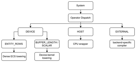
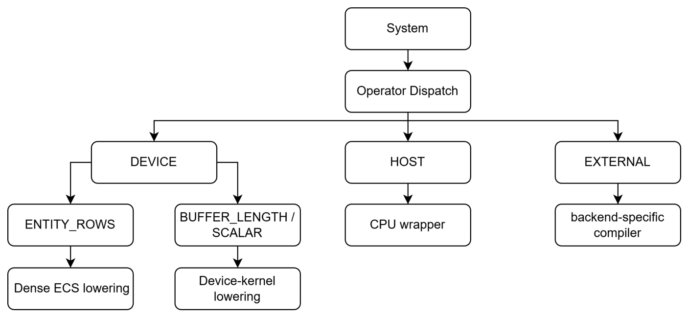
Planning is group-oriented. The planner partitions SystemIR objects by group and processes the groups in authored order. Within each group, it determines the execution domain and dispatches each system according to its operator mode. Figure 2 summarizes this dispatch.

Figure 2. Operator-specific dispatch in the SimDSL planner.

In the default DEVICE path, the planner resolves the system query to the archetypes that satisfy it and emits one dense ECS kernel per matching archetype. DEVICE systems over BUFFER_LENGTH or SCALAR domains are lowered through a separate device-kernel generator that produces backend-owned GPU kernels over dense buffers or scalar control points. HOST systems are translated into CPU-side wrappers that invoke the original Python function with bound world, command-buffer, or resource arguments. EXTERNAL systems are delegated to a backend-registered external compiler.

The planning result is not a symbolic schedule but a group-ordered execution plan. Each group contains a list of callable operations with an execution-domain label indicating whether that group executes on the host or on the device.

For Particle Fountain, emit_particles is specialized to the Emitter archetype, while simulate_particles is specialized to (ParticleLife, ParticleStyle, Position, Velocity). Listing 5 shows the resulting dense ECS representation, where component fields become separate arrays and resource fields are passed as scalar kernel arguments.

Listing 5: Excerpt of emitted dense ECS code for emit_particles. The kernel is specialized to the Emitter archetype: component fields are separate dense arrays, while resource fields are passed as scalar arguments.

extern "C" __global__

void emit_particles(

const int capacity,

const int* live_count,

int* entity_ids,

float* emitter_cooldown,

float* emitter_interval,

float* emitter_vx,

float* emitter_vy,

…

const float dt,

const float gravity,

const float emitter_x,

const float emitter_y,

…

){

int i = blockDim.x * blockIdx.x + threadIdx.x;

if (i < live_count[0]) {

emitter_cooldown[i] = emitter_cooldown[i] + dt;

…

}

}

4.4. Runtime Execution

Runtime execution is implemented by CuPyExecutable. At compilation time, the world state is uploaded into GPU memory by converting archetype entity-id arrays, component columns, dense buffers, and grids into CuPy arrays.

These allocations are served by CuPy’s default device memory pool. Under the fixed-capacity GPU structural path, archetype SoA columns, entity identifiers, live-count counters, and structural command buffers are sized to their declared capacities at upload time. During steady-state execution, staged spawn and destroy update live counts and row contents in place; they do not grow or shrink these arrays, so the pooled footprint for world state remains stable across steps. Reallocation from the pool occurs mainly when CPU-side structural changes trigger world re-upload and plan refresh, not on ordinary per-step GPU-resident structural churn within capacity.

Execution then proceeds step by step through a group-ordered runtime loop. For each simulation step, the runtime first checks whether the structural version of the world still matches the version for which the current plan was compiled. If the structure has changed on the CPU side, the world is re-uploaded, and the plan is rebuilt. The runtime then executes the compiled groups in authored order, invoking each callable associated with the current group.

Device groups launch generated GPU kernels directly. After each group, the runtime applies queued GPU structural commands and flushes any deferred structural commands.

Host groups are integrated into the same execution loop through explicit synchronization. Before a host group executes, the runtime synchronizes the world state back to the CPU, invokes the associated host-side Python operations, and then uploads the modified state again before continuing. Host execution therefore remains part of the compiled runtime model even though the underlying work is performed as Python.

The runtime also provides explicit result extraction. Intermediate state can be inspected through snapshot operations, while complete output is obtained through download. Since these operations are separate from the main execution loop, simulations that remain entirely on the device can keep state GPU-resident throughout the steady-state portion of execution and incur host-device transfer only when explicitly requested.

4.5. Staged Structural Mutation

The staged structural mutation is implemented through deferred command buffers. Structural operations are lowered into writes to device-side command buffers that store command kind, entity identifier, destination archetype, and payload values. After the group completes, a dedicated GPU structural-apply pass consumes these queues and updates archetype rows, live counts, and entity-index mappings. The next group observes the updated structure, while the current group sees a stable structural view of the world.

The emitted code for Particle Fountain makes the staged mutation model explicit. Listing 6 shows how staged entity creation is realized on GPU. The generated kernel does not insert the new entity directly into archetype storage. Instead, it allocates a slot in the GPU structural queue, records the command kind as a spawn, specifies the destination archetype, and packs the new entity’s component values into payload buffers. In this example, the payload includes the emitted particle’s initial position and velocity. The queued command is later consumed by the structural-apply pass, which materializes the actual archetype insertion at the group boundary.

Listing 6: Excerpt of emitted GPU code for staged spawn in emit_particles.

int struct_slot = simdsl_alloc_structural_slot(cmd_count, cmd_overflow);

if (struct_slot >= 0) {

cmd_kind[struct_slot] = STRUCT_SPAWN_KIND;

cmd_entity[struct_slot] = -1;

cmd_dst_arch[struct_slot] = 0;

cmd_payload_f32[(struct_slot*STRUCT_MAX_F32_PAYLOAD)+4] = emitter_x;

cmd_payload_f32[(struct_slot*STRUCT_MAX_F32_PAYLOAD)+5] = emitter_y;

cmd_payload_f32[(struct_slot*STRUCT_MAX_F32_PAYLOAD)+6] = emitter_vx[i];

cmd_payload_f32[(struct_slot*STRUCT_MAX_F32_PAYLOAD)+7] = emitter_vy[i];

}

Listing 7 shows how destroy_entity() is lowered. As in the spawn case, the generated kernel does not immediately rewrite archetype storage. Instead, it allocates a slot in the GPU structural queue, records the command kind as STRUCT_DESTROY_KIND, and stores the identifier of the entity to be removed through cmd_entity. The destination archetype is set to -1, indicating that the operation removes the entity rather than transitioning it into another archetype. The actual removal from archetype storage is deferred until the structural-apply pass executes at the group boundary.

Listing 7: Excerpt of emitted GPU code for staged destroy in simulate_particles.

int struct_slot = simdsl_alloc_structural_slot(cmd_count, cmd_overflow);

if (struct_slot >= 0) {

cmd_kind[struct_slot] = STRUCT_DESTROY_KIND;

cmd_entity[struct_slot] = entity_ids[i];

cmd_dst_arch[struct_slot] = -1;

}

The structural command queue is bounded by a declared capacity. When concurrent device threads enqueue more spawn or destroy requests than this bound allows, additional requests are not recorded and therefore are not applied at the group boundary. The queue is cleared after the structural-apply pass so later groups start from an empty buffer. As with archetype capacity, command capacity is an author-chosen peak bound: It must cover the worst-case structural traffic of a group. Otherwise, excess updates are discarded rather than triggering dynamic reallocation.

5. Optimization

SimDSL does not rely on aggressive whole-program optimization or architecture-specific kernel autotuning. Performance instead comes from a small set of representation-level and lowering-time transformations that turn the authored ECS program into specialized GPU work while preserving staged structural semantics. This section focuses on those transformations and the costs they remove.

5.1. Query-to-Archetype Specialization

At planning time, each ECS query is resolved to the concrete archetypes that satisfy it, and the system is lowered to one dense kernel per matching archetype. This shifts query interpretation out of the hot loop: generated kernels operate directly on that archetype’s SoA columns rather than filtering a heterogeneous entity set at runtime.

5.2. SoA Field Lowering

Component accesses in ECS systems are lowered to indexed loads/stores on per-field dense arrays, with resources passed as scalar kernel arguments. The transformation replaces object-like field access with contiguous columnar traversal, improving locality for archetype-specialized kernels.

5.3. Capacity-Specialized Launch with Live-Count Gating

Under GPU structural mutation, dense kernels are launched over the declared archetype capacity and gated by live_count. This keeps launch geometry stable while restricting useful work to live rows, and avoids reallocating device columns when population changes within capacity.

5.4. Deferred Structural Enqueue

Spawn, destroy, and transition are lowered to atomic enqueues into a device command queue rather than in-place archetype rewrites inside the compute kernel. Compute kernels therefore iterate a stable structural view. Topology updates are confined to the post-group apply pass, which is the performance-relevant consequence of staged mutation.

5.5. Launch-Time State Binding

Resources and buffer/column pointers are bound at kernel launch from the current world state rather than baked into generated code. Per-step scalar updates remain visible without recompilation, while archetype-specialized kernels are retained until a true layout change occurs.

5.6. Selective Plan Reuse

A structural version check reuses the compiled plan across steady-state steps and triggers re-upload/replan only when CPU-side structure changes the effective layout. This avoids repeated compilation and device reallocation in the common GPU-resident case.

5.7. GPU-Resident Steady State

After initial upload, archetype columns, buffers, and grids remain on device for the main loop; host transfers occur for explicit snapshot/download state. Together with fixed-capacity in-place updates, this keeps the CuPy pool footprint for world state stable during ordinary structural churn within capacity.

SimDSL’s performance strategy is specialization and residency: query and layout specialization at planning/lowering time, deferred structural effects at group boundaries, and reuse of compiled GPU-resident plans across steady-state steps—not classical multi-pass kernel optimization.

6. Baseline Implementations

For each workload, we evaluate two matched, straightforward GPU baselines alongside SimDSL: an idiomatic CuPy implementation and a CUDA reference implementation. All three versions use the same workload parameters, step counts, problem sizes, capacities, and initial conditions. The CuPy baselines are written as array-level SoA programs using standard library primitives and do not employ custom fused kernels, shared-memory tiling, or occupancy tuning. The CUDA baselines use straightforward custom global kernels with fixed launch configurations and library sort, compact, or reduction operations where required. They were implemented to reproduce the same simulation behavior as SimDSL, but were not exhaustively tuned or optimized for a particular GPU architecture.

7. Experimental Evaluation

We evaluate SimDSL along four dimensions: support for GPU-resident execution in the steady-state simulation loop, runtime characteristics of the compiled execution model, performance relative to baseline reference implementations, and portability of these results across hardware platforms. Concretely, we ask: (1) whether representative workloads can keep their active simulation state on the GPU without periodic host synchronization or re-upload; (2) how runtime cost is distributed across compiled execution groups and auxiliary runtime overheads; (3) how closely generated SimDSL execution approaches baseline implementations at two levels of manual effort—idiomatic CuPy array programs and hand-written custom CUDA kernels—under identical configurations; and (4) whether these findings hold across both a consumer-class and a server-class GPU.

We evaluate the cross-product of five workloads, two GPU platforms, and three implementations, yielding 30 workload–platform–implementation configurations.

7.1. Experimental Setup and Metrics

We evaluate SimDSL on five representative simulation workloads: Tower Defense, Ant Colony, Particle Fountain, Reaction Diffusion, and Traffic on a Ring Road.

We use these mini-applications because they span the DSL’s target patterns: buffer-domain stencils, fixed-population ECS with shared buffers, high-churn spawn/destroy, agents coupled to evolving fields, and multi-stage hybrid entity buffer loops. These correspond to recurring computational motifs in PDE-style simulation, microscopic traffic, particle/VFX systems, swarm simulation, and discrete games. They serve as representative computational proxies rather than full production applications.

All experiments are conducted under controlled and repeatable conditions: for every workload, all three implementations use identical simulation parameters, identical initial conditions, and the same random seeds where applicable, and each configuration is measured over five independent runs after 10 warm-up steps that exclude JIT compilation and memory-pool initialization from the timed region.

Performance statistics are computed from run-level mean steady-state step times over five independent runs. For the implementation comparison, the primary timing metric is the mean simulation_step_s after excluding the first 10 warm-up steps. If this field is unavailable, the analysis uses simulation_wall_s/timed_steps from the run summary. The frame_total_observed_s field is not used for the implementation comparison because it includes metrics-capture overhead. Throughput is derived from the same timing samples as $\mathrm{FPS}=1000/\mathrm{step}\_\mathrm{ms}$.

For each implementation, we report the mean, standard deviation, and 95% confidence interval over run-level values, with confidence intervals computed using Student’s t-distribution. Pairwise throughput ratios are accompanied by 95% confidence intervals obtained from 10,000 bootstrap resamples over runs. Because the runs are independent rather than paired, differences between implementations are assessed using Welch’s two-sample t-test. Cohen’s d is reported as an effect-size measure. Statistical inference is performed on run-level means rather than individual simulation steps so that repeated steps within a run are not treated as independent observations.

The recorded metrics include per-step simulation time, achieved simulation throughput, profiler-reported per-group execution time, command-flush overhead, host synchronization and upload costs, and memory statistics.

7.1.1. Hardware Configurations

Experiments were conducted on two platforms chosen to span the consumer and server ends of the GPU spectrum:

• Consumer-class platform (RTX 4060): Intel Core i7-12650H, 32GB DDR5-4800 RAM, and an NVIDIA GeForce RTX 4060 Laptop GPU with 8 GB GDDR6 memory, running Windows.
• Server-class platform (H100 NVL): AMD EPYC 9V84 with 40 logical CPUs, 314 GiB RAM, and one NVIDIA H100 NVL GPU with 95830 MiB (≈96 GB) memory, running Ubuntu 24.04.2 LTS with NVIDIA driver 580.105.08 and CUDA 13.0.

7.1.2. Software Configuration

The 4060 platform runs Windows 11; the H100 platform runs Ubuntu 24.04.2 LTS. Both use CuPy 14.0.1 with the cupy-cuda12x build, corresponding to a CUDA 12.x software stack.

Implementations under comparison. Each workload is implemented in three functionally equivalent forms:

• SimDSL: Simulation logic authored in the DSL. The backend lowers authored systems into workload-specialized kernels operating directly over the intended storage layout.
• Baseline CuPy: An idiomatic array-program implementation in which each logical step is expressed as a sequence of library-level array operations (masking, sorting, compaction, scatter/gather, temporary buffer construction). This baseline represents the effort level of a proficient Python/GPU practitioner who does not write custom kernels.
• Baseline CUDA: The CUDA baseline consists of a straightforward CUDA implementation for each workload, launched from a thin Python host loop.

7.1.3. Simulation Configuration

All simulations use fixed parameters across the three implementations (SimDSL, CuPy, CUDA) to ensure fair comparison. Our benchmarks cover dense grid-based updates, large-scale agent systems, and dynamic entity lifecycles. In Particle Fountain, the simulation runs for 8000 steps with a particle capacity of 300,000, 64 emitters, $\mathrm{d}t=0.016$, a horizontal velocity range of $[-6,6]$, a vertical velocity range of $[18,34]$, particle lifetimes in $[1.6,3.2]$, a delay window of $1.0$, and seed 7. In Tower Defense, the benchmark runs for 80,000 steps with 150,000 total enemies, an enemy capacity of 1,000,000, enemy health of $100.0$, enemy speed of $0.7$, a spawn interval of $0.005$, a turret firing interval of $0.01$, turret damage of $1.0$, turret range of 5, and the fixed map demos/map.txt. In Traffic Ring, the simulation runs for 8000 steps with road length 50,000, density $0.85$ (42,500 cars), maximum speed 5, slowdown probability $0.3$, and seed 7. In Reaction Diffusion, the simulation runs for 2000 steps at resolution $256\times 256$, with diffusion rates $D_A=1.0$ and $D_B=0.5$, feed 0.055, kill $0.062$, $\mathrm{d}t=0.016$, and seed size 16. In Ant Colony, the simulation runs for 4000 steps on a $256\times 256$ grid with 50,000 ants, initial food amount 60,000, food/home pheromone deposits $0.60$/$0.25$, evaporation $0.985$, diffusion $0.12$, and seed 7.

7.1.4. Execution Parameters

All SimDSL device kernels are launched using a 1-D thread index i = blockDim.x * blockIdx.x + threadIdx.x. Entity-row systems use a fixed block size of 256 threads and a grid of $\lceil n_{\mathrm{launch}}/256\rceil$, where $n_{\mathrm{launch}}$ is the matched archetype’s fixed capacity (GPU structural mode) or live entity count. Threads guard on i < live_count[0] or i < n.

For buffer-length DEVICE systems (including Reaction Diffusion), the block size is also 256, and the grid is $max(1,\lceil n/256\rceil )$, where n is the length of the extent buffer (for Reaction Diffusion, $n=width\times height$). The stencil is implemented over a linearized index (x = i % w, y = i / w), not a 2-D CUDA launch. Scalar DEVICE systems use a single thread block of size 1.

Deferred structural commands are applied by a dedicated apply_structural kernel launched as $(\mathit{grid},\mathit{block})=(1,1)$.

Component data are stored in dense structure-of-arrays form (one device array per field per archetype).

The CUDA baselines use explicit launch parameters per demo. Entity-oriented kernels (Particle Fountain, Traffic Ring, Tower Defense, and Ant Colony phases) use block size 256 and grid $\lceil count/256\rceil$. Reaction Diffusion in CUDA uses a $16\times 16$ thread block for the update kernel and a 1-D commit kernel with block size 256. These choices are fixed in the reference implementations and were not auto-tuned per device.

A short description of each simulation is given below.

7.1.5. Tower Defense [25]

Enemies spawn at the start of a path and march toward a goal. Towers watch the path, pick nearby enemies as targets, and damage them over time. The simulation ends either when enough enemies escape to the goal or when all spawned enemies have been cleared.

7.1.6. Reaction Diffusion [26]

Two chemicals spread across a 2D field and react with each other over time. Small differences in concentration get amplified by diffusion and reaction, gradually producing spatial patterns. The demo is a dense grid update where every cell evolves based on its neighbors.

7.1.7. Traffic Ring [27]

Cars move around a circular road and repeatedly react to the space in front of them. If the road ahead is clear, they move forward, and if it is blocked, they slow or wait according to the Nagel–Schreckenberg model. Over time, the system shows how local driving rules create collective traffic flow.

7.1.8. Particle Fountain [28]

A set of emitters continuously shoots particles upward like a fountain. Each particle flies through the air, slows and falls because of gravity, and disappears when its lifetime ends or when it hits the floor. The simulation is mostly about repeated creation, motion, and removal of many short-lived entities.

7.1.9. Ant Colony [29]

Many ants move through space while depositing pheromones into the environment. Those pheromone trails influence later movement, producing emergent trail formation and collective behavior. The simulation combines many moving agents with a shared spatial field.

7.2. GPU-Resident Execution

We first evaluate whether SimDSL can sustain GPU-resident execution in the hot loop on both platforms. The relevant criterion is not merely that individual kernels execute on the GPU, but that the active simulation state remains resident on the device across repeated steps without periodic host synchronization or state upload.

Across all five DSL workloads and on both GPUs, the aggregated runtime metrics report host_sync_to_cpu_s = 0 and host_upload_s = 0, indicating that the measured hot loop performs no periodic host-side synchronization or re-upload; measured runtime cost is attributed to device-side execution groups only. Reserved GPU memory remains fixed within each workload configuration, consistent with the preallocated execution model summarized in Table 4.

Table 4. GPU residency evidence per workload. Reserved pool sizes are identical on both platforms; host synchronization and upload time are zero in all configurations.

Simulation	Execution Groups	Reserved Pool
Ant Colony	prepare, ants, cleanup, diffuse, commit	3.15 MiB
Particle Fountain	emit, simulate, structural_apply	14.22 MiB
Tower Defense	spawn, move, attack, cleanup, trace	88.70 MiB
Traffic Ring	prepare, mark, update, trace	1299.4 MiB
Reaction Diffusion	update, commit	1.00 MiB

7.3. Compilation Cost and Complexity

Compilation consists of source inspection and IR construction, query resolution, execution-plan construction, backend lowering, and backend kernel compilation. Let S denote the number of systems, A the number of declared archetypes, N the total size of the captured system ASTs, and $m_i$ the number of archetypes matched by system i.

Source inspection and IR construction parse each system and walk its AST (including access inference), which is linear in the captured program representation, $O(N+S)$. ECS query resolution tests each system query against the declared archetype universe. Treating a signature test as constant-time in the number of components gives $O\left(SA\right)$ query-resolution work; a precise bound is $O\left(SAC\right)$ if C is the signature size. Execution-plan construction then groups systems into ordered groups and is cheap relative to lowering.

DEVICE entity-row ECS lowering emits a specialized kernel for each system–archetype match, so generated code size and lowering work are proportional to ${\sum }_i{m}_i{n}_i$, where $n_i$ is the lowered size of system i. Buffer- or scalar-domain DEVICE systems emit a single kernel. The specialization term therefore applies to the entity-row ECS path. In GPU structural mutation, the backend additionally lowers one structural-apply kernel over the archetype set, which is $O\left(A\right)$ extra codegen independent of S.

Measured compile time is dominated by compilation of these generated device kernels. Modeling that cost as proportional to generated size is a practical summary, not a claim that the vendor compiler is strictly linear. Thus, the compilation cost of the current implementation can be summarized as

$$O\left(N+SA+\sum _i{m}_i{n}_i\right)$$

for entity-row ECS specialization, with the archetype-specialization term becoming most important when many systems match many archetypes. Compilation occurs before steady-state execution, and the resulting execution plan is reused across simulation steps unless structural layout change forces a refresh.

As shown in Table 5, measured end-to-end compilation time ranges from 0.077 s for Reaction Diffusion to 1.884 s for Traffic Ring. Absolute compilation cost, rather than compilation share, provides a direct comparison across workloads. Reaction Diffusion has the lowest compilation cost, followed by Particle Fountain, Tower Defense, and Ant Colony, while Traffic Ring is substantially more expensive to compile. The compilation share depends strongly on simulation duration: it is only 0.32% for Tower Defense, but reaches 24.14% for Reaction Diffusion and 45.79% for Traffic Ring. Because the compiled execution plan is reused across simulation steps, this one-time cost is increasingly amortized as simulation duration grows.

Table 5. End-to-end SimDSL compilation cost on the RTX 4060. Values are mean ± standard deviation over five runs. Compilation share is $\mathrm{compile}/(\mathrm{compile}+\mathrm{simulation}\mathrm{wall})$.

Simulation	Compile (s)	Sim. Wall (s)	Share (%)
Reaction Diffusion	$0.077\pm 0.005$	$0.242\pm 0.027$	24.14
Ant Colony	$0.222\pm 0.034$	$3.201\pm 0.254$	6.49
Particle Fountain	$0.152\pm 0.016$	$2.971\pm 0.326$	4.87
Tower Defense	$0.195\pm 0.015$	$61.643\pm 6.112$	0.32
Traffic Ring	$1.884\pm 0.043$	$2.230\pm 0.149$	45.79

7.4. Comparison with Baseline Implementations

We compare compiled SimDSL with manually implemented CuPy and CUDA reference versions under matched simulation configurations. The comparison evaluates the performance cost or benefit of SimDSL’s generated execution relative to a high-level array-oriented implementation and to a direct CUDA implementation. The CUDA and CuPy implementations should be interpreted as straightforward, manually written reference implementations rather than as an exhaustively hand-tuned upper bound on performance.

Table 6 reports mean steady- state FPS for all 30 configurations. We summarize SimDSL’s position with two normalized quantities: its speedup over CuPy and its efficiency relative to CUDA, where values below 1.0 indicate that the handwritten kernels are faster. The first 10 warm-up steps of each run are excluded from the calculation.

Table 6. Mean steady-state FPS ± standard deviation over five independent runs. FPS is computed from the run-level mean simulation_step_s after excluding the first 10 warm-up steps. Ratios report SimDSL throughput divided by the corresponding baseline throughput.

GPU	Simulation	SimDSL	CuPy	CUDA	vs. CuPy	vs. CUDA
RTX 4060	Ant Colony	1441.8 ± 111.9	163.1 ± 23.1	4899.8 ± 739.3	8.84×	0.29×
	Particle Fountain	3080.3 ± 340.2	364.0 ± 33.9	6339.1 ± 548.6	8.46×	0.49×
	Tower Defense	1386.2 ± 121.3	510.4 ± 179.6	476.3 ± 136.9	2.72×	2.91×
	Traffic Ring	4115.4 ± 283.2	485.4 ± 78.8	2617.2 ± 94.2	8.48×	1.57×
	Reaction Diffusion	11,036.4 ± 1076.3	612.6 ± 79.4	13,002.0 ± 1270.6	18.01×	0.85×
H100 NVL	Ant Colony	5380.8 ± 30.9	434.5 ± 7.0	13,742.6 ± 58.8	12.38×	0.39×
	Particle Fountain	3456.2 ± 9.7	920.0 ± 16.5	12,424.3 ± 109.2	3.76×	0.28×
	Tower Defense	1976.5 ± 6.2	1288.5 ± 674.1	1136.3 ± 2.9	1.53×	1.74×
	Traffic Ring	4744.4 ± 12.3	1772.3 ± 15.2	3067.2 ± 29.1	2.68×	1.55×
	Reaction Diffusion	18,187.4 ± 67.9	1666.9 ± 11.2	40,893.6 ± 388.7	10.91×	0.45×

The primary objective of SimDSL is not to outperform CuPy or CUDA baselines, but to simplify the development of fully GPU-resident simulations that would otherwise require explicit low-level kernel and runtime management. On the RTX 4060, SimDSL outperforms the CuPy reference implementation for all five workloads. The throughput advantage ranges from 2.72× for Tower Defense to 18.01× for Reaction Diffusion. These results indicate that the generated kernels and GPU-resident execution model can substantially reduce the overhead associated with expressing each simulation step as a sequence of high-level array operations. The largest RTX 4060 gain occurs for Reaction Diffusion, where the CuPy version expresses each simulation step through multiple array-level operations and associated runtime orchestration.

Relative to the CUDA reference implementation, the result is workload-dependent. On the RTX 4060, SimDSL outperforms CUDA for Tower Defense and Traffic Ring by 2.91× and 1.57×, respectively. CUDA is faster for Reaction Diffusion, Particle Fountain, and Ant Colony, for which SimDSL achieves 0.85×, 0.49×, and 0.29× of the CUDA throughput, respectively. These results show that SimDSL does not uniformly outperform direct CUDA execution. Its relative performance depends on workload structure and the runtime costs introduced by the compiled execution model.

SimDSL and the CUDA baselines use similar default launch geometry for entity-oriented kernels (256-thread blocks and $\lceil n/256\rceil$ grids), so the observed performance differences cannot be attributed to block size alone. SimDSL incurs additional runtime structure in several workloads: the compiled schedule may be divided into multiple device stages, structural mutations are processed in a separate apply_structural pass, and fixed-capacity archetype kernels may launch over more rows than are currently live. These costs are particularly visible in Particle Fountain and Ant Colony, where the direct CUDA implementations achieve substantially higher throughput.

Tower Defense and Traffic Ring exhibit the opposite result. In these workloads, the generated SimDSL execution achieves higher throughput than the straightforward CUDA references, indicating that the DSL’s specialization, persistent device state, and execution organization can offset its runtime overheads for some workload structures. Reaction Diffusion represents a closer comparison: CUDA is approximately 1.18× faster than SimDSL (the SimDSL/CUDA ratio is 0.85×). The CUDA implementation uses a $16\times 16$ two-dimensional update kernel, whereas SimDSL currently lowers the grid to a one-dimensional launch. The remaining difference is therefore consistent with differences in launch organization and memory-access structure rather than with ECS structural-update overhead, since Reaction Diffusion does not exercise dynamic archetype mutation.

The statistical analysis confirms that the observed differences are generally larger than run-to-run variability. SimDSL achieves significantly higher mean FPS than the CuPy baseline for all five workloads ($p<0.001$). Relative to the CUDA reference implementation, the result remains workload-dependent. SimDSL is significantly faster for Tower Defense and Traffic Ring, whereas CUDA is significantly faster for Reaction Diffusion, Particle Fountain, and Ant Colony. All SimDSL–CUDA bootstrap confidence intervals exclude 1.0.

7.5. Runtime Characteristics

Using the same steady-state simulation_step_s measurements underlying Table 6, the corresponding RTX 4060 SimDSL step times are approximately 0.091 ms for Reaction Diffusion, 0.328 ms for Particle Fountain, 0.726 ms for Tower Defense, 0.244 ms for Traffic Ring, and 0.697 ms for Ant Colony. The first 10 warm-up steps are excluded from these measurements. All five workloads execute with zero measured host synchronization and zero host upload in the original SimDSL configuration.

The H100 NVL reduces the step time for every benchmark. Mean times range from 0.0550 ms for Reaction Diffusion to 0.5060 ms for Tower Defense, with Ant Colony, Traffic Ring, and Particle Fountain requiring 0.1859 ms, 0.2108 ms, and 0.2893 ms, respectively. All workloads therefore sustain interactive execution rates on both platforms.

Runtime resource characteristics for the RTX 4060 are summarized in Table 7. GPU utilization was sampled during the timed simulation region using NVML/nvidia-smi. Mean utilization varies substantially across workloads, from $0.8\%$ for Reaction Diffusion to $34.0\%$ for Tower Defense. Particle Fountain, Traffic Ring, and Ant Colony show mean utilization of $28.9\%$, $21.1\%$, and $12.2\%$, respectively. These values indicate that the evaluated simulations do not continuously saturate the GPU, particularly for short-running or fine-grained workloads. Table 6 and Table 8 use the same RTX 4060 run-level simulation_step_s samples after exclusion of the first 10 warm-up steps. The throughput ratios and statistical comparisons therefore correspond directly to the FPS values reported in the implementation comparison rather than to a separate timing region.

Table 7. Runtime resource characteristics of SimDSL on the RTX 4060. Values are mean ± standard deviation over five runs. CPU RSS denotes host-process resident memory, and GPU pool denotes memory reserved by the CuPy device memory pool.

Simulation	GPU Util. (%)	CPU RSS (MiB)	GPU Pool (MiB)
Reaction Diffusion	$0.8\pm 1.8$	$312.0\pm 0.1$	$1.0\pm 0.0$
Particle Fountain	$28.9\pm 3.2$	$354.3\pm 0.9$	$14.2\pm 0.0$
Tower Defense	$34.0\pm 3.2$	$582.1\pm 0.3$	$88.7\pm 0.0$
Traffic Ring	$21.1\pm 4.1$	$3674.0\pm 0.2$	$1299.4\pm 0.0$
Ant Colony	$12.2\pm 1.6$	$323.8\pm 0.1$	$3.1\pm 0.0$

Table 8. Statistical comparison of run-level mean FPS over five independent runs on the RTX 4060. The ratio denotes SimDSL FPS divided by baseline FPS; values above 1 indicate that SimDSL is faster. Ratio confidence intervals are obtained by bootstrap resampling over runs (10,000 resamples). Welch’s two-sample t-test is used for significance testing, and Cohen’s d is reported as the effect size. Positive d indicates higher mean FPS for SimDSL.

Simulation	Comparison	Throughput Ratio	95% CI	Cohen’s d	Welch p
Reaction Diffusion	SimDSL/CUDA	0.85×	[0.76, 0.94]	−1.67	0.0304
	SimDSL/CuPy	18.01×	[15.79, 20.72]	13.66	<$0.001$
Particle Fountain	SimDSL/CUDA	0.49×	[0.44, 0.54]	−7.14	<$0.001$
	SimDSL/CuPy	8.46×	[7.59, 9.48]	11.24	<$0.001$
Tower Defense	SimDSL/CUDA	2.91×	[2.36, 3.77]	7.03	<$0.001$
	SimDSL/CuPy	2.72×	[2.07, 3.53]	5.71	<$0.001$
Traffic Ring	SimDSL/CUDA	1.57×	[1.48, 1.66]	7.10	<$0.001$
	SimDSL/CuPy	8.48×	[7.41, 9.74]	17.46	<$0.001$
Ant Colony	SimDSL/CUDA	0.29×	[0.26, 0.34]	−6.54	<$0.001$
	SimDSL/CuPy	8.84×	[7.87, 10.16]	15.83	<$0.001$

The GPU memory-pool footprint also varies with workload state size. Reaction Diffusion reserves approximately $1.0$ MiB, Ant Colony $3.1$ MiB, Particle Fountain $14.2$ MiB, Tower Defense $88.7$ MiB, and Traffic Ring $1299.4$ MiB. Host-process resident memory follows the same general workload-size trend, ranging from approximately $312.0$ MiB for Reaction Diffusion to $3674.0$ MiB for Traffic Ring. The GPU pool measure reports memory reserved by CuPy’s device allocator and should not be interpreted as total physical GPU-memory consumption.

7.6. Ablation of Runtime Optimizations

To isolate the contribution of individual runtime mechanisms, we use the SimDSL implementation as the reference configuration and disable one mechanism at a time. The ablations evaluate GPU-resident state, avoidance of per-step host readback, execution-plan reuse, and the CuPy memory pool. Particle Fountain, Reaction Diffusion, and Ant Colony are used because they exercise dynamic ECS execution, dense-grid computation, and mixed agent–field computation, respectively. Each configuration was executed five times.

The ablation experiments use a different timing boundary from the implementation comparison. Specifically, ablation step time is computed as simulation_wall_s/timed_steps so that host synchronization, state upload, plan reconstruction, and other runtime costs introduced by the disabled mechanism remain part of the measured end-to-end step cost. In contrast, Table 6 uses steady-state simulation_step_s. Therefore, absolute SimDSL values from the implementation-comparison and ablation tables should not be compared directly; slowdown ratios within the ablation study are computed using the same timing definition for all modes.

The ablations identify device residency and execution-plan reuse as the dominant runtime optimizations. Table 9 shows that Particle Fountain is the most sensitive workload: disabling plan reuse increases mean step time from 0.371 ms to 88.186 ms (237.42×), while removing residency increases it to 69.571 ms (187.31×). Forced host readback produces a comparable 187.68× slowdown.

Table 9. Ablation of SimDSL runtime mechanisms. Values report mean step time in milliseconds over five runs. Values in parentheses are slowdown relative to the original SimDSL configuration.

Simulation	DSL	No Plan Reuse	No Residency	Host Readback	No Memory Pool
Reaction Diffusion	$0.121\pm 0.012$	$1.335\pm 0.035$	$0.913\pm 0.055$	$0.534\pm 0.036$	$0.119\pm 0.003$
Particle Fountain	$0.371\pm 0.036$	$88.186\pm 14.821$	$69.571\pm 17.051$	$69.710\pm 3.347$	$0.454\pm 0.018$
Ant Colony	$0.800\pm 0.057$	$8.645\pm 0.378$	$5.194\pm 0.126$	$2.447\pm 0.030$	$0.751\pm 0.034$

The same ordering appears for Reaction Diffusion and Ant Colony, with smaller effect magnitudes. Removing plan reuse increases step time by $11.04\times$ and $10.8\times$, respectively. Removing residency increases step time by $7.55\times$ for Reaction Diffusion and $6.49\times$ for Ant Colony, while forced host readback increases it by $4.42\times$ and $3.06\times$.

The measured overhead counters explain much of the residency effect. For Particle Fountain, host synchronization accounts for $98.4\%$ of simulation wall time in the host-readback configuration. When residency is disabled, host synchronization and re-upload together account for approximately $98.95\%$ of wall time. The corresponding non-resident host-transfer fractions are $79.0\%$ for Reaction Diffusion and $81.0\%$ for Ant Colony. Thus, the slowdown is primarily associated with repeated state materialization and transfer rather than with the device kernels themselves.

The memory-pool ablation has a substantially smaller effect than residency or plan reuse. Disabling the CuPy memory pool produces a 1.22× slowdown for Particle Fountain, while the corresponding ratios for Reaction Diffusion and Ant Colony are 0.98× and 0.94×. These results indicate that memory-pool reuse is not a dominant performance factor in the evaluated workloads, although Particle Fountain shows a modest benefit from retaining the pool.

The present experiments therefore do not support a claim that memory-pool reuse materially improves steady-state performance for these workloads, which is consistent with device storage being allocated before the steady-state loop begins. The run-level statistical analysis supports these trends. Disabling plan reuse or GPU residency, or forcing host readback, produces statistically significant slowdowns for Reaction Diffusion, Particle Fountain, and Ant Colony ($p<0.001$), with large effect sizes. The memory-pool effect is substantially smaller: it is statistically significant for Particle Fountain ($p=0.0191$), but not for Reaction Diffusion ($p=0.8566$) or Ant Colony ($p=0.1855$). These results reinforce that residency and execution-plan reuse, rather than allocator pooling, are the dominant runtime mechanisms in the evaluated workloads.

7.7. Limitations

SimDSL was evaluated using a single CuPy/CUDA backend on two NVIDIA platforms: the RTX 4060 and H100 NVL. Portability to other runtimes and hardware architectures remains unverified. Device-side code supports only a restricted subset of Python, and structural mutation is limited to predeclared archetypes with fixed capacities. GPU structural mutation requires fixed per-archetype, entity-index, and command capacities to be declared before execution. The runtime allocates archetype storage and structural metadata to these bounds, and dense map kernels launch over the declared archetype capacity while guarding execution with live_count. These capacities do not grow on the device: spawns are skipped when an archetype is full, structural requests beyond command capacity are not queued, and entity allocation fails when no free IDs remain. The evaluated workloads have known population bounds, but open-ended or highly adaptive simulations would require conservative over-allocation or future support for host-assisted reallocation and plan refresh. The present evaluation also does not include a controlled developer study of programming effort, learning curve, or maintainability. Although SimDSL removes explicit management of kernel launches, device storage, and staged structural command handling from application code, quantifying these software-engineering benefits remains future work. Additionally, the CuPy and CUDA baselines are straightforward reference implementations rather than fully optimized kernels. Therefore, the results do not establish superiority over hand-tuned GPU code.

8. Conclusions

This paper introduced SimDSL, a Python-embedded ECS DSL for GPU-resident simulation. Its compilation pipeline lowers high-level systems and structural operations into archetype-specialized execution plans. Our results show that ECS can function not only as a software organization pattern, but also as a compilation-oriented abstraction for GPU-resident simulation. Experiments on NVIDIA RTX 4060 and H100 NVL GPUs show that SimDSL preserves device residency and achieves favorable performance relative to straightforward CuPy baselines. Comparisons with similarly straightforward CUDA implementations are workload-dependent, indicating that the generated code can approach or exceed direct manual implementations for some workloads but not consistently across all cases. These results should therefore be interpreted as evidence that SimDSL can translate high-level ECS programs into practical GPU execution, rather than as a claim of superiority over hand-optimized CUDA. Additionally, results suggest that high-level ECS modeling and efficient large-scale execution are compatible when supported by staged compilation, archetype-specialized lowering, and runtime support for structural synchronization. Current limitations include restricted device-side Python support, predeclared fixed capacities for structural mutation, and evaluation of a single CuPy/CUDA backend on two NVIDIA GPUs. Moreover, the CuPy and CUDA baselines are straightforward reference implementations rather than exhaustively optimized implementations, so the experiments do not characterize the gap to peak hardware-specific performance. Future work will extend the device-side language fragment, support structural storage growth beyond fixed predeclared capacities, and improve execution of irregular and highly dynamic workloads. We also plan to broaden the backend architecture beyond the current CuPy/CUDA path, evaluate additional hardware platforms, and compare against more heavily optimized GPU implementations. These extensions will help assess the generality of the ECS-based compilation approach across workloads, runtimes, and hardware architectures.

References

- Bernstein, G.L.; Shah, C.; Lemire, C.; DeVito, Z.; Fisher, M.; Levis, P.; Hanrahan, P. Ebb: A DSL for Physical Simulation on CPUs and GPUs. arXiv 2016, arXiv:1506.07577. [Google Scholar] [CrossRef] [Scilit]
- Shacklett, B.; Xie, Z.; Sarkar, B.; Szot, A.; Wijmans, E.; Koltun, V.; Batra, D.; Fatahalian, K. An Extensible, Data-Oriented Architecture for High-Performance, Many-World Simulation. Acm Trans. Graph. 2023, 42, 90. [Google Scholar] [CrossRef] [Scilit]
- Cox, L.; Williams, B.; Vickers, J.; Ward, D.; Headleand, C. Run-time Performance Comparison of Sparse-set and Archetype Entity-Component Systems. In Proceedings of the Computer Graphics and Visual Computing (CGVC); Sheng, Y., Slingsby, A., Eds.; The Eurographics Association: Eindhoven, The Netherlands, 2025. [Google Scholar] [CrossRef]
- Mertens, S. Building an ECS #2: Archetypes and Vectorization|by Sander Mertens|Medium, 2020. Available online: https://ajmmertens.medium.com/building-an-ecs-2-archetypes-and-vectorization-fe21690805f9 (accessed on 9 October 2025).
- Redmond, P.; Castello, J.; Trilla, J.; Kuper, L. Exploring the Theory and Practice of Concurrency in the Entity-Component-System Pattern. arXiv 2025, arXiv:2508.15264. [Google Scholar] [CrossRef] [Scilit]
- Tasnim, A.; Zhao, T. The Essence of Entity Component System. In Proceedings of the 41st ACM/SIGAPP Symposium on Applied Computing (SAC ’26), Thessaloniki, Greece, 23–27 March 2026; pp. 1–10. [Google Scholar] [CrossRef] [Scilit]
- Tasnim, A.; Zhao, T. The Semantics of Entity Component System. SIGAPP Appl. Comput. Rev. 2026, 26, 5–20. [Google Scholar] [CrossRef] [Scilit]
- Makoviychuk, V.; Wawrzyniak, L.; Guo, Y.; Lu, M.; Storey, K.; Macklin, M.; Hoeller, D.; Rudin, N.; Allshire, A.; Handa, A.; et al. Isaac Gym: High Performance GPU-Based Physics Simulation For Robot Learning. arXiv 2021, arXiv:2108.10470. [Google Scholar] [CrossRef] [Scilit]
- Isaac Lab: A GPU-Accelerated Simulation Framework for Multi-Modal Robot Learning. arXiv 2025, arXiv:2511.04831. [CrossRef] [Scilit]
- Catanzaro, B.; Garland, M.; Keutzer, K. Copperhead: Compiling an embedded data parallel language. SIGPLAN Not. 2011, 46, 47–56. [Google Scholar] [CrossRef] [Scilit]
- Rubinsteyn, A.; Hielscher, E.; Weinman, N.; Shasha, D. Parakeet: A just-in-time parallel accelerator for python. In Proceedings of the 4th USENIX Conference on Hot Topics in Parallelism, Berkeley, CA, USA, 6–7 June 2012; HotPar’12. p. 14. [Google Scholar]
- Lam, S.K.; Pitrou, A.; Seibert, S. Numba: A LLVM-based Python JIT compiler. In Proceedings of the Second Workshop on the LLVM Compiler Infrastructure in HPC, New York, NY, USA, 15 November 2015. LLVM ’15. [Google Scholar] [CrossRef] [Scilit]
- Agrawal, A.; Modi, A.N.; Passos, A.; Lavoie, A.; Agarwal, A.; Shankar, A.; Ganichev, I.; Levenberg, J.; Hong, M.; Monga, R.; et al. TensorFlow Eager: A Multi-Stage, Python-Embedded DSL for Machine Learning. arXiv 2019, arXiv:1903.01855. [Google Scholar] [CrossRef] [Scilit]
- Jungmair, M.; Engelke, A.; Giceva, J. HiPy: Extracting High-Level Semantics from Python Code for Data Processing. Proc. ACM Program. Lang. 2024, 8, 736–762. [Google Scholar] [CrossRef] [Scilit]
- Hu, Y.; Li, T.M.; Anderson, L.; Ragan-Kelley, J.; Durand, F. Taichi: A language for high-performance computation on spatially sparse data structures. ACM Trans. Graph. 2019, 38, 1–16. [Google Scholar] [CrossRef] [Scilit]
- Tillet, P.; Kung, H.T.; Cox, D. Triton: An intermediate language and compiler for tiled neural network computations. In Proceedings of the 3rd ACM SIGPLAN International Workshop on Machine Learning and Programming Languages, New York, NY, USA, 22 June 2019; MAPL 2019. pp. 10–19. [Google Scholar] [CrossRef] [Scilit]
- Ragan-Kelley, J.; Barnes, C.; Adams, A.; Paris, S.; Durand, F.; Amarasinghe, S. Halide: A language and compiler for optimizing parallelism, locality, and recomputation in image processing pipelines. SIGPLAN Not. 2013, 48, 519–530. [Google Scholar] [CrossRef] [Scilit]
- Sujeeth, A.K.; Brown, K.J.; Lee, H.; Rompf, T.; Chafi, H.; Odersky, M.; Olukotun, K. Delite: A Compiler Architecture for Performance-Oriented Embedded Domain-Specific Languages. ACM Trans. Embed. Comput. Syst. 2014, 13, 1–25. [Google Scholar] [CrossRef] [Scilit]
- Henriksen, T.; Serup, N.G.W.; Elsman, M.; Henglein, F.; Oancea, C.E. Futhark: Purely functional GPU-programming with nested parallelism and in-place array updates. SIGPLAN Not. 2017, 52, 556–571. [Google Scholar] [CrossRef] [Scilit]
- Ben-Nun, T.; de Fine Licht, J.; Ziogas, A.N.; Schneider, T.; Hoefler, T. Stateful dataflow multigraphs: A data-centric model for performance portability on heterogeneous architectures. In Proceedings of the International Conference for High Performance Computing, Networking, Storage and Analysis, New York, NY, USA, 17–22 November 2019. SC ’19. [Google Scholar] [CrossRef] [Scilit]
- Anderson, C.; Contributors, B. Bevy Engine. 2024. Available online: https://bevyengine.org/ (accessed on 10 April 2025).
- Caini, M. EnTT: Gaming Meets Modern C++. 2024. Available online: https://skypjack.github.io/entt/ (accessed on 11 April 2025).
- Schaller, T. The Specs Book. 2023. Available online: https://amethyst.github.io/specs/docs/tutorials/ (accessed on 12 April 2025).
- Carpay, J. Apecs: A Type-Driven Entity-Component-System Framework. 2018. Available online: https://github.com/jonascarpay/apecs/blob/master/apecs/prepub.pdf (accessed on 13 April 2025).
- Contributors to Wikimedia Projects. Tower Defense-Wikipedia, 2007. Available online: https://en.wikipedia.org/wiki/Tower_defense (accessed on 8 April 2026).
- Contributors to Wikimedia Projects. Reaction–Diffusion System-Wikipedia, 2006. Available online: https://en.wikipedia.org/wiki/Reaction%E2%80%93diffusion_system. (accessed on 8 April 2026).
- Contributors to Wikimedia Projects. Nagel–Schreckenberg Model-Wikipedia, 2010. Available online: https://en.wikipedia.org/wiki/Nagel%E2%80%93Schreckenberg_model (accessed on 8 April 2026).
- Contributors to Wikimedia Projects. Particle System-Wikipedia, 2003. Available online: https://en.wikipedia.org/wiki/Particle_system (accessed on 10 July 2026).
- Contributors to Wikimedia Projects. Ant Colony-Wikipedia, 2004. Available online: https://en.wikipedia.org/wiki/Ant_colony (accessed on 8 April 2026).
Disclaimer/Publisher’s Note: The statements, opinions and data contained in all publications are solely those of the individual author(s) and contributor(s) and not of MDPI and/or the editor(s). MDPI and/or the editor(s) disclaim responsibility for any injury to people or property resulting from any ideas, methods, instructions or products referred to in the content. |
© 2026 by the authors. Licensee MDPI, Basel, Switzerland. This article is an open access article distributed under the terms and conditions of the Creative Commons Attribution (CC BY) license.