


Abstract
Accurate pole–zero determination is essential for predicting the frequency response, stability, and bandwidth of analog circuits. Conventional transfer function derivations based on nodal or mesh analysis, however, often produce lengthy symbolic expressions and provide limited physical insight, particularly for high-order networks. This paper presents a generalized order-reduction method for deriving the transfer functions of linear time-invariant analog circuits with constant coefficients. The proposed approach decomposes a higher-order network into lower-order configurations and determines the coefficients of its characteristic and zero polynomials by selectively suppressing or isolating energy storage elements. First-order time constants are obtained from the equivalent resistance or conductance associated with each capacitor or inductor. Higher-order coefficients are then evaluated by systematically considering combinations of energy storage elements and successively reducing the network order. The relationship between driving-point impedance and admittance is also employed to establish a unified procedure for determining poles and zeros. The method is applicable to passive and active RLC circuits, including networks containing dependent sources and transistor small-signal models. Several representative examples, ranging from elementary RC networks to higher-order active circuits, are analyzed to demonstrate the derivation procedure and its ability to retain explicit dependence on circuit parameters. Compared with direct symbolic expansion, the proposed framework reduces algebraic manipulation while preserving the physical interpretation of the resulting coefficients. The method therefore provides a systematic and design-oriented tool for transfer function characterization and pole–zero analysis of linear analog circuits.
1. Introduction
The analysis of analog circuits is a fundamental step in predicting their frequency-domain behavior and guiding design optimization. In particular, an accurate transfer function provides essential information about circuit gain, bandwidth, stability, transient response, and sensitivity to component variations. Although the transfer function of a linear time-invariant (LTI) circuit can, in principle, be obtained using conventional nodal or mesh analysis, the resulting algebraic expressions often become prohibitively complex as the number of energy storage elements increases. This complexity is even more pronounced in active circuits containing dependent sources and transistor small-signal models. Consequently, systematic methods that simplify the determination of transfer function coefficients while preserving their physical relationship with circuit parameters are highly desirable.
Early developments in network analysis established the theoretical basis for interpreting the frequency and transient responses of linear circuits. Bode introduced a systematic framework for network analysis and feedback amplifier design [1]. Elmore subsequently investigated the transient response of damped linear networks, with particular emphasis on wideband amplifiers [2]. The influence of pole and zero locations on the transient response of linear dynamic systems was then studied by Mulligan [3]. These foundational contributions demonstrated that circuit equations derived using conventional mesh or nodal analysis could be represented and solved through linear algebraic formulations. Although such formulations are well suited to numerical implementation, they do not always provide the explicit relationships between individual circuit elements and the resulting poles and zeros that are needed for design-oriented analysis. Related classical studies established additional foundations for circuit and polynomial analysis but generally relied on approximate results or algebraically intensive derivations [4,5].
Subsequent research focused on improving the accuracy and applicability of network-analysis techniques [6,7,8]. Among these developments, the open-circuit time constant (OCTC) method emerged as an important approach for estimating the high-frequency behavior of transistor circuits [7]. The principles underlying this method were also considered in the systematic determination of electronic circuit transfer functions [8]. The zero-value time constant (ZVTC) method was later introduced to facilitate the analysis of network responses and transfer function coefficients [9,10,11]. In contrast to methods primarily concerned with denominator coefficients and pole estimation, the ZVTC framework also provided a basis for investigating the contribution of zeros to the transfer function numerator.
Time constant-based analysis was subsequently extended to resistor–capacitor networks and transistor-level analog circuits. Signal-delay analysis in RC-tree networks provided further insight into the relationship between circuit topology and dynamic response [12]. The application and categorization of time constant methods for MOS transistor circuits were also discussed in the context of analog integrated-circuit analysis and design [13]. These methods have become valuable tools because they relate circuit elements directly to the dominant dynamic characteristics of a system. Nevertheless, their use is often limited to approximate pole estimation or to particular circuit structures.
A systematic representation of characteristic-polynomial coefficients in terms of circuit time constants was presented by Rosenstark [14]. Middlebrook later introduced the extra-element theorem as a powerful means of determining the effect of an additional circuit element on a network transfer function [15]. The OCTC method was also extended to networks containing transcapacitances, thereby improving its applicability to active circuits and transistor small-signal models [16]. Further studies examined the use of OCTC and short-circuit time constant (SCTC) techniques for estimating the upper and lower cutoff frequencies of linear circuits and for establishing relationships between circuit topology and bandwidth [17,18,19].
Additional systematic methods were subsequently developed for determining the characteristic and zero polynomials of electronic circuits. In particular, two related approaches were reported for evaluating transfer function coefficients and accounting for multiple circuit elements [20,21]. The Cochrun–Grabel method was later extended to circuits containing mutual inductances [22]. These developments substantially expanded the scope of time constant and element-based circuit analysis. However, when applied to higher-order circuits, they may still require extensive symbolic manipulation and the evaluation of numerous intermediate networks. Therefore, the efficient extraction of poles and zeros from complex active and passive circuits remains an important analytical problem.
The relevance of SCTC and OCTC methods to circuit analysis and design was revisited by Salvatori and Conte, who demonstrated their educational and practical value in estimating frequency-response characteristics [23]. A generalized time- and transfer-constant framework was subsequently introduced by Hajimiri to determine the coefficients of circuit transfer functions systematically [24]. This framework represented a significant advance because it unified several conventional time constant concepts and provided a general formulation for evaluating transfer function coefficients. Nevertheless, the calculation of higher-order coefficients can remain cumbersome, particularly when many energy storage elements and dependent sources are present.
To reduce this computational burden, the authors previously proposed an order-reduction method for determining the characteristic function of LTI analog circuits [25]. The method evaluates denominator coefficients by decomposing a higher-order circuit into lower-order networks and selectively suppressing individual energy storage elements. This decomposition establishes direct relationships between the circuit components, the associated time constants, and the characteristic-polynomial coefficients. However, the previous formulation primarily addressed the denominator of the transfer function and, consequently, the determination of circuit poles.
Efficient transfer function analysis is particularly important in CMOS–MEMS systems, where the coupled dynamics of the sensing element and readout circuitry determine bandwidth, stability, sensitivity, and noise performance. A recent CMOS-integrated micro search-coil magnetometer combining an on-chip sensor with a low-noise instrumentation amplifier exemplifies the need for systematic, design-oriented analysis of such integrated systems [26,27].
More recently, approximate symbolic pole/zero expressions valid near a specified design point have been obtained from a symbolic state (or “state-like”) matrix through open-/short-circuit element replacement, matrix-order reduction, and LR iterations [28]. Similarly, an ensemble heuristic–metaheuristic approach combining root splitting with simulated annealing has been proposed to simplify symbolic pole/zero expressions of operational transconductance amplifiers, implemented in MATLAB R2024b [29].
The present work extends the order-reduction concept to the systematic calculation of transfer function zeros. The proposed method treats pole and zero extraction within a common analytical framework. The characteristic polynomial is obtained by evaluating the natural response of the circuit, whereas the zero polynomial is determined by examining the corresponding input–output behavior and appropriate driving-point functions. By exploiting the reciprocal relationship between driving-point impedance and admittance, zeros of one function can be interpreted as poles of the reciprocal function. The coefficients of the resulting polynomial are then determined by isolating individual energy storage elements, analyzing their pairwise and higher-order combinations, and successively reducing the network order.
The principal contributions of this work can be summarized as follows:
- Extension of the order-reduction method to zero-polynomial analysis: The previously developed approach for characteristic-function evaluation is generalized to determine transfer function zeros.
- Unified treatment of poles and zeros: Pole and zero extraction are formulated using related reduced-order networks, equivalent resistances or conductances, and time constants.
- Systematic calculation of higher-order coefficients: The coefficients associated with combinations of capacitors and inductors are obtained through successive network-order reduction rather than direct symbolic expansion.
- Applicability to general linear analog circuits: The proposed procedure can be applied to passive and active RLC networks, including circuits containing dependent sources and transistor small-signal models.
- Preservation of design insight: Because the resulting coefficients remain explicitly expressed in terms of circuit elements, the effect of parameter variations on pole and zero locations can be identified directly.
The proposed method is intended to complement, rather than replace, conventional nodal, mesh, and symbolic circuit analysis techniques. Its main advantage is that it avoids the complete expansion of large systems of equations when only the transfer function coefficients or pole–zero locations are required. It therefore offers a physically interpretable and design-oriented approach to the analysis of higher-order analog circuits.
The remainder of this paper is organized as follows: Section 2 reviews the frequency response of LTI circuits and discusses the effects of poles and zeros on transfer function magnitude. Section 3 presents the derivation of characteristic equations for different circuit configurations and summarizes the order-reduction procedure for pole calculation. Section 4 extends the proposed framework to zero analysis and demonstrates its application to representative higher-order networks. Finally, Section 5 presents the main conclusions of the study.
2. The Frequency Response
2.1. General Considerations
Frequency-response analysis is one of the principal methods used to characterize the behavior of an analog electronic system. For a linear time-invariant (LTI) circuit, the frequency response describes the variation in the magnitude and phase of the output signal as a function of the input-signal frequency. Because important performance parameters—including gain, bandwidth, phase margin, and attenuation—depend on frequency, frequency-response analysis provides essential information for both circuit evaluation and design optimization.
In analog circuits without explicit inductors, the frequency-dependent behavior is primarily determined by resistive elements and energy storage elements such as intrinsic, parasitic, and externally connected capacitors. More generally, the dynamic behavior of an RLC circuit is governed by the interaction among its resistors, capacitors, inductors, and controlled sources. This behavior can be represented using a transfer function, defined as the ratio of a selected output variable to an input excitation in the Laplace domain. A general factored representation of the transfer function is
where Adc0 denotes the low-frequency or DC gain, z1, z2, …, zm denote the zero parameters, and p1, p2, …, pn denote the pole parameters. With the sign convention adopted in (1), the corresponding roots are located at s = −zi and s = −pi, respectively. Depending on the circuit topology, these roots may be real or complex and may lie in either the left- or right-half of the complex s-plane. As far as the proposed procedure yields the exact polynomial coefficients rather than a pre-factored, root-separated expression, the resulting characteristic and zero polynomials may in general have real, complex-conjugate, or repeated (multiple-order) roots; the proposed derivation applies identically regardless of how these roots are distributed.
An equivalent polynomial representation of the transfer function is as follows:
where a0, a1, …, am and b1, b2, …, bn are constant coefficients determined by the circuit elements and topology. For a normalized numerator, a0 may be set to unity, with the constant scaling incorporated into Adc0. The denominator polynomial in (2) is commonly referred to as the characteristic polynomial or characteristic equation when it is equated to zero. Its roots determine the natural modes and poles of the circuit. Similarly, the roots of the numerator polynomial determine the transfer function zeros.
Consequently, complete characterization of a rational transfer function requires determination of its gain, poles, and zeros. A zero corresponds to a value of s for which the numerator vanishes, whereas a pole corresponds to a value of s for which the denominator vanishes. On the frequency axis, poles and zeros alter the slope and phase of the frequency response. For example, an isolated real zero introduces an asymptotic magnitude slope of +20 dB/decade beyond its break frequency, whereas an isolated real pole introduces a slope of −20 dB/decade.
Before calculating the exact transfer function, it is often useful to determine whether a particular energy storage element contributes a pole, a zero, or a pole–zero pair. Although conventional nodal and mesh analyses can provide exact results, their direct application to higher-order circuits frequently produces lengthy symbolic expressions. A topology-based interpretation of the behavior associated with each energy storage element can therefore provide useful physical insight and simplify the subsequent calculation.
Since the phase response follows directly once the poles, zeros, and DC gain are known, the discussion in this paper emphasizes the magnitude response and the underlying pole–zero locations.
2.2. Poles and Zeros
The poles and zeros of a transfer function play complementary roles in shaping the magnitude and phase responses of an analog circuit. In a conventional Bode-magnitude representation, a pole causes the response slope to decrease, whereas a zero causes it to increase. The net frequency response is determined by the order in which these break frequencies occur and by the cumulative contributions of all poles and zeros.
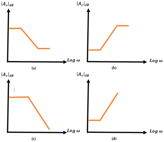
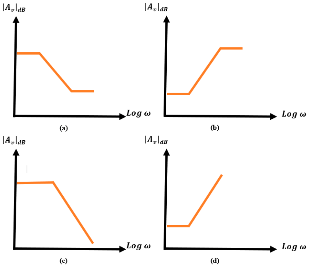
As illustrated conceptually in Figure 1, four elementary magnitude-response patterns can be identified:
Figure 1.
Representative Bode-magnitude responses associated with four elementary pole–zero arrangements: (a) a pole followed by a zero; (b) a zero followed by a pole; (c) a single pole; and (d) a single zero.
- (a)
- A pole followed by a zero;
- (b)
- A zero followed by a pole;
- (c)
- A single pole;
- (d)
- A single zero.
These elementary patterns provide a convenient basis for interpreting the role of individual energy storage elements in more complicated circuits.
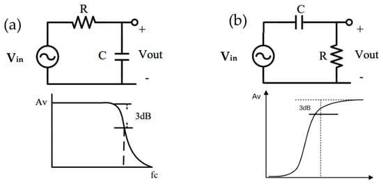
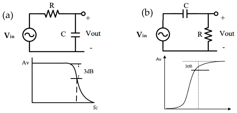
To illustrate this interpretation, consider the first-order low-pass RC circuit shown in Figure 2a. The transfer function is defined as the ratio of the output voltage to the input voltage. At sufficiently low frequencies, the capacitor behaves approximately as an open circuit, and no current flows through the resistor. Therefore, the output voltage approaches the input voltage, and the low-frequency gain approaches unity.
Figure 2.
First-order (a) RC low-pass circuit and (b) RC high-pass circuit used to demonstrate the magnitude-response contribution of an isolated pole.
The capacitor impedance is given by ZC = 1/(sC), or ZC = 1/(jωC) under sinusoidal steady-state conditions. As the frequency increases, the magnitude of the capacitor impedance decreases. Applying the voltage-divider relation gives
Substituting ZC = 1/(sC) into (3) produces the familiar first-order low-pass transfer function H(s) = 1/(1 + sRC). Thus, the circuit contains a single pole at s = −1/(RC). As the excitation frequency exceeds the corresponding pole frequency, the magnitude decreases with an asymptotic slope of −20 dB/decade.
The elementary cases illustrated in Figure 1 may be described more precisely as follows:
- A pole followed by a zero:As the frequency increases beyond the pole frequency, the magnitude begins to decrease. When the zero frequency is reached, the zero contributes an opposing positive slope. If both roots are first order, the net high-frequency slope returns to its original value, as illustrated in Figure 1a.
- A zero followed by a pole:The magnitude initially increases after the zero frequency is crossed. At the subsequent pole frequency, the negative slope introduced by the pole compensates for the positive slope introduced by the zero. This behavior is illustrated in Figure 1b.
- A single pole:The magnitude decreases beyond the pole frequency and continues to decrease in the absence of a compensating zero, as shown in Figure 1c.
- A single zero:The magnitude increases beyond the zero frequency and continues to increase in the absence of a compensating pole, as shown in Figure 1d.
To apply this qualitative interpretation to a higher-order network, the circuit can be decomposed into lower-order configurations. For a selected energy storage element, the remaining storage elements are temporarily suppressed according to their zero-valued representations. A zero-valued capacitor is replaced by an open circuit because its admittance sC becomes zero, whereas a zero-valued inductor is replaced by a short circuit because its impedance sL becomes zero. The resulting first-order network can then be examined to determine whether the selected element produces an isolated pole, an isolated zero, or a pole–zero pair. Repeating this procedure for the remaining storage elements provides an initial topology-based interpretation of the complete response.
As a second example, consider the first-order high-pass RC circuit shown in Figure 2b. At zero frequency, the capacitor behaves as an open circuit and prevents the input signal from reaching the output node. Accordingly, the output voltage is zero, indicating the presence of a zero at the origin.
As the frequency increases, the magnitude of the capacitor impedance decreases, and a larger fraction of the input voltage appears across the resistor. Consequently, the magnitude of the voltage transfer function increases. At sufficiently high frequencies, the capacitor approaches a short-circuit condition and the output voltage approaches the input voltage. The gain therefore converges to unity rather than increasing indefinitely. This transition corresponds to a zero followed by a pole, consistent with the response illustrated in Figure 1b.
The high-pass transfer function can be written as Equation (4) which explicitly contains a zero at s = 0 and a pole at s = −1/(RC).
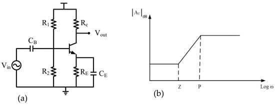
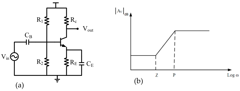
As a final example, consider the common-emitter amplifier with an emitter resistor and bypass capacitor shown in Figure 3a. Neglecting secondary effects, the magnitude of its voltage transfer function can be approximated by
where RC is the effective collector resistance, gm is the transistor transconductance, and ZE is the frequency-dependent impedance connected to the emitter. At low frequencies, the bypass capacitor behaves as an open circuit, and the emitter impedance includes the degeneration resistance RE. The low-frequency gain magnitude is therefore approximately
Figure 3.
Common-emitter amplifier with emitter degeneration and capacitive bypassing: (a) circuit configuration and (b) qualitative Bode-magnitude response showing the zero–pole pair introduced by the emitter-bypass network.
As the frequency increases, the impedance of the bypass capacitor decreases, progressively reducing the effective emitter impedance. The magnitude of the voltage gain therefore increases, indicating the contribution of a zero. At sufficiently high frequencies, the bypass capacitor effectively short-circuits RE, and the gain approaches the approximately constant value gmRC. The termination of the increasing magnitude slope indicates the presence of a pole following the zero. The corresponding qualitative Bode-magnitude response is shown in Figure 3b.
These examples demonstrate that the frequency-dependent contribution of an energy storage element can often be interpreted by isolating its associated first-order subnetwork. The central concept of the proposed approach is therefore to decompose a higher-order circuit into a set of reduced-order networks whose individual pole and zero contributions can be determined more directly. The order-reduction procedure previously applied to pole calculation is summarized in the following section and subsequently extended to the systematic determination of transfer function zeros.
3. Characteristic Equations of Different Configurations
3.1. Pole Analysis
Several methods have been developed for calculating the poles of linear analog circuits. As discussed in the preceding sections, many conventional approaches require extensive algebraic manipulation, particularly when applied to higher-order networks. Moreover, approximate methods may lose accuracy when the circuit poles are not sufficiently separated. The objective of the present method is to determine the characteristic polynomial through systematic network-order reduction, thereby avoiding the direct expansion of large nodal or mesh-equation systems.
To introduce the procedure, consider again the first-order RC low-pass circuit shown in Figure 2. The characteristic equation is obtained by setting the denominator of the transfer function equal to zero. For a first-order network, it can be expressed in the general form
where A has the dimension of time and represents the time constant associated with the single energy storage element. For the circuit in Figure 2, the resistance observed from the capacitor terminals is R, and the corresponding time constant is RC. Equation (7) therefore becomes
1 + As = 0
1 + RCs = 0
The circuit consequently has a pole at s = −1/(RC).
For a second-order network, the characteristic equation can be written as
where A has the dimension of time and B has the dimension of time squared. Such a circuit contains two independent energy storage elements. For an RC network, the coefficient A can be calculated as the sum of the first-order time constants associated with the individual capacitors, with all other capacitors replaced by their zero-valued equivalents. The higher-order coefficient B can then be determined by reducing the circuit order.
1 + As + Bs2 = 0,
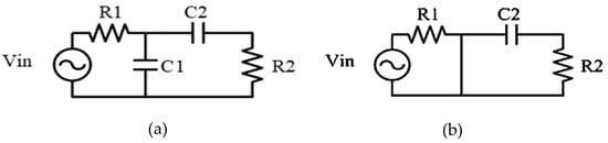
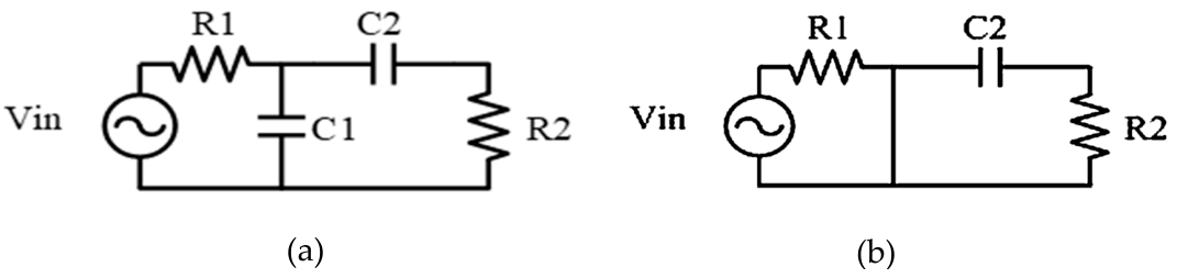
Consider the second-order RC network shown in Figure 4a. The two energy storage elements are C1 and C2.
Figure 4.
(a) Representative second-order RC network and (b) Reduced first-order equivalent of the circuit, obtained in the limit C1 → ∞.
Following the time constant principle associated with Elmore’s analysis [2], the first-order coefficient is obtained by summing the individual time constants:
A = R1C1 + (R1 + R2)C2.
The characteristic equation therefore becomes
1 + [R1C1 + (R1 + R2)C2]s + Bs2 = 0.
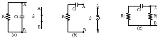
To determine B, the circuit order must be reduced from two to one while preserving the time constant associated with the remaining energy storage element. Depending on the topology, this reduction can be achieved by forcing an appropriate resistance or capacitance toward zero or infinity. For the circuit in Figure 5, two possible operations are:
Figure 5.
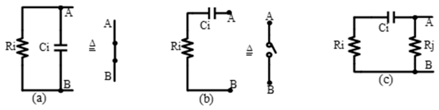
Elementary RC configurations used in the network-decomposition procedure: (a) parallel RC branch, (b) series RC branch, and (c) combined series–parallel configuration.
- Allowing R2 to approach infinity; or
- Allowing C1 to approach infinity.
Using the second operation transforms the original circuit into the reduced first-order network shown in Figure 4b. The characteristic equation of the reduced circuit is
1 + R2C2s = 0.
To relate the reduced-order equation to the original second-order polynomial, divide the left-hand side of (11) by C1 and evaluate the limit C1 → ∞:
The resulting expression must be proportional to the characteristic equation in (12). Multiplication of (12) by R1s gives
from which the second-order coefficient is obtained as
R1s + R1R2C2s2 = 0,
B = R1R2C1C2.
Consequently, the complete characteristic equation of the circuit in Figure 4b is
1 + [R1C1 + (R1 + R2)C2]s + R1R2C1C2s2 = 0.
The same principle can be generalized to an nth-order circuit. For a normalized characteristic polynomial,
the first-order coefficient of an RC network is
where denotes the equivalent resistance observed from the terminals of Ci. When calculating , all independent sources are deactivated, and all other capacitors are assigned their zero values. Accordingly, independent voltage sources are short-circuited, independent current sources are open-circuited, and dependent sources remain active.
1 + As + Bs2 + Cs3+ ⋯ = 0.
The coefficient A is equivalent to the first-order coefficient obtained using the generalized time- and transfer-constant formulation in [24]. This equivalence can also be verified dimensionally. Because every term in a characteristic equation must be dimensionless and s has units of inverse time, the coefficient multiplying s must have units of time. Similarly, B, C, and the subsequent coefficients must have units of time squared, time cubed, and so forth.
The higher-order coefficients are determined through successive order reduction. For example, the second-order characteristic equation
can be reduced to a first-order equation by dividing it by a suitable component value and forcing that component toward zero or infinity. The selected operation must preserve the relevant time constant of the remaining reduced network. The coefficient of s2 in the original equation then contributes to the coefficient of s in the reduced-order equation.
1 + As + Bs2 = 0,
As described in [25], the original network can be decomposed into the three elementary RC configurations shown in Figure 5:
- Parallel RC configuration: The resistance associated with the capacitor is first calculated, after which the corresponding branch is replaced by a short circuit for the subsequent reduction step.
- Series RC configuration: The equivalent resistance is calculated, after which the corresponding branch is replaced by an open circuit.
- Combined series–parallel configuration: The network is analyzed in two stages. First, one equivalent resistance is evaluated while the associated branch is treated as an open circuit. The second resistance is then evaluated after the first resistance is set to zero and the corresponding branch is treated as a short circuit.
Using these reduced configurations, the second-order coefficient for a circuit containing multiple capacitors can be expressed as a sum of pairwise contributions:
where Rb,ij denotes the equivalent resistance associated with capacitor Ci when only Ci and Cj are retained in the reduced network. Similarly, Rb,ji is the equivalent resistance associated with Cj after the reduction operation involving Ci has been applied. All capacitors other than the selected pair are assigned zero values.
The third-order coefficient is obtained by considering all combinations of three energy storage elements:
Here, the resistance factors represent the sequentially evaluated equivalent resistances associated with each selected triplet. All energy storage elements outside the selected triplet are assigned zero values. The same procedure can be extended to fourth- and higher-order coefficients by considering the corresponding higher-order combinations.
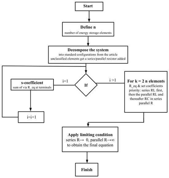
Figure 6 shows a flowchart of the generalized order-reduction procedure, the network is decomposed into standard sub-configurations; the first-order coefficient is obtained by summing the individual time constants of each energy storage element; each higher-order coefficient is then obtained by evaluating the equivalent resistance of increasing element combinations (series RL, parallel RL, then series RC) and applying the limiting conditions (series R → 0, parallel R → ∞). This generalized order-reduction procedure is subsequently applied to the systematic determination of both the characteristic-polynomial coefficients and the zero-polynomial coefficients.
Figure 6.
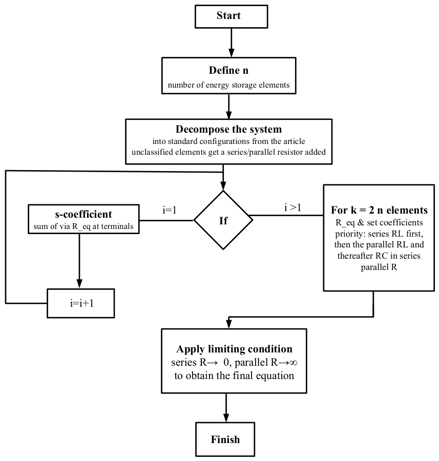
A flowchart describing the proposed method.
When a capacitor is selected as the element whose value approaches infinity, the equivalent resistance of the original network must remain consistent with that of the resulting reduced-order circuit. Each energy storage element should therefore be classified according to one of the elementary configurations in Figure 5. If an element cannot be represented directly by any of these configurations, an auxiliary element may be introduced to facilitate the decomposition. After completing the analysis, the auxiliary element is assigned a limiting value of zero or infinity so that it does not change the order or behavior of the original circuit [25].
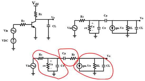
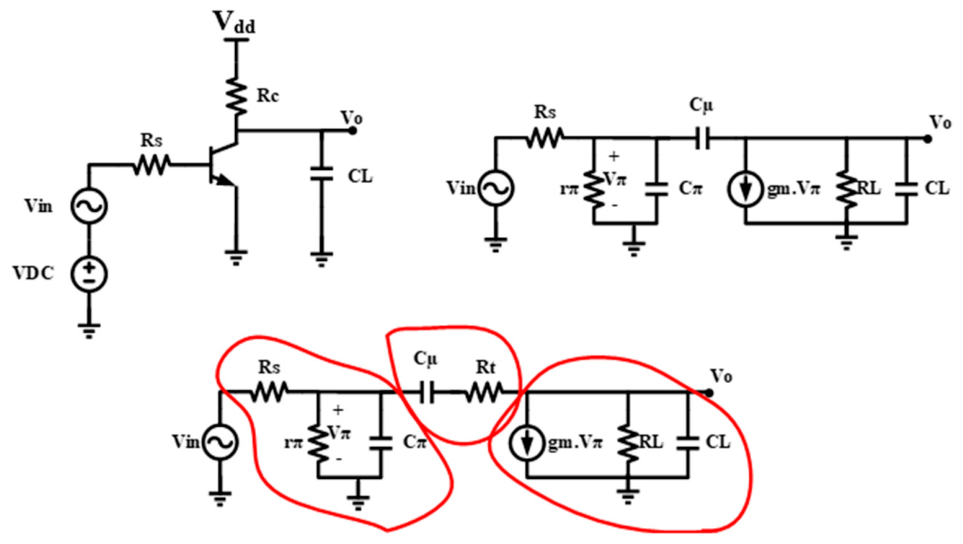
To illustrate this treatment, consider the common-emitter amplifier and its small-signal equivalent circuit shown in Figure 7. The circuit includes the base–emitter capacitance Cπ, the base–collector capacitance Cμ, the load capacitance CL, and the dependent current source gmVπ.
Figure 7.
Common-emitter amplifier used to demonstrate the decomposition of an active circuit containing dependent sources: original circuit, small-signal equivalent model, and modified model incorporating the auxiliary resistance Rt.
In the small-signal model, Cμ connects the input and output nodes and cannot be classified directly as a simple series or parallel RC branch. An auxiliary resistance Rt is therefore introduced in the Cμ branch to enable systematic decomposition. After deriving the characteristic polynomial, the limit Rt → 0 is applied to recover the original circuit.
Defining the effective output resistance as
the characteristic equation of the modified network can be written as
RL = RC‖ro,
Because the three capacitors form a capacitive loop when Rt = 0, they do not provide three independent state variables. Accordingly, the cubic coefficient vanishes in the original circuit. Applying Rt → 0 to (24) gives
This result demonstrates that the apparent number of capacitors does not necessarily equal the dynamic order of a circuit. Capacitive loops and inductive cutsets can reduce the number of independent state variables and, consequently, the degree of the characteristic polynomial.
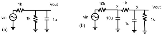
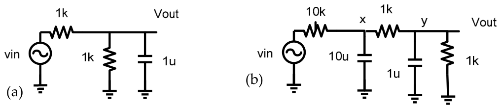
For a first-order network, the pole is obtained directly as the negative reciprocal of the corresponding time constant. For example, the circuit in Figure 8a has a pole
Figure 8.
(a) Representative first-order circuit used to demonstrate direct pole calculation from the equivalent time constant. (b) Representative second-order circuit with well-separated time constants used to illustrate approximate individual pole estimation.
For a higher-order network, approximate pole locations may be estimated by treating the system as a collection of first-order subnetworks. This approximation is reliable when the poles are sufficiently separated, meaning that the individual time constants differ by a substantial margin. Under this condition, the largest time constant determines the dominant pole, while the smaller time constants correspond approximately to the higher-frequency poles.
For the second-order network shown in Figure 8b, the first approximate pole is
whereas the second approximate pole is
Because the two pole frequencies are separated by more than one decade, the individual first-order approximations provide a useful interpretation of the overall response. If the poles are closely spaced, however, the roots should instead be calculated from the complete characteristic polynomial.
3.2. Zero Analysis Using Driving-Point Functions
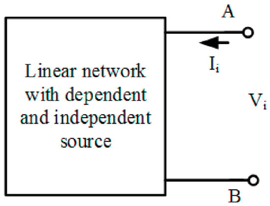
The order-reduction procedure can be extended to transfer function zeros by examining the driving-point functions of the circuit. Consider the general linear network shown in Figure 9. Its driving-point impedance and admittance are defined as
Figure 9.
General linear network used to define the driving-point impedance and admittance at the input port. A, B is the input port for the linear network.
Using the conventional determinant representation of a linear network, the input impedance may be written as
where N11(s) and D11(s) denote the numerator and denominator polynomials associated with the selected driving point. The corresponding input admittance is
Equations (29) and (30) show that the poles of the impedance are the zeros of the admittance, while the zeros of the impedance are the poles of the admittance. This reciprocal relationship provides a systematic mechanism for converting zero determination into a pole-calculation problem.
The required polynomials can be obtained by applying two different input excitations. First, the input is driven by an ideal voltage source. To determine the corresponding natural-response polynomial, the voltage source is set to zero and replaced by a short circuit. Second, the input is driven by an ideal current source. Setting this source to zero produces an open circuit at the input. The characteristic equations of these two modified networks provide the denominator and numerator polynomials of the driving-point function.
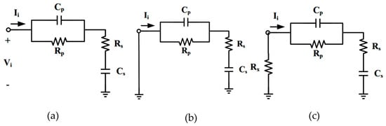
Consider the circuit shown in Figure 10a, which consists of a parallel RC subnetwork cascaded with a series RC subnetwork. Figure 10b shows the circuit obtained when the input voltage source is deactivated, whereas Figure 10c represents the circuit with the current source deactivated.
Figure 10.
Driving-point network used to demonstrate zero extraction: (a) original circuit, (b) network obtained by deactivating the input voltage source, and (c) network obtained by deactivating the input current source and introducing the auxiliary resistance Rx.
When the voltage source is set to zero, it is replaced by a short circuit, as shown in Figure 10b. Applying the pole-calculation procedure to this network gives
1 + [R1C1 + (R1 + R2)C2]s + R1R2C1C2s2 = 0.
For the second case, an ideal current source is applied at the input. When the current source is deactivated, the input becomes open-circuited. To represent this condition algebraically, an auxiliary resistance Rx is connected at the input and subsequently allowed to approach infinity. Before applying the limit, the characteristic equation of the modified circuit is
Dividing (33) by Rx and evaluating the limit Rx → ∞ yields
C2s + R1C1C2s2 = 0.
The input impedance can therefore be expressed as
and the corresponding input admittance is
The numerator and denominator in (29) exchange their roles in (36). Accordingly, the zeros of Zi(s) are the poles of Yi(s), and the poles of Zi(s) are the zeros of Yi(s). This observation forms the basis of the generalized zero-calculation procedure developed in the following section. By deriving the appropriate reduced-network characteristic equations, transfer function zeros can be determined using the same order-reduction principles applied to pole calculation.
The presented derivations were carried out by hand; for high-order polynomials, software such as MATLAB may be used to numerically determine the corresponding poles and zeros.
4. Generalized Method for Zero Analysis
4.1. Systematic Determination of the Zero Polynomial
The order-reduction procedure introduced for pole calculation can also be extended to the systematic determination of transfer function zeros. As discussed in Section 3.2, the zeros of a transfer function are the roots of its numerator polynomial. Therefore, the proposed procedure constructs the zero polynomial directly by analyzing reduced-order versions of the original circuit.
Similar to the calculation of the characteristic polynomial, the first-order coefficient of the zero polynomial is determined by considering one energy storage element at a time. The remaining storage elements are assigned their zero values: a zero-valued capacitor is replaced by an open circuit, whereas a zero-valued inductor is replaced by a short circuit. Higher-order coefficients are subsequently obtained by retaining pairs, triplets, and larger combinations of energy storage elements and successively reducing the order of the corresponding networks.
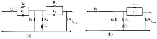
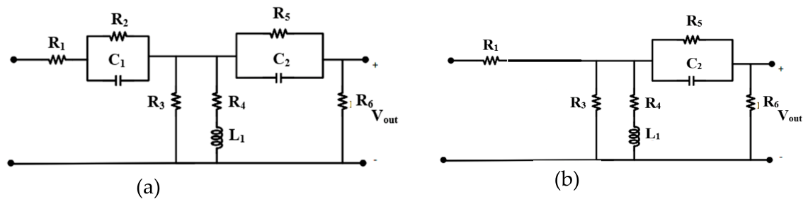
Consider the third-order RLC circuit shown in Figure 11a. The circuit contains two capacitors, C1 and C2, and one inductor, L1. The output voltage is measured across the indicated output terminals.
Figure 11.
(a) Third-order RLC network used to illustrate the systematic construction of the transfer function zero polynomial. (b) Reduced topology obtained from the circuit in Figure 11 by setting L1 = 0 and evaluating the limiting case C1 → ∞.
To calculate the coefficient of s, each energy storage element is considered individually. First, C1 is retained, while C2 and L1 are assigned their zero values. The corresponding first-order zero equation is
1 + R2C1s = 0.
Next, only the inductor L1 is retained. The reduced network gives
Finally, retaining only C2 results in
1 + R5C2s = 0.
The individual first-order contributions in (37)–(39) are combined to obtain the coefficient of s. Accordingly, the third-order zero polynomial can initially be written as
The second-order coefficient B is determined by considering all pairwise combinations of the energy storage elements. First, let L1 = 0, so that only C1 and C2 remain. The zero polynomial of the resulting second-order circuit can be expressed as
where B′ is the resistance-product factor to be determined.
1 + (R2C1 + R5C2)s + B′C1C2s2 = 0,
To reduce the order of this polynomial, C1 is allowed to approach infinity. The corresponding reduced topology is shown in Figure 10b.
Dividing the left-hand side of (41) by C1 and evaluating the limit gives
which reduces to
R2s + B′C2s2 = 0.
The remaining first-order network is governed by (43). To establish equivalence between the reduced forms, (43) is multiplied by R2s, yielding
R2s(1 + R5C2s) = R2s + B′C2s2.
Comparison of the coefficients of C2s2 gives
B′ = R2R5.
The same procedure is applied to the two remaining pairs, namely (C1, L1) and (C2, L1). Combining the contributions of all three pairs produces
The third-order coefficient C is obtained by simultaneously retaining all three energy storage elements and performing one additional order-reduction step. The result is
Substitution of (46) and (47) into (40) gives the complete zero polynomial:
In this example, the polynomial in (48) can equivalently be factorized as
Its roots are therefore
These roots contribute independently to the coefficients of the zero polynomial. This independence results from the topology of the corresponding reduced networks: series branches become isolated under open-circuit conditions, whereas parallel branches become isolated under short-circuit conditions. For circuit configurations exhibiting this separability, the zeros can be obtained directly from the associated first-order time constants without explicitly expanding the complete numerator polynomial.
For more strongly coupled circuits, however, the zero polynomial may not factor into independent first-order terms. In such cases, the pairwise and higher-order order-reduction procedure provides a systematic means of determining the polynomial coefficients before calculating its roots.
4.2. Extension to General Linear Circuits
Because transfer function zeros are the roots of the numerator polynomial, their calculation requires consideration of the selected input and output variables. Unlike poles, which are associated with the natural modes of the circuit, zeros depend on how the circuit is excited and where its response is observed. Consequently, a given circuit may exhibit different zeros for different transfer functions.
Several complementary approaches can be used to identify or calculate transfer function zeros.
4.2.1. Direct Circuit Analysis
The first approach is to derive the transfer function using conventional circuit analysis techniques, such as Kirchhoff’s current law, Kirchhoff’s voltage law, nodal analysis, or mesh analysis. After obtaining the transfer function, the numerator polynomial is set equal to zero.
Although this procedure is general, it can require extensive symbolic manipulation even for circuits of moderate order. The complexity increases further when the network contains dependent sources, multiple feedback paths, coupled energy storage elements, or transistor small-signal models. Direct derivation is therefore most useful for relatively simple circuits or for independently verifying a result obtained using the proposed method.
4.2.2. Magnitude-Based Identification of a Single Zero
When a transfer function contains only one finite zero and its influence can be considered independently of nearby poles, the zero frequency may be identified from the magnitude response. Consider
At zero frequency, its magnitude is
|H(s)|s=0 = ADC0.
For s = jω, the magnitude is
At ω = ∣z1∣, the magnitude becomes
Thus, for an isolated first-order zero, the break frequency corresponds to the frequency at which the magnitude is times its low-frequency value, equivalent to an increase of approximately 3 dB. This magnitude-based method identifies the absolute zero frequency but does not distinguish between left-half-plane and right-half-plane zeros because both produce the same magnitude response. Their distinction requires phase information or direct analytical evaluation.
4.2.3. Output-Nulling Condition
A transfer function zero may also be found by determining the frequency at which the output variable becomes zero despite a nonzero input excitation. Under this condition, the selected output node may be treated as a virtual ground when the output is a voltage. The resulting circuit equations can then be solved for the complex frequency s = sz that satisfies the output-nulling condition.
This method is particularly effective for circuits containing one dominant transmission zero. It also provides physical insight into the cancelation mechanisms responsible for the zero. For example, a zero may occur when two signal paths deliver equal-magnitude but opposite-phase contributions to the output node.
4.2.4. Transmission-Path Interruption
Another useful interpretation is based on the interruption of signal transmission between the input and output. If, at a particular complex frequency, the effective transfer path is opened or the input contribution is completely canceled before reaching the output, the circuit exhibits a transmission zero.
This condition may arise from an infinite branch impedance, a zero branch impedance that diverts the signal away from the output, or destructive cancelation between multiple feedforward and feedback paths. Examining such conditions can substantially simplify zero calculation in circuits whose topology clearly reveals the relevant signal paths.
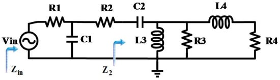
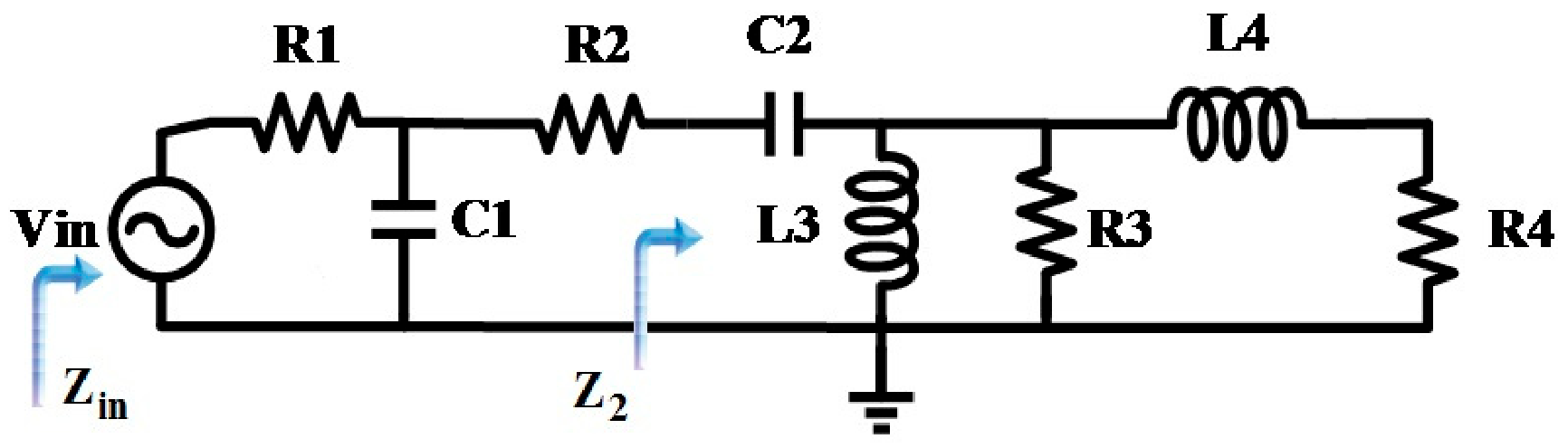
The preceding approaches may accelerate the analysis of specific circuit configurations. Nevertheless, they do not always provide a systematic simplification for higher-order networks. As an example, consider the fourth-order circuit shown in Figure 12, previously analyzed in [25]. This network contains two capacitors and two inductors arranged in a topology for which direct calculation of the input impedance results in a lengthy symbolic expression.
Figure 12.
Fourth-order RLC network used to compare direct symbolic derivation with the proposed coefficient-based order-reduction method [25].
To apply conventional impedance analysis, first define the equivalent impedance of the right-hand subnetwork as
The input impedance can then be expressed as
For a more compact representation, define
P(s) = R3L3s + (R3 + L3s)(L4s + R4)
And
such that Z2 = Q(s)/P(s). Substituting (58) into (48) and collecting the terms gives
Q(s) = R3L3s(L4s + R4),
Although the compact form in (59) is suitable for symbolic manipulation, full expansion of its numerator produces a fourth-order polynomial. After normalization, the zero polynomial is
Equation (59) demonstrates the amount of symbolic manipulation required by direct impedance expansion. Even though the original circuit contains only four energy storage elements, the resulting polynomial includes numerous products of resistances, capacitances, and inductances.
Alternatively, the normalized fourth-order polynomial can be expressed in the general form
1 + As + Bs2 + Cs3 + Ds4 = 0.
Using the order-reduction procedure, the first-order coefficient is calculated directly from the individual contributions of the energy storage elements:
where is the equivalent resistance observed from the terminals of capacitor Ci, and is the equivalent resistance associated with inductor Li. When evaluating each equivalent resistance, the other energy storage elements are assigned their zero values, while independent sources are deactivated and dependent sources remain active.
The higher-order coefficients B, C, and D are then obtained by considering all relevant pairs, triplets, and quadruplets of energy storage elements, respectively. In this manner, the complete polynomial can be constructed without first deriving and expanding the full input impedance. This coefficient-based approach preserves the explicit relationship between the polynomial terms and the corresponding circuit elements.
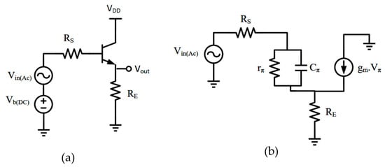
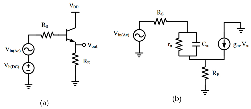
Nevertheless, direct output-nulling or signal-path arguments can be more efficient for circuit topologies in which the cancelation mechanism is readily identifiable. Consider, for example, the common-collector amplifier shown in Figure 13a and its high-frequency small-signal equivalent circuit in Figure 13b.
Figure 13.
Common-collector amplifier used to demonstrate direct zero calculation: (a) transistor-level circuit and (b) high-frequency small-signal equivalent model.
A zero occurs when the output current, and consequently the emitter current, becomes zero despite the presence of a nonzero input excitation. Applying this output-nulling condition to the small-signal model gives
Using
Equation (63) becomes
1 + rπCπs = −gmrπ.
The corresponding zero is therefore
here the approximation applies when gmrπ≫1.
This example illustrates that the most efficient zero-calculation strategy depends on the circuit topology. When a clear output-nulling or signal-cancelation condition is available, the zero may be obtained directly. For general higher-order networks, however, the proposed order-reduction method provides a systematic framework for constructing the zero polynomial while avoiding the complete symbolic expansion of the circuit equations.
5. Discussion
A recent approach [28] computes approximate symbolic pole/zero expressions valid near a specified design point by combining open-/short-circuit element replacement, state-matrix order reduction, and symbolic LR iterations, implemented in MAPLE. While effective, this approach targets one pole or zero per run, generally requires several seconds to a few minutes of computation per p/z (e.g., 2.33 min for a single pole in a ninth-order amplifier), and, by the authors’ own account, remains slower than commercial alternatives such as Analog Insydes. Likewise, an ensemble heuristic–metaheuristic method [29] simplifies symbolic pole/zero expressions of operational transconductance amplifiers by combining root splitting with a simulated-annealing-based optimization stage implemented in MATLAB. Both of these recent approaches, together with the LR- and optimization-based techniques discussed above, share a common requirement: iterative numerical or metaheuristic refinement carried out with dedicated symbolic-computation or optimization software. In contrast, the method proposed in this paper derives the full characteristic and zero polynomials of the network directly, through closed-form time constant summation and network-order reduction performed by hand, without iterative numerical refinement or optimization; a numerical solver (e.g., MATLAB) is needed only to extract the polynomial roots once the exact coefficients are known.
In contrast, the method proposed in this paper yields the exact analytical coefficients of the characteristic and zero polynomials—not an approximation with a bounded error—obtained directly through closed-form time constant summation and network-order reduction performed by hand, without iterative numerical refinement, metaheuristic optimization, or dedicated symbolic-computation software; a numerical solver (e.g., MATLAB) is needed only to extract the polynomial roots once these exact coefficients are known. Because the coefficients are exact rather than approximated locally, the resulting expressions remain valid over the full parameter space rather than being restricted to the neighborhood of a single design point, avoiding the need for multiple formulas at different design points as required in [28]. Furthermore, the proposed procedure obtains all poles (or zeros) of the network in a single, systematic pass, rather than requiring a separate run per targeted eigenvalue as in [28,29]. Finally, by relying on simple, interpretable operations rather than iterative or heuristic search, the method avoids the growing symbolic complexity and convergence/runtime limitations reported for LR-iteration- and metaheuristic-based approaches, while remaining transparent, exact, and easy to apply by hand even for higher-order networks.
Although the proposed order-reduction procedure is general and applies in principle to any linear time-invariant (LTI) network, several practical limitations should be noted. First, the number of required equivalent-resistance and time constant evaluations grows with the number of energy storage elements, so that purely manual application becomes increasingly demanding for very large-scale circuits containing tens of such elements; a systematic study of this regime has not been undertaken here and is left for future work. Second, excess-element configurations, such as capacitor loops or inductor cutsets, require explicit recognition and treatment through the auxiliary limiting-resistor technique illustrated in this paper, rather than being handled automatically. Finally, the method as presented is restricted to linear time-invariant circuits and small-signal equivalent models; nonlinear or time-varying circuits fall outside its current scope.
6. Conclusions
This paper presented a generalized order-reduction method for determining the transfer function coefficients, poles, and zeros of linear analog circuits. The proposed framework constructs the characteristic and zero polynomials by decomposing a higher-order network into reduced-order configurations and evaluating the contributions of individual energy storage elements and their combinations. In this manner, first-order coefficients are obtained from the associated equivalent resistances and time constants, whereas higher-order coefficients are determined through successive network-order reduction.
The method extends the previously developed characteristic-function analysis to the systematic calculation of transfer function zeros. The reciprocal relationship between driving-point impedance and admittance was used to formulate zero determination as a related pole-calculation problem. In addition, output-nulling, signal-path interruption, and magnitude-response interpretations were discussed as complementary techniques for circuits in which the zero-generating mechanism can be identified directly.
Representative RC, RLC, and transistor small-signal circuits were considered to illustrate the application of the method. The presented examples show that the proposed approach can accommodate passive and active networks containing capacitors, inductors, and dependent sources. Compared with direct nodal, mesh, or impedance-based expansion, the method can reduce the required symbolic manipulation while retaining explicit relationships between circuit parameters and polynomial coefficients. These parametric expressions provide useful design insight by allowing the influence of individual components on pole and zero locations to be examined directly.
The proposed framework is particularly useful for symbolic and design-oriented analysis of higher-order linear analog circuits. For networks with well-separated roots, reduced first-order models can also provide practical estimates of individual pole and zero locations. When roots are closely spaced or strongly coupled, the complete polynomial obtained using the proposed procedure should be solved to determine their accurate locations. Overall, the method provides a systematic complement to conventional circuit analysis techniques and establishes a unified basis for the efficient pole–zero characterization of linear analog networks.
While the illustrative examples in this paper involve networks of moderate order, the coefficient-derivation procedure itself does not assume a particular circuit size; a systematic study of very large-scale or highly complex circuits, containing tens of energy storage elements, is left as a direction for future work.
Author Contributions
Conceptualization, A.F. and S.A.; methodology, A.F. and S.A.; validation, A.F., S.A. and M.M.; formal analysis, M.M., M.M.G. and H.T.; resources, M.M.G. and H.T.; writing—original draft preparation, A.F. and S.A.; writing—review and editing, A.F., S.A. M.M., H.T. and A.K.; supervision, A.K. All authors have read and agreed to the published version of the manuscript.
Funding
This research received no external funding.
Institutional Review Board Statement
Not applicable.
Informed Consent Statement
Not applicable.
Data Availability Statement
The original contributions presented in this study are included in the article. Further inquiries can be directed to the corresponding authors.
Acknowledgments
During the preparation of this manuscript, the authors used ChatGPT (GPT-5.5; OpenAI, San Francisco, CA, USA) for the purpose of proofreading. The authors have reviewed and edited the output and take full responsibility for the content of this publication.
Conflicts of Interest
The authors declare no conflicts of interest.
Abbreviations
The following abbreviations are used in this manuscript:
| LTI | Linear Time-Invariant |
| OCTC | Open Circuit Time Constant |
| RC | Resistive-Capacitive |
| SCTC | Short Circuit Time Constant |
| ZVTC | Zero Value Time Constant |
References
- Bode, H.W. Network Analysis and Feedback Amplifier Design; Van Nostrand: New York, NY, USA, 1945. [Google Scholar]
- Elmore, W.C. The transient response of damped linear network with particular regard to wideband amplifiers. J. Appl. Phys. 1948, 19, 55–63. [Google Scholar] [CrossRef] [Scilit]
- Mulligan, J.H. The effect of pole and zero locations on the transient response of linear dynamic systems. Proc. IRE 1949, 37, 516–529. [Google Scholar] [CrossRef] [Scilit]
- Guillemin, E.A. Introductory Circuit Theory; Wiley: New York, NY, USA, 1953. [Google Scholar]
- Pederson, D.O.; Wilson, G.H. Dominant zero and excess phase of a Hurwitz polynomial. IEEE Trans. Circuits Syst. 1964, 11, 104–108. [Google Scholar] [CrossRef] [Scilit]
- Searle, C.L.; Boothroyd, A.R.; Angelo, E.J.; Gray, P.E.; Pederson, D.O. Elementary Circuit Properties of Transistors; Wiley: New York, NY, USA, 1964. [Google Scholar]
- Thornton, R.D.; Searle, C.L.; Pederson, D.O.; Adler, R.B.; Angelo, E.J. Multistage Transistor Circuits; Wiley: Hoboken, NJ, USA, 1965. [Google Scholar]
- Cochrun, B.L.; Grabel, A. A method for the determination of the transfer function of electronic circuits. IEEE Trans. Circuit Theory 1973, 20, 16–20. [Google Scholar] [CrossRef] [Scilit]
- Davis, A.M. Analyze active-network responses without complex manipulations. EDN Mag.-Electr. Des. News 1979, 24, 109–112. [Google Scholar]
- Davis, A.M.; Moustakas, E.A. Decomposition analysis of active networks. Int. J. Electron. 1979, 46, 449–456. [Google Scholar] [CrossRef] [Scilit]
- Davis, A.M.; Moustakas, E.A. Analysis of active RC networks by decomposition. IEEE Trans. Circuits Syst. 1980, 27, 417–419. [Google Scholar] [CrossRef]
- Rubinstein, J.; Penfield, P.; Horowitz, M.A. Signal delay in RC tree networks. IEEE Trans. Comput.-Aided Des. 1983, 2, 202–211. [Google Scholar] [CrossRef] [Scilit]
- Gray, P.R.; Meyer, R.G. Analysis and Design of Analog Integrated Circuits, 2nd ed.; Wiley: New York, NY, USA, 1984. [Google Scholar]
- Rosenstark, S. Feedback Amplifier Principles; MacMillan: New York, NY, USA, 1986. [Google Scholar]
- Middlebrook, R.D. Null double injection and the extra element theorem. IEEE Trans. Educ. 1989, 32, 167–180. [Google Scholar] [CrossRef] [Scilit]
- Fox, R.M.; Lee, S.G. Extension of the open-circuit time-constant method to allow for transcapacitances. IEEE Trans. Circuits Syst. 1990, 37, 1167–1171. [Google Scholar] [CrossRef] [Scilit]
- Thompson, M.T. Design linear circuits using OCTC calculations. Electron. Des.-Analog. Appl. Issue 1993, 41–47. [Google Scholar]
- Thompson, M.T. SCTC analysis estimates low-frequency -3 dB point. Electron. Des. 1993, 41, 65. [Google Scholar]
- Thompson, M.T. Chapter 6—Amplifier Bandwidth Estimation Techniques. In Intuitive Analog Circuit Design, 2nd ed.; Newnes: Oxford, UK, 2014; pp. 167–208. [Google Scholar]
- Andreani, P.; Mattisson, S. Characteristic polynomial and zero polynomial with the Cochrun-Grabel method. Int. J. Circ. Theor. Appl. 1998, 26, 287–292. [Google Scholar] [CrossRef]
- Middlebrook, R.D.; Vorperian, V.; Lindal, J. The N extra element theorem. IEEE Trans. Circuits Syst. I 1998, 45, 919–935. [Google Scholar] [CrossRef] [Scilit]
- Andreani, P.; Mattisson, S. Extension of the Cochrun-Grabel method to allow for mutual inductances. IEEE Trans. Circuits Syst. I Fundam. Theory Appl. 1999, 46, 481–483. [Google Scholar] [CrossRef] [Scilit]
- Salvatori, S.; Conte, G. On the SCTC-OCTC Method for the Analysis and Design of Circuits. IEEE Trans. Educ. 2009, 52, 318–327. [Google Scholar] [CrossRef] [Scilit]
- Hajimiri, A. Generalized time-and transfer-constant circuit analysis. IEEE Trans. Circuits Syst. I Regul. Pap. 2010, 57, 1105–1121. [Google Scholar] [CrossRef] [Scilit]
- Fathi, A.; Khoei, A.; Mousazadeh, M. Generalized method of analog circuit characteristic function analysis. IEEE Trans. Circuits Syst. II Express Briefs 2018, 66, 172–176. [Google Scholar] [CrossRef] [Scilit]
- Tavakkoli, H.; Duan, M.; Zhao, X.; Qi, L.; Ke, Z.; Izhar; Bermak, A.; Lee, Y.-K. A CMOS Hybrid Magnetic Field Sensor for Real-Time Speed Monitoring. IEEE Sens. J. 2022, 22, 22529–22539. [Google Scholar] [CrossRef] [Scilit]
- Tavakkoli, H.; Ahmed, M.; Shah, I.; Fang, S.; Chen, W.; Bermak, A.; Lee, Y.-K. An Integrated CMOS Micro Search-Coil Magnetometer with On-Chip Calibration and a Low-Noise Amplifier. Microsyst. Nanoeng. 2026, 12, 229. [Google Scholar] [CrossRef] [Scilit] [PubMed]
- Gheorghe, A.G.; Constantinescu, F. An Algorithm for Finding Approximate Symbolic Pole/Zero Expressions. Mathematics 2025, 13, 3314. [Google Scholar] [CrossRef] [Scilit]
- Behmanesh-Fard, N.; Yazdanjouei, H.; Shokouhifar, M.; Werner, F. Mathematical Circuit Root Simplification Using an Ensemble Heuristic–Metaheuristic Algorithm. Mathematics 2023, 11, 1498. [Google Scholar] [CrossRef] [Scilit]
Disclaimer/Publisher’s Note: The statements, opinions and data contained in all publications are solely those of the individual author(s) and contributor(s) and not of MDPI and/or the editor(s). MDPI and/or the editor(s) disclaim responsibility for any injury to people or property resulting from any ideas, methods, instructions or products referred to in the content. |
© 2026 by the authors. Licensee MDPI, Basel, Switzerland. This article is an open access article distributed under the terms and conditions of the Creative Commons Attribution (CC BY) license.