Performance Prediction of Long-Term Anaerobic Digestion Operation of Food Waste Using a Combined Approach of Time-Series Analysis Techniques and Biomethane Potential Test Results

Abstract

Predicting long-term anaerobic digestion (AD) performance for food waste remains challenging because of substrate variability, process disturbance, and limited routine monitoring data. This study developed a practical framework that combines biomethane potential (BMP) test results with time-series analyses to estimate methane production during steady-state long-term AD operation. Ten paired batch and long-term datasets from three research groups were analysed. Among four BMP kinetic models, the Cone model gave the best fit in eight of 10 datasets. For long-term prediction, a 3-day sliding-window method and two Kalman filter approaches were compared. The one-dimensional Kalman filter achieved the best overall predictive accuracy, while the two-dimensional Kalman filter, which incorporated substrate conversion efficiency, provided clearer identification of persistent abnormal deviations associated with potential inhibition. The proposed framework offers a simple and localised decision support tool for methane forecasting, noise reduction, and early warning of instability when only BMP data and routine methane measurements are available.

1. Introduction

Approximately 1.3 billion tons, which constitutes about one-third of the global food production, is lost or wasted throughout the food supply chain annually [1,2]. Food waste, whether in the form of precooked meals or leftovers, is unique among the category of municipal solid waste, owing to its feature of high moisture, salinity, organic matter, and oil content. To date, the common fate of this waste has been landfill, incineration, or composting [3]. In comparison to these traditional disposal methods, anaerobic digestion (AD) offers significant environmental benefits, including renewable energy generation, greenhouse gas capture, as well as nutrient recycling [4,5,6]. In reality, an accurate estimation of the performance of an AD system treating food waste is crucial for process optimisation, operational planning, and resource management [7,8]. However, the existing approaches face challenges owing to the variability of food waste as a substrate, the complex and nonlinear nature of the AD process, and limitations of relying solely on the data collected from individual systems [2,9].

Experimental evaluation of AD performance is commonly carried out using either batch tests or long-term (semi-)continuous operations. Among batch methods, the biochemical methane potential (BMP) test is widely used to estimate the ultimate methane yield of a substrate and to provide initial information on substrate degradation and methane production kinetics. BMP tests are attractive because they are comparatively simple, less resource-intensive, and easier to standardise than long-term reactor experiments [10]. Meanwhile, recent work highlights that BMP interpretation depends strongly on test design, inoculum quality, termination criteria, and inter-laboratory consistency, so ongoing standardisation remains important for using BMP results as predictive inputs for process design and modelling [11,12].

Long-term AD operation provides a more realistic picture of process stability, adaptation, and response to operational changes, including shifts in organic loading rate (OLR), feedstock composition, and additive dosage [13,14]. Consequently, a broad range of prediction approaches has been developed for long-term AD performance (Table 1). Mechanistic models, particularly ADM1-based frameworks, remain the reference approach for representing biochemical pathways and intermediate transformations in AD, but they typically require extensive parameterization, calibration, and process state measurements that are not always available in routine operations [15]. Machine learning models have become increasingly popular for biogas and methane prediction because they can capture nonlinear relationships directly from the data [16,17]. However, these usually depend on relatively large, high-quality datasets and may have limited transferability across reactors or feedstocks [16,17]. Whilst hybrid approaches combining mechanistic and data-driven elements have been proposed to improve predictive accuracy while retaining some process interpretability, these approaches still tend to require substantial modelling effort and monitoring input [18].

BMP-based extrapolation provides a practical intermediate route between simple batch testing and fully mechanistic long-term modelling. Previous studies have used kinetic models fitted to BMP curves, scaling, or conversion factors, as well as simplified simulation frameworks to infer longer-term methane production from batch results [19,20,21]. However, these approaches remain affected by uncertainties in substrate composition, operating conditions, microbial adaptation, and process disturbances that are not fully captured by batch experiments alone [22,23,24,25]. Recent studies have also shown continued interest in combining kinetic information with newer predictive tools, including physics-informed and hybrid modelling strategies, to improve methane yield prediction from limited data [18,21].

Time-series analysis offers another practical route for prediction because it can update estimates recursively as new measurements become available [26]. In AD research, this includes both relatively simple lag window methods and state estimation approaches based on the Kalman filter or its nonlinear variants [27,28]. Recent work has shown the value of extended, unscented, and related robust Kalman filter approaches for handling dynamic AD systems and process control applications, while newer sequence models, including transformer-based time-series predictors, have also demonstrated strong forecasting performance for biogas production [29,30]. Moreover, many of these methods remain data-intensive or mathematically demanding, and their practical deployment can be difficult when only a limited set of routine methane measurements is available.

Time-series analysis techniques, such as the lag method and Kalman filter, serve not only to provide a prediction interval for the evaluation stages but also to estimate the state of a dynamic system as it evolves over time [27,28]. Both approaches rely on recursive mathematical algorithms that blend information from a series of measurements with a mathematical model of the system. This integration enables them to generate predictions of the system state and the associated uncertainties at each time step [29,31].

Table 1. Overview of mainstream approaches for predicting anaerobic digestion performance and their main advantages and limitations.

Model Category	Typical Application in AD	Main Advantages	Main Limitations	Relevance to This Study	Reference
Mechanistic models (e.g., ADM1)	Simulation of biochemical pathways, intermediate dynamics, and process control.	Strong process interpretability; can represent substrate degradation and intermediate formation explicitly.	Require substantial parameterisation, calibration, and process state measurements; often difficult to apply with limited routine data.	Serve as an important benchmark in the literature but are often too data-intensive for the practical prediction setting targeted here.	[24]
Machine learning models	Methane/biogas prediction, soft sensing, fault detection, forecasting from operational data.	Can capture nonlinear relationships directly from data; often high predictive accuracy when large datasets are available.	Depend on large, high-quality datasets; lower interpretability; transferability across reactors/feedstocks may be limited.	Relevant as advanced predictors, but less suitable when only limited literature-derived or routine methane data are available.	[16,17]
Hybrid models	Combining process knowledge with data-driven correction or optimisation.	Improved predictive performance while retaining some process interpretability.	Still require substantial modelling effort and monitoring inputs; implementation complexity remains high.	Useful for future extension, but beyond the intended simplicity of the present framework.	[18]
BMP-based kinetic models	Using batch BMP results to estimate methane potential and longer-term performance.	Practical, low-cost, and compatible with commonly available batch test data.	May not fully capture long-term microbial adaptation, operational variability, or inhibition dynamics.	Forms one of the main foundations of the present study.	[19,20,21]
Time-series methods (lag method, Kalman filter)	Recursive updating, noise reduction, short-term forecasting, state estimation.	Useful when measurements are limited; can provide localised prediction and uncertainty handling.	Depend on assumptions regarding state evolution and noise; less suitable for highly nonlinear or disturbed systems.	Core focus of the present study, especially for steady-state operation.	[26,27,28]

Table 1. Overview of mainstream approaches for predicting anaerobic digestion performance and their main advantages and limitations.

Model Category	Typical Application in AD	Main Advantages	Main Limitations	Relevance to This Study	Reference
Mechanistic models (e.g., ADM1)	Simulation of biochemical pathways, intermediate dynamics, and process control.	Strong process interpretability; can represent substrate degradation and intermediate formation explicitly.	Require substantial parameterisation, calibration, and process state measurements; often difficult to apply with limited routine data.	Serve as an important benchmark in the literature but are often too data-intensive for the practical prediction setting targeted here.	[24]
Machine learning models	Methane/biogas prediction, soft sensing, fault detection, forecasting from operational data.	Can capture nonlinear relationships directly from data; often high predictive accuracy when large datasets are available.	Depend on large, high-quality datasets; lower interpretability; transferability across reactors/feedstocks may be limited.	Relevant as advanced predictors, but less suitable when only limited literature-derived or routine methane data are available.	[16,17]
Hybrid models	Combining process knowledge with data-driven correction or optimisation.	Improved predictive performance while retaining some process interpretability.	Still require substantial modelling effort and monitoring inputs; implementation complexity remains high.	Useful for future extension, but beyond the intended simplicity of the present framework.	[18]
BMP-based kinetic models	Using batch BMP results to estimate methane potential and longer-term performance.	Practical, low-cost, and compatible with commonly available batch test data.	May not fully capture long-term microbial adaptation, operational variability, or inhibition dynamics.	Forms one of the main foundations of the present study.	[19,20,21]
Time-series methods (lag method, Kalman filter)	Recursive updating, noise reduction, short-term forecasting, state estimation.	Useful when measurements are limited; can provide localised prediction and uncertainty handling.	Depend on assumptions regarding state evolution and noise; less suitable for highly nonlinear or disturbed systems.	Core focus of the present study, especially for steady-state operation.	[26,27,28]

This study aimed to develop a practical procedure for estimating the performance of steady-state long-term AD operation by combining BMP test results with time-series analysis techniques using literature-derived methane production datasets [32,33,34,35]. The framework was not intended to reproduce the full nonlinear biochemical complexity of AD, but rather to provide localised performance prediction and noise reduction for comparatively stable operating periods. Accordingly, it was designed as a practical and localised prediction tool for steady-state operation, rather than as a universal model transferable to all AD systems without recalibration. The selected approaches were evaluated by comparing their ability to predict methane production using only a limited set of inputs that are more likely to be available in practice, including BMP results for the same or comparable feedstock, together with operational measurements from long-term digestion.

2. Results and Discussion

2.1. Simulating BMP Results with Kinetic Models

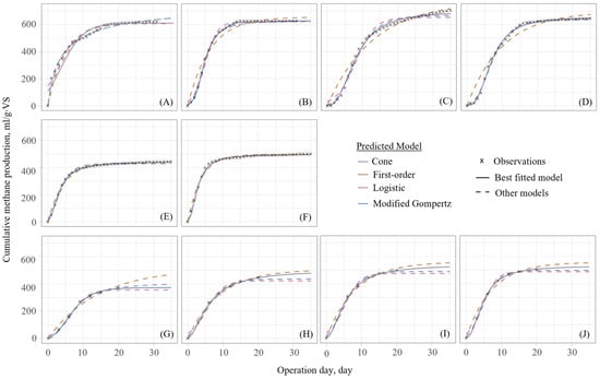
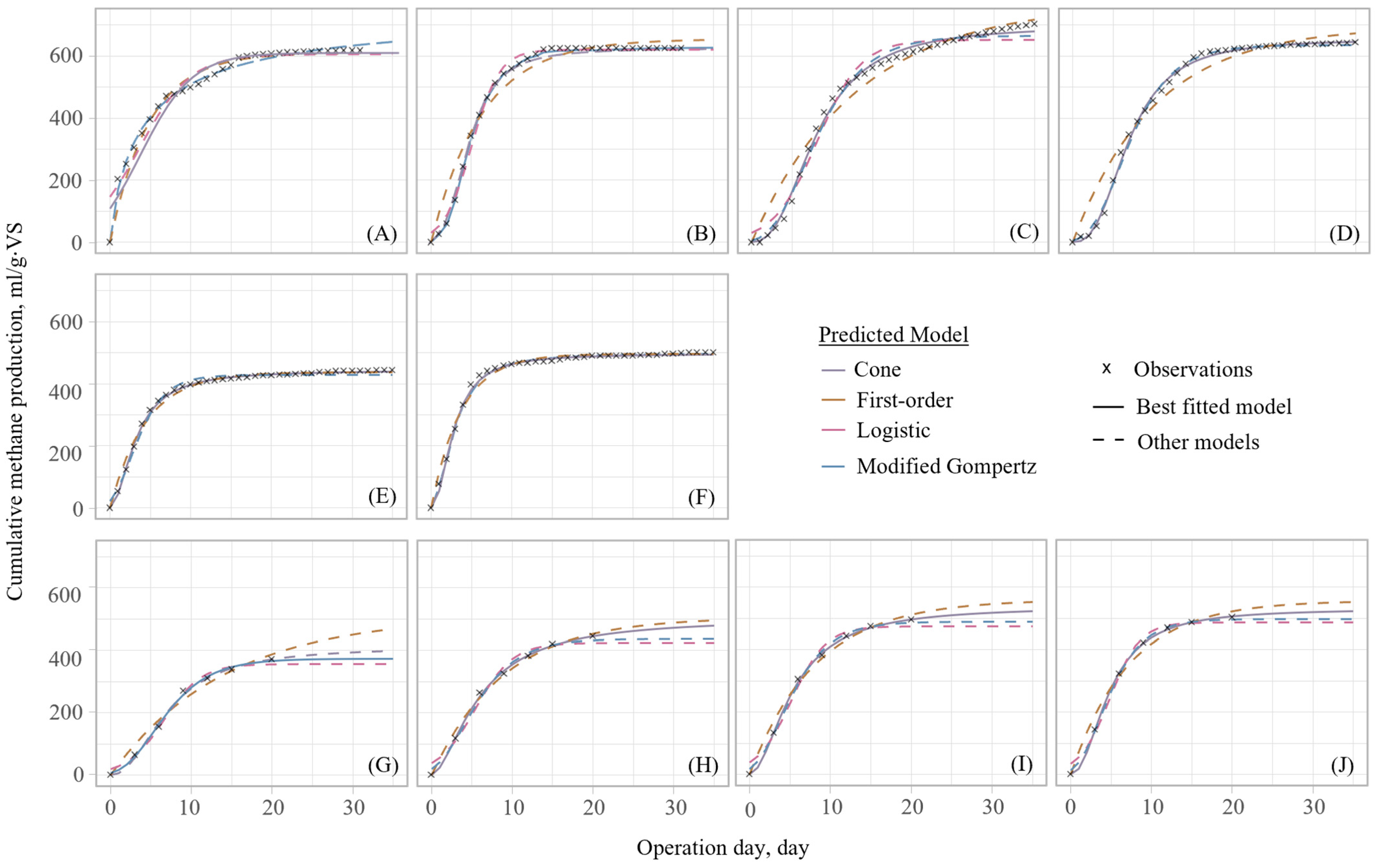
To capture cumulative methane production during batch BMP tests, four kinetic models, namely the first-order, modified Gompertz, logistic, and Cone models, were used to simulate cumulative methane production in the 10 batch BMP datasets included in this study [32,33,34,35]. The dataset details are summarised in Table 3, the fitted curves are shown in Figure 1, the parameters of the selected best-fit model are listed in Table 2, and the full model evaluation results are provided in Supplementary Table S1.

Figure 1. Fitting of selected kinetic models to cumulative methane production curves from batch BMP assays reported in different studies. The datasets include (A) Zhu food waste (Dataset I), (B) Zhu cellulose control (Dataset II), (C) Zhu cellulose with optimal nano-magnetite dosage (Dataset III), (D) Zhu cellulose with high nano-magnetite dosage (Dataset IV), (E) Tampio food waste (Dataset V), (F) Tampio autoclaved food waste (Dataset VI), (G) Zhang food waste baseline (Dataset VII), (H) Zhang food waste with 50% optimal metal supplementation (Dataset VIII), (I) Zhang food waste with 50% optimal metal supplementation plus EDDS (Dataset IX), and (J) Zhang food waste with 100% optimal metal supplementation (Dataset X).

Table 2. Summary of fitted kinetic parameters and best-fit model performance for the batch methane production curves shown in Figure 1.

Dataset	Best-Fit Model	Kinetic Model Parameters of Best-Fit Model 1				Best-Fit Model Performance Evaluation			Notes
		k, d−1	n	λ, d	G(t), mL/g·VS	R2	RMSE	AIC
I	Cone	0.24	0.86	-	645.57	0.99	13.08	170.56	Zhu food waste
II	Modified Gompertz	-	-	1.44	622.60	0.99	6.80	128.65	Zhu cellulose control
III	Cone	0.12	2.49	-	678.15	0.99	15.24	202.12	Zhu cellulose with optimal nano-magnetite dosage
IV	Cone	0.14	2.71	-	644.68	0.99	10.87	177.79	Zhu cellulose with high nano-magnetite dosage
V	Cone	0.31	1.89	-	439.06	0.99	4.12	107.98	Tampio food waste
VI	Cone	0.36	2.05	-	494.59	0.99	7.23	148.43	Tampio autoclaved food waste
VII	Modified Gompertz	-	-	1.55	397.59	0.99	7.87	34.88	Zhang food waste baseline
VIII	Cone	0.17	1367	-	477.62	0.99	6.05	31.2	Zhang food waste with 50% optimal metal supplementation
IX	Cone	0.19	1.88	-	523.62	0.99	5.12	28.87	Zhang food waste with 50% optimal metal supplementation plus EDDS
X	Cone	0.21	2.13	-	522.65	0.99	2.69	19.85	Zhang food waste with 100% optimal metal supplementation

¹ k and n stand for hydrolysis rate (d⁻¹) and shape factor for the Cone model, respectively; λ stands for lag phase (d) from modified Gompertz model.

Among the 10 datasets, the Cone model provided the best fit in 8 cases, whereas the modified Gompertz model performed best in the remaining 2 cases (Table 2 and Figure 1). Overall, the Cone model most consistently reproduced the observed methane accumulation curves, with the coefficient of determination (R²) values generally exceeding 0.99 (Table S1). This suggests that, for most of the substrates examined here, methane production was better described by a gradually curved and hydrolysis-governed accumulation pattern than by a strictly sigmoidal profile. Such behaviour is plausible for food waste, which is compositionally heterogeneous and often contains fractions with different degradability, leading to non-ideal cumulative methane production curves that are more flexibly captured by the Cone model through its shape factor $\mathrm{n}$ [20]. By contrast, the modified Gompertz model performed better in the case of cellulose-based substrate (dataset II, Figure 1B) and the food waste baseline from Zhang’s group (Dataset VII, Figure 1G), both of which exhibited a clearer lag phase at the beginning of digestion [20]. In these cases, the inclusion of the lag phase parameter λ allowed the modified Gompertz model to better represent microbial acclimation and delayed methane onset [20]. Notably, the datasets from Zhu and Tampio showed higher AIC values than those from Zhang, which may partly reflect the sensitivity of AIC to sample size and model complexity when more observations are available [36].

The fitted parameters k and λ from both modified Gompertz and Cone models provided useful indicators of substrate degradability and methane production process. Hydrolysis is often recognised as a rate-limiting stage of AD, particularly for particulate and cellulose-rich substrates [37]. In general, lower k values and longer λ values corresponded to slower degradation and delayed methane production. The cellulose control dataset (Dataset B) exhibited slower apparent kinetics than the food waste baseline (Dataset A). This is consistent with the more complex cellulose structure compared to food waste, which hinders the microbial and enzymatic deconstruction during the AD process [38]. In contrast, pretreatment or additive-amended datasets generally showed faster apparent kinetics, reflected by higher k values or shorter λ values, indicating accelerated substrate conversion. These trends support the interpretation that substrate composition and treatment condition strongly influenced BMP behaviour across the collected datasets [32,33,34,35].

2.2. Prediction Intervals of Long-Term AD Operation

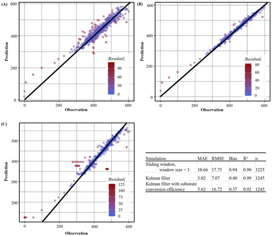
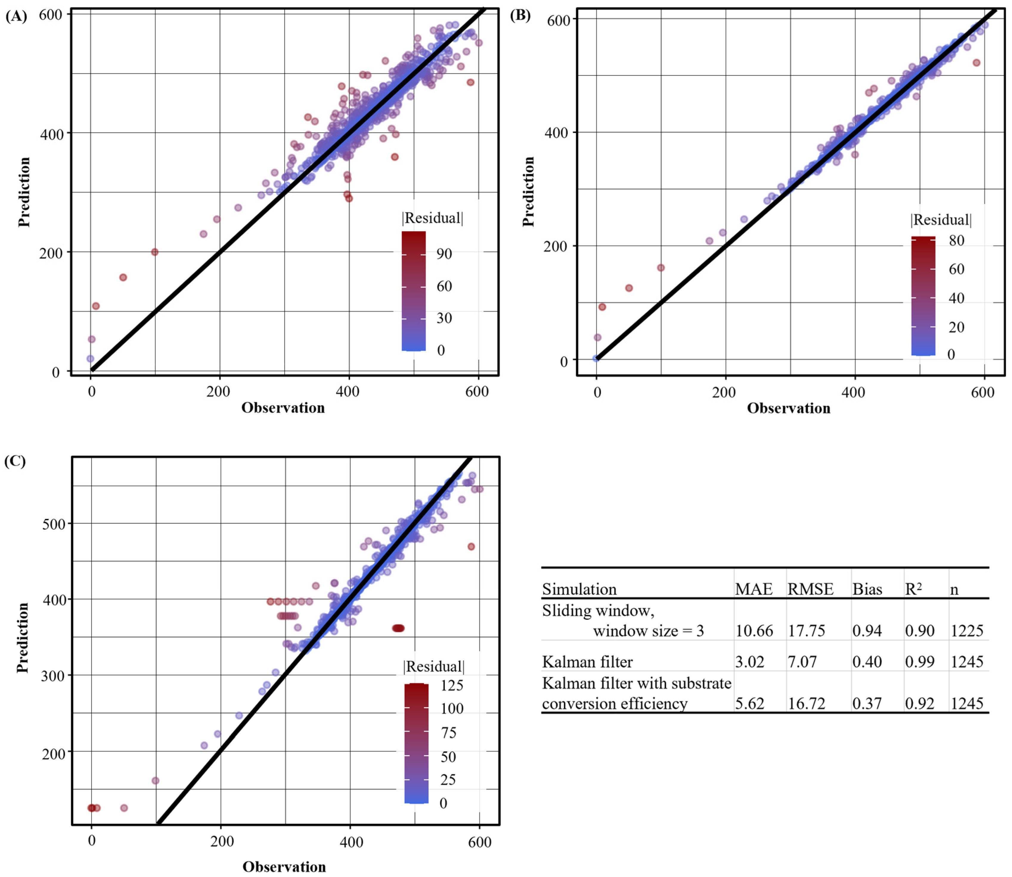
The performance of all the three approaches (sliding-window with a window size of 3 days, Kalman filter with constant methane production, and Kalman filter with substrate utilisation rate) are summarised in Figure 2, while the evaluations of all these three approaches for each dataset are presented in Supplementary Table S2. In general, the constant-yield Kalman filter (Section 2.2.2) was generally the most accurate of the three time-series approaches tested here, whereas the substrate-constrained Kalman filter (Section 2.2.3) offered a more mechanistically informed but less flexible alternative.

Figure 2. Scatter plot of predicted values vs observations across all datasets, derived from: (A) lag method; (B) one-dimensional Kalman filter with constant daily methane production rate; and (C) two-dimensional Kalman filter coupling substrate conversion efficiency.

2.2.1. Lag Method

The sliding-window method provided a simple and practical baseline for methane prediction, but its performance depended strongly on window size. The results suggest that a short window (3 days) is generally more suitable for capturing local methane production dynamics (Figure 2A), which is consistent with the short turnover time of volatile fatty acids (VFAs) in AD systems [39,40]. However, this approach remained sensitive to dataset-specific variability and offered limited robustness when longer smoothing windows were used.

Across the 10 datasets, the 3-day window generally gave the most accurate predictions, achieving the lowest mean absolute error (MAE) and root mean squared error (RMSE) in 8 out of 10 cases, whereas the 9-day window performed best only in Datasets III and IV (Supplementary Figure S1 and Table S3). Furthermore, the minimum hydraulic retention time (HRT) window did not provide the best MAE or RMSE in any dataset.

The advantage of the 3-day window was particularly evident for most of the datasets. For example, in Dataset V (Tampio food waste), the 3-day window gave an MAE of 5.13 and an RMSE of 6.72, compared with 10.29 and 13.43 for the 9-day window, and 18.34 and 21.90 for the minimum HRT window. A similar pattern was observed in Dataset VII (Zhang food waste baseline), where prediction error increased markedly with window size, from MAE = 21.59 and RMSE = 34.56 for the 3-day window to 66.78 and 104.47, respectively, for the HRT-based window. This observation suggests that, under relatively stable but still variable steady-state conditions, recent observations are the most informative for short-term methane prediction. In contrast, larger windows may over-smooth meaningful deviations in methane yield, including those associated with inhibition or changes induced by trace metal supplementation, thereby reducing predictive accuracy [32].

The only exceptions were Datasets III and IV, for which the 9-day window marginally outperformed the 3-day window in terms of both MAE and RMSE. These two datasets corresponded to cellulose-based systems with nano-magnetite addition, where methane production may have been influenced by additive-related process stabilisation and smoother substrate conversion dynamics. In such cases, a slightly broader short-term memory may better capture the underlying process than a very narrow window.

2.2.2. Kalman Filter with Constant Daily Methane Yield

In this approach, the Kalman filter used a one-dimensional hidden state representing the “true” daily methane production rate and recursively updated this state from the observed methane production data under the assumption of gradual state evolution during steady-state operation (Section 2.3). The overall comparison between observed and predicted methane production across all datasets is shown in Figure 2B, while the corresponding dataset-level evaluation results are provided in Supplementary Table S2. Across the 10 datasets, this approach consistently improved prediction accuracy relative to the three-day sliding-window method, yielding lower MAE and RMSE in every dataset.

The improvement was especially clear for datasets with relatively stable long-term behaviour. For example, in Dataset V (Tampio food waste), the Kalman filter reduced the MAE and RMSE from 5.13 and 6.72 using the 3-day sliding-window to 1.62 and 2.70, respectively. Similar improvements were observed in Datasets VIII, IX, and X, where the MAE values decreased to a range of 1.38 to 1.69 and the RMSE values to a range of 1.89 to 2.91, compared with noticeably larger errors obtained from the sliding-window approach. Even in the more difficult cellulose-based cases III and IV with nano-additives, the Kalman filter markedly improved performance, reducing RMSE from 15.46 and 20.61 to 7.47 and 9.96, respectively. These results suggest that recursive filtering was more effective than a purely local lag window average for removing measurement noise while preserving the underlying methane production signal. This is consistent with the established role of the Kalman filter as a recursive estimator that combines process evolution and observations to reduce measurement uncertainty in dynamic systems [27].

The main limitation of this implementation is that it relies entirely on observational updating and therefore does not constrain the methane production state using substrate-specific methane potential. Although this improves flexibility, it also introduces the possibility of overfitting, particularly when the filter adapts too closely to local measurement variation or dataset-specific noise. This may explain why some datasets still showed residual spread or positive bias, most notably Dataset VII (Zhang food waste baseline), where the MAE remained 10.66 and the RMSE 21.53. The consistently high R² values, generally above 0.94 and reaching 0.99 in several datasets, indicate that the approach captured the overall methane production pattern well. However, part of the apparent accuracy may reflect close adaptation to the observed series rather than fully generalisable prediction behaviour [29,30].

Overall, compared with the three-day sliding-window method, the one-dimensional Kalman filter provided a more robust and accurate baseline for steady-state methane prediction by combining local adaptability with recursive noise correction. Recent AD studies have similarly shown that Kalman filter-based state estimation can improve process prediction and tracking, particularly when only limited routine observations are available [29,30].

2.2.3. Kalman Filter with Constant Methane Yield and Substrate Conversion Efficiency

The second Kalman filter implementation extended the hidden state to two dimensions by jointly representing the daily methane production rate and the substrate conversion efficiency from relevant BMP test. This structure was intended to stabilise prediction by constraining the recursive update with both observed methane production and BMP-derived methane potential. The overall comparison across all datasets is shown in Figure 2C, and the detailed evaluation results are summarised in Supplementary Table S2.

The two-dimensional implementation yielded substantially better predictions than the sliding-window method in most cases and maintained relatively high R² values for several datasets. Meanwhile, though the implication of the second dimension retained useful noise removal capability, its benefits were more dataset-dependent than those of the simpler one-dimensional filter presented in previous section—Section 2.2.2. This outcome is consistent with broader AD state estimation studies, showing that additional model structure can improve estimation only when the embedded process assumptions remain well aligned with the actual operating dynamics [29,41].

For relatively stable datasets such as V, VIII, XI, and X, the two-dimensional Kalman filter performed well, with MAE values of 2.28, 1.89, 3.14, and 2.62, respectively. These errors were lower than those obtained with the sliding-window approach, although they remained consistently higher than those from the simpler one-dimensional Kalman filter. By contrast, larger prediction errors were generally observed in datasets with reported or suspected inhibition, suggesting that the inclusion of substrate conversion efficiency reduced the filter’s flexibility when the observed methane production pattern deviated from the idealised steady-state pattern implied by the corresponding BMP test. This effect was most pronounced in Dataset VI, where the RMSE increased to 26.36, compared with 3.79 for the one-dimensional Kalman filter and 20.96 for the three-day sliding-window. Although less extreme, drops in simulation performance were also observed in Datasets I, II, VII, IX, and X. These results suggest that coupling the filter with a BMP-derived conversion efficiency term may over-constrain the recursive update when long-term reactor behaviour is affected by instability or inhibition rather than by substrate conversion alone. More detailed interpretation of this relationship is provided in Section 2.3.

2.3. Predicted Trends of Long-Term AD Operation and Inhibition Forecast

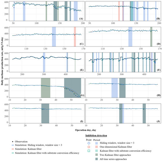
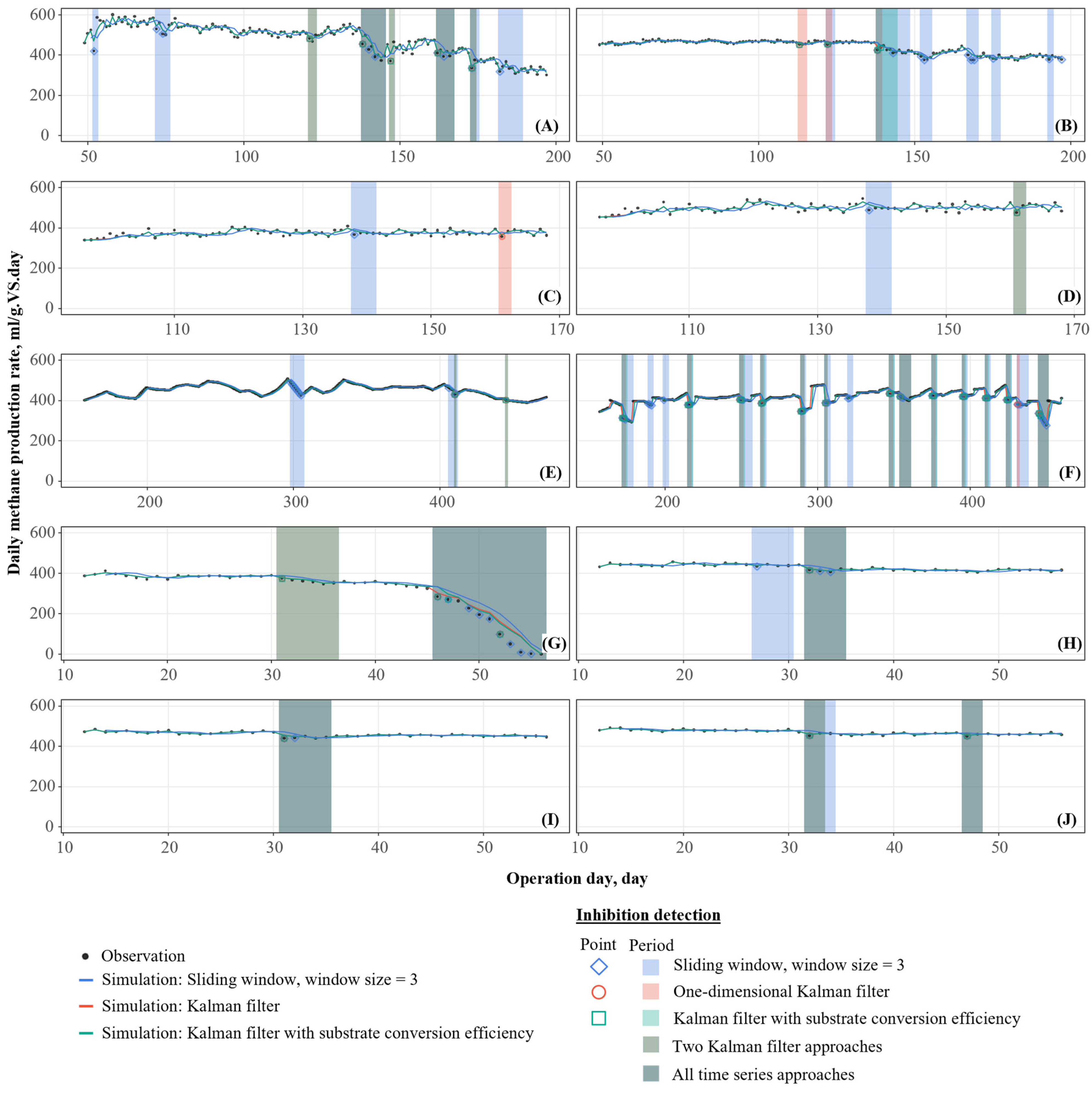
The three time-series approaches were further used to estimate pointwise methane production trends during long-term steady-state operation. As shown in Figure 3, the predicted trends are represented by coloured lines and the observed methane production values by points. The same figure also integrates the inhibition forecast results, allowing simultaneous comparison of trend tracking, noise removal, and disturbance identification. Overall, all three approaches captured the broad pattern of long-term methane production, but the two Kalman filter-based methods generally produced smoother and more accurate trend estimates than the 3-day sliding-window approach, particularly when the methane production trajectory was affected by measurement noise or temporary operational disturbance. Across the 10 datasets, the one-dimensional Kalman filter provided the most accurate overall trend reconstruction, consistent with its superior performance in Supplementary Table S2 and the results discussed in Section 2.2, while the two-dimensional Kalman filter was the most constrained by process assumptions. These differences became particularly important for inhibition forecasting, because excessive sensitivity may lead to fragmented or premature alarm periods, whereas excessive smoothness may delay recognition of true deterioration.

Figure 3. Predicted trend with measurement noise removal and inhibition forecast within each dataset: (A) Zhu food waste (Dataset I), (B) Zhu cellulose control (Dataset II), (C) Zhu cellulose with optimal nano-magnetite dosage (Dataset III), (D) Zhu cellulose with high nano-magnetite dosage (Dataset IV), (E) Tampio food waste (Dataset V), (F) Tampio autoclaved food waste (Dataset VI), (G) Zhang food waste baseline (Dataset VII), (H) Zhang food waste with 50% optimal metal supplementation (Dataset VIII), (I) Zhang food waste with 50% optimal metal supplementation plus EDDS (Dataset IX), and (J) Zhang food waste with 100% optimal metal supplementation (Dataset X).

The 3-day sliding-window method, although less accurate overall, still reproduced the general direction of methane production trends in the more stable datasets. Its main limitation was reduced robustness when the observations were noisy or when the process exhibited abrupt but short-lived deviations. Because this approach depends entirely on the most recent measurements, it reacted directly to local extremes and therefore produced trend estimates that were more sensitive to short-term fluctuations. This behaviour was already discussed in Section 2.2, where the sliding-window method showed higher MAE and RMSE values than both Kalman filter approaches across all datasets. In Figure 3, this sensitivity is reflected by sharper local deviations and less effective noise removal than in the Kalman filter-based trends. Such behaviour is expected from lag-based local averaging methods, which are useful for short-term smoothing but do not explicitly account for latent process evolution [9,28].

To convert the predicted trends into inhibition forecasts, time points were flagged when the observed methane production values deviated beyond the method-specific threshold, and periods with persistent outliers lasting more than three consecutive time steps were classified as potential inhibition periods. Because most datasets used a daily time step, this criterion corresponds approximately to the characteristic turnover time of VFAs, which are key short-term intermediates associated with methane production disruption in AD systems [39,40]. Isolated outliers that did not persist for at least three time steps were therefore interpreted as operational fluctuations rather than inhibition. Within this framework, the methods differed not only in trend reconstruction, but also in the consistency and interpretability of the flagged inhibition periods.

Based on the source studies, inhibition-related behaviour was reported in Datasets I, II, IV, VI, and VII [32,33,34,35]. These datasets showed either sustained abnormal deviations in methane production or repeated periods of depressed yield relative to the predicted steady-state trend, whilst the remaining datasets were comparatively stable and displayed only limited transient fluctuations during the evaluation phase. This distribution indicates that the prediction methods should be assessed not only by the goodness-of-fit metrics, but also by their ability to distinguish stable operation from persistent process deterioration.

In the inhibition-related datasets, the differences among methods became much more pronounced. The one-dimensional Kalman filter often adapted very closely to the observations, which improved goodness-of-fit metrics in some cases but also made the predicted trend highly sensitive to local measurement deviations. For example, in Figure 3C, where the estimated trend responds strongly to the observed series, a similar but more severe issue was observed for the sliding-window method, which relied entirely on recent measurements and therefore produced even more reactive and locally distorted trends in disturbance-affected datasets. In other words, both the one-dimensional Kalman filter and the sliding-window method could follow the observations closely, but part of this apparent responsiveness may reflect over-adaptation to short-term variation rather than robust representation of the underlying process state [9,42].

The two-dimensional Kalman filter, which involved substrate conversion efficiency as an additional state variable, generally produced smoother trend patterns and was less affected by isolated measurement fluctuations. This made it more conservative in its trend reconstruction, but also less flexible when the reactor behaviour deviated strongly from the BMP-implied conversion pattern. The clearest example is Dataset III (Figure 3C), for which no inhibition was reported in the source study [35]. In this case, both the sliding-window method and the one-dimensional Kalman filter were highly sensitive to local observations and therefore readily flagged the disturbed period, although this responsiveness also increased the risk of fragmented or overly reactive forecasts. Meanwhile, the two-dimensional Kalman filter produced a smoother and more persistent flagged period, suggesting that the additional substrate conversion constraint reduced sensitivity to short-term fluctuations. The biological and operational implications of these inhibition-related deviations are discussed further in Section 2.4.

2.4. Determinants of Model Precision

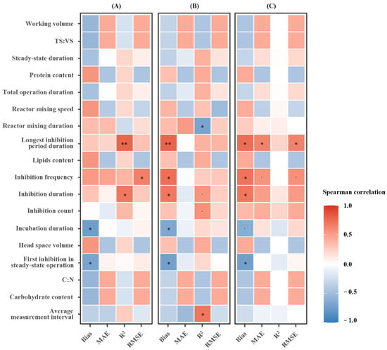
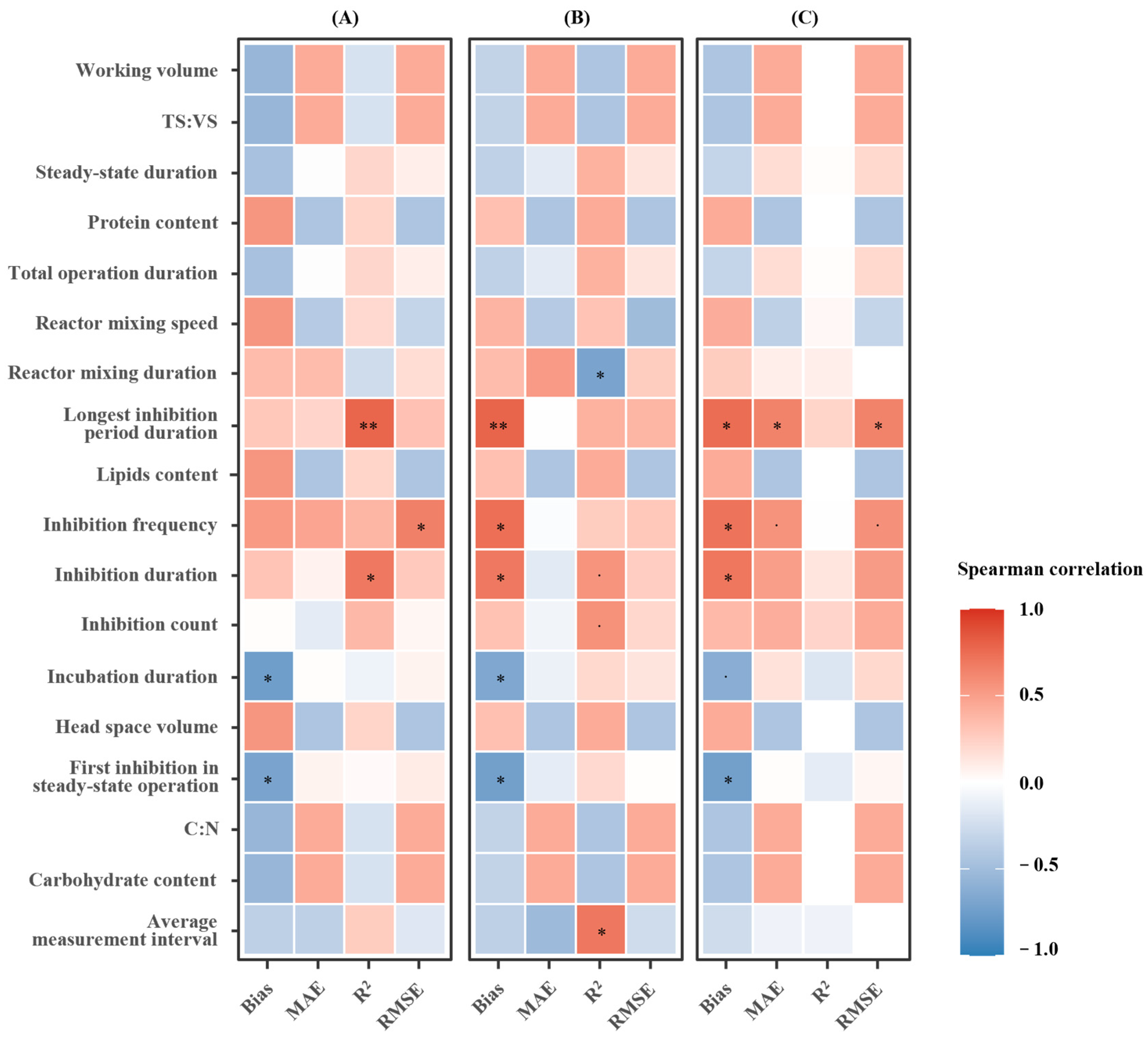
Figure 4 presents the correlations between selected operational or modelling-related parameters and the prediction accuracy of the three time-series approaches used in this study. To facilitate interpretation, the input parameters were grouped according to their relevance to substrate characteristics, operating conditions, measurement structure, system status, and modelling process. The ordering of variables in the matrix was determined by hierarchical clustering to group parameters with similar correlation patterns. Statistical significance was also evaluated, and markers shown in the matrix indicate the strength of the corresponding correlations.

Figure 4. Correlation matrix between the parameters and prediction accuracy. (A) Lag method; (B) one-dimensional Kalman filter with constant daily methane production rate; (C) two-dimensional Kalman filter coupling substrate conversion efficiency. Significance markers indicate the strength of the correlation, where “**” indicates p < 0.01, “*” indicates p < 0.05, and “.” indicates p < 0.1.

For the lag method (Figure 4A), the prediction accuracy was mainly associated with variables related to system instability, particularly inhibition-related indicators. Both inhibition frequency and inhibition duration were positively correlated with RMSE, indicating that the lag method became less accurate when the reactor experienced repeated or prolonged disturbance. A positive association was also observed between the longest inhibition period duration and both R² and error metrics, suggesting that extended disturbance periods strongly influenced the fitted trend and residual structure. Whilst relatively few strong correlations were observed between lag method performance and substrate composition or reactor design variables. This is consistent with the fact that the lag method relies only on recent observations and does not explicitly incorporate process-specific mechanistic information.

For the one-dimensional Kalman filter (Figure 4B), the correlation pattern was broader. In addition to inhibition-related variables, several measurement and operational factors showed associations with model accuracy. For example, average measurement interval was positively associated with bbias, indicating that prediction performance deteriorated when the time interval between observations increased. This is reasonable because the one-dimensional Kalman filter updates its hidden methane production state directly from the observed time series. Therefore, less frequent measurements reduce the filter’s ability to correct state estimates recursively. Inhibition-related variables, especially inhibition frequency and inhibition duration, were again positively related to bias and RMSE, confirming that process disturbance remained a major source of prediction uncertainty even when recursive state updating was used. Compared with the lag method, the one-dimensional Kalman filter appeared more sensitive to the temporal structure of the dataset, which reflects its stronger dependence on sequential observational updates.

The two-dimensional Kalman filter (Figure 4C), which incorporated substrate conversion efficiency as an additional state variable, showed the strongest relationships with inhibition-related indicators. Notably, longest inhibition period duration, inhibition frequency, and inhibition duration all presented positive associations with bias, MAE, and RMSE, suggesting that this approach was especially sensitive to persistent process deterioration. This result is consistent with earlier findings that the additional BMP-based process constraint improved the delineation of inhibition periods, but reduced flexibility when long-term reactor behaviour deviated from the expected substrate conversion pattern. In other words, when the system remained close to the steady-state trajectory implied by the BMP test, the two-dimensional Kalman filter could provide stable predictions. However, when inhibition occurred, the same process constraint contributed to greater prediction error. Unlike the observation-driven methods, this approach also showed weaker dependence on measurement frequency, suggesting that its predictions were less governed by the density of available observations and more by the consistency between long-term operation and the corresponding BMP-derived methane potential.

In summary, the model precision for all the three approaches was influenced more strongly by process stability than by substrate composition, which is the key issue for food waste AD operation [34]. Across all three approaches, inhibition-related variables showed the clearest and most consistent associations with prediction error, highlighting the importance of system condition in determining predictive performance. The lag method was affected mainly by disturbance-related features, the one-dimensional Kalman filter was influenced by both disturbance and measurement structure, and the two-dimensional Kalman filter was most strongly affected by sustained inhibition because of its added process constraint. These findings support the interpretation that the choice of prediction method should depend not only on overall accuracy, but also on the operating context of the AD system, particularly the degree of stability and inhibition duration.

2.5. Implications and Limitations of This Study

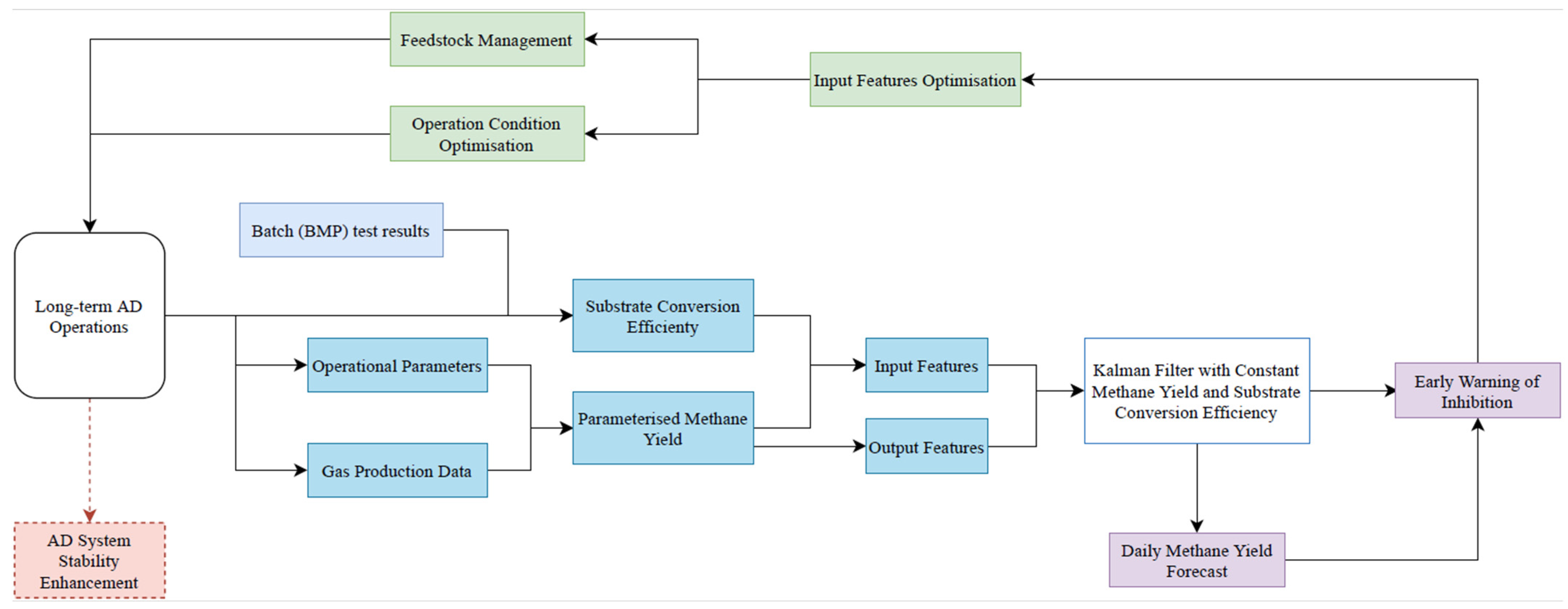
The results showed that the Kalman filter-based approaches generally outperformed the sliding-window method for steady-state methane production prediction, with the one-dimensional Kalman filter giving the best overall accuracy and the two-dimensional Kalman filter providing clearer identification of persistent abnormal deviations. Based on these findings, Figure 5 proposes a practical workflow that combines BMP results, operational parameters, and routine methane production data to support performance forecasting, early warning of instability, and optimisation of feedstock and operating conditions. This offers a simple decision support framework for AD systems where extensive process monitoring is not feasible.

Figure 5. Development of time-series analysis models predicting the performance of long-term food waste AD operation and system optimisation.

Despite these practical implications, several limitations should be acknowledged. First, the present framework was developed specifically for steady-state methane production prediction and therefore relies on assumptions of local linearity and approximately Gaussian process and observation noise in the Kalman filter implementations. These assumptions were adopted as practical approximations for relatively stable operating periods, but AD is inherently nonlinear and may become strongly non-stationary under sudden feedstock shifts, microbial community transitions, overload, or persistent inhibition. Under such conditions, the standard linear Gaussian Kalman filter used here may be less suitable than extended, unscented, or other robust filtering approaches, which can better accommodate nonlinear system dynamics and non-Gaussian disturbance behaviour. Accordingly, the present framework should not be interpreted as a full mechanistic representation of AD, but rather as a local prediction tool for comparatively stable reactor operation.

While the treatment of missing observations in the literature-derived semi-continuous datasets is also a limitation. A small number of missing values were replaced using the mean of the non-missing observations within the same dataset, which was considered acceptable for the relatively stable steady-state periods analysed here. However, mean imputation may underestimate variance and dampen short-term temporal structure, thereby obscuring local deviations that could otherwise influence prediction or inhibition forecast results. More robust time-series imputation approaches, such as interpolation, model-based imputation, or direct state-space estimation of missing values within the Kalman framework, should therefore be considered in future work.

A third limitation is the small and heterogeneous dataset used for model development and evaluation. Although the revised study included 10 paired datasets from three research groups, the cases still differed in substrate type, pretreatment or additive condition, OLR, HRT, and measurement frequency. These differences limit the transferability of the observed prediction performance across studies and mean that the reported error metrics should be interpreted as dataset-specific rather than universally representative. In particular, cases showing very low training-stage error, but larger evaluation-stage error suggest that some approaches remain sensitive to overfitting when applied to limited and study-specific observation series. The purpose of the present work was therefore not to establish a universally generalisable model for all AD systems, but to test whether simple BMP-coupled and time-series-based methods can provide useful localised prediction under constrained data conditions. Wider validation using more datasets, broader substrate types, and more diverse operating regimes will be required to better quantify uncertainty across disparate conditions and assess general applicability.

Moreover, the Shapiro–Wilk test indicated that residual normality was only partially satisfied across datasets. Most residual series from the Kalman filter approaches showed significant deviation from normality, whereas the sliding-window method met the normality criterion more often. These results suggest that the Gaussian noise assumption should be regarded as a practical approximation for implementing the standard linear Kalman filter, rather than as a strict property of all methane production time-series analysed in this study.

Finally, the inhibition forecast component of this study should be interpreted cautiously. In the present framework, potential inhibition was inferred from persistent outliers in methane production trends, rather than from direct biochemical confirmation such as VFA concentration, pH, alkalinity, or microbial data. Consequently, the flagged periods should be regarded as warning signals of abnormal or deteriorating performance, rather than definitive proof of biochemical inhibition. This distinction is especially important in datasets where methane production later recovered, suggesting temporary operational instability rather than irreversible failure. Future work should therefore combine the present time-series framework with richer process-monitoring variables in order to improve the specificity of inhibition diagnosis and distinguish more clearly between reversible fluctuation and true process inhibition.

Overall, the present study shows that BMP-informed time-series analysis can provide a practical route for steady-state AD performance monitoring when only limited routine methane data are available. However, its usefulness depends on the stability of the system, the quality and frequency of available measurements, and the extent to which the assumptions embedded in the chosen prediction method remain valid for the operating conditions of interest.

3. Materials and Methods

3.1. Data Collection and Preparation

The dataset used in this study included 10 paired experimental datasets collected from three research groups, covering different substrate and treatment conditions for food waste and cellulose-based AD systems (Table 3) [32,33,34,35]. Each dataset included results from both batch BMP tests and corresponding long-term continuous operation using the same or comparable feedstock.

Table 3. Summary of the datasets used for data collection and model evaluation.

Dataset	Research Group	Substrate or Additive	Data Acquisition Method	Notes	Source
I	Zhu	Food waste	Measured by authors	Baseline	[34]
II		Cellulose		Control substrate
III		Cellulose with 10 ppm 20 nm magnetite		Optimal additive dosage	[35]
IV		Cellulose with 100 ppm 20 nm magnetite		Potentially inhibitory dosage
V	Tampio	Food waste	Digitised from figure	Baseline	[33]
VI		Autoclaved food waste		Treated feedstock
VII	Zhang	Food waste	Digitised from figure	Baseline	[32]
VIII		Food waste with 50% optimal metal supplementation		Optimal additive dosage
IX		Food waste with 50% optimal metal supplementation plus EDDS		Optimal additive dosage
X		Zhang food waste with 100% optimal metal supplementation		Optimal additive dosage

Among these datasets, Dataset B was generated by the authors using pure cellulose as a model substrate to reduce the variability and compositional uncertainty commonly associated with food waste [34]. Datasets C and D were also based on cellulose and were included to evaluate additive effects under optimal and potentially inhibitory nano-magnetite dosages, thereby providing a more stable and controlled baseline for comparison [35]. Full details of the corresponding experimental setup are available in the original publication [34,35]. All other datasets were obtained from published studies, with data extracted from reported text, tables, or figures. Where applicable, the included studies also examined the effects of pretreatment or additive supplementation in both batch and continuous systems.

Cumulative methane production was used as the performance indicator for batch mode experiments, while daily methane production was used to describe long-term (semi-)continuous operation. All batch and continuous operation datasets used in this study were extracted from published studies that reported methane production and were standardised to “mL/g·VS” for subsequent simulations. In several literature-derived semi-continuous datasets, a limited number of observations were missing. As the long-term analysis focused on steady-state operation (Section 3.3), where methane production was expected to be comparatively stable, these missing values were calculated using the mean of the non-missing observations within the same dataset. This approach was adopted as a simple approximation for relatively stable time periods during AD operation. Additional operational and environmental variables, including temperature, substrate-to-inoculum (S/I) ratio, total batch digestion time, OLR, and HRT, were also recorded to examine their relationships with model accuracy.

3.2. Kinetic Study of Batch Tests

The first-order, modified Gompertz, logistic, and Cone models were selected to simulate the methane production process of batch experiment (Table 4). Recent reviews of BMP kinetic modelling indicate that these models are consistently among the most commonly applied options for batch AD experiments, while also noting that no single model is universally optimal across all substrates and operating conditions [43,44,45]. Moreover, they represent the main curve types relevant to the datasets analysed in this study: hydrolysis-limited behaviour (first-order) [46], sigmoidal methane accumulation with an explicit lag phase (modified Gompertz and logistic) [47,48], and more flexible non-ideal curvature through a shape factor (Cone) [48].

Table 4. Kinetic models for batch test biogas production.

Model	Equation		Parameters
First-order kinetic model	${\mathrm{G}}_{\left(\mathrm{t}\right)}={\mathrm{G}}_0[1-\mathrm{e}\mathrm{x}\mathrm{p}(-\mathrm{k}\mathrm{t}\left)\right]$	(1)	G0, k
Modified Gompertz model	${\mathrm{G}}_{(\mathrm{t})}={\mathrm{G}}_0\mathrm{e}\mathrm{x}\mathrm{p}[-\mathrm{e}\mathrm{x}\mathrm{p}({\displaystyle \frac{{\mathrm{R}}_{\mathrm{m}}\exp \left(1\right)}{{\mathrm{G}}_0}}\left(\mathsf{\lambda }-\mathrm{t}\right)+1)]$	(2)	G0, Rm, λ
Logistic model	${\mathrm{G}}_{\left(\mathrm{t}\right)}={\displaystyle \frac{{\mathrm{G}}_0}{1+\mathrm{e}\mathrm{x}\mathrm{p}(\frac{4{\mathrm{R}}_{\mathrm{m}}\left(\mathsf{\lambda }-\mathrm{t}\right)}{{\mathrm{G}}_0}+2)}}$	(3)	G0, Rm, λ
Cone model	${\mathrm{G}}_{\left(\mathrm{t}\right)}={\displaystyle \frac{{\mathrm{G}}_0}{1+{\left(\mathrm{k}\mathrm{t}\right)}^{-\mathrm{n}}}}$	(4)	G0, k, n

Notes: G_(t) is the cumulative methane yield at digestion time t (ml/g·VS); G₀ stands for the ultimate methane yield of substrate (ml/g·VS); k stands for hydrolysis rate (d⁻¹); t is the digestion time (d); R_m is the maximum methane production rate (L d⁻¹); λ stands for lag phase (d); n represents the shape factor; exp is the Euler’s number, which equals to 2.7183; N is the number of model parameters.

3.3. Model Development of Long-Term Operations

To capture the degradation dynamic of organic substrates and the production of methane, the abovementioned kinetic models were developed by fitting experimental data from batch tests. The fitted parameters included the ultimate methane production (G₀), hydrolysis rate (k), maximum gas production rate (R_m), lag phase (λ), and shape factor (n), depending on the best-fit model of each dataset.

This study focused specifically on the prediction of steady-state performance in long-term AD systems. Under steady-state operation, daily methane production is expected to fluctuate within a relatively narrow range around an underlying mean, provided that no major disturbances, feedstock shifts, or inhibition events occur [7,8]. Accordingly, the methane production rate, which is the main performance indicator considered in this study, was assumed to remain approximately constant over an extended period and is referred to hereafter as the “true” methane production rate. This simplification does not imply that AD is intrinsically linear. Rather, it reflects the assumption that, within a restricted and comparatively stable operating window, the short-term evolution of methane production can be approximated as a locally linear stochastic process for prediction purposes. In this study, steady-state operation was operationally defined as a period lasting at least one HRT, during which daily methane production remained within 10% of the stage mean under otherwise unchanged operating conditions. When this condition was satisfied, the reactor was considered to be operating at steady state. Deviations beyond this range during the subsequent period were treated as potential indicators of process disturbance and were further evaluated in Section 2.4. Potential departures from the steady-state assumption, including inhibition and sustained operational disturbances, were therefore assessed separately in the inhibition forecast analysis (Section 2.4).

Three time-series prediction approaches were examined, including the lag window method, and two Kalman filter implementations. For all approaches, the time step was aligned with the available measurement frequency or the substrate-feeding schedule in the original studies. All included long-term datasets were taken from published studies [32,33,34,35], with the simulations only targeting methane yield. For the long-term prediction framework, the following assumptions were applied:

(1) The analysed period corresponded to steady-state operation;

(2) No persistent inhibition had occurred during the training stage unless later identified through the inhibition forecast procedure;

(3) The latent daily methane production state evolved gradually over time;

(4) For the Kalman filter approaches, process noise and observation noise were treated as approximately Gaussian for practical implementation of the standard linear filter. These assumptions were adopted to provide a parsimonious and reproducible framework using the limited observations available from literature-derived datasets.

The lag method or sliding-window techniques enable localised data analysis by concentrating solely on daily methane yield, assuming VFAs were the only intermediate product utilised in methane generation. Three approaches with varying window sizes, which slide sequentially through the observations on a day-to-day basis, were employed. The smallest window size was chosen as 3 days, which corresponds to the typical biodegradation time of VFAs [39,40]. A second window of 9 days was included to represent a broader short-term memory. While a third window equivalent to the minimum HRT of each dataset was used to account for system scale retention effects. Since HRT varied among the included studies, the minimum reported HRT for each dataset was adopted as the dataset-specific window size to provide a conservative basis for comparison.

Two Kalman filter implementations were then developed. In the first Kalman filter approach, the hidden state was defined as the true daily methane production rate, Q_t (ml/g·VS):

$${\mathrm{x}}_{\mathrm{t}}=\left[{\mathrm{Q}}_{\mathrm{t}}\right]$$

(5)

while in the second Kalman filter approach, a two-dimensional hidden state was used involving both methane production and substrate conversion efficiency:

$${\mathrm{x}}_{\mathrm{t}}=\left[\begin{array}{c}{\mathrm{Q}}_{\mathrm{t}}\\ {\mathsf{\mu }}_{\mathrm{t}}\end{array}\right]$$

(6)

where ${\mathsf{\mu }}_{\mathrm{t}}$ is the substrate conversion efficiency at time t derived from BMP tests (Equation (7)), representing the fraction of the ultimate methane potential achieved during long-term operation. G₀ represents the ultimate methane yield of substrate derived from corresponding batch test.

$${\mathsf{\mu }}_{\mathrm{t}}={\displaystyle \frac{{\mathrm{G}}_0}{{\mathrm{Q}}_{\mathrm{t}}}}$$

(7)

In both approaches, the standard linear Gaussian Kalman filter was applied using state transition and observation equations (Equations (8) and (9)):

$${\mathrm{x}}_{\mathrm{t}}={\mathrm{A}\mathrm{x}}_{\mathrm{t}-1}+{\mathrm{w}}_{\mathrm{t}}$$

(8)

$${\mathrm{y}}_{\mathrm{t}}={\mathrm{H}\mathrm{x}}_{\mathrm{t}}+{\mathrm{v}}_{\mathrm{t}}$$

(9)

where $y_{\mathrm{t}}$ is the observed daily methane yield, A = [1] assumes a locally constant methane production state during steady-state operation, H = [1] maps the hidden state directly to the observation, and ${\mathrm{w}}_{\mathrm{t}}~\mathcal{N}(0,\mathrm{Q})$ and ${\mathrm{v}}_{\mathrm{t}}~\mathcal{N}(0,\mathrm{R})$ represent process and observation noise, respectively. The observation noise covariance R was estimated dynamically from the spread of the reported minimum, maximum, and average methane production values at each time step, whereas the process noise covariance Q was updated adaptively from the discrepancy between predicted and observed methane production values. Therefore, larger within-time-step variation increased R, and larger prediction mismatches increased Q. This data-driven specification was adopted to reflect variable measurement quality and modest deviations from ideal steady-state behaviour in the literature-derived datasets [49].

3.4. Model Performance Evaluation

The assessment of kinetic model performance in batch tests involved comparing predicted gas production values with corresponding experimental data. The differences were assessed using three metrics: the coefficient of determination (R²), the root mean squared error (RMSE), and Akaike information criterion (AIC).

• R², or the fitness index, helps to gauge the proportion of variance explained by the model.
• RMSE gives information about how well the predictions from a model match the measurements by calculating the average magnitude of the residuals in the model [50].
• AIC is an alternative measure that aims to balance the goodness of fit of a model and its complexity (number of parameters). It is commonly used for model selection, especially for cases involving multiple models that are nested or have different levels of complexity [51].

For long-term AD simulations, the predicted methane production values were compared with the corresponding experimental measurements in the evaluation dataset using mean absolute error (MAE), RMSE, bias, and R². MAE and RMSE were used to assess prediction error, bias was used to indicate systematic over- or underestimation, and R² was used to describe how well the observed variation pattern was reproduced [52,53,54].

For the Kalman filter approaches, the normality of residuals was assessed using the Shapiro–Wilk test on the differences between observed and predicted daily methane production values. The test statistics and corresponding p-values are provided in Supplementary Table S4.

4. Conclusions

This study developed and evaluated a practical framework for predicting steady-state methane production in long-term food waste AD by combining BMP test results with time-series analyses. Across the 10 paired datasets, the Cone model most often gave the best fit to batch methane production curves, indicating that the collected BMP profiles were generally better represented by gradual, non-ideal accumulation patterns than by strongly sigmoidal behaviour. For long-term prediction, the one-dimensional Kalman filter provided the best overall accuracy, whereas the two-dimensional Kalman filter, which incorporated substrate conversion efficiency, was less flexible but more effective at highlighting persistent abnormal deviations associated with potential inhibition. The sliding-window method provided a simple baseline. However, it was more sensitive to local fluctuations and generally less accurate.

These findings show that BMP-informed time-series analysis can support methane forecasting, noise removal, and early warning of instability using only limited routine methane production data. The framework was not intended to reproduce the full nonlinear complexity of AD, but rather to provide localised prediction under comparatively stable operating conditions. Its practical value lies in offering a simple decision support tool for systems where extensive biochemical monitoring is not feasible. Future work should expand validation across more substrates and operating regimes, incorporate richer process-monitoring variables, and test nonlinear or robust filtering approaches for more dynamic AD systems.

References

- Browne, J.D.; Murphy, J.D. Assessment of the resource associated with biomethane from food waste. Appl. Energy 2013, 104, 170–177. [Google Scholar] [CrossRef] [Scilit]
- Xu, F.; Li, Y.; Ge, X.; Yang, L.; Li, Y. Anaerobic digestion of food waste—Challenges and opportunities. Bioresour. Technol. 2018, 247, 1047–1058. [Google Scholar] [CrossRef] [Scilit]
- Arvanitoyannis, I.S.; Kassaveti, A.; Ladas, D. Waste Management for the Food Industries. In Food Science and Technology: International Series, Front Matter, Copyright, Dedication, Contributors, Preface, Abbreviations; Academic Press: Cambridge, MA, USA, 2008; pp. 345–410. [Google Scholar] [CrossRef] [Scilit]
- Traversi, D.; Bonetta, S.; Degan, R.; Villa, S.; Porfido, A.; Bellero, M.; Carraro, E.; Gilli, G. Environmental Advances Due to the Integration of Food Industries and Anaerobic Digestion for Biogas Production: Perspectives of the Italian Milk and Dairy Product Sector. Bioenergy Res. 2013, 6, 851–863. [Google Scholar] [CrossRef] [Scilit]
- Koupaie, E.H.; Leiva, M.B.; Eskicioglu, C.; Dutil, C. Mesophilic batch anaerobic co-digestion of fruit-juice industrial waste and municipal waste sludge: Process and cost-benefit analysis. Bioresour. Technol. 2014, 152, 66–73. [Google Scholar] [CrossRef] [Scilit]
- Zaks, D.P.M.; Winchester, N.; Kucharik, C.J.; Barford, C.C.; Paltsev, S.; Reilly, J.M. Contribution of anaerobic digesters to emissions mitigation and electricity generation under U.S. climate policy. Environ. Sci. Technol. 2011, 45, 6735–6742. [Google Scholar] [CrossRef] [Scilit]
- Lauwers, J.; Appels, L.; Thompson, I.P.; Degrève, J.; Van Impe, J.F.; Dewil, R. Mathematical modelling of anaerobic digestion of biomass and waste: Power and limitations. Prog. Energy Combust. Sci. 2013, 39, 383–402. [Google Scholar] [CrossRef] [Scilit]
- Donoso-Bravo, A.; Mailier, J.; Martin, C.; Rodríguez, J.; Aceves-Lara, C.A.; Wouwer, A.V. Model selection, identification and validation in anaerobic digestion: A review. Water Res. 2011, 45, 5347–5364. [Google Scholar] [CrossRef] [Scilit]
- Petre, E.; Roman, M.; Selişteanu, D. Nonlinear estimation and control schemes for a complex anaerobic digestion of microalgae with unknown kinetics and inputs. Bioresour. Technol. 2019, 287, 121429. [Google Scholar] [CrossRef] [Scilit]
- Ohemeng-Ntiamoah, J.; Datta, T. Perspectives on variabilities in biomethane potential test parameters and outcomes: A review of studies published between 2007 and 2018. Sci. Total Environ. 2019, 664, 1052–1062. [Google Scholar] [CrossRef] [Scilit]
- Holliger, C.; Alves, M.; Andrade, D.; Angelidaki, I.; Astals, S.; Baier, U.; Bougrier, C.; Buffière, P.; Carballa, M.; de Wilde, V.; et al. Towards a standardization of biomethane potential tests. Water Sci. Technol. 2016, 74, 2515–2522. [Google Scholar] [CrossRef] [Scilit]
- Liu, Y.; He, P.; Peng, W.; Zhang, H.; Lü, F. Biochemical methane potential database: A public platform. Bioresour. Technol. 2024, 393, 130111. [Google Scholar] [CrossRef] [Scilit]
- Gallert, C.; Henning, A.; Winter, J. Scale-up of anaerobic digestion of the biowaste fraction from domestic wastes. Water Res. 2003, 37, 1433–1441. [Google Scholar] [CrossRef] [Scilit]
- Morales-Polo, C.; del Mar Cledera-Castro, M.; Yolanda Moratilla Soria, B. Reviewing the anaerobic digestion of food waste: From waste generation and anaerobic process to its perspectives. Appl. Sci. 2018, 8, 1804. [Google Scholar] [CrossRef] [Scilit]
- Parker, W.J. Application of the ADM1 model to advanced anaerobic digestion. Bioresour. Technol. 2005, 96, 1832–1842. [Google Scholar] [CrossRef] [Scilit] [PubMed]
- Simeonov, I.; Hubenov, V. Application of Artificial Intelligence for Prediction, Monitoring, Optimization and Control of Anaerobic Digestion Processes—A Review. Processes 2025, 13, 3812. [Google Scholar] [CrossRef] [Scilit]
- Yang, Z.; Larsen, O.C.; Muhayodin, F.; Hu, J.; Xue, B.; Rotter, V.S. Review of anaerobic digestion models for organic solid waste treatment with a focus on the fates of C, N, and P. Energy Ecol. Environ. 2025, 10, 1–14. [Google Scholar] [CrossRef] [Scilit]
- Ge, Y.; Tao, J.; Wang, Z.; Mu, L.; Guo, W.; Cheng, Z.; Yan, B.; Shi, Y.; Su, H.; Chen, G. A hybrid approach of anaerobic digestion model no. 1 and machine learning to model and optimize continuous anaerobic digestion processes. Biomass Bioenergy 2024, 184, 107176. [Google Scholar] [CrossRef] [Scilit]
- Sbarciog, M.; Bhonsale, S.; De Buck, V.; Akkermans, S.; Polanska, M.; Van Impe, J. Modelling and Simulation of Co-digestion in Anaerobic Digestion Systems. IFAC-Pap. 2022, 55, 403–408. [Google Scholar] [CrossRef] [Scilit]
- Zhang, Y.; Yang, Z.; Xu, R.; Xiang, Y.; Jia, M.; Hu, J.; Zheng, Y.; Xiong, W.; Cao, J. Enhanced mesophilic anaerobic digestion of waste sludge with the iron nanoparticles addition and kinetic analysis. Sci. Total Environ. 2019, 683, 124–133. [Google Scholar] [CrossRef] [Scilit]
- Van der Berg, D.J.; Teke, G.M.; Johann, F.G. Predicting commercial-scale anaerobic digestion using biomethane potential. Renew. Energy 2024, 235, 121304. [Google Scholar] [CrossRef] [Scilit]
- Zhao, X.; Li, L.; Wu, D.; Xiao, T.; Ma, Y.; Peng, X. Modified Anaerobic Digestion Model No. 1 for modeling methane production from food waste in batch and semi-continuous anaerobic digestions. Bioresour. Technol. 2019, 271, 109–117. [Google Scholar] [CrossRef] [Scilit]
- Yu, L.; Wensel, P.C.; Ma, J.; Chen, S. Mathematical Modeling in Anaerobic Digestion (AD). J. Bioremed. Biodegrad. 2013, S4, 003. [Google Scholar] [CrossRef]
- Batstone, D.J.; Keller, J.; Angelidaki, I.; Kalyuzhnyi, S.V.; Pavlostathis, S.G.; Rozzi, A. The IWA Anaerobic Digestion Model No 1 (ADM1). Water Sci. Technol. 2018, 45, 65–73. [Google Scholar] [CrossRef] [Scilit]
- Batstone, D.J.; Puyol, D.; Flores-Alsina, X.; Rodríguez, J. Mathematical modelling of anaerobic digestion processes: Applications and future needs. Rev. Environ. Sci. Biotechnol. 2015, 14, 595–613. [Google Scholar] [CrossRef] [Scilit]
- Choi, S.; Kim, S.I.; Chairattanawat, C.; Hwang, S. Transformer-based multi-step time series forecasting of methane yield in full-scale anaerobic digestion. Water Res. 2025, 286, 124276. [Google Scholar] [CrossRef] [Scilit] [PubMed]
- Kalman, R.E. A New Approach to Linear Filtering and Prediction Problems. In Control Theory; John Wiley & Sons, Inc.: Hoboken, NJ, USA, 2000; pp. 167–179. [Google Scholar]
- Koç, C.K. Analysis of sliding window techniques for exponentiation. Comput. Math. Appl. 1995, 30, 17–24. [Google Scholar] [CrossRef] [Scilit]
- Raeyatdoost, N.; Bongards, M.; Bäck, T.; Wolf, C. Robust state estimation of the anaerobic digestion process for municipal organic waste using an unscented Kalman filter. J. Process Control 2022, 121, 50–59. [Google Scholar] [CrossRef] [Scilit]
- Tian, Y.; Pan, N.; Hu, M.; Wang, H.; Simeonov, I.; Kabaivanova, L.; Christov, N. Newton-Based Extremum Seeking for Dynamic Systems Using Kalman Filtering: Application to Anaerobic Digestion Process Control. Mathematics 2023, 11, 251. [Google Scholar] [CrossRef] [Scilit]
- Zhao, J.; Mili, L.; Fellow, L. A Decentralized H-Infinity Unscented Kalman Filter for Dynamic State Estimation Against Uncertainties. IEEE Trans. Smart Grid 2019, 10, 4870–4880. [Google Scholar] [CrossRef] [Scilit]
- Zhang, W.; Zhang, L.; Li, A. Enhanced anaerobic digestion of food waste by trace metal elements supplementation and reduced metals dosage by green chelating agent [S, S]-EDDS via improving metals bioavailability. Water Res. 2015, 84, 266–277. [Google Scholar] [CrossRef] [Scilit]
- Tampio, E.; Ervasti, S.; Paavola, T.; Heaven, S.; Banks, C.; Rintala, J. Anaerobic digestion of autoclaved and untreated food waste. Waste Manag. 2014, 34, 370–377. [Google Scholar] [CrossRef] [Scilit] [PubMed]
- Zhu, X.; Blanco, E.; Bhatti, M.; Borrion, A. Evaluating cellulose-based synthetic substrate as a model for food waste anaerobic digestion: Insights into system performance, microbial and metabolic response. Process Saf. Environ. Prot. 2025, 204, 108090. [Google Scholar] [CrossRef] [Scilit]
- Zhu, X.; Blanco, E.; Bhatti, M.; Borrion, A. Mitigating overload-induced stress in anaerobic digestion: Long-term performance and fate of nano magnetite additives. Water Res. 2025, 286, 124241. [Google Scholar] [CrossRef] [Scilit]
- Wang, Z.; Wang, S.; Zheng, X.; Liu, W.; Shen, Z. Integrating Kinetic Models with Physics-Informed Neural Networks (PINNs) for Predicting Methane Production from Anaerobic Co-Digestion of Enzyme-Modified Biodegradable Plastics and Food Waste Leachate. Water 2025, 17, 3411. [Google Scholar] [CrossRef] [Scilit]
- Catenacci, A.; Santus, A.; Malpei, F.; Ferretti, G. Early prediction of BMP tests: A step response method for estimating first-order model parameters. Renew. Energy 2022, 188, 184–194. [Google Scholar] [CrossRef] [Scilit]
- Ferreira, L.C.; Souza, T.S.O.; Fdz-Polanco, F.; Pérez-Elvira, S.I. Thermal steam explosion pretreatment to enhance anaerobic biodegradability of the solid fraction of pig manure. Bioresour. Technol. 2014, 152, 393–398. [Google Scholar] [CrossRef] [Scilit]
- Xu, N.; Liu, S.; Xin, F.; Zhou, J.; Jia, H.; Xu, J.; Jiang, M.; Dong, W. Biomethane production from lignocellulose: Biomass recalcitrance and its impacts on anaerobic digestion. Front. Bioeng. Biotechnol. 2019, 7, 191. [Google Scholar] [CrossRef] [Scilit]
- Zhu, X.; Blanco, E.; Bhatti, M.; Borrion, A. Promoting methanogenesis and stability in anaerobic digestion with nano magnetite under VFA-induced stress. Biofuel Res. J. 2025, 12, 2432–2450. [Google Scholar] [CrossRef] [Scilit]
- Zhu, X.; Blanco, E.; Bhatti, M.; Borrion, A. Improving anaerobic digestion process against acetate accumulation: Insights into organic loading rates and nano magnetite additions. Chem. Eng. J. 2025, 512, 162641. [Google Scholar] [CrossRef] [Scilit]
- Dewasme, L.; Sbarciog, M.; Rocha-Cózatl, E.; Haugen, F.; Wouwer, A.V. State and unknown input estimation of an anaerobic digestion reactor with experimental validation. Control Eng. Pract. 2019, 85, 280–289. [Google Scholar] [CrossRef] [Scilit]
- Welch, G.; Bishop, G.; Hill, C. An Introduction to the Kalman Filter; University of North Carolina at Chapel Hill: Chapel Hill, NC, USA, 1997; pp. 1–16. [Google Scholar]
- Potential, M.; Testing, B.M.P.; Selection, T.; Pererva, Y.; Miller, C.D.; Sims, R.C. Existing Empirical Kinetic Models in Biochemical Methane Potential (BMP) Testing, Their Selection and Numerical Solution. Water 2020, 12, 1831. [Google Scholar] [CrossRef] [Scilit]
- Zhang, H.; An, D.; Cao, Y.; Tian, Y.; He, J. Modeling the Methane Production Kinetics of Anaerobic Co-Digestion of Agricultural Wastes Using Sigmoidal Functions. Energies 2021, 14, 258. [Google Scholar] [CrossRef] [Scilit]
- Basak, S.R.; Chowdhury, S.A.; Khan, R.; Nury, A.H.; Alam, J.B.; Kabir, I. A review on the operational parameters and degradation kinetics used in anaerobic co-digestion of tannery residues. Waste Manag. Bull. 2025, 3, 271–292. [Google Scholar] [CrossRef] [Scilit]
- López, I.; Benzo, M.; Passeggi, M.; Borzacconi, L. A simple kinetic model applied to anaerobic digestion of cow manure. Environ. Technol. 2021, 42, 3451–3462. [Google Scholar] [CrossRef] [Scilit]
- Pramanik, S.K.; Suja, F.B.; Porhemmat, M.; Pramanik, B.K. Performance and kinetic model of a single-stage anaerobic digestion system operated at different successive operating stages for the treatment of food waste. Processes 2019, 7, 600. [Google Scholar] [CrossRef] [Scilit]
- da Silva, C.T.; Dias, B.M.D.A.; Araújo, R.E.; Pellini, E.L.; Laganá, A.A.M. A Practical Methodology for Real-Time Adjustment of Kalman Filter Process Noise for Lithium Battery State-of-Charge Estimation. Batteries 2024, 10, 233. [Google Scholar] [CrossRef] [Scilit]
- Wang, M.; Tang, S.X.; Tan, Z.L. Modeling in vitro gas production kinetics: Derivation of Logistic-Exponential (LE) equations and comparison of models. Anim. Feed Sci. Technol. 2011, 165, 137–150. [Google Scholar] [CrossRef] [Scilit]
- Motulsky, H.; Christopoulos, A. Fitting Models to Biological Data Using Linear and Nonlinear Regression: A Practical Guide to Curve Fitting; GraphPad Prism Software Inc.: San Diego, CA, USA, 2003; pp. 296–297. [Google Scholar]
- Wun, L.M.; Pearn, W.L. Assessing the statistical characteristics of the mean absolute error or forecasting. Int. J. Forecast. 1991, 7, 335–337. [Google Scholar] [CrossRef] [Scilit]
- Khoshvaght, H.; Ramyad, R.; Razmjou, A.; Khiadani, M. A critical review on selecting performance evaluation metrics for supervised machine learning models in wastewater quality prediction. J. Environ. Chem. Eng. 2025, 13, 119675. [Google Scholar] [CrossRef] [Scilit]
- Davydenko, A.; Goodwin, P. Assessing Point Forecast Bias Across Multiple Time Series: Measures and Visual Tools. Int. J. Stat. Probab. 2021, 10, 46–69. [Google Scholar] [CrossRef] [Scilit]
Disclaimer/Publisher’s Note: The statements, opinions and data contained in all publications are solely those of the individual author(s) and contributor(s) and not of MDPI and/or the editor(s). MDPI and/or the editor(s) disclaim responsibility for any injury to people or property resulting from any ideas, methods, instructions or products referred to in the content. |
© 2026 by the authors. Licensee MDPI, Basel, Switzerland. This article is an open access article distributed under the terms and conditions of the Creative Commons Attribution (CC BY) license.