Variational Autoencoder to Obtain High Resolution Wind Fields from Reanalysis Data

Abstract

Accurate wind flow prediction is essential for various applications, including the placement of wind turbines and a multitude of environmental assessments. Traditionally this can be achieved by using time-consuming computational fluid dynamics (CFD) simulations on reanalysis data. This study explores the performance of an autoencoder (AE) and a variational autoencoder (VAE) in approximating downscaled wind speed and direction using real-world reanalysis data and reference geo- and vegetation data. The AE model was trained for 2000 epochs and demonstrates the ability to replicate wind patterns with a mean absolute error (MAE) of approximately −0.9. However, the AE model exhibited a consistent underestimation of wind speeds and a directional shift of approximately 10 degrees compared to CFD reference simulations. The VAE model produced visually improved results, capturing complex wind flow structures more accurately than the AE model. It mainly achieves better local accuracy and a reduced variance of the results. The overall result suggests that while autoencoders can approximate wind flow patterns, challenges remain in capturing the full variability of wind speeds and directions with sufficient precision. The study highlights the importance of balancing reconstruction accuracy and latent space regularization in VAE models. Future work should focus on optimizing model architecture and training strategies to enhance accuracy, prediction reliability and generalizability across diverse wind conditions and various locations.

1. Introduction

Downscaling of local wind fields plays a crucial role in complex terrains, where topography and vegetation influence flow characteristics. In particular, forested sites exhibit heterogeneous wind and flux structures [1] that cannot be fully resolved by numerical weather prediction (NWP) models due to their limited spatial resolution and the lack of canopy representation. The Weather Research and Forecasting (WRF) model is one of the most used regional numerical weather prediction models in research and represents forests and vegetation as part of the surface through roughness parameterization without resolving forest structure in vertical [2]. This discrepancy poses a significant challenge for applications that depend on accurate local wind representations above forest canopies, such as wind resource assessment in forest areas [3] and short-term forecasting for wind turbine installation or raised up blade transport through forests, since lifting operations are weather related and need to be included in planning [4,5].

To overcome these challenges and better capture fine-scale wind variability, downscaling methods are employed, relying on statistical or dynamical approaches, each with specific advantages and limitations [6]. Statistical downscaling uses historical weather data at a given location to identify local systematic biases and establish relationships between coarse-resolution climate model outputs and local conditions. These biases, as well as linear and nonlinear patterns, are then used to derive correction functions and statistical relationships that can be applied to generate finer-scale projections and improve subsequent model forecasts. An overview of statistical downscaling methods can be found in Wilby et al. [7] and Labeurthre et al. [8]. Instead of applying corrections and statistical relationships, dynamic downscaling uses boundary conditions from global climate models to drive regional models that capture physical processes on a finer spatial scale. However, this method requires a large amount of computing time to generate high resolution wind information compared to statistical downscaling methods [6].

One method to go beyond the resolution of NWP is the use of computational fluid dynamics (CFD), which are also based on solving Navier–Stokes equations on a three-dimensional grid. These models can resolve wind fields on a spatial scale of few meters and include high resolution topography as well as heterogeneous forest resolution in vertical direction [9,10,11,12]. Depending on the choice of turbulence modeling and grid resolution, CFD simulations can be highly computationally demanding.

Recent developments in machine learning (ML) have led to an increased use of combining NWP and ML for downscaling tasks, especially in complex terrain. Ericson et al. [13] and Miralles et al. [14] improved near-surface wind prediction by downscaling coarse NWP data to high-resolution fields using deep learning methods over Switzerland. Dujardin and Lehning [15] went a step further by including measurement station data from Switzerland in their Convolutional Neural Network (CNN) to train their approach, which reduces bias and mean absolute error of the NWP model COSMO-1 at a reference validation station.

Recent studies have proposed physics-guided methods for wind and flow reconstruction [16]. These embed strong constraints in the loss function to enhance physical consistency.

While these approaches enforce physical consistency, they require a customized loss function and often additional assumptions or case-specific tuning. The present study in contrast focuses on learning physically already plausible 2d wind field representations through high fidelity CFD training data.

To reach meter-scale resolution, CNNs require high-resolution wind fields, which can be obtained from CFD simulations computed for selected reference sites using a detailed representation of the local forest to improves the accuracy of the CFD-simulation. This hybrid approach outperforms conventional ML downscaling methods in both accuracy and computational efficiency [17] and can achieve CFD-comparable resolution within seconds [18].

In this study, we investigate a downscaling approach for near-surface wind using CNNs trained on precomputed CFD simulations over a forested reference site. Our focus is on comparing the performance of autoencoders (AEs) and variational autoencoders (VAEs) for wind field downscaling. Model performance is evaluated using metrics such as mean absolute error (MAE), standard deviation (STD) and structural similarity index measure (SSIM) for wind speed and direction, as well as overall performance across all CFD simulations. The SSIM is an additional metric for the ability of the model to reproduce perceivable wind speed patterns or wind direction patterns without emphasizing the wind speed or direction error. By combining CFD simulations with CNNs, we establish a link between coarse-scale inputs, local topography, local forests and high-resolution wind fields, providing a parameterization approach analogous to statistical downscaling.

The paper is structured as follows. Section 2 describes study area, the used data and the CNN architecture. Section 3 presents the training strategy and results of the neural networks with real reanalysis data as input. Section 4 discusses the results and compares an autoencoder and two variations of variational autoencoder. Section 5 emphasizes the limitations of the current model and model training. Section 6 summarizes the main findings and outlines directions for future research.

2. Materials and Methods

To achieve the goal of a neural network for the approximation of high-resolution wind data the following inputs are necessary:

• High-resolution geographical data
• High-resolution vegetational data for the shape of the forest area as well as the tree heights
• Meteorological data from reanalysis or forecasts including the wind speed and wind direction or horizontal wind speed components u (from west to east) and v (from south to north).

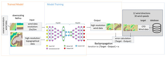
The outputs of the neural net are intended to be 2-dimensional wind speed components which are transformed to wind speed and wind direction for evaluation. To train the neural net for those outputs, a database of CFD-simulation results for a specific reference area is created. These results include wind speed components in u- and v-direction and the positional coordinates for each value. The CFD-simulation results are saved in a database and used as input for the neural network training. Figure 1 shows the approach for the trained neural network using meteorological data and high-resolution geographical data as input for the AI-model. High-resolution CFD-simulation results and high-resolution geographical data are used to train the AI-model.

Figure 1. Overview of AI training approach.

2.1. Data

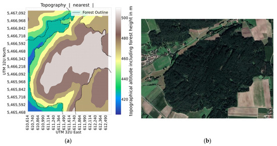
Data for training and testing the neural network comes from three sources. Geographical data (including forest data), CFD simulation data and wind from interpolated weather reanalysis data provided by Nefino (Hannover, Germany). The data is for a location near Strüth with the coordinates shown in Figure 2.

Figure 2. (a) Interpolated topographical data; (b) satellite picture.

The CFD simulation data is synthetic simulated data with a set of wind speed and direction as boundary condition. The different data sources use different grids to store their data. A common grid needs to be established and the data from the sources needs to be interpolated to this common grid to train the neural network. A grid size of 25 m was chosen. This grid can be taken from any of the sources or generated manually; in the case of this study, a new grid was generated from the coordinates included in the CFD-Data.

2.1.1. Geographical Data

For neural network, geographical data needs to include the terrain data and the shape and height of forests. The raw geographical data available only included terrain data. The shape and height of forests was then extracted from a LAZ-file. For the reference location the average tree height is 21.37 m. For the CFD-simulation-model and the neural network a constant tree height of 20 m is assumed. The raw geographical data and the forest data were used to model the CFD-simulation. To simplify the workflow for this project, the geographical data was exported from the CFD-simulation-model. The so-generated geographical data file does not discriminate between ground level and treetop.

The geographical data was imported from a .csv-file containing the values for x- and y-coordinates of the data point and the z-coordinate representing the terrain altitude over sea level. This altitude includes the height of forests.

As mentioned in Section 2.1, a fixed grid is needed as input for the neural network. To map the geographical data onto this common grid the altitude of the terrain is interpolated on this grid using the interpolation method “nearest” utilizing the “griddata” function from the scipy.interpolate library (v1.15.0). The altitudes are modified with a rescaled min–max-normalization to a scale from 0 (=a) to 1 (=b) using the following equation:

$$\mathrm{x}\prime =\mathrm{a}+(\mathrm{x}-\mathrm{m}\mathrm{i}\mathrm{n})\times (\mathrm{b}-\mathrm{a})/(\mathrm{m}\mathrm{a}\mathrm{x}-\mathrm{m}\mathrm{i}\mathrm{n})$$

(1)

x = original data

x′ = normalized data

min = minimum value

max = maximum value

a = minimum normalized value

b = maximum normalized value

The value “min” was set to 0 for the normalization of the geographical data. For the value “max” 2000 was chosen. This selection was intended to make the computation encompass the total foreseen altitude dynamic in wind park applications [19]. The region is shown as interpolated geographical data and as a satellite photo in Figure 2.

2.1.2. Wind Data from Interpolated Weather Reanalysis Data

The wind data was already interpolated onto a 25 m × 25 m grid by Nefino. It was based on wind time series from NASA’s Modern-Era Retrospective analysis for Research and Applications (MERRA-2) dataset. These are interpolated using the Virtual Wind Farm model developed from Staffel and Green [20].

Retrieving wind data for a given time and coordinate involves the following steps. First, the four closest MERRA-2 grid points are located and the u- and v-components of the wind speed at 10 m and 50 m above ground are collected. The wind speeds are then spatially interpolated to the selected coordinate by virtue of the LOESS algorithm [21].

The outlined procedure was repeatedly used to generate an hourly wind time series on a grid with a grid size of 25 m.

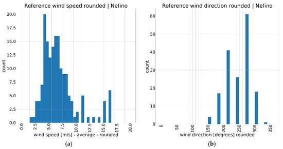
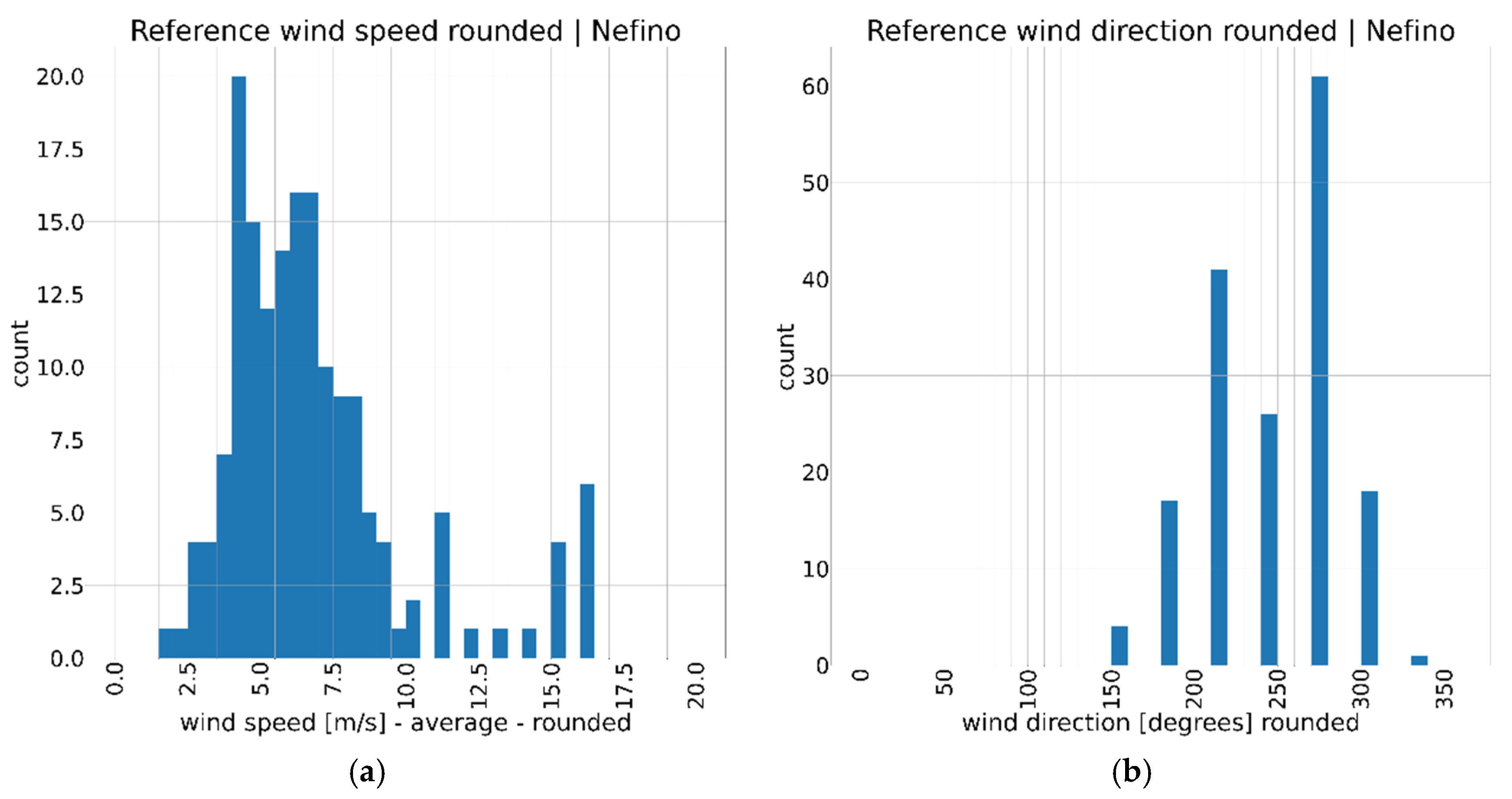
The time series contains the wind speeds u50m and v50m. Wind speed u50m refers to the wind speed in 50 m above ground from west to east. Wind speed v50m respectively describes the wind speed in 50 m above ground from south to north. As shown in Figure 3a, the wind speeds below 10 m/s follow a binomial distribution. Above 10 m/s there is little data, except for 11 m/s and 16 m/s, which are over-represented in the considered period from 23 August 2022 0:30 and 29 August 2022 23:30. There are no examples with wind speeds higher than 16 m/s. As shown in Figure 3b, the wind directions cluster around the dominant wind direction of the region. In the considered period there were no recordings of wind directions outside of 150 degrees to 330 degrees.

Figure 3. (a) Histogram of mean wind speeds in the data provided by Nefino. The mean is rounded to the next multiple of 0.5 for wind speeds below 10. For wind speeds above 10 the mean is rounded to the next multiple of 1. (b) Histogram of mean wind directions in the data provided by Nefino. The mean wind direction is further rounded to the next multiple of 30.

The centroid of this grid is included in the data in a decimal degree format. As UTM coordinates are used in the rest of the study, a recalculation of the decimal degree coordination is part of the data preprocessing. The grid is not aligned with the fixed grid mentioned in Section 2.1. Therefore, the data is aligned with the fixed grid by interpolating the wind speeds in the same way as the geographical data. This data is further modified by a min–max-normalization to a scale from −1 to 1 (see Equation (1)) with a min value of −30 and a max value of 30. Mean wind speed and mean wind direction are calculated for each time step as reference values to compare the results with a corresponding CFD-simulation.

2.1.3. CFD-Data

Reference data for training the AI-Model was generated by computational fluid dynamics (CFD) using StarCCM+ (version 2206). The simulation was built from geographical data and the average tree height. The forested area was simulated as porous medium with a Plant Area Index (PAI) to as resistance in vertical direction. This leads to higher resistance in the height of the treetop with a decreasing resistance at the trunk. As the local forest is coniferous, a PAI = 8 was used. The k-omega-SST-model in a steady-state configuration was used as turbulence model with a segregated flow solver. The computational domain consisted of approximately 4 million hexahedral cells, with a minimum cell size of 5 m near the ground and expanding to a maximum cell size of 100 m toward the top boundary. Symmetry boundary conditions were applied for the top and side walls. The atmospheric stability was assumed to be neutral, and thermal stratification as well as Coriolis force are disregarded. The evaluated area is defined by the following UTM coordinates as shown in Table 1.

Table 1. UTM-32U coordinates representing the area evaluated in the CFD-simulation.

	East	North
Coordinate 1	610,627.13	5,467,130.39
Coordinate 2	612,577.13	5,467,130.39
Coordinate 3	610,627.13	5,465,480.39
Coordinate 4	612,577.13	5,465,480.39

The inlet profile for the CFD-simulation is an atmospheric boundary layer profile with the reference speed at 37.5 m above ground. The simulation focuses on local wind speeds close to ground and the influence of forests and terrain on the wind speed with the results being considered at 37.6 m above terrain height for comparison to wind speed predictions and 50 m above terrain for comparison with reanalysis data. Only the data for wind speeds 50 m above terrain was used. The boundary conditions for the simulations are shown in the following Table 2.

Table 2. Boundary conditions for wind speed and wind direction used for the CFD-simulation. For each wind direction, every wind speed from 0.5 m/s to 20 m/s is simulated.

	Range	Step Size
Wind speed in m/s	0.5–10 m/s	0.5
Wind speed in m/s	11–20 m/s	1
Wind direction	0–330 deg	30

The CFD-data contains wind speed in x- and y-direction and the x-, y- and z-coordinates of each datapoint. As the terrain altitude for each grid square was taken from the geographical data, only the wind speeds are interpolated on the common grid in the same fashion as the geographical data and the real wind data using the “nearest” method, as explained in Section 2.1. The wind speeds in the x- and y- direction were normalized using the same values as the real wind data on a scale from −1 to 1. For easier reference, the boundary conditions of the CFD-simulation are also part of the array.

2.2. Autoencoder and Variational Autoencoder

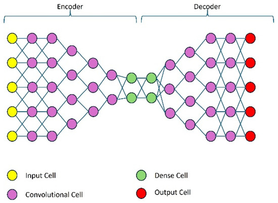
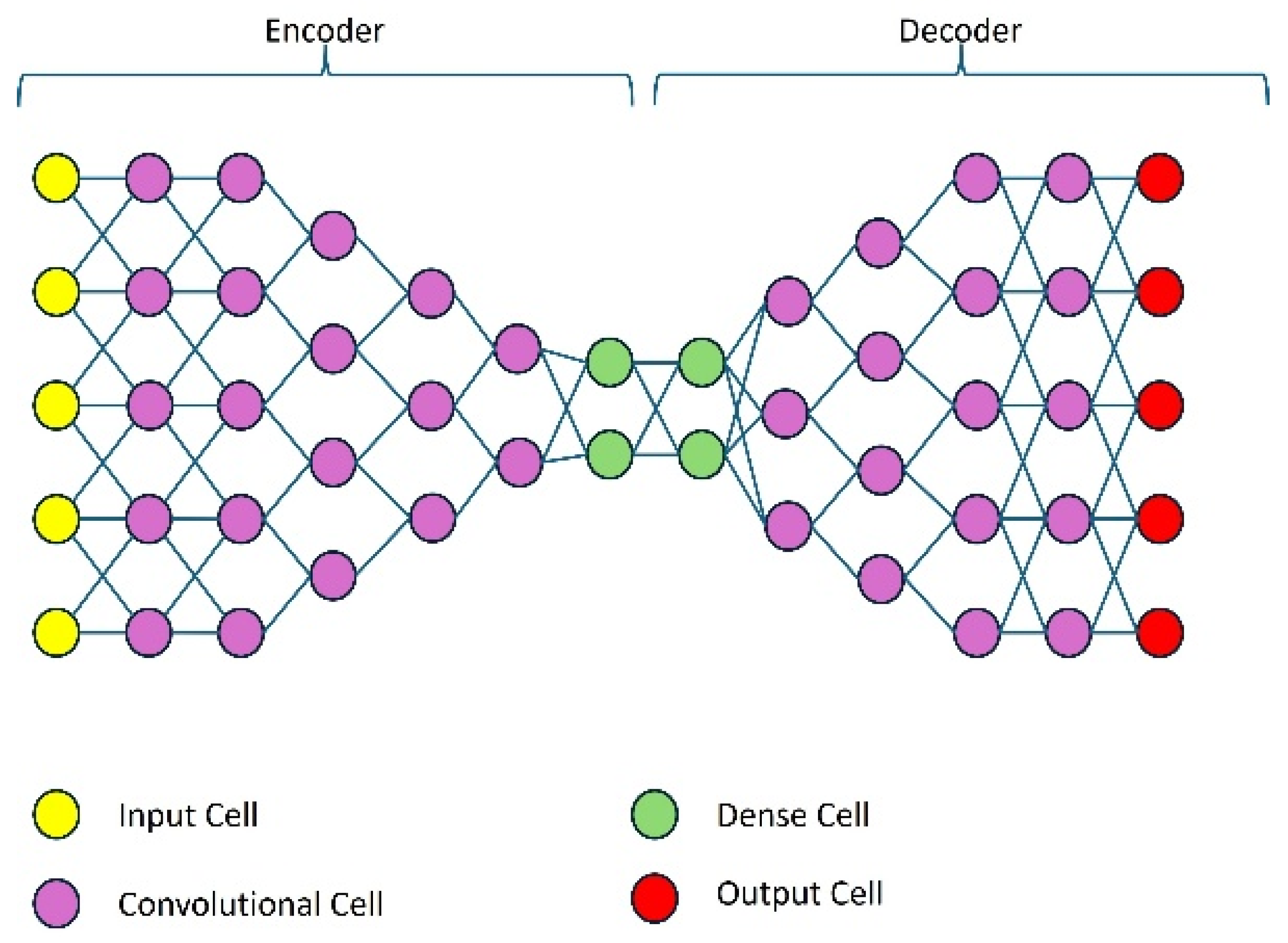
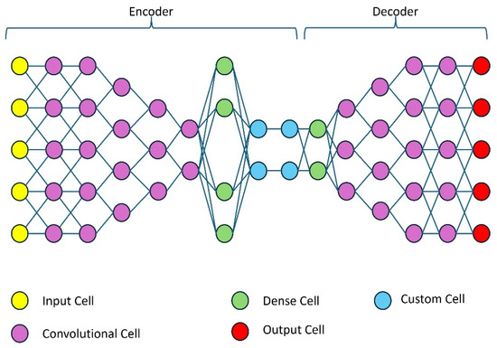
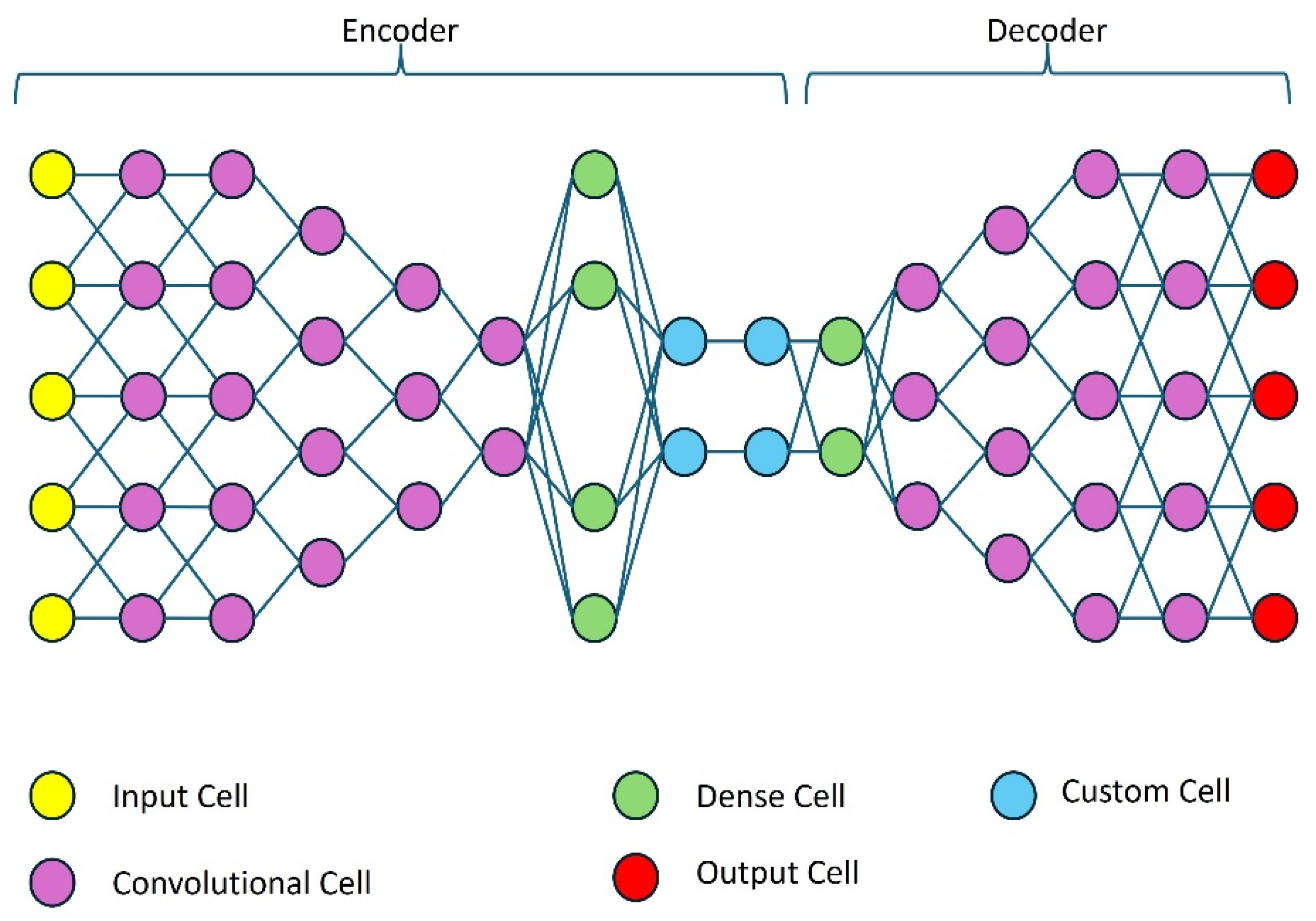
Autoencoders (AE) are a simple form of generative deep learning model able to recreate an image from a given input image [22]. The autoencoder is built from two neural networks called “encoder” and “decoder”. The encoder network takes the original multidimensional data (for example an image) and transforms it while understanding its structure. The result of the encoder is a one-dimensional vector representing the input data. The decoder is a mirror image of the encoder and reconstructs the original input from the one-dimensional vector it receives from the encoder. A problem of autoencoders is the independent encoding of each sample of the data, even if there are relationships between two samples [23] leading to the autoencoder possibly reconstructing completely different outputs from those related samples. This problem is addressed by variational autoencoders (VAEs) with the creation of a defined standard normal distribution centered around 0 to represent the data. This distribution is based on the calculation of mean and variance for each sample [23]. Figure 4 shows a representation of an autoencoder using the WINDForest Autoencoder as an example.

Figure 4. A representation of the autoencoder used in this work.

2.2.1. Autoencoder Model

The autoencoder (AE) model was built using Keras [24] and TensorFlow [25] from two Convolutional Neural Networks (CNNs) for the encoder and decoder. It is based on the code example shown in [23]. The input for the CNN is shaped as an image of the size {67,78} with three channels containing the data. The wind speed in x- and y direction is in the first 2 channels and the topographical data is given in the third channel. To keep the number of trainable parameters manageable [26], 5 convolutional 2d layers each with LeakyReLU activation are used in the encoder. These convolutional 2d layers are extracting the structural elements from the input and generate stacks of feature maps from their input. The final convolutional layer reduces the size of the feature maps down to {17,20} before a fully connected dense layer is used. The output of the encoder is realized by a dense output layer using 10 units generating a one-dimensional output vector of size of {10} for the encoder. The encoder output is the bottleneck of the AE.

The vector is then used as input for the decoder. As a first step, a dense layer transforms the input and increases its size. Following a reshape of the one-dimensional vector to a two-dimensional data of size {17,20} the data is fed through three transposed convolutional layers with LeakyReLU activation to generate the features for the final output. To arrive at an image with the same size as the input, a 4th transposed convolutional layer is paired with an Average Pooling 2d Layer. The Average Pooling operation is the followed by a LeakyReLU activation resulting in two output images. The loss-function is denoted in Equation (2):

$${\mathrm{l}\mathrm{o}\mathrm{s}\mathrm{s}}_{\mathrm{r}\mathrm{e}\mathrm{c}\mathrm{o}\mathrm{n}\mathrm{s}\mathrm{t}\mathrm{r}\mathrm{u}\mathrm{c}\mathrm{t}\mathrm{i}\mathrm{o}\mathrm{n}}={\displaystyle \frac{1}{\mathrm{n}}}\ast \sum {{(\mathrm{y}}_{\mathrm{t}\mathrm{r}\mathrm{u}\mathrm{e}}-{\mathrm{y}}_{\mathrm{p}\mathrm{r}\mathrm{e}\mathrm{d}\mathrm{i}\mathrm{c}\mathrm{t}})}^2$$

(2)

2.2.2. Variational Autoencoder

For an improved generalization ability [27], a variational autoencoder (VAE) was trained. The decoder is the same while the encoder utilizes the same configuration of convolutional 3d layers. After the convolutional layers, there are several differences (see Figure 5). First, there are two dense layers in parallel, intended to represent mean and variance from the input. The variational encoder models the approximate posterior as a diagonal Gaussian, where both the mean μ and the log-variance $\log {\sigma }^2$ are predicted by fully connected layers.

$$\mathrm{q}\left(\mathrm{z}|\mathrm{x}\right)=\mathrm{N}\left(\mathrm{\mu },\mathrm{d}\mathrm{i}\mathrm{a}\mathrm{g}\left({\mathrm{\sigma }}^2\right)\right)$$

(3)

Figure 5. Representation of the variational autoencoder used in this work.

The Kullback–Leibler divergence between the posterior and a standard normal prior $p\left(z\right)=\mathrm{{\rm N}}(0,I)$, where I denotes the $DxD$ identity matrix, is computed analytically as Equation (4) where D denotes the latent dimensionality. The KL term is weighted by a constant factor $\beta$, corresponding to a $\beta$-VAE formulation. No KL annealing or warm-up schedule is applied [28]. The total loss is the sum of the reconstruction loss and the Kullback–Leibler loss Equation (5). The variance is parameterized in log-space for numerical stability. Latent samples are obtained via reparameterization trick (Equation (6)).

$${\mathcal{L}}_{\mathrm{K}\mathrm{L}}=-{\displaystyle \frac{\mathrm{\beta }}{2}}\sum _{\mathrm{d}=1}^{\mathrm{D}}(1+\log {\mathrm{\sigma }}_{\mathrm{d}}^2-{\mathrm{\mu }}_{\mathrm{d}}^2-{\mathrm{\sigma }}_{\mathrm{e}}^2)$$

(4)

$$\mathrm{l}\mathrm{o}\mathrm{s}{\mathrm{s}}_{\mathrm{t}\mathrm{o}\mathrm{t}\mathrm{a}\mathrm{l}}=\mathrm{l}\mathrm{o}\mathrm{s}{\mathrm{s}}_{\mathrm{r}\mathrm{e}\mathrm{c}\mathrm{o}\mathrm{n}\mathrm{s}\mathrm{t}\mathrm{r}\mathrm{u}\mathrm{c}\mathrm{t}\mathrm{i}\mathrm{o}\mathrm{n}}+\mathrm{l}\mathrm{o}\mathrm{s}{\mathrm{s}}_{\mathrm{k}\mathrm{l}}$$

(5)

$$\mathrm{z}=\mathrm{\mu }+{\mathrm{e}}^{{\displaystyle \raisebox{1ex}{$\log {\mathrm{\sigma }}^2$}\!\left/ \!\raisebox{-1ex}{$2$}\right.}}\ast \mathrm{\epsilon } \mathrm{w}\mathrm{i}\mathrm{t}\mathrm{h} \mathrm{\epsilon } ~\mathrm{N}(0,\mathrm{I})$$

(6)

This adds a probabilistic component to the autoencoder enabling the model to handle data uncertainty and variability [29].

2.2.3. Training and Evaluation Method

For the training of the AE, the interpolated and normalized data from the CFD-simulations was used. The data was randomly shuffled and split. Approximately 75% of the CFD-simulations were used as training data while 25% of the CFD-simulations were used as validation data. Early tests showed little improvement beyond 2000 epochs and we used a patience of 1000 epochs to make sure to explore a significant number of epochs for every training run. The batch size of 20 was chosen. The model was only trained on the CFD-simulation dataset with wind speeds in u- and v-direction 50 m above terrain as the real wind data uses the same altitude. The model does not see any of the wind data from Section 2.1.2 at this point.

On its own, the validation loss of the model cannot be used as a reliable indicator for the quality of the model as it consists of two parts and the parameters $\mathrm{f}\mathrm{a}\mathrm{c}\mathrm{t}\mathrm{o}{\mathrm{r}}_{\mathrm{r}\mathrm{e}\mathrm{c}\mathrm{o}\mathrm{n}\mathrm{s}\mathrm{t}\mathrm{r}\mathrm{u}\mathrm{c}\mathrm{t}\mathrm{i}\mathrm{o}\mathrm{n}}$ and $facto{r}_{kl}$ have a major role in the minimum error that can be reached. The best total loss with a $\mathrm{f}\mathrm{a}\mathrm{c}\mathrm{t}\mathrm{o}{\mathrm{r}}_{\mathrm{k}\mathrm{l}}=-0.5$ is higher than 4 while a total loss below 0.8 can be achieved with a $\mathrm{f}\mathrm{a}\mathrm{c}\mathrm{t}\mathrm{o}{\mathrm{r}}_{\mathrm{k}\mathrm{l}}=-0.05$.

Hence, to evaluate the model, the mean absolute error and the standard deviation was calculated for the complete evaluated wind reanalysis dataset for the wind speed in x- and y-direction. The mean absolute error and standard deviation were also calculated for examples taken from the same dataset. In Equation (7), i and j represent the spatial grid indices of the model prediction and the interpolated CFD-data, while k indexes the individual inputs from the reanalysis dataset.

$$\mathrm{M}\mathrm{A}\mathrm{E}={\displaystyle \frac{1}{{\mathrm{N}}_{\mathrm{k}}}}\sum _{\mathrm{k}}^{{\mathrm{N}}_{\mathrm{k}}}\left({\displaystyle \frac{1}{{\mathrm{N}}_{\mathrm{i}}\ast {\mathrm{N}}_{\mathrm{j}}}}\sum _{\mathrm{i}=1}^{{\mathrm{N}}_{\mathrm{i}}}\sum _{\mathrm{j}=1}^{{\mathrm{N}}_{\mathrm{j}}}\left|{\mathrm{y}}_{\mathrm{p}\mathrm{r}\mathrm{e}\mathrm{d}\mathrm{i}\mathrm{c}\mathrm{t},(\mathrm{i},\mathrm{j})}^{\left(\mathrm{k}\right)}-{\mathrm{y}}_{\mathrm{t}\mathrm{r}\mathrm{u}\mathrm{e},(\mathrm{i},\mathrm{j})}^{\left(\mathrm{k}\right)}\right|\right)$$

(7)

$$\mathrm{S}\mathrm{T}\mathrm{D}=\sqrt{{\displaystyle \frac{1}{\mathrm{n}}}\sum _{\mathrm{i}}^{\mathrm{n}}{\mathrm{p}}_{\mathrm{i}}\ast {({\mathrm{y}}_{\mathrm{i}}-\mathrm{M}\mathrm{A}\mathrm{E})}^2}$$

(8)

For the calculation of mean absolute error and standard deviation the closest matching CFD simulation to the input data is used. The wind direction of this closest match can deviate by 15 degrees from the input. Using additional CFD-simulations at a 10° resolution, we quantify the irreducible reference error introduced by this nearest case matching. For a reference direction of 270°, CFD to CFD comparisons reveal a MAE of about 0.5–0.7 m/s for a ±10° mismatch. The error is between 0.88 and 0.99 m/s for a mismatch of ±30°. We conclude that the directional binning is not the main driver for reported errors.

As an additional metric to evaluate the similarity of an AI prediction and the closest CFD-reference, we used the Structural Similarity Index Measurement (SSIM) [30]. It expresses the perceived similarity between two images in a single number between −1 and 1 where 1 describes an identical image.

3. Results

3.1. Model Description and Training Parameters

Three model variations were examined using the same neural network layers: An autoencoder model (AE) and two variational autoencoder models (VAE1 and VAE2) were trained for 2000 epochs. The best epoch of the training in terms of error on validation data was used for evaluation. The input data for the prediction was the full real wind dataset from Nefino shown in Section 2.1.2 with 168 timesteps. Table 3 lists training specifications and training differences of the models. Training times were not recorded for those specific models. Models with a similar training scheme required about 10–15 min on an RTX 3060 graphics card. Inference was performed using Keras default batch size setting (batch size = 32) on an Intel Core i7-8565U CPU for 5 batches 100 times.

Table 3. Model training specifications.

Model	Training Length	Best Epoch	Validation Error	$\mathbf{F}\mathbf{a}\mathbf{c}\mathbf{t}\mathbf{o}{\mathbf{r}}_{\mathbf{k}\mathbf{l}}$	Inference Time in ms per Tile
AE	2000	1642	0.00677	-	5.86 ± 0.67 ms
VAE1	2000	1934	4.67443	−0.5	5.79 ± 0.57 ms
VAE2	2000	1499	0.7357	−0.05	6.22 ± 1.15 ms

The evaluation of the models was conducted with predictions of each model made on the reference inputs shown in Table 4 and the predictions for the complete input dataset. The reference inputs were chosen for their average wind speed and wind direction values being close to a reference wind speed and wind direction of a CFD-simulation.

Table 4. Wind speed and wind direction values for two reference inputs.

	Reference Input 1	Reference Input 2
Mean value	8.06 m/s 177.39 degrees	9.19 m/s 270.52 degrees
Rounded value	8 m/s 180 degrees	9 m/s 270 degrees

3.2. Evaluation of Model Variations

3.2.1. Evaluation of Model Variations on Reference Input 1

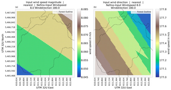
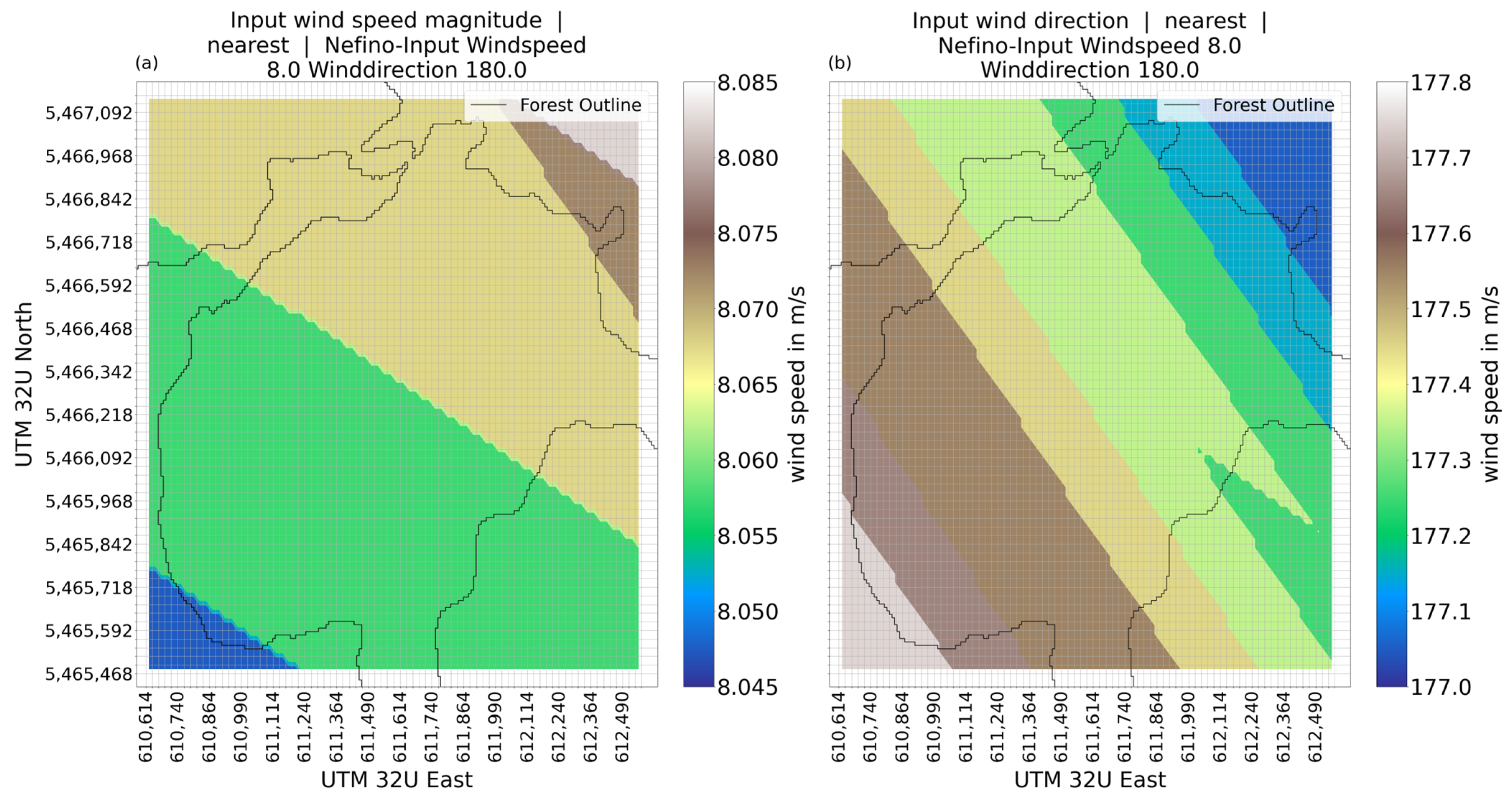
The input wind speed (Figure 6) is close to the average of 8.06 m/s with minor variations The wind direction of the input shows minor deviations of the average wind direction (177.39°) as well.

Figure 6. Wind speed magnitude (a) and wind direction (b) for reference input 1.

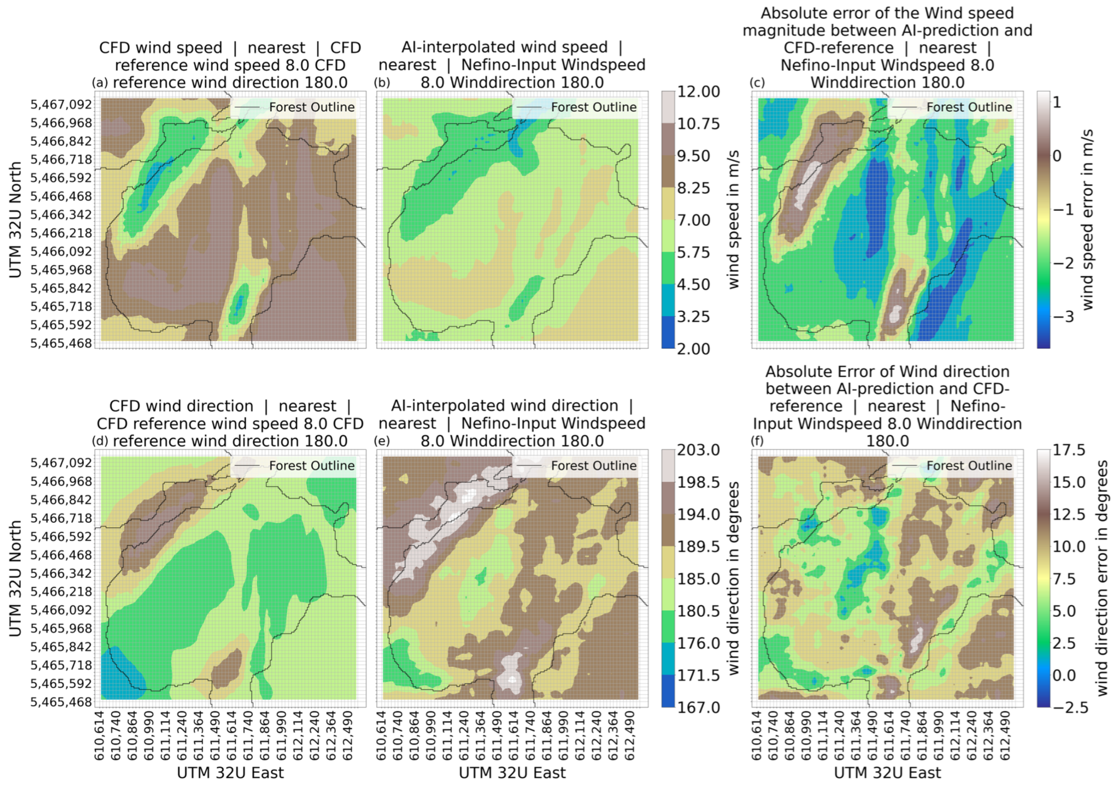
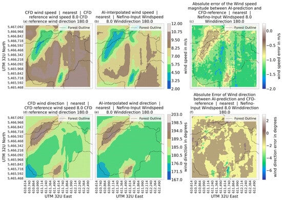
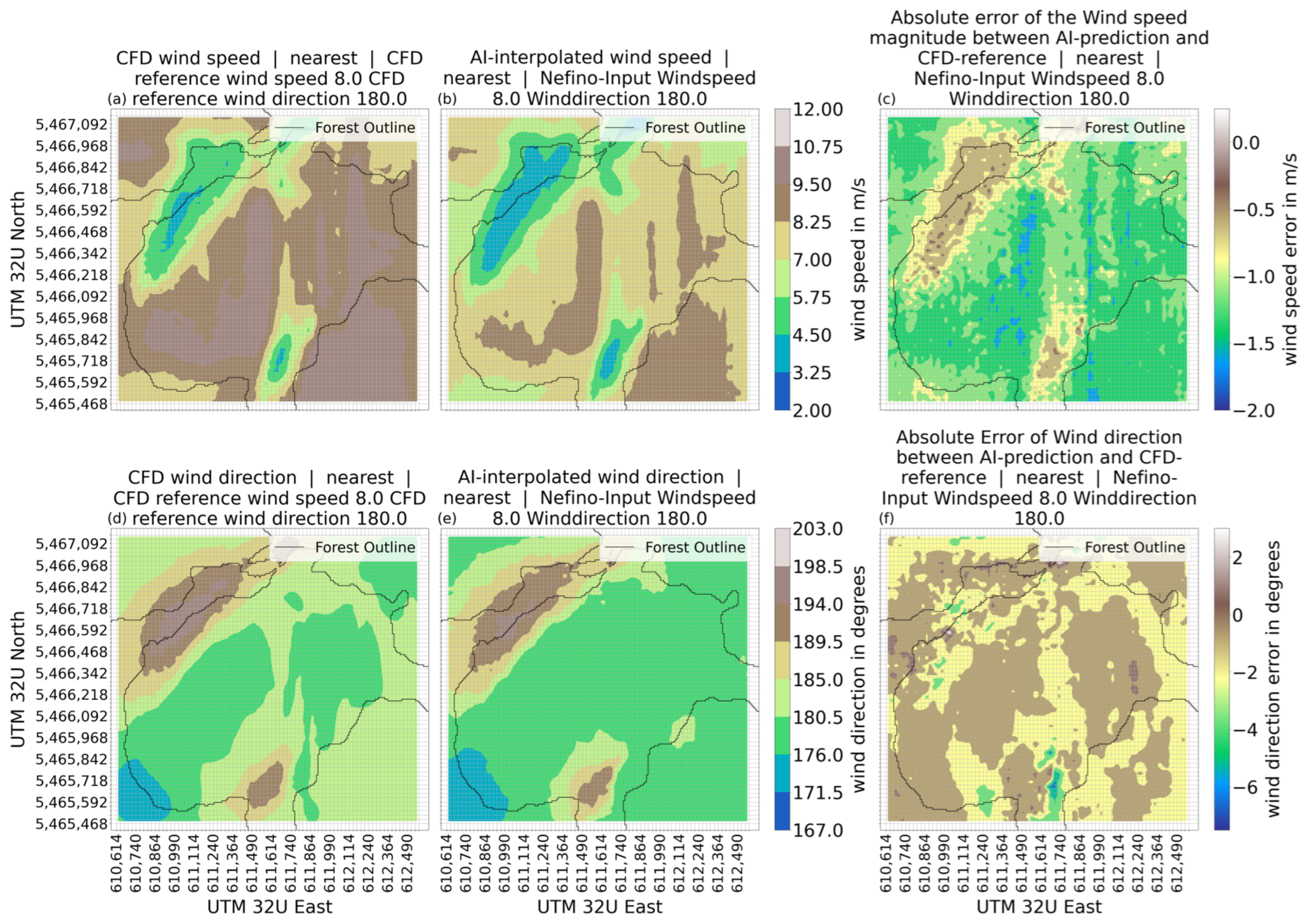
The CFD simulation shows a wide span of wind speeds from 3 m/s to 11 m/s (Figure 7a). The changes of wind speed and direction follow terrain and forest locations to some extent. In the northwest is an area where the wind speed drops to 3–5 m/s and the wind direction changes from 180 degrees to about 195 degrees. In the southwest corner of Figure 7d, a wind direction closer to 170 degrees is shown. Comparing this with the plot of the topography of Figure 2 in Section 2.1 shows the direction of the wind following the terrain at the respective altitude. At the centre of Figure 7d, the wind direction agrees with the reference wind direction being between 176° and 184°.

Figure 7. Wind speed and wind direction for the prediction made by AE-model, the CFD-reference, and the error between model prediction and CFD-reference for reference input 1; (a) wind speed CFD; (b) wind speed AE-model; (c) absolute error of wind speed between CFD and AE-model; (d) wind direction CFD; (e) wind direction AE-model; (f) absolute error of wind direction between CFD and AE-model.

The first model variation to be looked at is the AE-model. The prediction made by this model on reference input 1 shows wind directions (Figure 7e) in a similar form as the CFD-simulation. A wind direction below 180 degrees in the bottom left corner and a wind direction above 190 degrees can be seen in the top right corner. The wind direction is shifted by about +10 degrees in both corners of the area. The wind direction across the middle is shown for the CFD-reference to be around 176–185 degrees while the AE-model predicts wind direction of 185–194 degrees for large parts of the area. The error between AE-model prediction and CFD-reference is show in Figure 7f. This image verifies the shift of wind direction by +5 to 12.5 degrees for large parts. The wind speed (Figure 7b) in areas of low wind speed (i.e., at coordinates around 611,614/5,465,592) is visibly distinguishable. High wind speeds across the centre of the area are correlated, but do not visually match with the CFD simulation results as the wind speeds are significantly lower. The AE-model underestimates the wind speeds by up to 3 m/s especially in areas with high wind speeds (see Figure 7b) while overestimating low wind speeds by up to 1 m/s.

The VAE1-model is a variational autoencoder described in Section 2.2.2, with layers comparable to the AE-model. VAE-models are evaluated with the hope that this approach can improve generalization compared to the results of the autoencoder presented before. However, the generalization for multiple terrains is not tested in this work. The only addition is the implementation of a layer to calculate the Kullback–Leibler loss and a random normal distributed output of the encoder, as described in Section 2.2.3. In the first iteration, a $\mathrm{f}\mathrm{a}\mathrm{c}\mathrm{t}\mathrm{o}{\mathrm{r}}_{\mathrm{k}\mathrm{l}}$ of −0.5 was chosen (see Equation (3)).

The prediction of the VAE1-model for reference input 1 (see Table 4) shows a range of wind speeds from 12 m/s to 4 m/s (Figure 8b), agreeing well with the range of wind speeds shown in the CFD-reference (Figure 8a). The wind speeds in the northwestern valley are predicted very close to the CFD-reference at 3 to 6 m/s. In the second area of low wind speed (coordinates 611,614/5,465,592), between 3 m/s and 7 m/s was suggested by the CFD-reference, which is also predicted by the VAE-model. The wind speeds across the center of the area are predicted between 8 m/s and 12 m/s, which is close to the result of the CFD-reference. The VAE1-model shows visually discernible patterns of wind speeds that are similar to the CFD-reference. The error between VAE1-predicted wind speed and CFD-reference (Figure 8c) shows a tendency of the VAE-model to predict the wind speed too high in areas of higher wind speed. Areas of low wind speeds show a small underestimation of the wind speed.

Figure 8. Wind speed and wind direction for the prediction made by VAE1-model, the CFD-reference and the error between model prediction and CFD-reference for reference input 1; (a) wind speed CFD; (b) wind speed VAE1-model; (c) absolute error of wind speed between CFD and VAE1-model; (d) wind direction CFD; (e) wind direction VAE1-model; (f) absolute error of wind direction between CFD and VAE1-model.

The wind direction as shown in Figure 8e has a general direction of around 180 degrees with divergences in the south and northwest corresponding to the areas of lower wind speed. In the northwest, the wind direction is between 185 and 198 degrees. At the southern-central part of the area (coordinates 611,614/5,465,592) the wind direction is between 184 and 196 degrees. The southwest corner shows a spot with a wind direction between 168 to 176 degrees. These wind directions agree very close with the CFD-reference (Figure 8d). The error between the VAE1-predicted wind direction and the CFD-reference is for the large parts between −4 and −2 degrees, with two larger spots showing an error of +2 degrees in wind direction. There are some small areas showing larger errors up to −10 degrees and +6 degrees.

The training of a VAE-model is strongly influenced by the $\mathrm{f}\mathrm{a}\mathrm{c}\mathrm{t}\mathrm{o}{\mathrm{r}}_{\mathrm{k}\mathrm{l}}$ (see Equation (3)) and is changed in the following model to reduce the influence of the Kullback–Leibler loss on the training of the VAE-model. This is intended to reduce to the reconstruction error while preserving the probabilistic capability of the VAE.

To improve the reconstruction of the output, a lower $\mathrm{f}\mathrm{a}\mathrm{c}\mathrm{t}\mathrm{o}{\mathrm{r}}_{\mathrm{k}\mathrm{l}}$ of −0.05 was used to train the VAE2-model, which otherwise is the same as the VAE1-model.

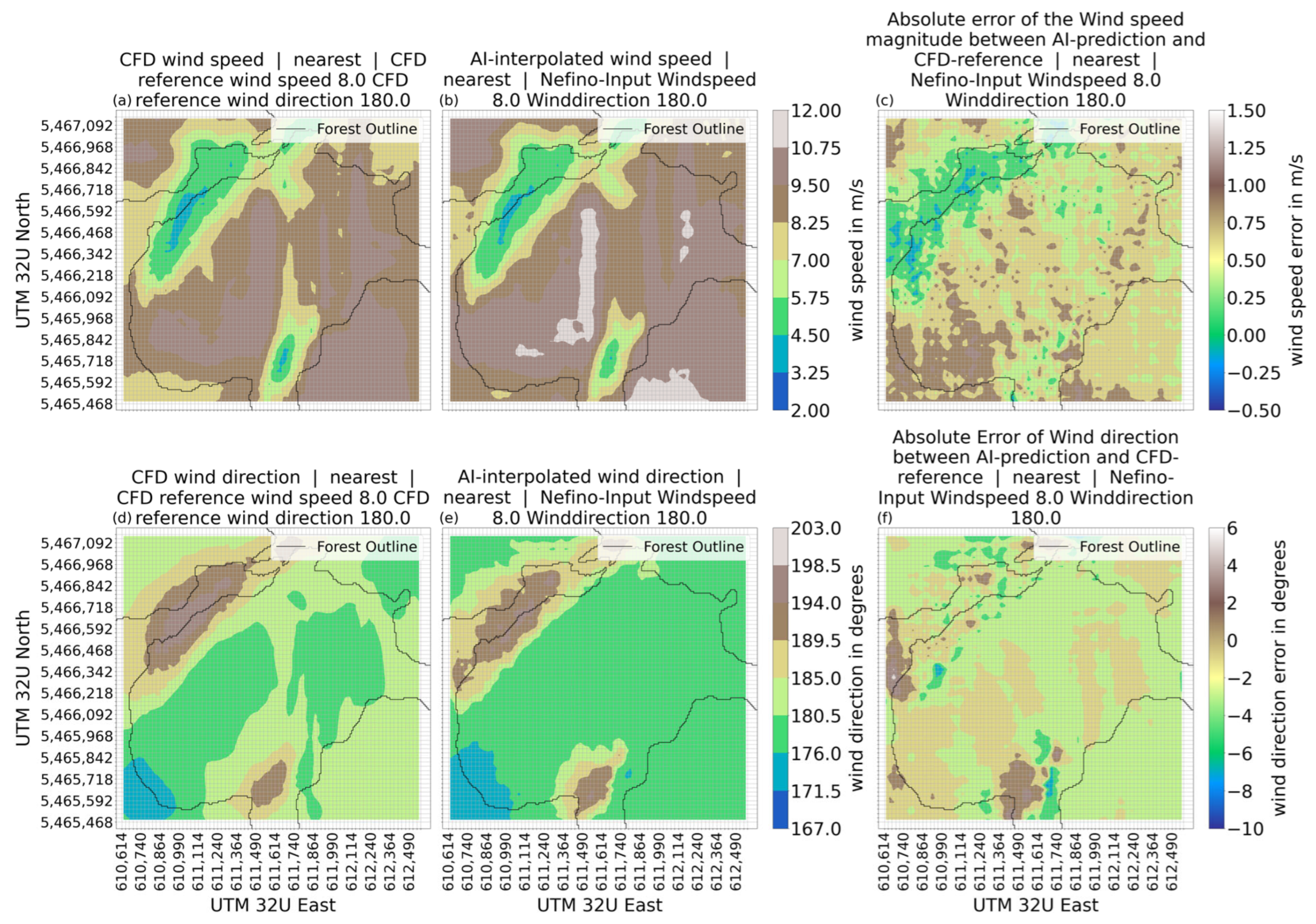
The reference input 1 results are shown in Figure 9b with a wind speed range of 3.25 m/s to 9.5 m/s. The general areas seem to be reproduced in comparison to the CFD-reference (Figure 9a), albeit with a generally lower wind speed (see Figure 9c).

Figure 9. Wind speed and wind direction for the prediction made by VAE2-model, the CFD-reference and the error between model prediction and CFD-reference for reference input 1; (a) wind speed CFD; (b) wind speed VAE2-model; (c) absolute error of wind speed between CFD and VAE2-model; (d) wind direction CFD; (e) wind direction VAE2-model; (f) absolute error of wind direction between CFD and VAE2-model.

The area of low wind speed in the northwestern corner of the area is a close representation of the CFD-reference in that area with closely matching wind speeds. However, the VAE2 result is still showing a larger area of 3.25–4.5 m/s wind speed than the CFD-reference suggests. A second small area with very closely matching wind speeds is the second area of low wind speed at coordinates 611,614/5,465,717. For most of the region, the prediction of the VAE2-model is between 1 and 1.5 m/s lower than suggested by the CFD-reference.

The wind directions predicted by the VAE2-model (Figure 9e) is a close fit to the CFD-reference (Figure 9d) with only small deviations with the structures being visibly reproduced. The error of the VAE2-model wind directions is very small, with most of the region seeing and wind direction error of 0.5 to −3 degrees. Only small spots show an error larger than −4 degrees.

To further analyze the results of the AI prediction compared to the CFD-simulation the error of the wind speed in x- and y-direction was calculated for every datapoint of the example. The mean absolute error and standard deviation were also calculated and are shown in histograms.

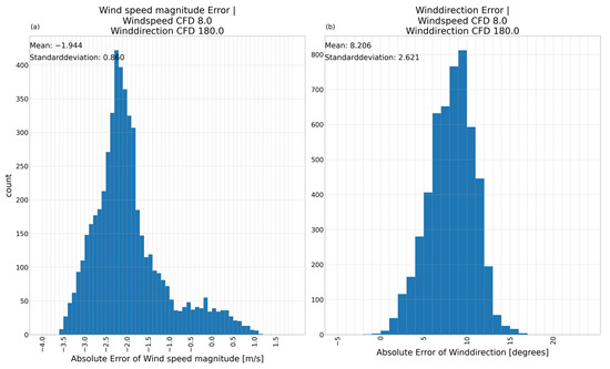
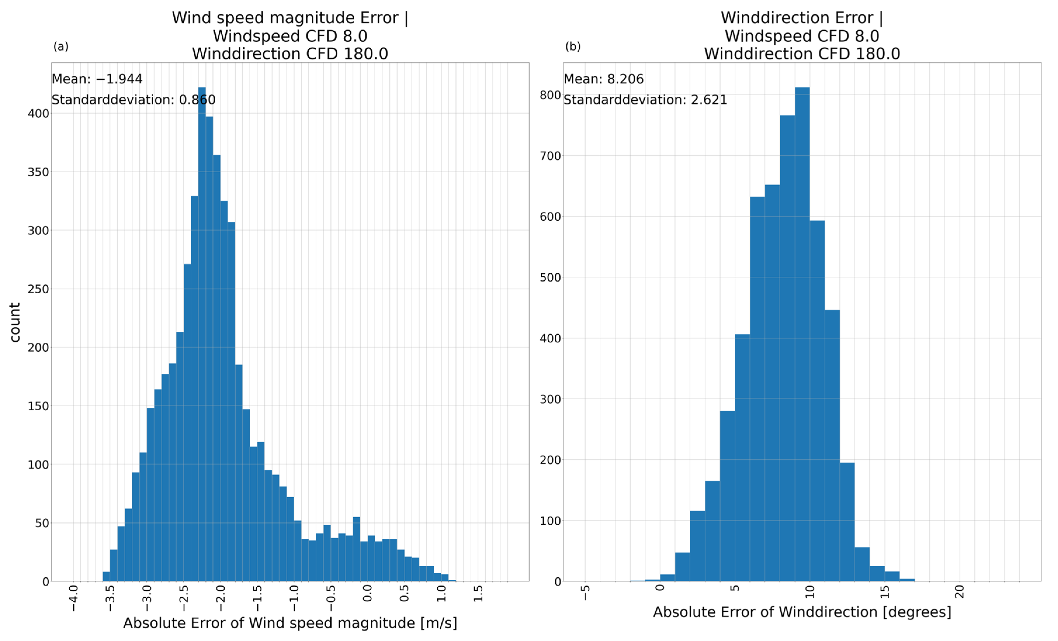
The histogram in Figure 10a shows the wind speed magnitude of the AE-model prediction matching the CFD-simulation with a mean error of −1.944 and a standard deviation of 0.860. It has multiple peaks with a main peak at −2.2 and a second much lower peak at −0.6. It shows the underestimation of the wind speed in the main wind direction for most of the area. The error of the wind direction has a mean of 8.206 and standard deviation of 2.621 (Figure 10b). These results indicate feasibility rather than best achievable accuracy. The bias of the mean is expected to be reduced with more data, but if a significant bias persists in future models, we would correct for it using postprocessing to improve the model accuracy.

Figure 10. Absolute error histogram between AE-model prediction and CFD-simulation including mean error and standard deviation. (a) Absolute error of the wind speed magnitude; (b) absolute error of the wind direction. Reference input 1.

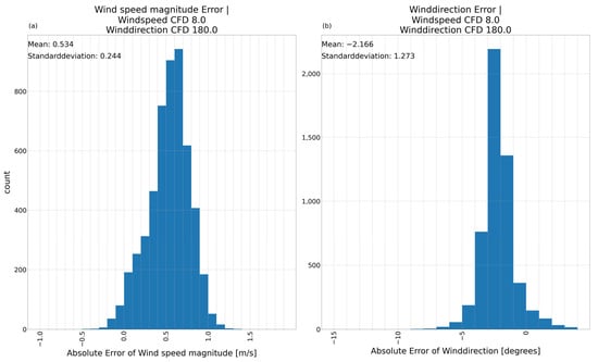
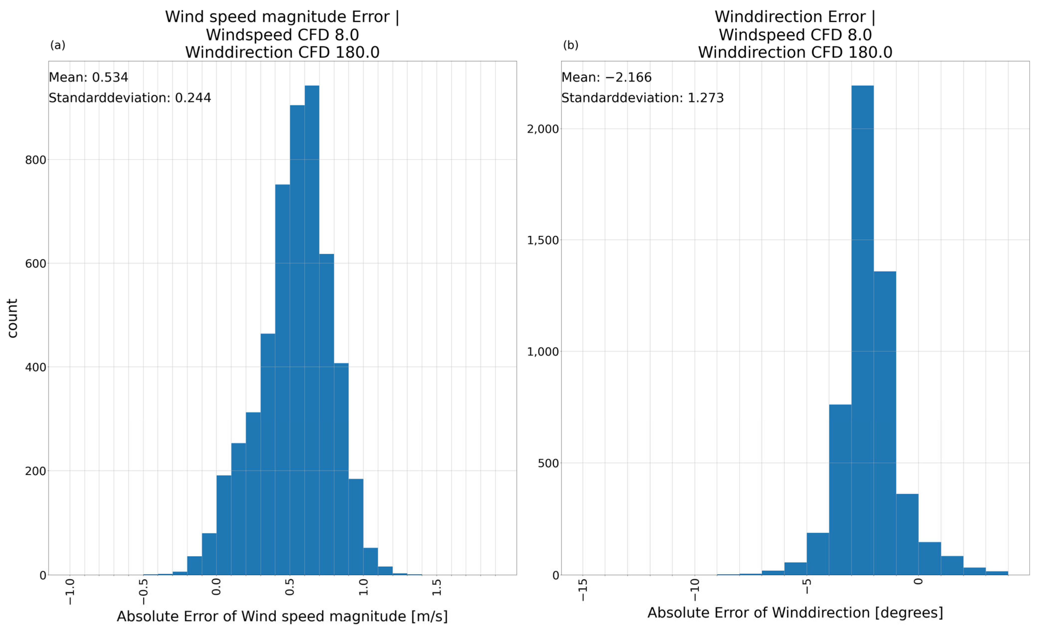
The histograms of the absolute error between VAE1-model prediction and CFD-simulation show a mean absolute error of 0.534 for the wind speed magnitude with a standard deviation of 0.244 (Figure 11a). The wind direction has a small mean of just −2.166 with a very small standard deviation of 1.273 (Figure 11b). This emphasizes the VAE1-model being a close fit to the CFD-reference for this example.

Figure 11. Absolute error histogram between VAE1-model prediction and CFD-simulation including mean error and standard deviation. (a) Absolute error of the wind speed magnitude; (b) absolute error of the wind direction. Reference input 1.

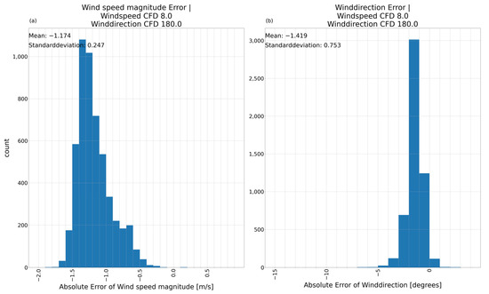
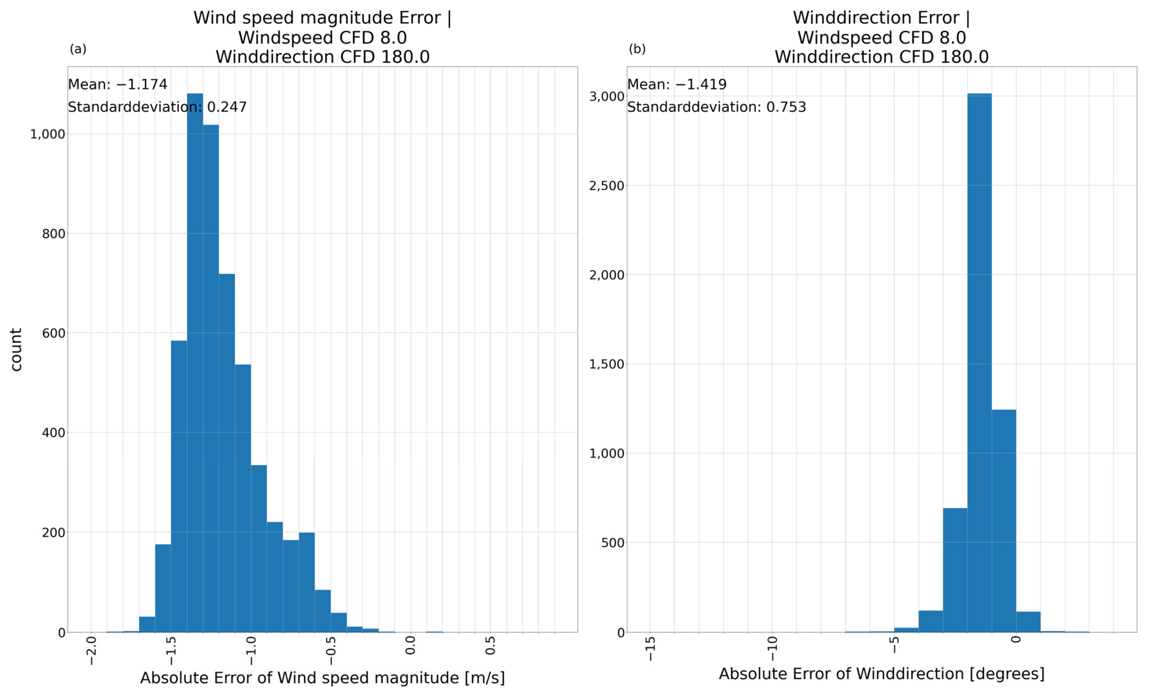
The VAE2-model results in a mean absolute error of the wind speed magnitude (Figure 12a) of −1.174 and a standard deviation of 0.247 are promising. The error between prediction and CFD-model result for the wind direction (Figure 12b) displays a mean of −1.419 and a standard deviation of 0.753. This verifies the tendency of the VAE2-model to underestimate the wind speeds. The low error of the wind direction shows the ability of the model, to keep the x- and y-component of the wind speed in balance. If future studies with a larger dataset show a remaining negative bias for the wind speed, it might be viable to correct for it using postprocessing.

Figure 12. Absolute error histogram between VAE2-model prediction and CFD-simulation including mean error and standard deviation. (a) Absolute error of the wind speed magnitude; (b) absolute error of the wind direction. Reference input 1.

To evaluate the similarity of two images besides a visual inspection the Structural Similarity Index Measurement (SSIM) is used (Table 5). The CFD-reference is compared to the predictions of the three models. The AE-model prediction for this reference input does not match the CFD-reference perfectly. Even though the wind speed magnitude is matched quite well with an SSIM of 0.92, the prediction of the wind direction falls short with only SSIM of 0.70. The VAE1-model improves on this basis, reproducing the structure of the wind speed magnitude nearly perfectly while improving on in the wind direction by close to 30%. VAE2-model matches the structures in the CFD-reference best by keeping an excellent match for the wind speed magnitude and further improving on the reproduction of the wind direction.

Table 5. Structural Similarity Index comparing the prediction of each model with the CFD-reference for reference input 1.

Model	SSIM Wind Speed	SSIM Wind Direction
AE	0.92	0.70
VAE1	0.99	0.92
VAE2	0.98	0.96

3.2.2. Evaluation of Model Variations on Reference Input 2

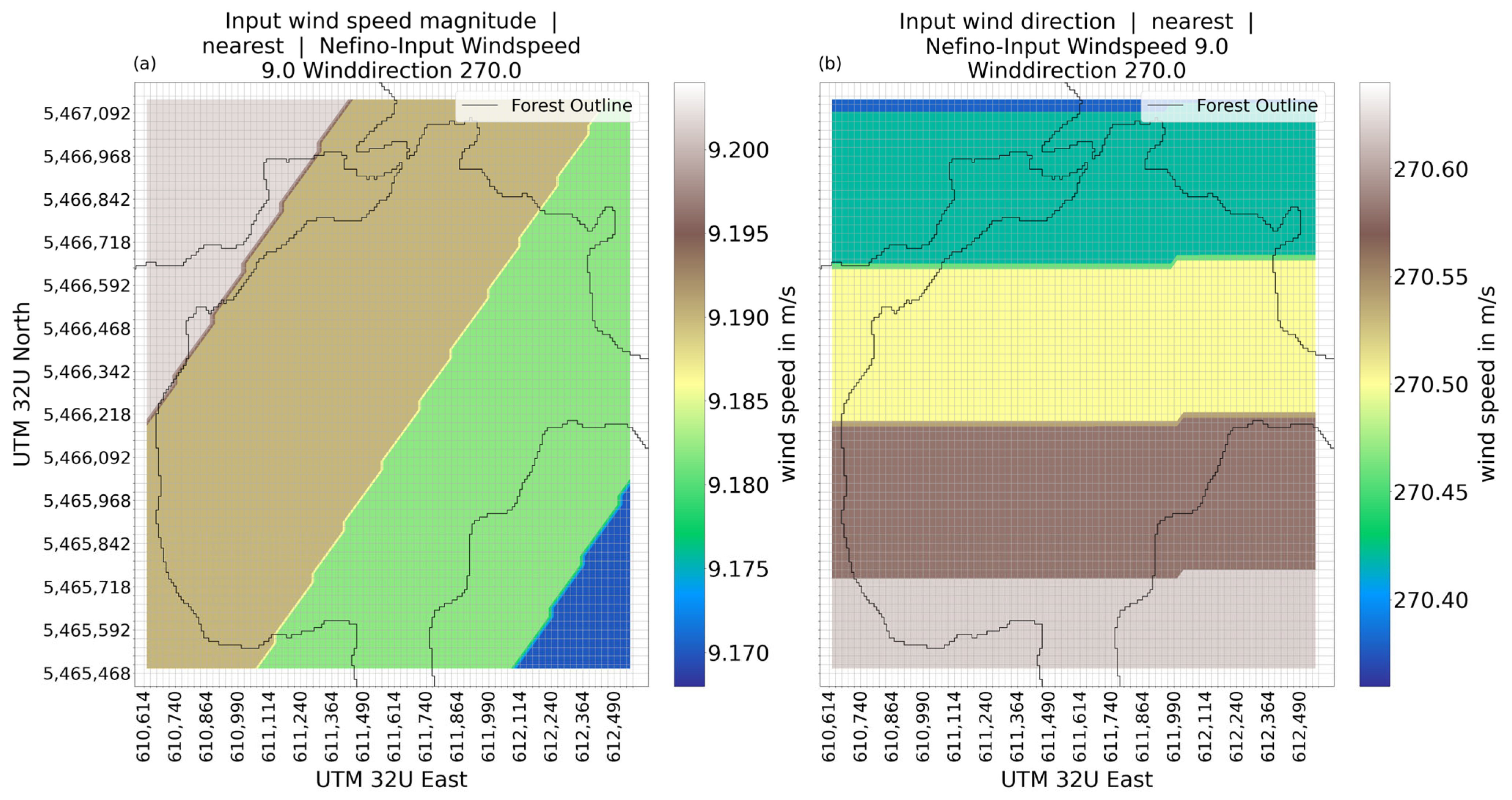
The input wind speed (Figure 13a) for reference input 2 (see Table 4) is close to the average of 9.19 m/s with minor variations The wind direction of the input shows minor deviations of the average wind direction (270.52°) as well.

Figure 13. Wind speed magnitude (a) and wind direction (b) for reference input 2.

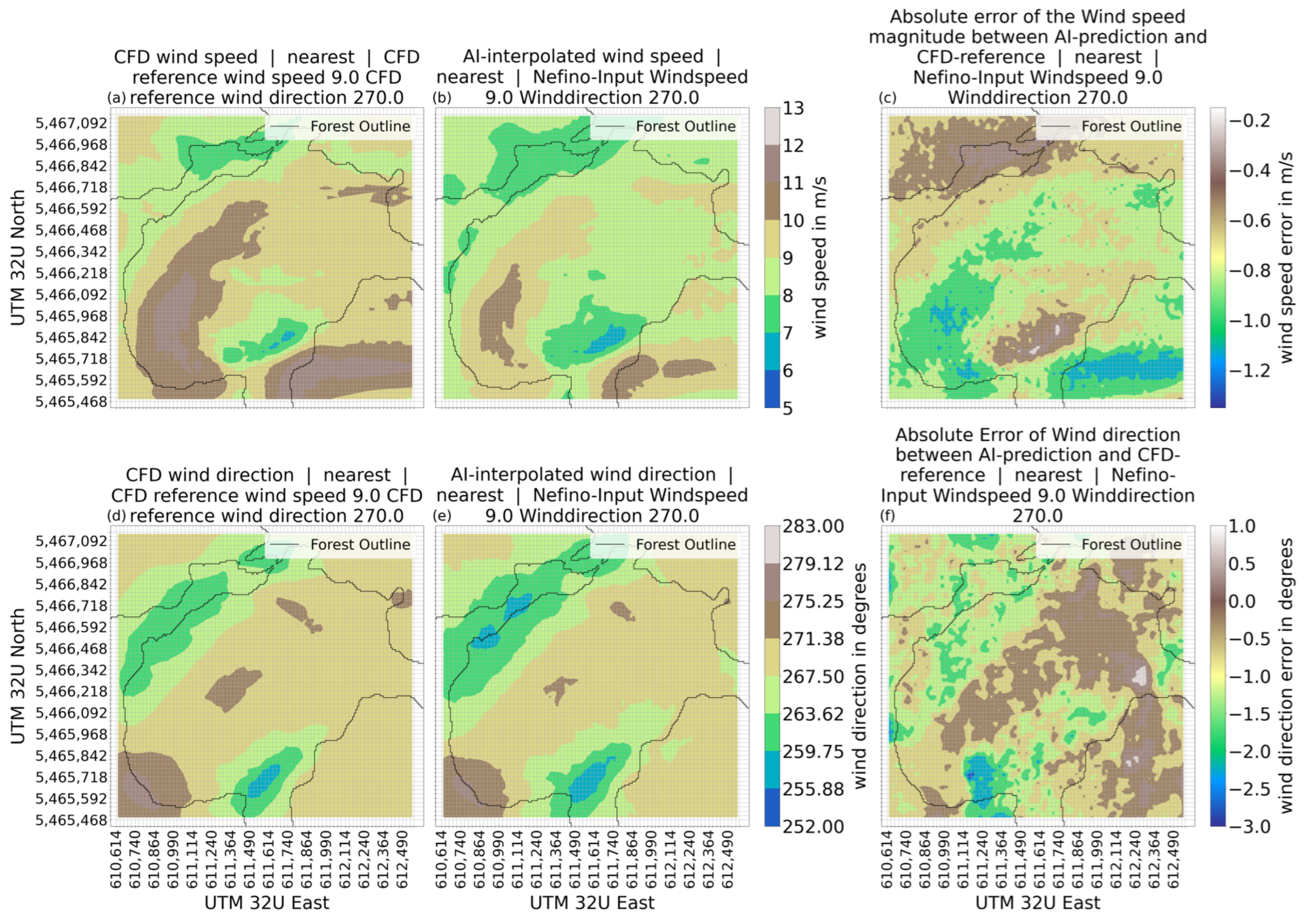
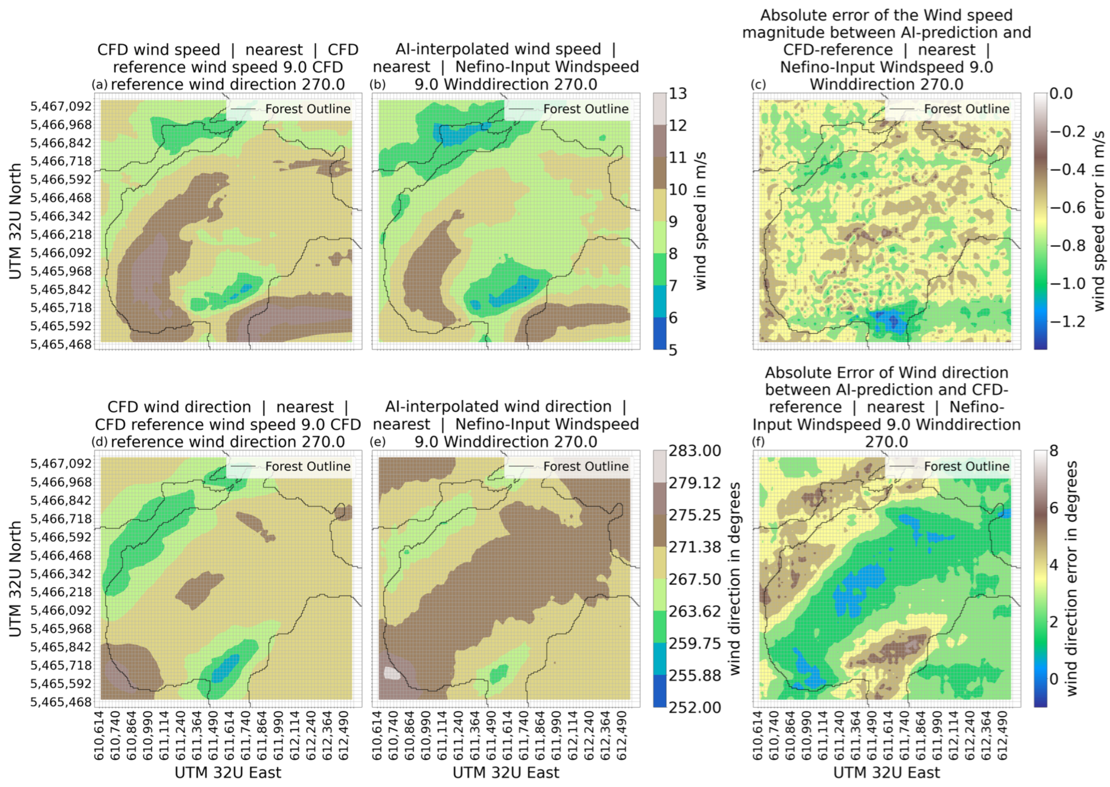
For this second reference input the AE-model produces a close approximation of the CFD-reference (Figure 14). The wind speed visually matches for the most part. Zones of high wind speed are clearly visible in the approximation made by the model. The wind speed is slightly lower for the many areas through. This is also shown in the depiction of the error (Figure 14c). The error is around −1 m/s for the central area, approaching −1.2 m/s in the areas depicting the highest wind speed in the CFD-reference. Areas of lower wind speed have a smaller error as seen in the northern part and in the area around the coordinates 611,614/5,465,592. The prediction of the wind direction made by the AE-model shows a similarly close approximation to the CFD-reference. The areas with a wind direction of 250–265 degrees are reproduced in a recognizable way while the wind direction across the centre of the area shows the expected value of about 270 degrees. This is further reinforced by the absolute error of the wind direction which is between 1 and −3 degrees and showing a large area to the east having an error of about 0 degrees.

Figure 14. Wind speed and wind direction for the prediction made by AE-model, the CFD-reference and the error between model prediction and CFD-reference for reference input 2; (a) wind speed CFD; (b) wind speed AE-model; (c) absolute error of wind speed between CFD and AE-model; (d) wind direction CFD; (e) wind direction AE-model; (f) absolute error of wind direction between CFD and AE-model.

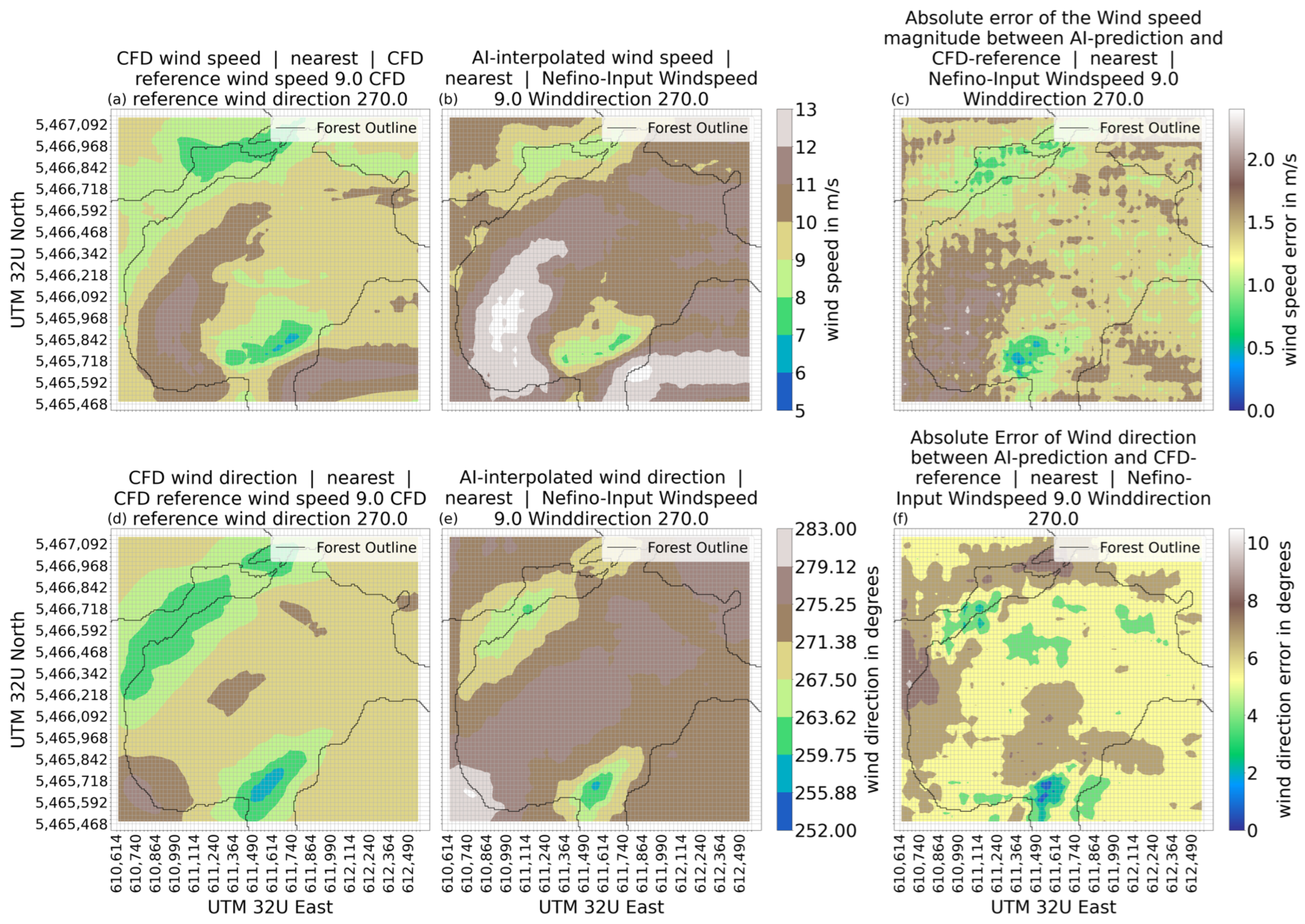
The prediction of the VAE1-model for reference input 2 shows a range of wind speeds from more than 13 m/s to 5 m/s (Figure 15b) agreeing well with the range of wind speeds shown in the CFD-reference (Figure 15a). The wind speeds in the northwestern valley are predicted as faster than the CFD-reference suggests at 8 to 9 m/s. In the second area of low wind speed (coordinates 611,614/5,465,592), between 5 m/s and 8 m/s is suggested by the CFD-reference, which the VAE1-model predicts as 7 to 9 m/s. The wind speeds across the center of the area are predicted between 10 m/s and 12 m/s, which is faster than the result of the CFD-reference. The VAE1-model shows visually discernible patterns of wind speeds that are like the CFD-reference. The error between VAE1-predicted wind speed and CFD-reference (Figure 15c) shows a tendency of the VAE-model to predict the wind speed too high in areas of higher wind speed. Areas of low wind speeds show a small underestimation of the wind speed.

Figure 15. Wind speed and wind direction for the prediction made by VAE1-model, the CFD-reference and the error between model prediction and CFD-reference for reference input 2; (a) wind speed CFD; (b) wind speed VAE1-model; (c) absolute error of wind speed between CFD and VAE1-model; (d) wind direction CFD; (e) wind direction VAE1-model; (f) absolute error of wind direction between CFD and VAE1-model.

The wind direction as shown in Figure 15e has a general direction of between 271 and 279 degrees with divergences in the south and northwest corresponding to the valleys influencing wind speed and direction. In the northwest, the wind direction is between 259 and 271 degrees. At the southern-central part of the area (coordinates 611,614/5,465,592), the wind direction is between 255 and 271 degrees. The southwest corner shows a spot with a wind direction between 279 to 283 degrees. Those wind directions generally match the structures of the CFD-reference (Figure 15d) but are generally higher than the CFD-reference suggests. The error between the VAE1-predicted wind direction and the CFD-reference is for the large parts between 4 and 6 degrees, with two larger spots showing an error of +8 degrees in wind direction.

The results of VAE2-model using reference input 2 are shown in Figure 16. The wind speed has range of 5 m/s to 11 m/s. The general areas seem to be reproduced in comparison to the CFD-reference (Figure 16a), albeit with a generally lower wind speed (see Figure 16).

Figure 16. Wind speed and wind direction for the prediction made by VAE2-model, the CFD-reference and the error between model prediction and CFD-reference for reference input 2; (a) wind speed CFD; (b) wind speed VAE2-model; (c) absolute error of wind speed between CFD and VAE2-model; (d) wind direction CFD; (e) wind direction VAE2-model; (f) absolute error of wind direction between CFD and VAE2-model.

The area of low wind speed in the northwestern corner of the area is a close representation of the CFD-reference in that area with closely matching wind speeds. However, the VAE2 result is still showing a larger area with 7–8 m/s wind speed than the CFD-reference suggests. A second small area with very closely matching wind speeds is the second area of low wind speed at coordinates 611,614/5,465,717. For most of the region, the prediction of the VAE2-model is between 0.5 and 1.0 m/s, lower than suggested by the CFD-reference.

The wind directions predicted by the VAE2-model Figure 16e is a close fit to the CFD-reference (Figure 16d) with only small deviations with the structures being visibly reproduced. The error of the VAE-2 model wind directions shows a large part of the region seeing and wind direction error of 0 to 4 degrees. In the northwestern valley and around the coordinates 611,614/5,465,717, a slightly higher wind direction error is recorded with 4–8 degrees.

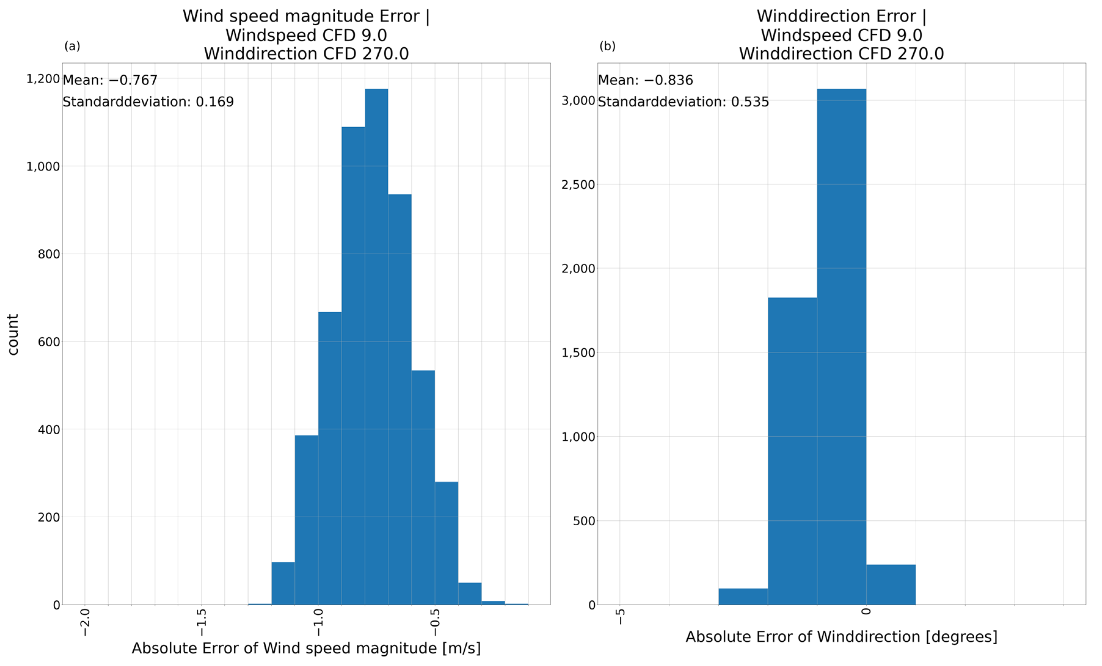
The histogram (AE) of the absolute error for reference input 2 (Figure 17) shows a different behavior than reference input 1 (Figure 10). The mean absolute error for the wind speed is −0.767 with a standard deviation of 0.169. This further supports the examination of the AE-model results with a negatively biased wind speed. For the wind direction, the mean absolute error is −0.836 with a standard deviation of 0.535. The result for reference input 2 is significantly better than for reference input 1. The model most likely did not learn all wind directions equally well, which is also supported by findings in Section 3.2.3.

Figure 17. Absolute error histogram between AE-model prediction and CFD-simulation for reference input 2 including mean error and standard deviation. (a) Absolute error of the wind speed magnitude; (b) absolute error of the wind direction. Reference input 2.

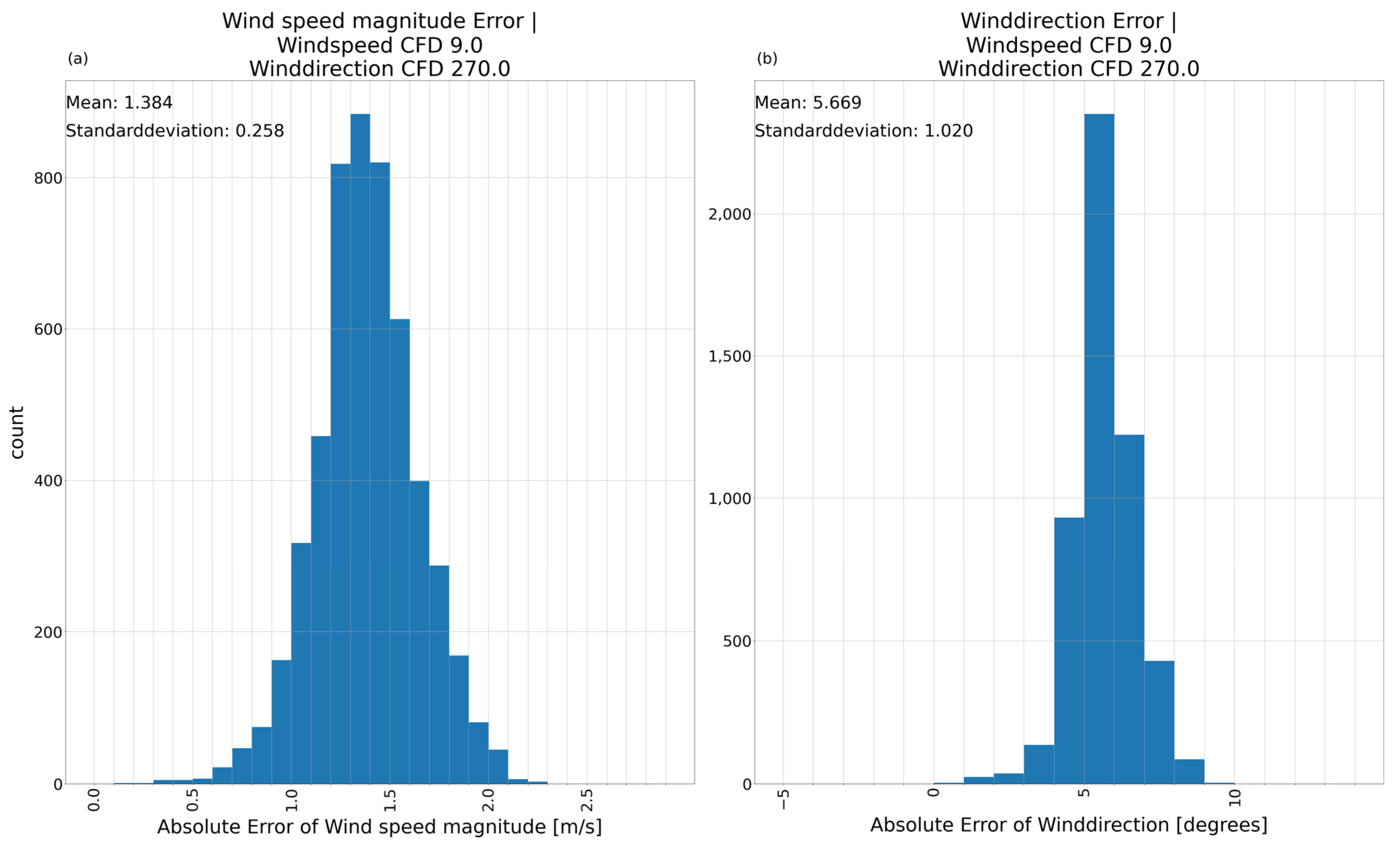
The mean absolute error (VAE1) for reference input 2 in Figure 18 is 1.384, with a standard deviation of about 0.258 for the wind speed, showing clearly the overestimation of wind speeds by this model. The wind direction has a mean absolute error of 5.669 with a standard deviation of 1.020. The mean absolute error shows a measurable difference between different inputs when comparing it to Figure 11.

Figure 18. Absolute error histogram between VAE1-model prediction and CFD-simulation for reference input 2 including mean error and standard deviation. (a) Absolute error of the wind speed magnitude; (b) absolute error of the wind direction. Reference input 2.

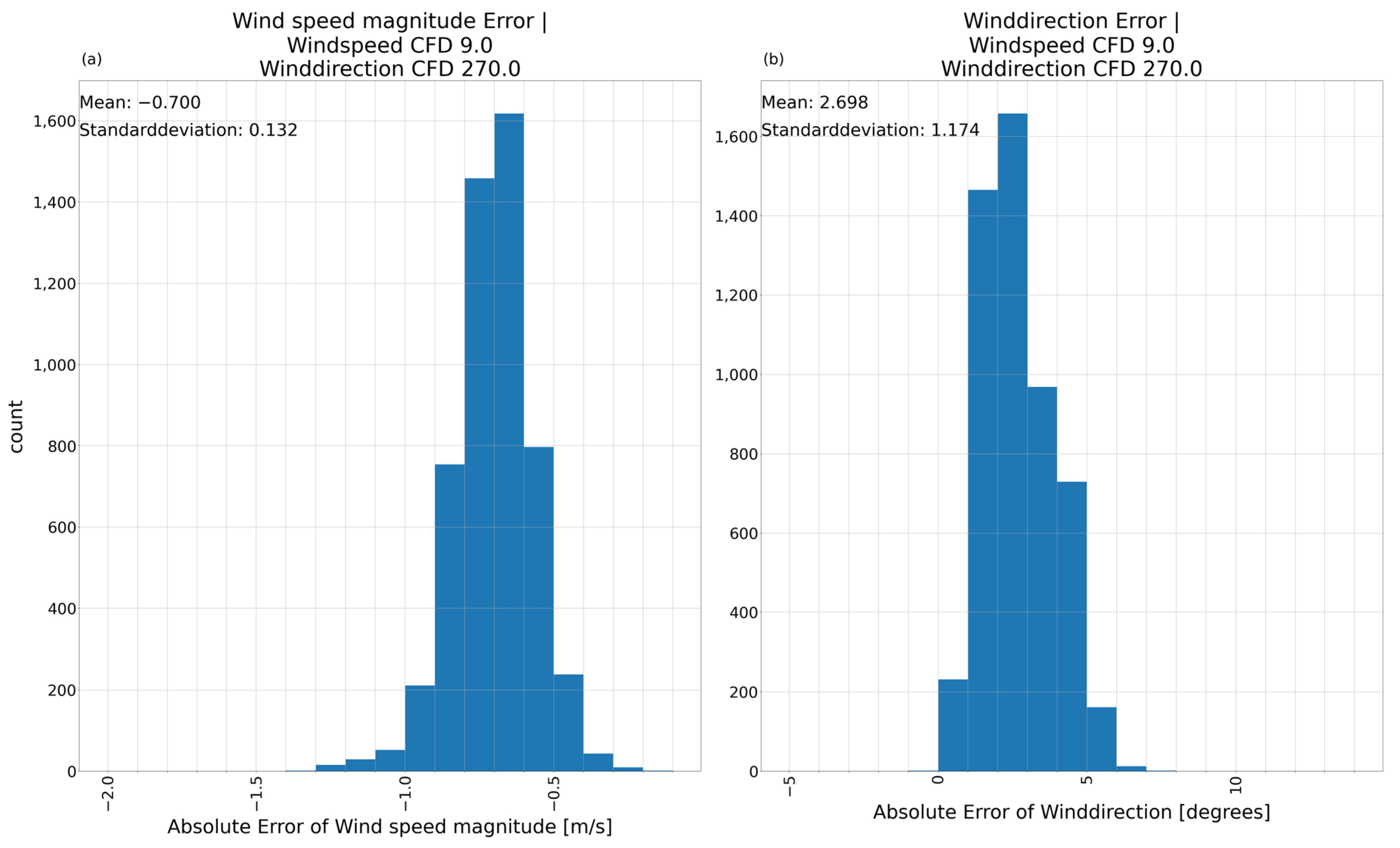
The mean absolute error (VAE2) for reference input 2 is −0.700 for the wind speed (Figure 19a) with a standard deviation of 0.132. The wind direction has a mean absolute error of 2.698 with a standard deviation of 1.174 (Figure 19b). This model also has quite different distributions of errors for different inputs. The difference between the results for different inputs is significantly lower than for the AE-model and for the VAE1-model.

Figure 19. Absolute error histogram between VAE2-model prediction and CFD-simulation for reference input 2 including mean error and standard deviation. (a) Absolute error of the wind speed magnitude; (b) absolute error of the wind direction. Reference input 2.

To evaluate the similarity of two images besides a visual inspection the Structural Similarity Index Measurement (SSIM) is used (Table 6). The CFD-reference is compared to the predictions of the three models. The SSIM for the wind speed does not differ much between the three models. They showed the ability to reproduce areas of the same wind speed close to the CFD-reference albeit mostly with a lower wind speed. The SSIM of the wind direction is highest for the AE-model, matching the CFD-reference closest by structural reproduction and values. Both VAE-models are evenly matched, with only a minor advantage for the VAE2-model.

Table 6. Structural Similarity Index comparing the prediction of each model with the CFD-reference for reference input 2.

Model	SSIM Wind Speed	SSIM Wind Direction
AE	0.99	0.98
VAE1	0.98	0.94
VAE2	0.99	0.95

3.2.3. Evaluation of Model Variations on a Complete Input Dataset

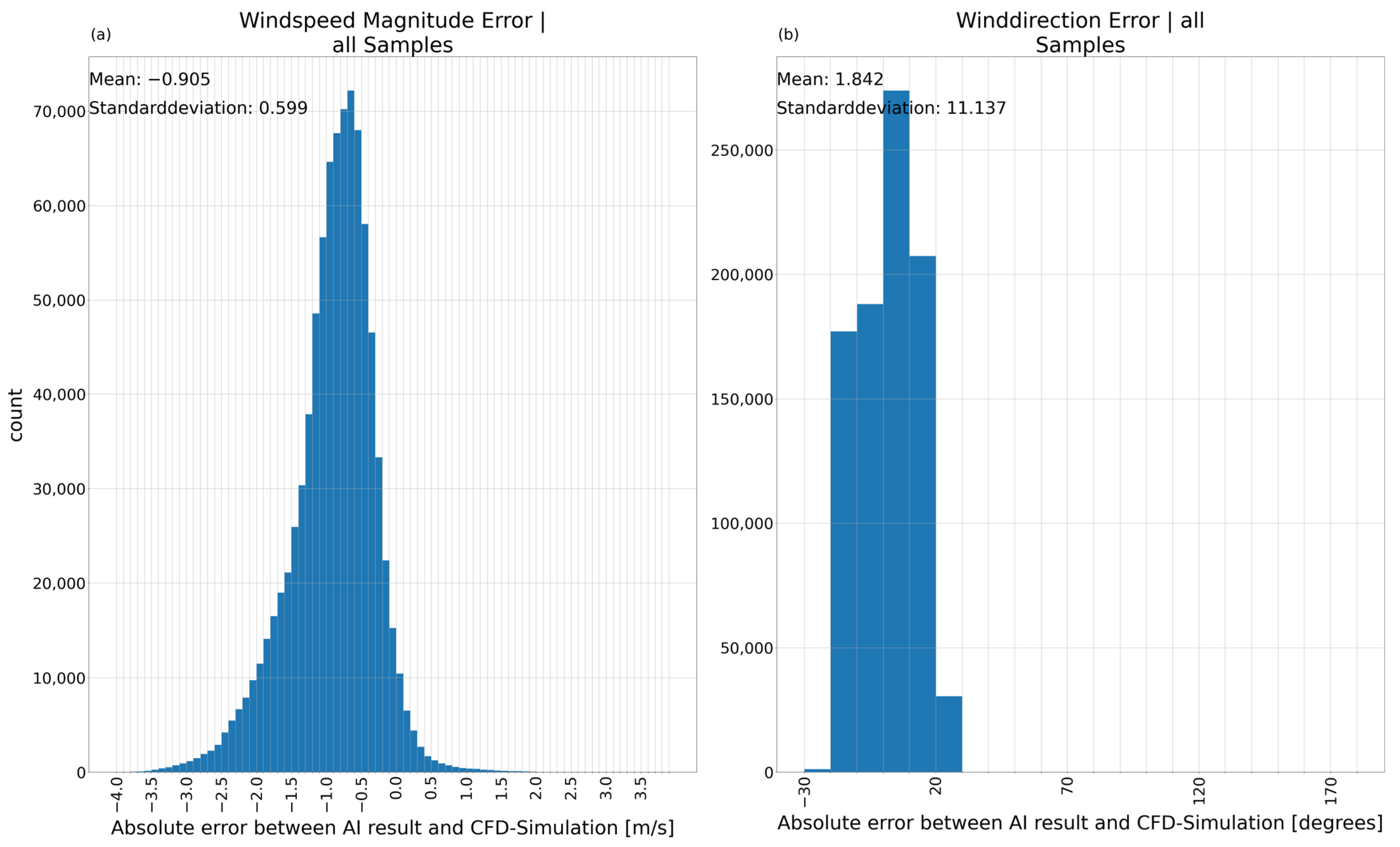
Looking at the error histogram for complete input dataset for the wind speed (Figure 20a) has a maximum at −0.7 m/s. The mean absolute error is −0.905 with a standard deviation of 0.599. Despite the small medium error and small standard deviation, the wind speed errors vary from −4 m/s to +2 m/s, showing a large range which could be attributed to large difference between the predictions on different inputs. Figure 20b shows the distribution of errors for the wind direction. The main peak is between 0 and 10 degrees. The mean absolute error of 1.842 is in the expected range from the first to reference inputs. The standard deviation of 11.137 is quite large and reflects the different qualities of predictions the model produces. Considering Figure 10 and Figure 20 suggests the example of an input wind speed of 8 m/s at 180 degrees is part of a larger set of inputs with similar error distribution.

Figure 20. Absolute error between AE-model prediction and CFD-simulation including mean error and standard deviation for the complete real wind dataset. (a) Absolute error of the wind speed magnitude; (b) absolute error of the wind direction.

Figure 7 shows the result of the AE-model being a good first step with need for further improvements. The histograms in Figure 10 and Figure 20 emphasize necessary improvement of mean absolute error and the standard deviation and a more robust prediction for all inputs.

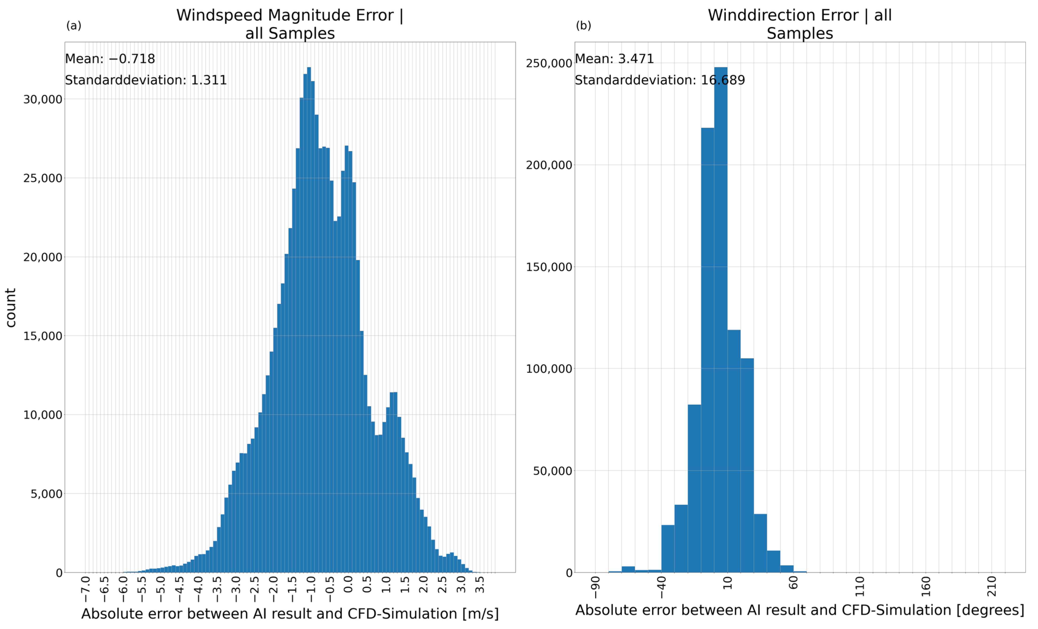
Compared to the results of the AE (Figure 20) the VAE1-model (Figure 21) shows no general improvement in mean absolute error and standard deviation. On the contrary, the standard deviation for both wind speed and wind direction increased. The wind speed show errors between a maximum of −6.5 and +3.5 m/s. The wind direction has large errors of up to −90/+60 degrees albeit a large amount of data being close to the CFD-reference keeping the mean errors relatively small. As stated previously, this is expected to improve for both models with more data.

Figure 21. Absolute error between VAE1-model prediction and CFD-simulation including mean error and standard deviation for the complete real wind dataset. (a) Absolute error of the wind speed magnitude; (b) absolute error of the wind direction.

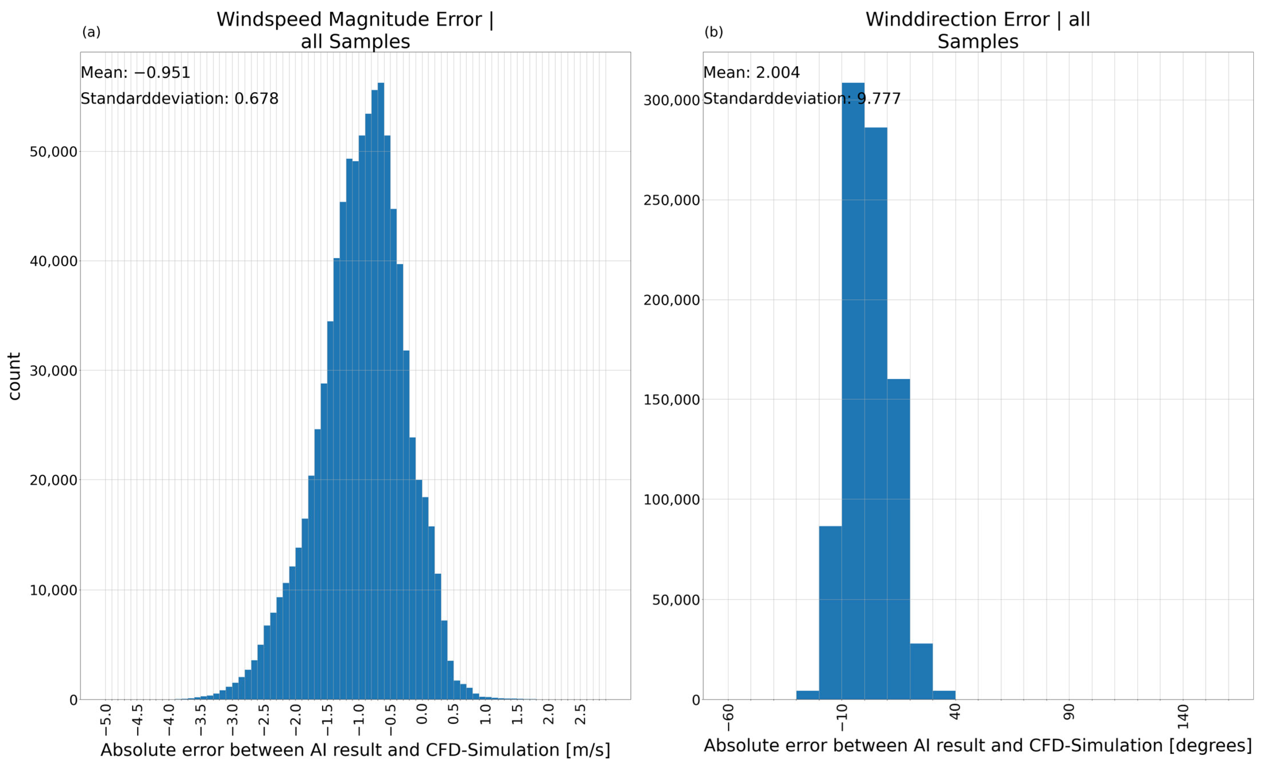
The VAE2-model improves on this rather varied result of the VAE1. The distribution of the errors on all samples in Figure 22 shows a range from −4.5 and +3 m/s. The mean absolute error of the wind speed (Figure 22a) is −0.951 with a corresponding standard deviation of 0.678. Figure 22b shows a mean absolute error of 2.004 and a standard deviation of 9.777 for the error of the wind direction. The VAE2-model managed to improve the mean absolute error and standard deviation of the wind speed to a level comparable to the AE-model while surpassing the AE-model in the standard deviation of the wind direction slightly with a comparable mean absolute error.

Figure 22. Absolute error between VAE2-model prediction and CFD-simulation including mean error and standard deviation for the complete real wind dataset. (a) Absolute error of the wind speed magnitude; (b) absolute error of the wind direction.

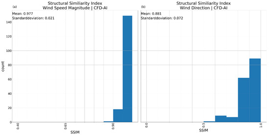
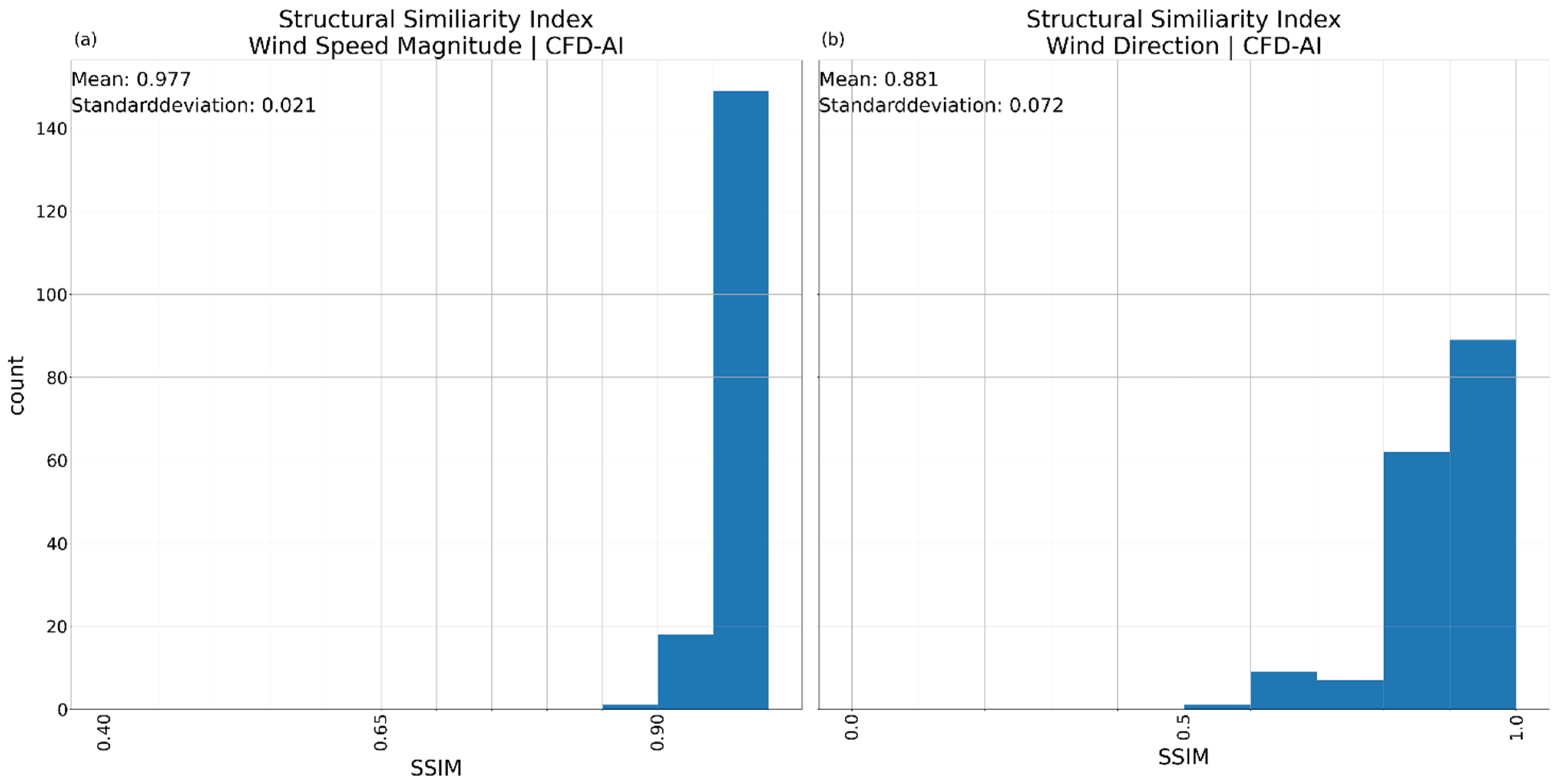
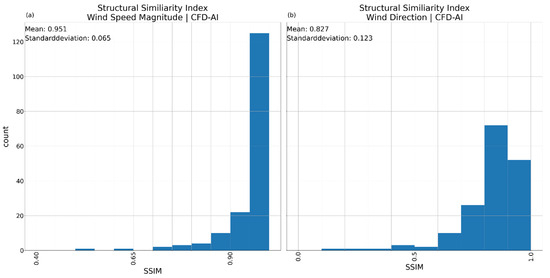
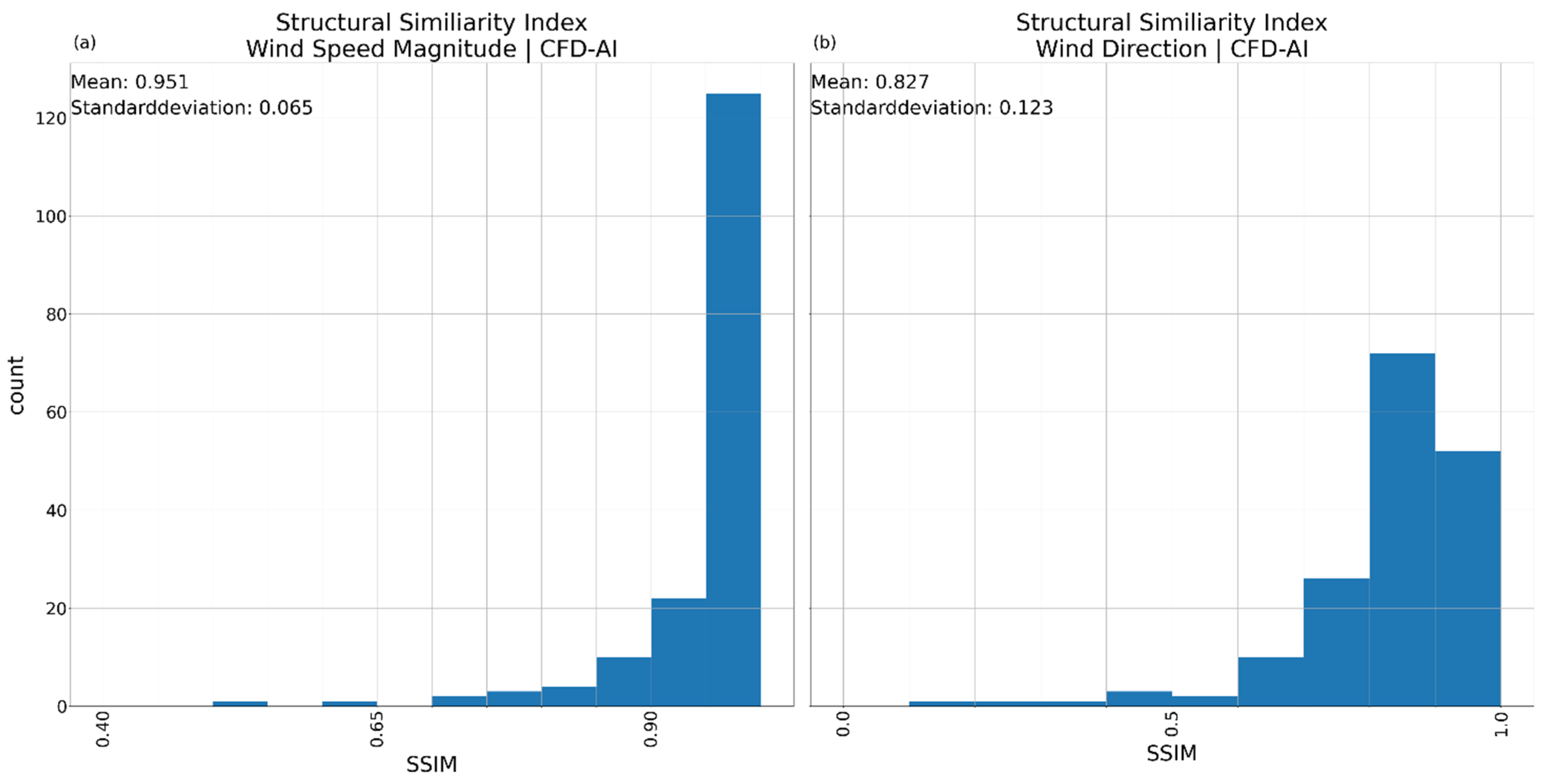
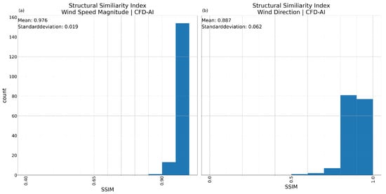
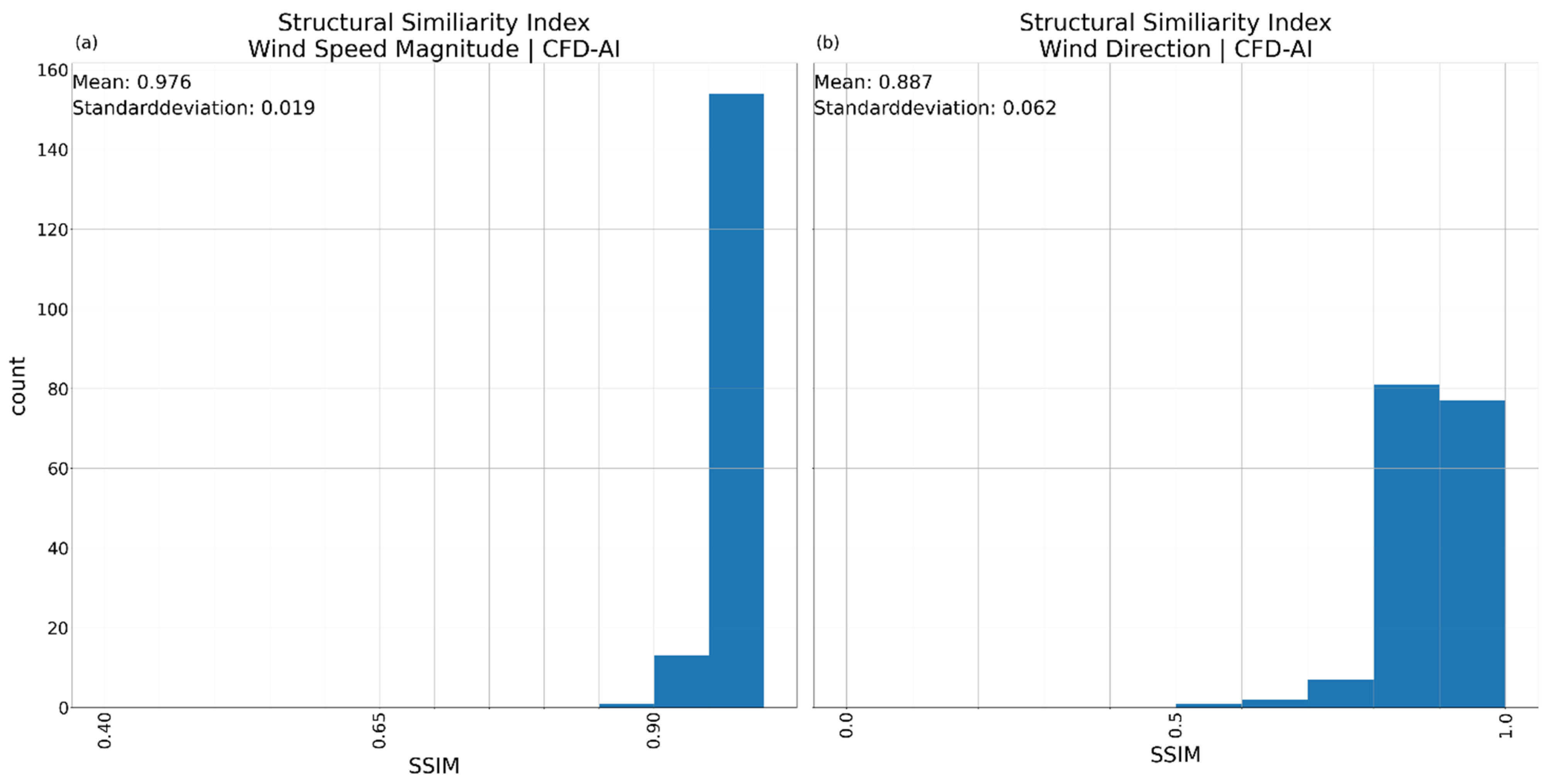
A comparison of the distribution of the SSIM results for the complete input dataset shows a slightly better result for the VAE2-model compared to the AE-model. The VAE1-model performed worse than the two other variants.

The SSIM comparing wind speeds with the CFD-reference shows the AE-model (Figure 23a) delivering a solid performance, the VAE1 model (Figure 24a) exhibits a lower mean SSIM and higher variability and the VAE2-model (Figure 25a) performs on parwith the AE model. The VAE1-model shows SSIM down to 0.5 for some inputs, while the AE- and VAE2-model have only a few inputs with an SSIM between 0.8 and 0.9.

Figure 23. Distribution of all Structural Similarity Index Measurements (SSIMs) for the AE-model comparing the results for the complete real-wind dataset with the appropriate CFD-reference. (a) SSIM for wind speed; (b) SSIM for wind direction.

Figure 24. Distribution of all Structural Similarity Index Measurements (SSIMs) for the VAE1-model comparing the results for the complete real-wind dataset with the appropriate CFD-reference. (a) SSIM for wind speed; (b) SSIM for wind direction.

Figure 25. Distribution of all Structural Similarity Index Measurements (SSIMs) for the VAE2-model comparing the results for the complete real-wind dataset with the appropriate CFD-reference. (a) SSIM for wind speed; (b) SSIM for wind direction.

A similar result can be seen for the SSIM of the wind direction (Figure 23b, Figure 24b and Figure 25b). The AE- and VAE2-model generate no results with an SSIM below 0.5, while the VAE1-model has some outlier results in an SSIM for the wind direction between 0.1 and 0.2, with most results having an SSIM of 0.8 or higher. The VAE1-model, however, seems to have problems reconstructing the areas of same wind direction in some cases.

The better reconstruction shown by the VAE2-model can be attributed to the lower Kullback–Leibler loss factor, increasing the importance of the reconstruction loss, which is the only loss function affecting the AE-model.

4. Discussion

An overview of the performance metrics is detailed in Table 7, which complements the following discussion.

Table 7. Metrics describing the performance of each model variant for reference input 1 (RI1), reference input 2 (RI2) and for the complete input dataset (All) including mean absolute error and standard deviation for the wind speed magnitude, mean absolute error and standard deviation for the wind direction, and the SSIM for wind speed magnitude and wind direction. The SSIM for the complete input dataset is the mean SSIM. The data for the “All” includes bootstrap standard errors employing 10,000 iterations.

	RI1			RI2			All
	AE	VAE1	VAE2	AE	VAE1	VAE2	AE	VAE1	VAE2
Mean absolute error wind speed	1.944	0.534	1.174	0.767	1.384	0.700	0.905 ± 0.035	0.718 ± 0.063	0.951 ± 0.043
Standard deviation wind speed	0.860	0.244	0.247	0.169	0.258	0.132	0.599 ± 0.011	1.311 ± 0.017	0.678 ± 0.008
Mean absolute error wind direction	8.206	2.166	1.419	0.836	5.669	2.698	1.842 ± 0.420	3.471 ± 0.881	2.004 ± 0.437
Standard deviation wind direction	2.621	1.273	0.753	0.535	1.020	1.174	11.137 ± 0.064	16.689 ± 0.126	9.777 ± 0.036
SSIM wind speed	0.92	0.99	0.98	0.99	0.98	0.99	0.977 ± 0.002	0.951 ± 0.005	0.976 ± 0.001
SSIM wind direction	0.70	0.92	0.96	0.98	0.94	0.95	0.881 ± 0.006	0.827 ± 0.009	0.887 ± 0.005

The AE-model shows quite varied results between reference input 1 and reference input 2. The AE-model has the largest mean absolute error of all models for wind speed and wind direction for reference input 1. Especially areas of high wind speed are not reproduced in a recognizable way, predicting wind speeds 2–3 m/s lower than the CFD-reference suggests. The SSIM suggests that the patterns of both wind speed and wind direction were only loosely matched. VAE1 and VAE2 handled this reference input a lot better, VAE1 showing the best result for wind speed error and standard deviation while VAE2 managed to match the wind direction closer to the CFD-reference. VAE1- and VAE2-model both got an excellent SSIM for wind speed of 0.99 and 0.98 respectively, indicating the reproduction of wind fields that match the structure of the CFD-reference quite well albeit with small speed differences. The wind direction of VAE2 shows the best result for reference input 1 with a mean absolute error of just −1.4 degrees and a standard deviation of 0.75, with the VAE1 being a close second place. The SSIM for wind direction shows the VAE2 reconstruction the directions of the wind field matching closely but not perfectly to the CFD-reference. The AE-model had difficulties with the wind directions for this input showing a wind direction error of around 10 degrees for large parts of the evaluated area. As this error is fluctuating a lot, the result of the AE-model shows some differences to the CFD-reference resulting in a low SSIM.

Reference input 2 changes this picture completely, with the AE-model producing a near prefect approximation of the CFD-reference shown by the SSIM of 0.99 and 0.98 for wind speed and wind direction respectively. The mean absolute error for this scenario reinforces this with a small negative mean absolute error and a small standard deviation. The wind direction follows the same pattern with a small negative mean absolute error and a small standard deviation. The VAE1-model, which reproduced the wind speed of reference input 1 best, has the largest mean absolute error for wind speed overestimating wind speed. VAE1 has the largest error in wind direction as well. However, the SSIM shows that the structures seen in the CFD-reference wind speed and wind direction are kept mostly. VAE2 manages to predict the wind speeds equally good to the AE-model but shows a larger error for the wind direction.

Looking at the mean values covering the complete input dataset shows the ability of all three models to predict wind speeds from an input close to a respective CFD-reference. VAE1 shows the smallest mean absolute error here, which is counteracted by the largest standard deviation. The AE- and VAE2-models are slightly worse on the mean absolute error but have a standard deviation about half as large as VAE1 has. The mean SSIM show a minute difference between AE- and VAE2-model, showing that both are equally able to predict wind speeds in a way resembling the CFD-references. VAE1 is the worst in reconstructing wind speed areas. The results of the wind direction show a similar picture showing VAE2 and AE closely matched. Even though the AE-model has the smallest mean absolute error, VAE2 has a smaller standard deviation. The SSIM follows the same trend with VAE2 being best in matching the wind field directions of the CFD-references.

Additionally, we trained models withholding wind speeds 9–11 m/s. The results (see Table 8) show no relevant changes in mean absolute error and standard deviations.

Table 8. Metrics describing the performance of each model variant for reference input 1 (RI1), reference input 2 (RI2) and for the complete input dataset (All) for reduced training data, excluding wind speeds 9–11 m/s.

	RI1			RI2			All
	AE	VAE1	VAE2	AE	VAE1	VAE2	AE	VAE1	VAE2
Mean absolute error wind speed	1.712	1.137	1.238	1.064	1.257	0.692	1.018	0.785	0.6825
Standard deviation wind speed	0.753	0.432	0.24	0.413	0.358	0.149	0.64	1.315	0.625
Mean absolute error wind direction	5.977	4.281	2.314	1.951	6.931	0.812	0.747	1.258	0.825
Standard deviation wind direction	2.334	1.687	1.156	1.335	1.412	0.856	10.482	17.297	9.769
SSIM wind speed	0.93	0.98	0.98	0.98	0.97	0.99	0.972	0.949	0.984
SSIM wind direction	0.76	0.87	0.94	0.89	0.89	0.97	0.864	0.820	0.892

In total, VAE2 is the best model of the three tested models, showing the best stability for predicting the wind speed and direction over terrain and forested area for input data not including terrain and/or forest effects on wind speeds and directions.

A larger training dataset incorporating more wind directions can further improve the performance of all models; it would provide more reference simulations to compare the results to. As the training for those models happened on limited data, it is expected that each model can have shortfalls for some input scenarios like the AE possibly shows on reference input 1. A larger training dataset would improve prediction performance for the models.

5. Limitations

The models were trained for a single topography to validate the general approach. Generalization across different topography is not possible based upon this training. Using the model on different topography currently ignores the topography and emulates wind fields with the according wind speed and direction learned on the trained topography. Transfer beyond the current site requires training on multiple locations, which is the scope of future work.

6. Conclusions

In this study we used a set of high resolution CFD-simulations of wind fields to train three variations of CNNs to downscale wind data at a reference site and improve the adherence to terrain and forest influencing wind speed and wind direction. The available wind data from Nefino is reanalysis data already downscaled by their interpolation method and does not capture influences of terrain and forest well.

The CNN variations tested on the reanalysis data from Nefino are an autoencoder and two variations of a variational autoencoder with matching structure. For the comparison of the models, two reference inputs were used as well as an overview over all available reanalysis data. For each input, the closest matching available CFD-simulation was used as ground truth, and mean absolute error, standard deviation and structural similarity index measurement are compared.

The autoencoder (AE) demonstrates low mean absolute errors and standard deviations when compared to a CFD-reference simulation, but it underestimates peak wind speeds. This model also shows difficulties with the prediction of wind speed and especially wind direction of reference input 1 while doing a near perfect representation of the CFD-reference for reference input 2. In general, the AE did a good job capturing wind speeds but shows large errors for the wind direction. Variational Autoencoder 1 (VAE1) shows fundamentally improved visual results and better reconstruction of wind pattern shown also by the high SSIM for both reference inputs. On the other hand, results of VAE1 suffer from a high variability in wind direction with large errors in some cases. The Variational Autoencoder 2 model using factor_kl = −0.05 performs well at the reference inputs, surpassing AE at reference input 1 and having a slightly larger error of wind direction for reference input 2. For the complete set of input wind fields, VAE2 matches the accuracy of the AE for wind speed reconstruction and improves on the prediction of the wind direction. VAE2 is a good candidate for further improvements to improve on consistent predictions for varying wind speeds and directions.

As there was no optimization of the models, there is much room of improvement in that regard to increase accuracy of the model predictions. Furthermore, the training data covered a lot of different wind speeds, but only 12 wind direction were included in the data. A larger dataset containing finer resolved wind directions is expected to improve the results of the VAE2-model and lead to smaller errors in the predictions. The models were trained on a single topography. For the models to be useable on more than one topography, training needs to include several different reference locations, possibly leading to a generalization by the VAE-model for unseen locations.

This would lead to an AI-model giving fast access to high-resolution terrain dependant wind fields based on coarse but widely available predictions by meteorological services. An improved model could also be used to process large amounts of reanalysis data, improving the resolution of wind forecasts over forests and complex terrain. Those fast-to-compute high-resolution wind fields can be highly beneficial, for example in firefighting, wind power modelling or other applications where wind speeds over local terrain are important.

References

- Raupach, M.R. Vegetation-atmosphere interaction and surface conductance at leaf, canopy and regional scales. Agric. For. Meteorol. 1995, 73, 151–179. [Google Scholar] [CrossRef] [Scilit]
- Skamarock, W.C.; Klemp, J.B.; Dudhia, J.; Gill, D.O.; Liu, Z.; Berner, J.; Wang, W.; Power, J.G.; Duda, M.G.; Barker, D.M.; et al. A Description of the Advanced Research WRF Model Version 4; National Center for Atmospheric Research: Boulder, CO, USA, 2021. [Google Scholar]
- Floors, R.; Enevoldsen, P.; Davis, N.; Arnqvist, J.; Dellwik, E. From lidar scans to roughness maps for wind resource modelling in forested areas. Wind Energy Sci. 2018, 3, 353–370. [Google Scholar] [CrossRef] [Scilit]
- Larsson, R.; Rudberg, M. Impact of Weather Condidtions on In Situ Concrete Wall Operations Using a Simulation-Based Approach. J. Constr. Eng. Manag. 2019, 145, 05019009. [Google Scholar] [CrossRef] [Scilit]
- Mohamend, E.; Jafari, P.; Chehouri, A.; AbouRizk, S. Simulation-Based Approach for Lookahead Scheduling of Onshore Wind Projects Subject to Weather Risk. Sustainability 2021, 13, 10060. [Google Scholar] [CrossRef] [Scilit]
- Alessi, M.J.; DeGaetano, A.T. A comparison of statistical and dynamical downscaling methods for short-term weather forecasts in the US Northeast. Meteorol. Appl. 2021, 28, e1976. [Google Scholar] [CrossRef] [Scilit]
- Wilby, R.L.; Wigley, T.M.L. Downscaling general circulation model output: A review of methods and limitations. Prog. Phys. Geogr. Earth Environ. 1997, 21, 530–548. [Google Scholar] [CrossRef] [Scilit]
- Labeurthre, D.; Reffet, A.; Schrapffer, A. An Overview of Statistical Downscaling Methods: Techniques, Applications, and Advances. SSRN 2025. Available online: https://www.researchgate.net/publication/388472320_An_Overview_of_Statistical_Downscaling_Methods_Techniques_Applications_and_Advances (accessed on 9 December 2025).
- Olivares-Espinosa, H.; Arnqvist, J. Modelling of wind flows over realistic forests with LES. Wind Energy Sci. Discuss. 2025, 2025, 1–48. [Google Scholar]
- Olivares-Espinosa, H.; Arnqvist, J. Modelling of wind turbine wakes over forests along diurnal cycle. J. Phys. Conf. Ser. 2023, 2505, 12043. [Google Scholar] [CrossRef] [Scilit]
- Letzgus, P.; Guma, G.; Lutz, T. Computational fluid dynamics studies on wind turbine interactions with the turbulent local flow field influenced by complex topography and thermal stratification. Wind Energy Sci. 2022, 7, 1551–1573. [Google Scholar] [CrossRef] [Scilit]
- Ivanell, S.; Arnqvist, J.; Avila, M.; Cavar, D.; Chavez-Arroyo, R.A.; Olivares-Espinosa, H.; Peralta, C.; Adib, J.; Witha, B. Micro-scale model comparison (benchmark) at the moderately complex forested site Ryningsnäs. Wind Energy Sci. 2018, 3, 929–946. [Google Scholar] [CrossRef] [Scilit]
- Ericson, W.; Achermann, F.; Lawrance, N.; Villinger, J.; Andersson, O.; Siegwart, R. Evaluating machine-learning models for wind-speed downscaling from ECMWF-IFS data. Q. J. R. Meteorol. Soc. 2025, 151, e5063. [Google Scholar] [CrossRef] [Scilit]
- Miralles, O.; Steinfield, D.; Martius, O.; Davison, A.C. Downscaling of Historical Wind Fields over Switzerland using Generative Adversarial Networks. Artif. Intell. Earth Syst. 2022, 1, e220018. [Google Scholar] [CrossRef] [Scilit]
- Dujardin, J.; Lehning, M. Wind-Topo: Downscaling near-surface wind fields to high-resolution topography in highly complex terrain with deep learning. Q. J. R. Meteorol. Soc. 2022, 148, 1368–1388. [Google Scholar] [CrossRef] [Scilit]
- Zhang, X.; Zhang, T.; Ke, S.; He, H.; Zhang, R.; Miao, Y.; Liang, T. Physics-Informed Deep Learning for 3D Wind Field Retrieval of Open-Ocean Typhoons. Remote Sens. 2025, 17, 3825. [Google Scholar] [CrossRef] [Scilit]
- Milla-Val, J.; Montañés, C.; Fueyo, N. An image-to-image adversarial network to generate high resolution wind data over complex terrains from weather predictions. Eng. Appl. Artif. Intell. 2025, 139, 109533. [Google Scholar] [CrossRef] [Scilit]
- Lin, C.; Tie, R.; Yi, S.; Zhong, X.; Li, H. Terrain-aware Deep Learning for Wind Energy Applications: From Kilometer-scale Forecasts to Fine Wind Fields. arXiv 2025, arXiv:2505.12732. [Google Scholar]
- IG Windkraft Austrian Wind Energy Association. IG Windkraft—Windkraft am Berg. 25 July 2022. Available online: https://web.archive.org/web/20230326223757/https://www.igwindkraft.at/?xmlval_ID_KEY%5b0%5d=1332 (accessed on 16 January 2025).
- Staffell, I.; Green, R. How does wind farm performace decline with age? Renew. Energy 2014, 66, 775–786. [Google Scholar] [CrossRef] [Scilit]
- Staffell, I.; Pfenniger, S. Using bias-corrected reanalysis to simulate current and future wind power output. Energy 2016, 114, 1224–1239. [Google Scholar] [CrossRef] [Scilit]
- Gad, A.F. Image Compression Using Autoencoders in Keras|DigitalOcean. 26 September 2024. Available online: https://www.digitalocean.com/community/tutorials/autoencoder-image-compression-keras (accessed on 25 November 2024).
- Gad, A.F. How to Build a Variational Autoencoder in Keras|Paperspace Blog. 2020. Available online: https://blog.paperspace.com/how-to-build-variational-autoencoder-keras/ (accessed on 25 November 2024).
- Chollet, F. Keras. 2015. Available online: https://keras.io (accessed on 10 December 2025).
- Abadi, M.; Agarwal, A. TensorFlow: Large-Scale Machine Learning on Heterogenous Systems. 2015. Available online: https://www.tensorflow.org (accessed on 16 February 2026).
- Kromydas, B. Convolutional Neural Network (CNN): A Complete Guide. 18 January 2023. Available online: https://learnopencv.com/understanding-convolutional-neural-networks-cnn/ (accessed on 10 December 2024).
- Monshizadeh, M.; Khatri, V.; Gamdou, M.; Kantola, R.; Yan, Z. Improving Data Generalization with Variational Autoencoders for Network Traffic Anomaly Detection. IEEE Access 2021, 9, 56893–56907. [Google Scholar] [CrossRef] [Scilit]
- Higgins, I.; Matthey, L.; Pal, A.; Burgess, C.; Glorot, X.; Botvinick, M.; Mohamed, S.; Lerchner, A. beta-VAE: Learning Basic Visual Concepts with a Constrained Variational Framework. ICLR 2017 Poster. 2017. Available online: https://openreview.net/forum?id=Sy2fzU9gl (accessed on 18 January 2026).
- Pykes, K. Variational Autoencoders: How They Work and Why They Matter. 13 August 2024. Available online: https://www.datacamp.com/tutorial/variational-autoencoders (accessed on 4 February 2025).
- Wang, Z.; Bovik, A.C.; Sheik, H.R.; Simoncelli, E.P. Image quality assessment: From error visibility to structural similarity. IEEE Trans. Image Process. 2004, 13, 600–612. [Google Scholar] [CrossRef] [Scilit] [PubMed]
Disclaimer/Publisher’s Note: The statements, opinions and data contained in all publications are solely those of the individual author(s) and contributor(s) and not of MDPI and/or the editor(s). MDPI and/or the editor(s) disclaim responsibility for any injury to people or property resulting from any ideas, methods, instructions or products referred to in the content. |
© 2026 by the authors. Licensee MDPI, Basel, Switzerland. This article is an open access article distributed under the terms and conditions of the Creative Commons Attribution (CC BY) license.