


Abstract
Vertical-axis wind turbines (VAWTs) could be a good alternative to horizontal axis turbines for offshore applications. However, the variability of the aerodynamic forces with the blade azimuthal position subjects the blade to fatigue stresses and generates typical power periodicity. Extreme wind conditions, such as gusts, could aggravate the aerodynamic load peaks, compromising the system durability. We analyze the transient aerodynamic loads generated under gusty winds for a 5 MW offshore troposkein-shaped VAWT. The behavior of the turbine at its equatorial plane is simulated by 2D-CFD assuming gusts characterized by different periods and amplitudes. Since the turbine is stall-regulated, a range of wind velocities going from the maximum efficiency velocity to the nominal power velocity are considered. The instantaneous overloads of power, blade radial force, and total force on the shaft are analyzed. An increase in the peak values up to 119% (power) and 51% (force on the shaft) are predicted relative to the most severe steady condition, depending on gust characteristics and the blade position when the gust crest occurs. These results refer to the equatorial plane, rather than the entire turbine. It is demonstrated how the passive stall load regulation method protects the turbine from excessive overloads.
1. Introduction
A growing interest in vertical-axis wind turbines (VAWTs) is emerging in large-scale offshore applications. The advantages, compared to traditional horizontal-axis turbines, are well known: lower installation costs (construction simplicity, lower material costs), no need for a yaw system (the turbine works regardless of the wind direction), low gravity center (no nacelle, very short tower, electrical equipment located at the base of the turbine), and therefore great stability when using a floating platform suitable for deep water. The main disadvantage that penalizes VAWTs is the variation, during each revolution, of the fluid dynamic interaction between the incoming flow and the blade; in fact, the inflow angle and the magnitude of the relative velocity to the blade depend on the instantaneous angular position of the blade. Consequently, the torque, the power output, and all the loads transmitted to the components of the system fluctuate periodically. It is therefore crucial to investigate, through experiments or numerical methods, the effects that extreme winds, such as sudden gusts, could have on the blades, the connecting arms, and the tower, which are already subject to significant fatigue stresses due to the intrinsic operating modes of this type of turbine.
The literature reports a few studies concerning VAWTs, some of which are about the effects of unsteady periodically fluctuating winds on turbine performance [1,2,3,4,5,6,7,8]. In particular, Yu et al. [4] conducted a systematic study on the gust response in terms of torque, power output, and aerodynamic behaviors of a VAWT that is expected to operate in an urban environment, also including asymmetric oblique gusts; Wu, Bangga, and Cao [5] analyzed the performance of a three-bladed VAWT under the effect of sinusoidal gusts with various directions (i.e., including lateral gusts), velocity amplitudes, and frequencies; Danao et al. [6] and Bhargav el al. [7] investigated the amplitude and frequency effects of sinusoidal wind speed fluctuations on the power coefficient, , of small-scale VAWT; and Wekesa et al. [8] focused on increasing the energy capture achievable for small turbines from short-period fluctuating winds, typical of realistic environments.
The effects of single “Extreme Operating Gust” (EOG) events, characterized by sudden increases and decreases in wind speed, have been studied for small turbines to reproduce realistic urban/suburban environments [9,10,11], also considering high turbulence levels [10]. Rakib, Evans, and Clausen [11] made a comparison between the effects of experimental gusts and gusts modeled with standardized approaches.
However, the cases mentioned so far focus only on the power capture and on power fluctuation peaks.
Just few studies can be found on large scale VAWTs [12,13]. Padron et al. [12] developed a multi-fidelity uncertainty quantification approach in which the extreme gust is parameterized by random variables to predict the effects of chaotic realistic gusts on transient power and streamwise force, applying it to a 5 MW case study. The “multi-fidelity” approach refers to a combination of a few high-fidelity 2D CFD simulations with many low-fidelity runs (BEM, vortex lattice). However, since the focus is on the mathematical aspects, the fluid dynamic mechanisms occurring during the gust are almost neglected; the main result they found is that the ability of the high-fidelity solver to predict the gust effects on the maximum forces is crucial as the low-fidelity solver underestimates theme.
In their work Kjellin, Eriksson, and Bernhoff [13] proved that one way to efficiently control the power output even in gusty conditions is to keep the rotation speed constant above the nominal wind speed, since a sudden increase in wind speed causes the turbine to stall, decreasing the impact on the power output.
Nevertheless, to the authors’ knowledge, no systematic studies have considered a wide range of characteristics of extreme winds acting on large-scale VAWTs, nor have any studies considered the instantaneous overloads of both the tangential force (generating power) and the radial forces. The most recent literature shows many examples of VAWTs operating in gusty conditions [14,15,16], but these studies mostly focus on small turbines with a rotor diameter of around 1 m (or a maximum of 1.7 m [15]). The gust events considered are all characterized by a period much longer than that of the turbine. An interesting study is that of Moore et al. [17]: in this case, a troposkein-shaped turbine is studied using a 3D free vortex model. The study considers a gust event with a period comparable to that of the turbine.
The present study would like to contribute to fill this gap. It should be clarified that the purpose of this manuscript is not to indicate a methodology for predicting the maximum loads acting on a given turbine, since full CFD, i.e., “blade resolved”, requires excessive computational resources in both 3D and 2D; other numerical approaches characterized by less accuracy and much greater computation speed would be better suited to this purpose. However, these latter approaches, which are hybrid CFD–Blade-Element Momentum and are called “low orders CFD” (such as the Actuator Cylinder [18], and the Actuator Line models) need to be tuned on a case-by-case basis as they make use of semi-empirical sub-models. Through our research, we aimed to investigate the physical mechanisms that amplify instantaneous aerodynamic overloads. At the same time, we sought to provide a large set of accurate data that could be used by “low orders” model developers for comparison or validation purposes.
2. Methodology
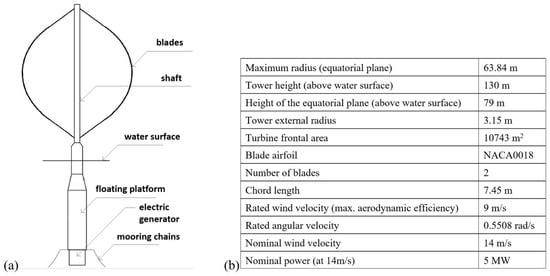
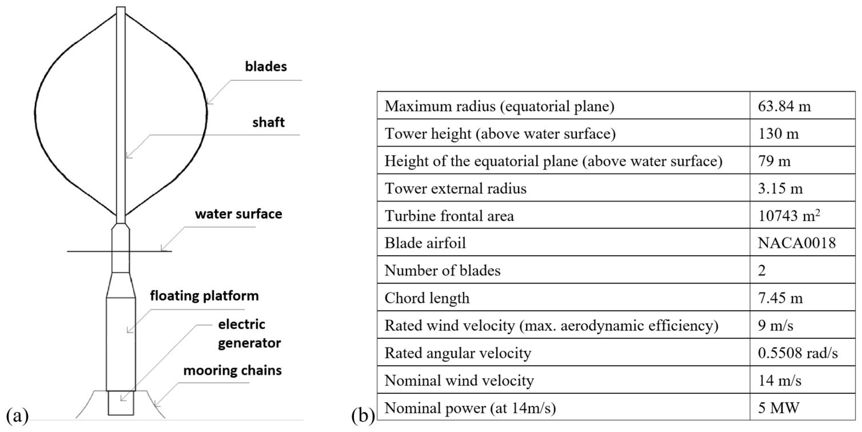
This investigation focuses on a well-known offshore VAWT, named DeepWind (a project funded by the EU). The turbine has a troposkein shape, with a maximum radius, R, of 63.8 m; it has 2 blades with a NACA0018 airfoil profile. Figure 1 shows the main components of the system (including the floating platform) and the geometrical and operational characteristics [19]. A nominal power of 5 MW is expected for a wind speed of 14 m/s. In this condition the turbine should experience stall; in fact, the load is stall-controlled. This means that beyond a given “rated wind speed” (that is 9 m/s) the rotation speed is kept constant in order to induce stall, thereby gradually and significantly reducing the aerodynamic performance. Meanwhile, the wind kinetic power continues to grow with cubic trend.
Figure 1.
(a) Main components of the DeepWind turbine; (b) the geometry and operating conditions of the DeepWind turbine.
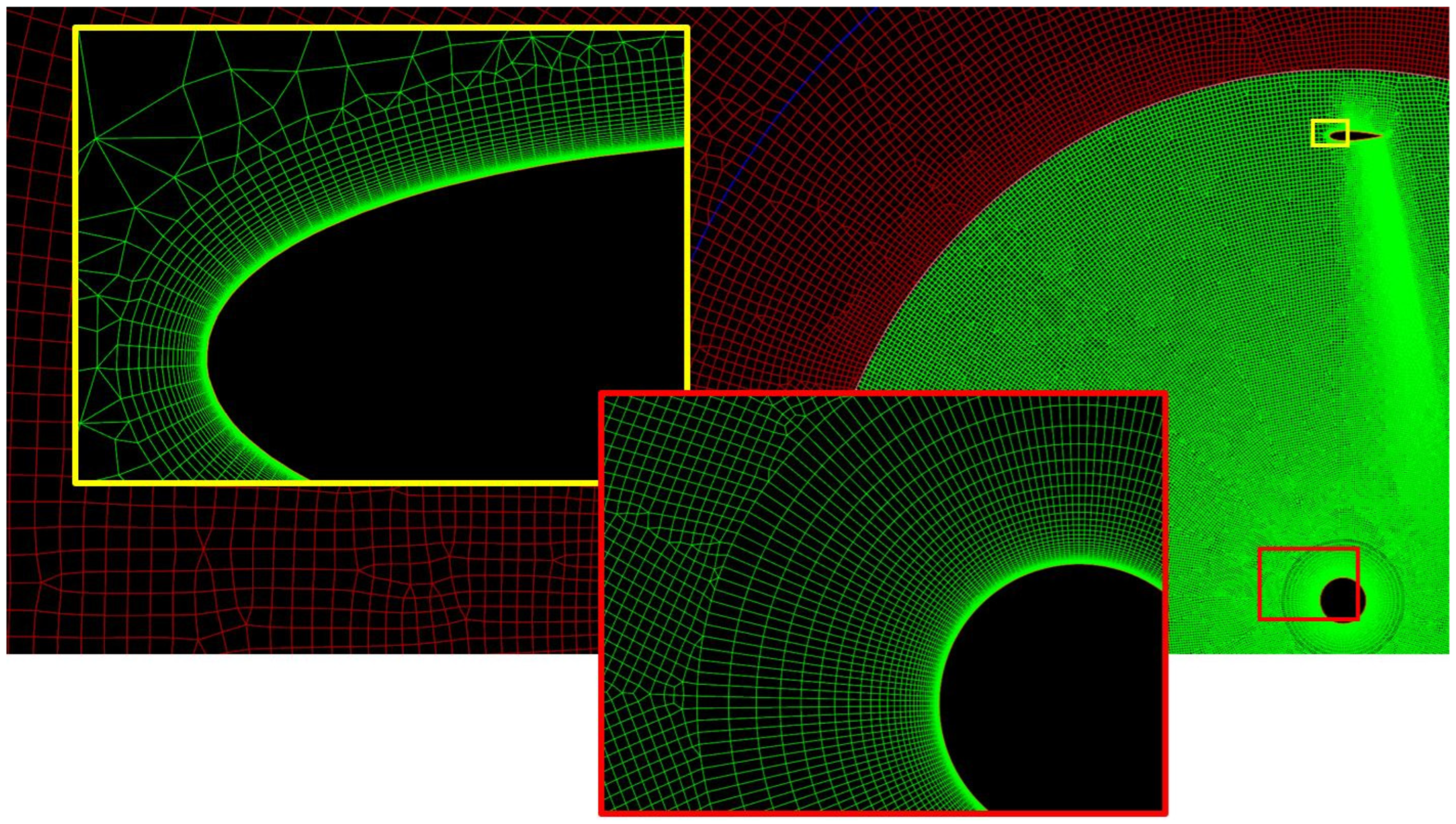
Our study is based on 2D-CFD simulations performed on the equatorial section of the turbine using Ansys-Fluent v19.2 software. The calculation domain is rectangular; indicating with D the turbine diameter, its dimensions are 20∗D in the crosswise direction and 7∗D and 15∗D in the streamwise direction, upstream and downstream respectively. Two grid levels are used to simulate the blade rotation via the sliding mesh method: a fixed sub-grid with the outer dimensions of the flow domain (~5 ∗ 104 cells) and a rotating sub-grid including blades and tower (~1.3 ∗ 105 cells). A boundary condition (BC) “interface” is set at the joint of the two grids. The other BCs are “wall” for the blades and tower, “velocity inlet” for the inlet, “pressure outlet” for the exit, and “symmetry” for the domain sides. The grid is unstructured, made of quad-dominant elements; 400 nodes are placed on each blade contour. Around the walls (blades and tower), ~50 layers of regular quadrilateral cells are employed, as depicted in Figure 2. The height of the first layer of cells is just 5 ∗ 10−6c in order to keep y+ abundantly <1, and c is the chord of the blade.
Figure 2.
In maroon, a small piece of the fixed domain; in green, a partial view of the rotating domain; inside the boxes, grid refinements around the blade (yellow frame) and around the turbine tower (red frame).
To model the turbulence, the k-ω SST (Shear Stress Transport) by Menter [20,21] is adopted; this model is widely used to simulate VAWTs since it is considered well appropriate in case of flow affected by strong adverse pressure and separation, as happens when the turbine works under stall conditions.
The algorithm for the velocity–pressure coupling is SIMPLEC. For the spatial discretization scheme, Least Squares Cell-Based (LSCB) is set for the gradient. Pressure interpolation, turbulent kinetic energy, and specific dissipation rate formulations are based on second order schemes. Temporal discretization is also based on a second order implicit method. The convergence criteria for each time-step is 1 ∗ 10−4 for the continuity, velocity, turbulence kinetic energy, and specific dissipation rate residuals. To obtain a satisfactory numerical convergence in sliding meshes, the time-step should not exceed the time required to advance the mobile interface by a distance corresponding to one cell. Therefore, a value of 0.5° of blade revolution was assumed in the present study, also considering that a value of 0.5° had provided results very close to those obtained with a time-step of 0.25° in a previous study [22]. A detailed sensitivity analysis to the resolution of the computational grid and a validation work of the overall numerical model against experimental data from the literature are reported in Appendix A in order not to distract attention from the aims of this study.
Five wind velocities, , are considered: 9 m/s (the rated wind), 14 m/s (the nominal wind), and three intermediate values; the turbine speed, , is maintained fixed at 0.55 rad/s, and consequently the turbine period is 11.4 s.
The most important parameter characterizing the turbine performance is the Coefficient of Power, , which represents the aerodynamic efficiency. It is defined as the power output, P, divided by the kinetic power available in the wind:
where is the density and A is the turbine frontal area. In 2D CFD the forces, moments and powers, are calculated for 1 m of blade extrusion in the third dimension, therefore in this paper (and not the total area of the turbine). For wind turbines, regardless of whether they are vertical or horizontal axis, the fundamental operating parameter is the Tip Speed Ratio, TSR, defined as the blade tangential speed divided by the wind speed:
It is well known that there is only one value of TSR that maximizes , since at lower TSR the aerodynamic efficiency decreases due to stall, whereas at higher TSR the efficiency decreases due to excessive viscous frictional resistance on the blade surfaces [23].
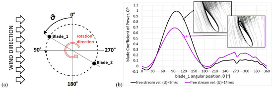
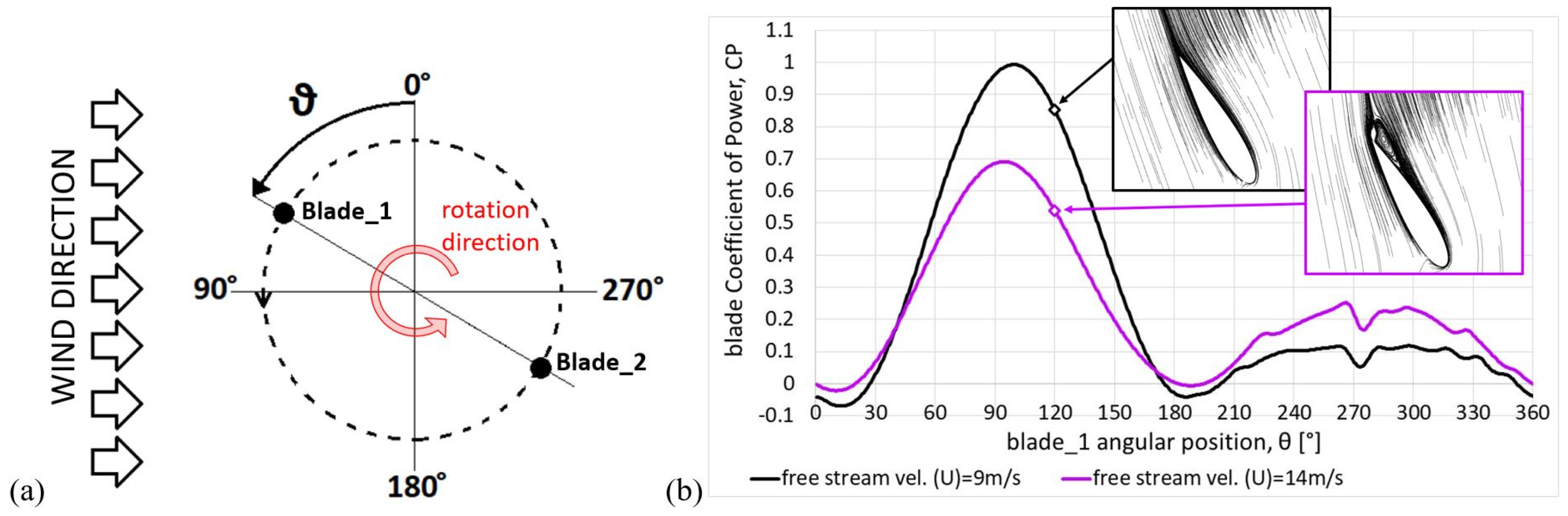
Figure 3 supports considerations that will be useful to understand the results in Section 3. Here θ defines the azimuthal (or angular) position of blade_1 (blade_2 follows by 180°); the blade path between 0° and 180° is usually called “upwind”, while the path between 180° and 360° is called “downwind”. Figure 3b shows the instantaneous for the single blade, predicted during one revolution for = 9 m/s (the designers of the DeepWind turbine expected that at this wind speed the TSR should be the one that maximizes ) and = 14 m/s.
Figure 3.
(a) Definition for the blade angular position; (b) blade during the revolution for wind velocities 9 and 14 m/s; flow details at θ = 120°.
There are two reasons why the torque generated by the blade varies during the revolution. The first is that as θ varies the blade experiences different apparent speeds (vector sum of wind and blade speeds) and attack angles (angle between apparent wind and chord). The second is that during downwind the blade works in the wake, so it can only exploit a reduced wind kinetic power. As can be seen, the maximum occurs ~10° ÷ 15° after the upwind midpoint; at this position the blade experiences the highest attack angle (details are given in Appendix B) and therefore the maximum lift and torque. However, the maximum is much higher at 9 m/s than at 14 m/s, since at 9 m/s the turbine speed is adequate to keep the flow attached, whereas at 14 m/s the attack angle is too large (the turbine is moving too slowly relative to the wind), leading to flow separation (compare the streamlines in the boxes, achieved at θ = 120°) and then to a sudden drag increase.
For each wind speed a preliminary simulation of 25 revs is done to obtain a steady flow field and steady turbine performance. Then, during the 26th revolution, the gust begins. For each gust condition, 20 runs were performed, differing in the relative phase between the blade position and the start of the gust (the first run is for a gust that begins when the blade’s angular position, θ, is 0°). This means increasing the phase difference by 9° each time (for the twentieth run, the gust begins when θ is 171°); obviously, since there are two blades, thanks to the periodicity, it is not necessary to go beyond 171° since the run with the gust beginning when the blade is at 180° would provide identical results to the first run in the series.
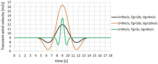
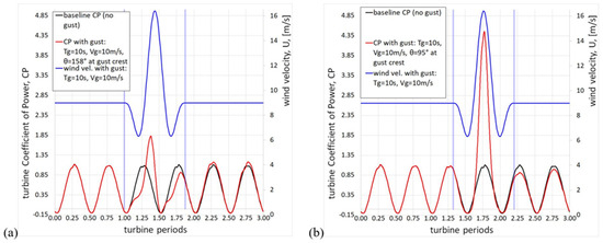
The International Electrotechnical Commission (IEC), a non-governmental organization that establishes safety requirements for wind turbines, has characterized a wind with EOG by means of the following equation where is the transient free stream velocity, is the instant in which the gust begins, is the gust period (or duration) in s, and is the gust amplitude in m/s [24]:
As shown in Figure 4, a gust obtained from Equation (3) is described by a velocity drop followed by a sudden rise to a crest, followed by another drop mirroring the first. We chose 6 gust types (described by Equation (3)), as a combination of two periods (10 s, which corresponds to a statistically very probable value for the seas of Northern Europe; and 3 s) and three amplitudes (4, 6 and 10 m/s).
Figure 4.
Examples of three wind profiles with Extreme Operating Gusts (EOGs) of different periods and amplitudes (from Equation (3)).
3. Results
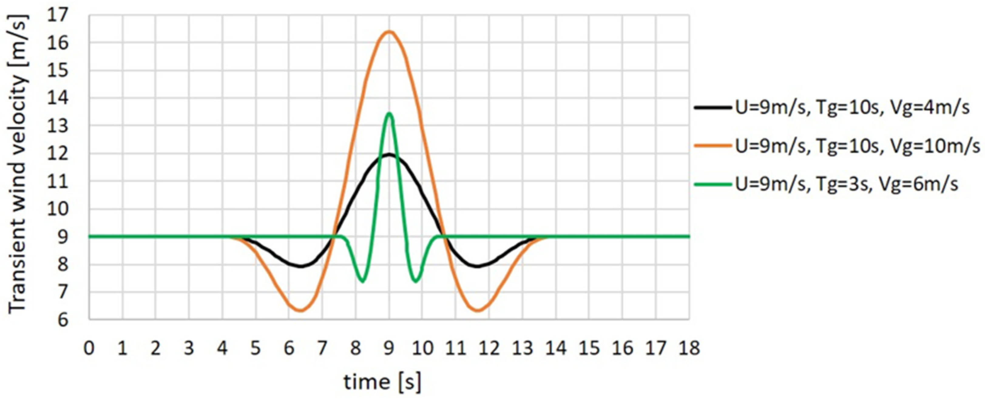
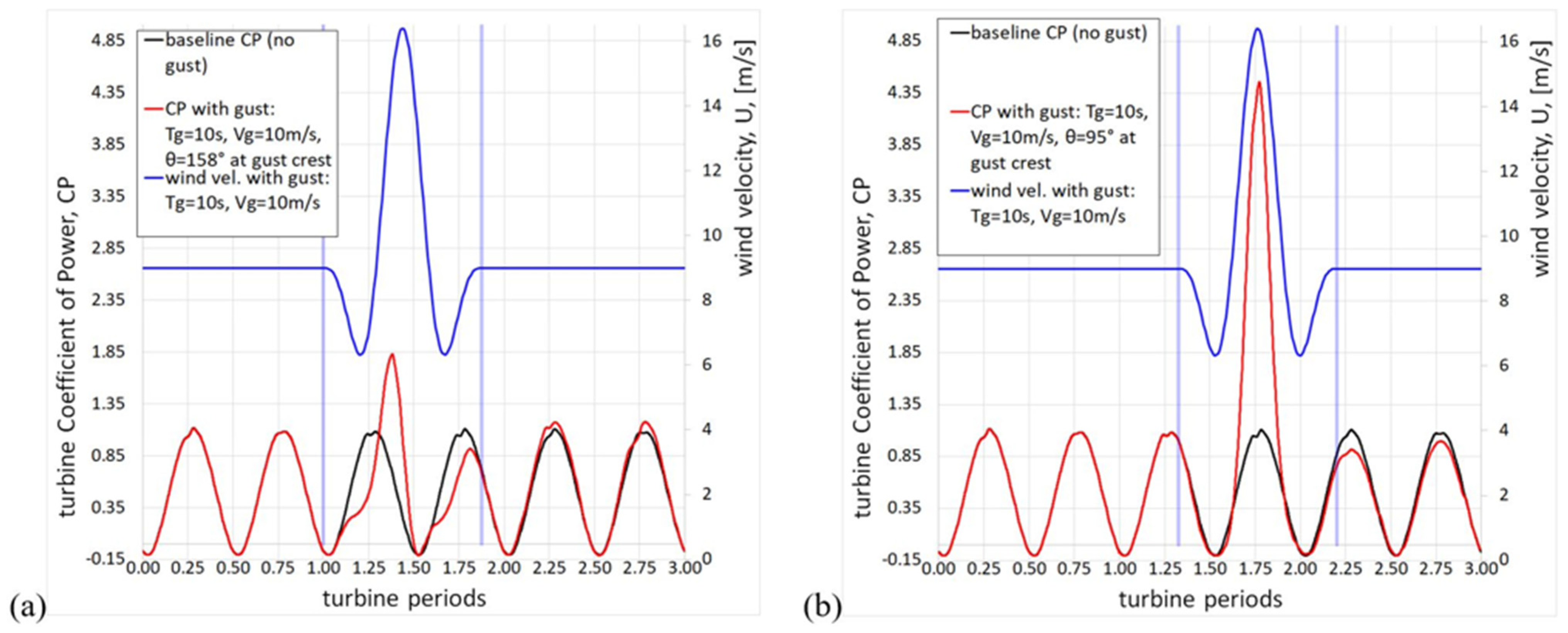
Figure 5a depicts the effects of a gust with = 10 s and = 10 m/s on the turbine (sum of the of the two blades) for a steady wind speed of 9 m/s, in comparison to the case without gust. It must be specified that the steady wind speed is used as reference speed to define also in case of gust. Note that = 10 s is only slightly less than the turbine rotation period, and also note that during the gust trough the wind speed is even lower than the steady one. The graph shows three periods of the turbine, with the gust starting when blade_1 is at θ = 0° (the vertical lines indicate the start and end of the gust), and therefore blade_1 is at θ = 158° when the gust crest occurs. Some general considerations can be made: the effects of the gust are limited to its duration (in fact, the effects on the subsequent turbine rotations are almost negligible); a decrease or an increase in is achieved respectively when the gust implies a reduction or an increase in the stationary wind speed. However, in case of Figure 5a, only a moderate increase of the maximum peak is obtained, since the crest of the gust occurs when both blades are in angular positions not favorable to produce power, as they are almost at the end of the upwind and downwind when the flow on the blade is irremediably deteriorated by the dynamic stall.
Figure 5.
Turbine during 3 revs. for wind velocity 9 m/s, gust with = 10 s, = 10 m/s: (a) θ = 158° at the gust crest; (b) θ = 95° at the gust crest.
Figure 5b shows what happens when the crest of the gust occurs when blade_1 is at θ = 95°. In this case the peak of is enormous since, when the gust crest arrives, the blades are about at the halfway point of upwind and downwind. These are both favorable positions to produce power (as will be better clarified later).
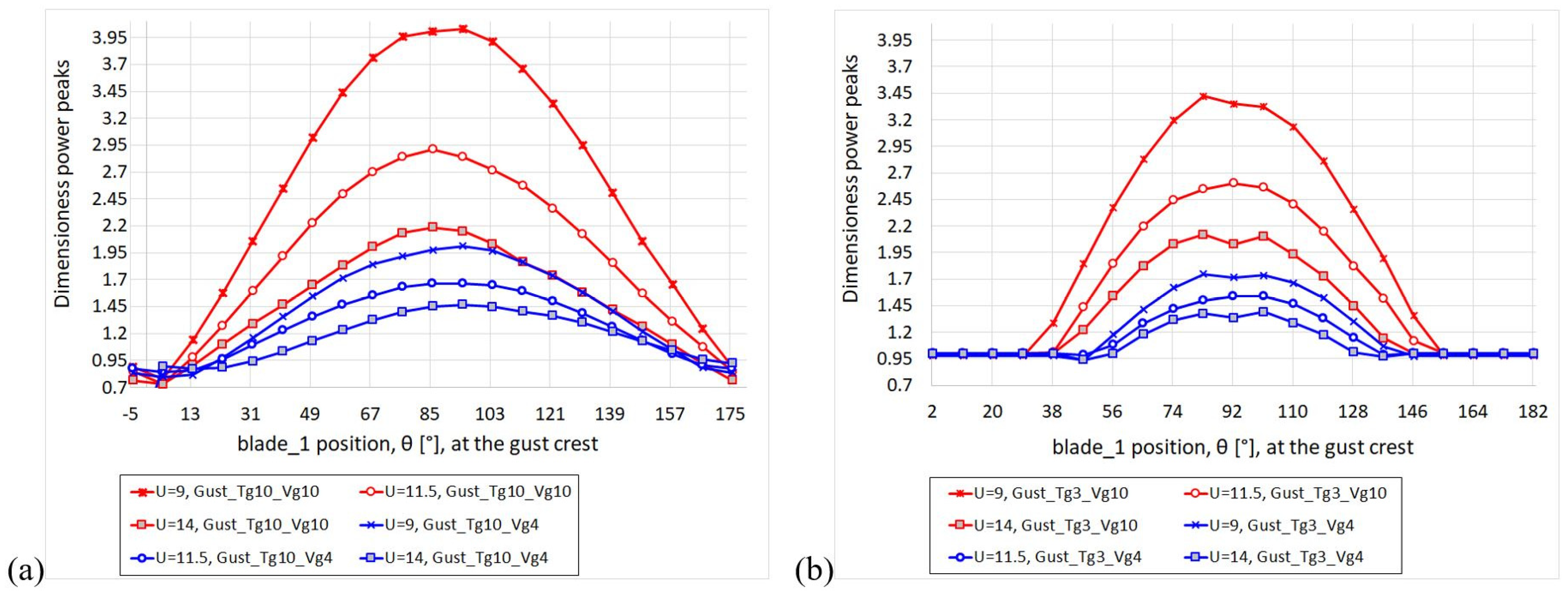
Figure 6 clearly shows the importance of the relative phase between the blades and the gust. It provides the power maximum peak during the gust (normalized by the peak calculated during a complete revolution of the corresponding steady wind case) as a function of the position of blade_1 at the gust crest, for different and gust types. Note that the overloads always occur when the blade is at about halfway upwind, and therefore the second blade is halfway downwind, at the instant the gust crest occurs. More precisely, when θ is 86 ÷ 95 in the case of = 10 s, and when θ is 83 ÷ 101 in the case of = 3 s. The gap visible in Figure 6b for θ < 30° and θ > 155° should not be surprising, since when these short gusts ( = 3 s) occur during the minimums of the fluctuating curve of the overload peaks cannot exceed those of the regular operation.
Figure 6.
Maximum power (divided by the steady condition maximum power) under gusts with period: (a) = 10 s; (b) = 3 s.
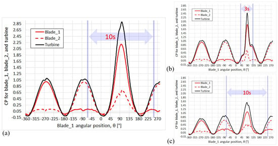
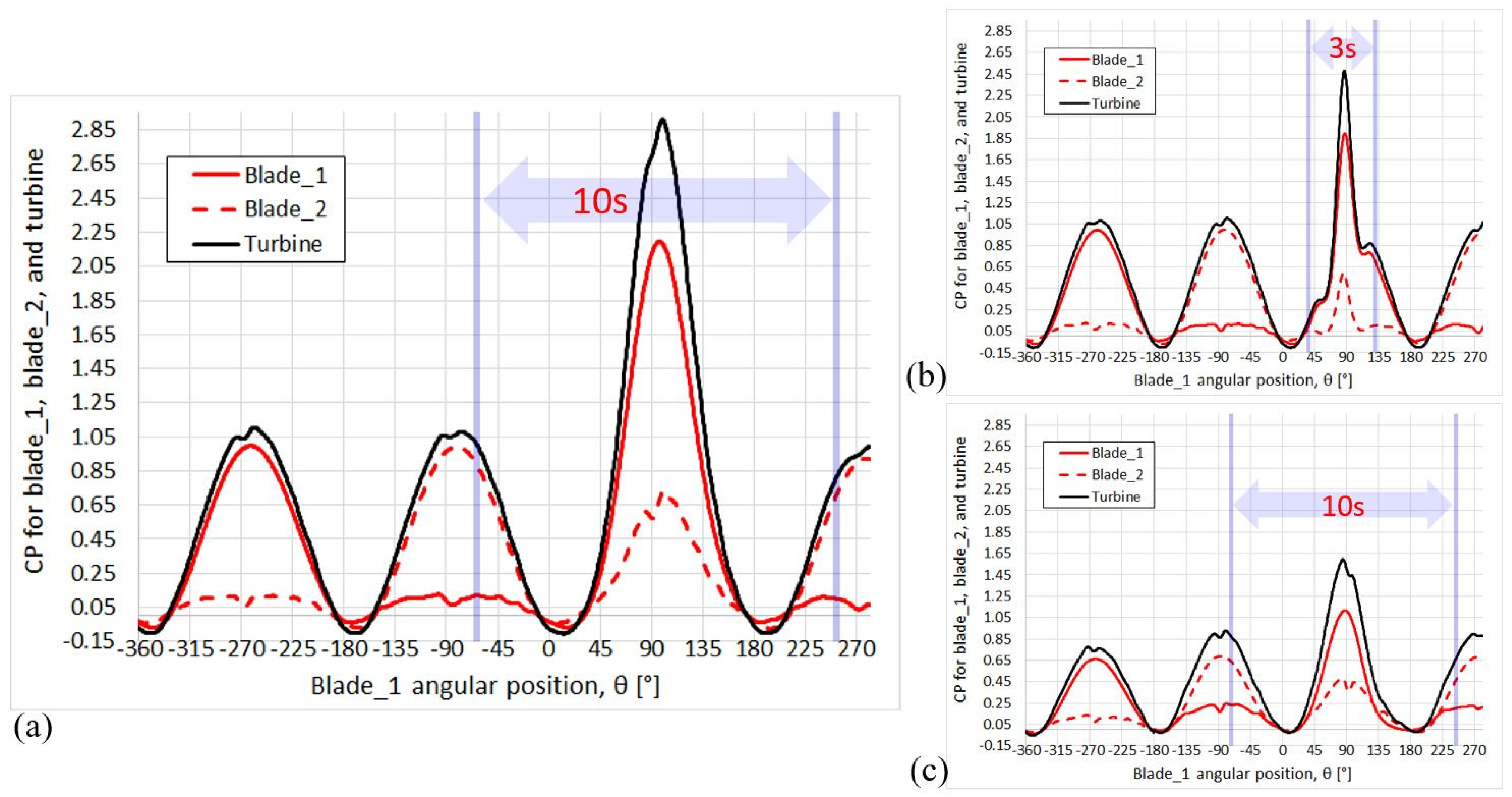
Figure 7 shows that the physical mechanism responsible for the severe overloads occurring when the blades are at half upwind and half downwind at the occurrence of the gust crest is a “constructive interference” of the of the individual blades. The phenomenon is particularly intense because our turbine is two-bladed. In fact, while in general for VAWTs each blade experiences maximum torque a first time when it is approximately halfway upwind and a second time when it is halfway downwind (see Figure 3b), only for turbines with two (or a multiple of two) blades does this happen at exactly the same time. Figure 7 illustrates three cases for which the maximum overload occurs.
Figure 7.
for: (a) = 9 m/s, = 10 s, = 6 m/s, θ = 95° at the gust crest; (b) = 9 m/s, = 3 s, = 6 m/s, θ = 83° at the gust crest; (c) = 14 m/s, = 10 s, = 6 m/s, θ = 86° at the gust crest.
Figure 7a,b show cases with the same and different ; the gust peak occurs when the blades are almost at the same azimuthal position, i.e., halfway upwind and halfway downwind. It can be seen that the overload peak depends little on ; in other words, within the investigated range of gust periods (from 3 to 10 s), a short period gust is almost as dangerous as a long period gust.
Comparing Figure 7a,c, illustrating cases that differ only in (same reasoning as above for θ at the gust crest occurring), it is noted that the overload peak for = 9 m/s is huge compared to that achieved for = 14 m/s. The main reason for this is the non-proportionality of with respect to ; in fact, in our analysis the values are the same regardless of , and consequently the relative effects of the gust are obviously much more intense in the lower case.
However, a further reason dampens the gust overload effect in the case = 14 m/s: the state of the fluid on the blade. In fact, while with = 9 m/s the flow is well attached, with = 14 m/s the flow is already partially stalled (see the streamlines in Figure 3b), hence a sudden availability of additional kinetic energy brings the blade very quickly into deep stall without it being able to generate very high extra power. This issue will be better deepened and discussed in the next section.
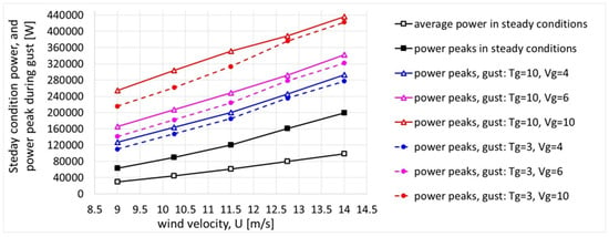
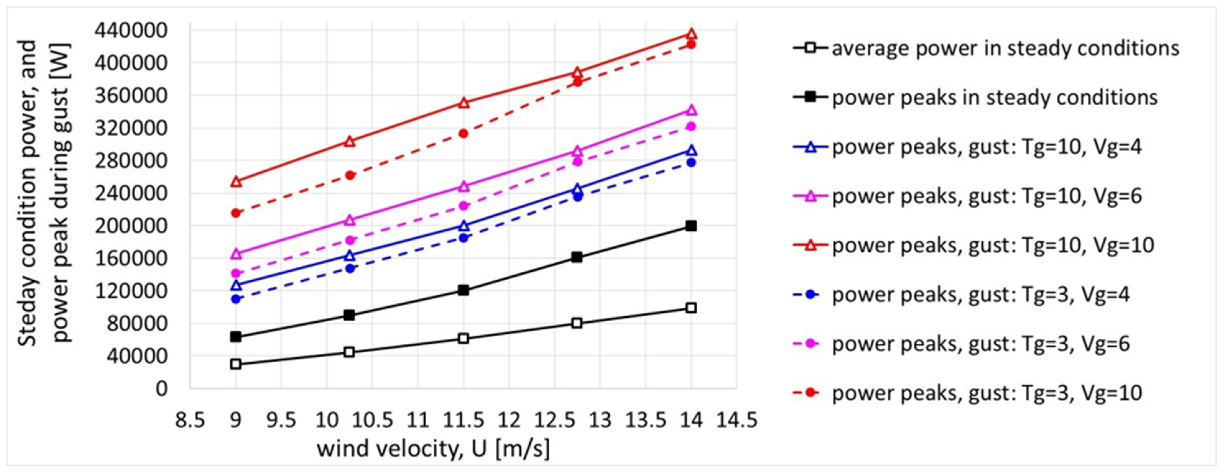
Figure 8 summarizes the results found for all the cases, in terms of maximum power peaks; for completeness, the average power and the peaks of the corresponding cases of steady wind are also reported. As noted above, it is trivial to reiterate that the effects of the gusts, relative to the stationary case, appear very large at = 9 m/s but fade as increases, mainly due to the lack of scaling of the gust amplitude as a function of .
Figure 8.
Average and maximum power at steady conditions, together with maximum power under gusty wind conditions (1 m of blades).
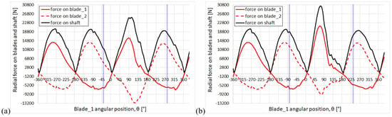
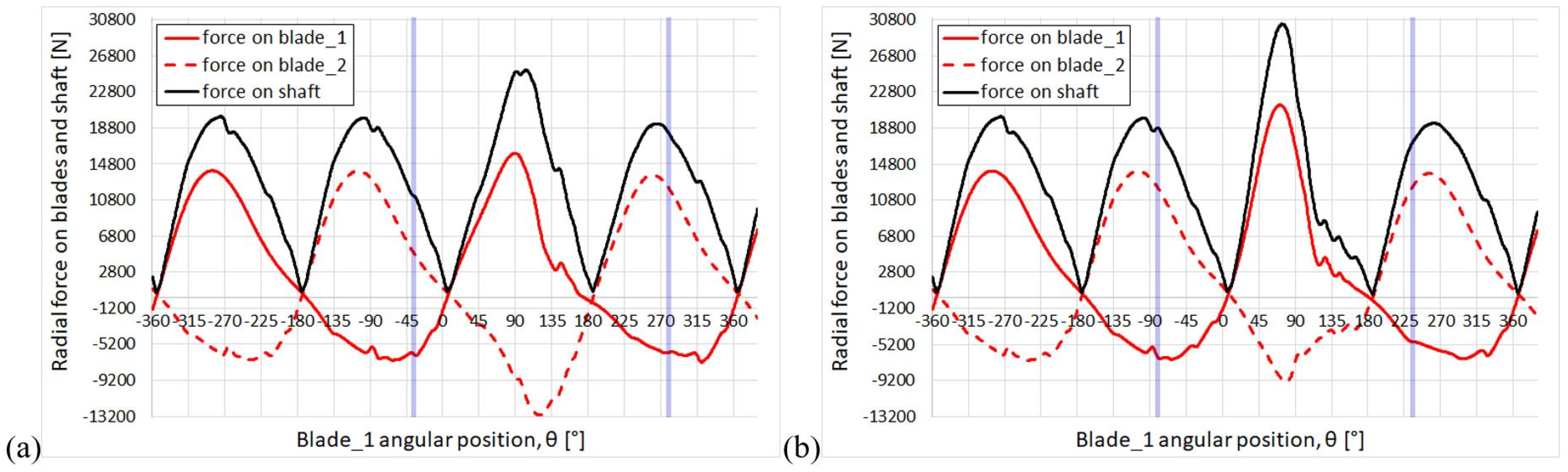
The next step of this analysis is to show the results obtained for the radial forces on blades and tower. As shown in Figure 9 for = 14 m/s, each blade experiences a positive radial force (compression) during upwind and a negative radial force (tension) during downwind; since the blades are radially aligned and the forces have the same orientation, the total force on the shaft is obtained by adding the magnitudes of the radial forces on the blades.
Figure 9.
Radial force on the blade and overall force on shaft (1 m of blades) under gusts with = 10 s and = 10 m/s: (a) θ = 122°; (b) θ = 77°.
In particular, Figure 9a,b illustrate respectively the most severe case for the tension peak (occurring when θ = 122° at the gust crest; note that the tension force is acting on blade_2) and the most severe case for the shaft force peak (when θ = 77° at the gust crest). For the force on the shaft, a constructive interference effect is again observed; in fact, the gust crest occurs nearly in conjunction with the blade angular position that provides both maximum compression and maximum tension.
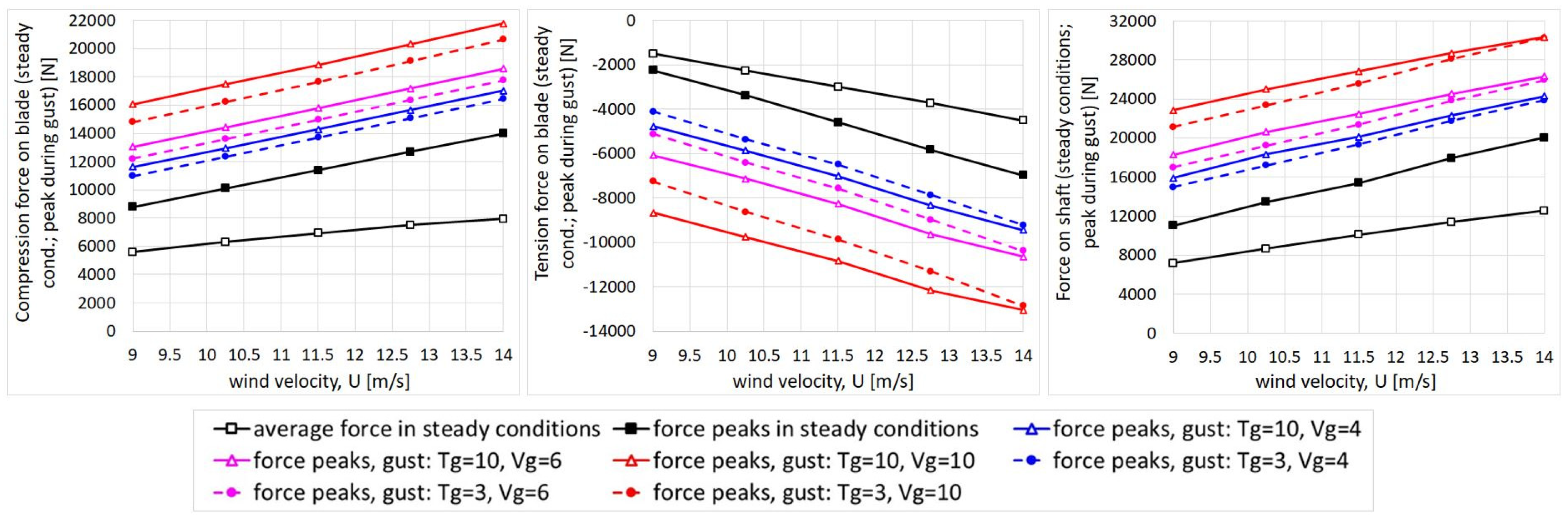
Figure 10 summarizes all the results concerning the radial overloads, compared to the respective cases without gusts. As expected, gusts prove to have a large effect on radial forces as well. For a given wind speed, the greater the gust amplitude, the greater the overload. Similar considerations to those already made for the power peaks can now be made regarding the radial force peaks, yet a further insight will be given in next section.
Figure 10.
Average and maximum radial forces at steady condition on blade and shaft, together with the max. forces in gusty winds (1 m of blades).
It is worth reiterating that Figure 8 and Figure 10 only show the maximum peaks, obtained under the most severe blade/gust phasing conditions. These conditions were identified by performing a series of simulations, each with a 9° step for each gusty wind operating condition (this means 20 simulations per operating condition; therefore, 1200 simulations were needed in total for this analysis, including some runs performed at = 55% and 70%, that will be discussed in the next section).
To conclude this section, we will quantify the most critical overloads predicted. Although the maximum relative overloads were found for the lowest steady-state wind speeds, the maximum absolute peaks were found for the case of the highest steady-state wind speed that was examined (14 m/s, nominal wind). Therefore, comparing the maximum peaks obtained with and without the gust, the most severe overloads were the following: +119% for power, +56%, and +87% for compressive and tensile forces on the blade and +51% for the force on the tower.
4. Discussion
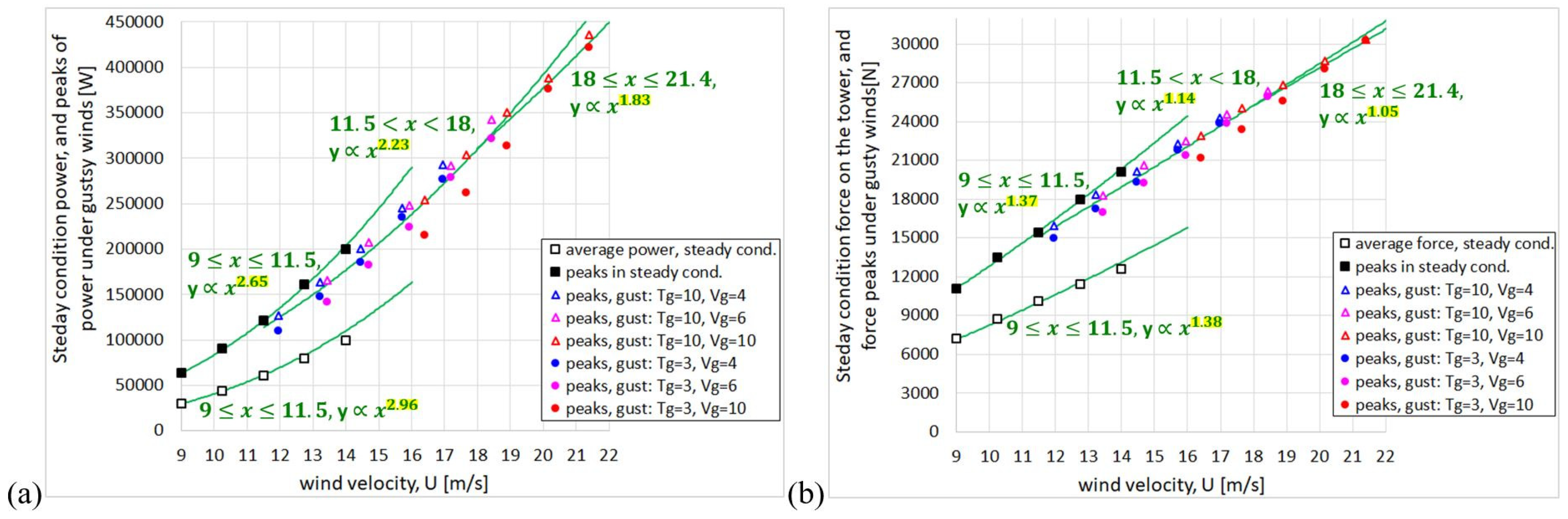
The purpose of the current section is to analyze the results without the bias implicit in the lack of proportionality of the gust amplitude with respect to the steady wind magnitude. To this end, the same results seen in Figure 8 and Figure 10 (only power and force on the tower, for briefly) have been rearranged in Figure 11, where the abscissa shows the steady wind speed or the maximum wind speed reached during the gust crest, depending on whether the results are related to cases without gust or to cases with gust, respectively. Then, the reader must pay attention to the contingent meaning of in the abscissa. In green, “power-law” trend lines have also been added, distinguishing three speed ranges: 9 ≤ ≤ 11.5; 11.5 < < 18; 18 ≤ < 21.4. Note that 21.4 m/s is the maximum instantaneous wind velocity reached during the most intense gust ( = 10 m/s) for a steady wind of 14 m/s.
Figure 11.
Average and max. power at steady conditions, together with max. power under gusty wind conditions (a); average and max. force on tower at steady conditions, together with max. force on tower under gusty wind conditions (b). Power and forces are for 1 m of blades. In abscissa of both the graphs: highest wind velocity during the revolution.
Figure 11a shows that the average power and the peaks of the cases without gust almost vary up to = 11.5; beyond this speed a certain decrease is observed, coherently with the fact that the turbine is stall-controlled. In the cases with gust, as increases the power peaks grow with a trend significantly less than the cubic one. In fact, the exponent of the power law gradually decreases as increases, the greater the ; it can be seen that for = 10 m/s the exponent makes the trend less than quadratic with . Considering that the flow on the blade is increasingly separated as increases and therefore as α increases, the reason for this “overloads dumping” is the dramatic increase in the drag due to deep stall.
This phenomenon is detailed in the Appendix B, where the reader can find graphical explanations of how the lift and drag forces on the blade, and their projections in the directions of the blade motion and in the radial direction, vary as the wind speed increases (even instantaneously, during a gust) while the turbine’s rotation speed remains constant.
Focusing on the force on the shaft, Figure 11b shows that under stationary winds the average force and the peaks grow with a law that is halfway between linear and quadratic with U. This trend appears to be dampened under gusty winds, and also in this case the more the higher the Vg is. The mechanism that seems to protect the system from massive radial overloads in gusty conditions could be the progressive rotation of the aerodynamic force vector towards the tangential direction (thus, away from the radial direction) as increases and therefore as α increases, as illustrated in Appendix B. As a consequence, in the case of gust with = 10 m/s the force on the tower grows just linearly with .
Both overloads damping mechanisms, the growth of drag and the rotation of aerodynamic force, are consequences of the method of load regulation by passive stall, i.e., keeping constant at high wind speeds.
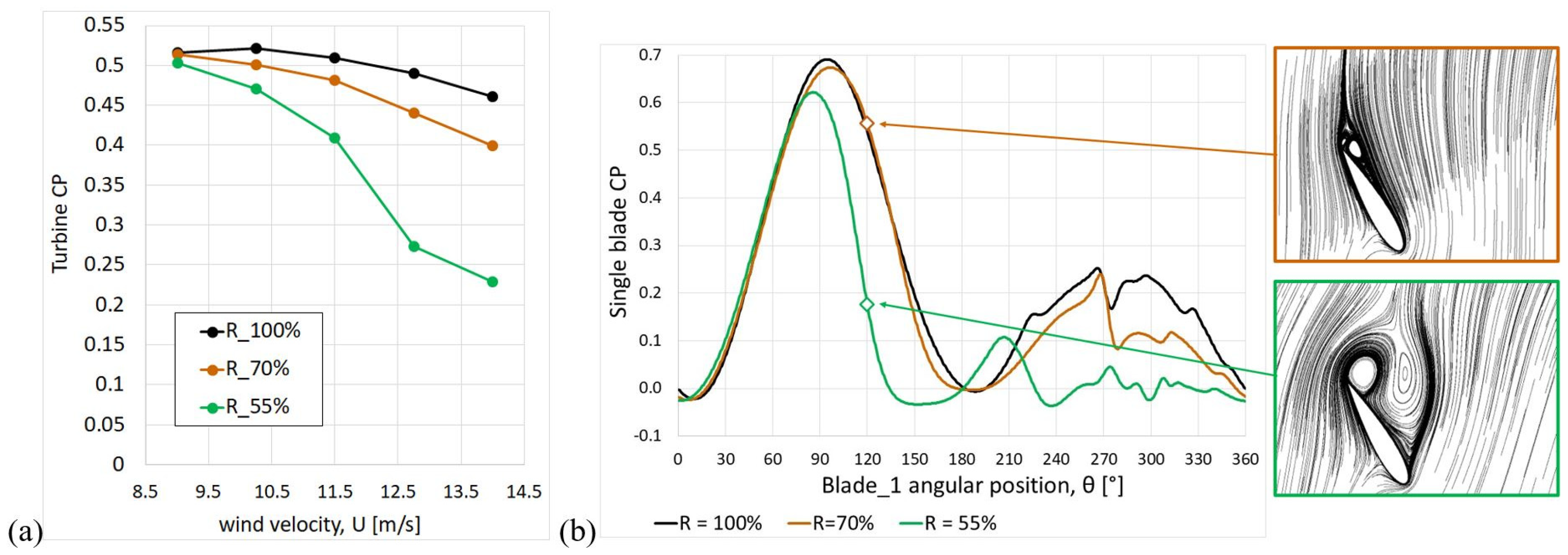
The final issue we will address is the potential concern for readers that our entire analysis is based on the equatorial plane of the turbine. In other words, what would happen to sections of the blade with a lower radius in gust conditions, given the blades’ particular shape (troposkein)? In order to dispel this doubt, further simulations were made at radii corresponding to 70% and 55% of the equatorial one, both in stationary conditions and in the presence of gusts. Figure 12a shows the of the turbine at maximum radii (equatorial), 70% and 55%, as a function of wind speed, . It is observed that, while at = 9 m/s the s differ only slightly, as increases the drops more rapidly the smaller the radius considered. To justify these results, it should be remembered that the blade chord is uniform in the spanwise direction and consequently the local “solidity” (sum of the chords/circumference) increases as the radius decreases; moreover, it is well known that turbines characterized by high solidity have low optimal TSRs and are characterized by a narrow -TSR curve, i.e., with performance that deteriorates rapidly as the TSR moves away from the optimal value [23]. However, it should also be considered that in the troposkein turbine, as the radius decreases, the local TSR also decreases and this avoids a significant decline in performance compared to the equatorial plane. However, Figure 12a shows that this only happens at = 9 m/s, whereas as increases, the blade stalls more rapidly the greater the solidity, i.e., the smaller the radius. The reason is well visible in Figure 12b, which compares the of the single blade at = 14 m/s; note that at θ = 120° the flow is very separated in the case of = 55% (see the streamlines inside the boxes).
Figure 12.
Turbine predicted at various radii (a); instantaneous blade during a revolution predicted at various radii, and flow details at θ = 120° (b).
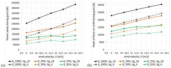
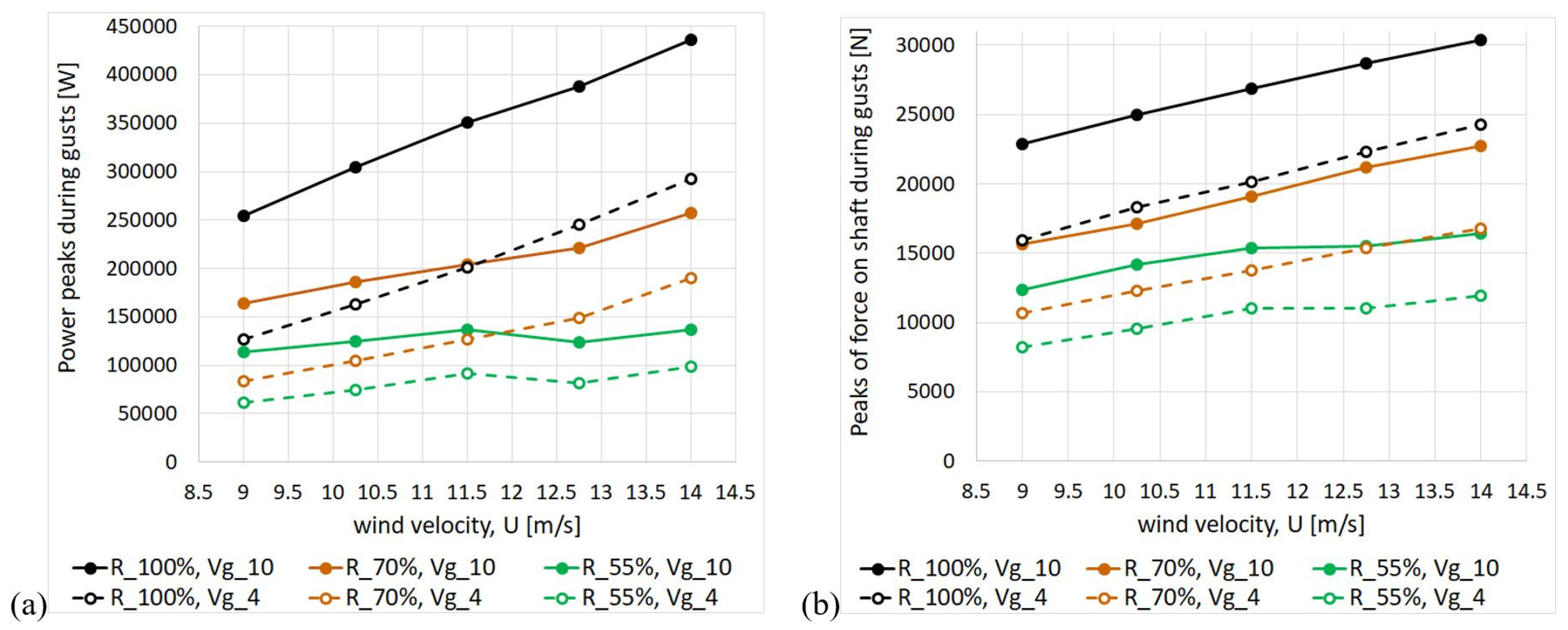
This proves that any increase in speed induces stall more rapidly the smaller the radius of the blade element. Some simulations were performed for = 70% and 55% under gusts with = 10 s and = 4 and 10 m/s. The maximum peaks of power and force on the shaft are shown in Figure 13 in comparison to the corresponding results already achieved at = 100%. It is interesting to note that for = 55% the peaks grow only weakly up to = 11.5 m/s, and that for higher they stop growing. We can conclude that the protective mechanism of damping the aerodynamic loads, due to the intensification of the stall, is even more effective at radii smaller than the equatorial one. compressive and tensile forces on the blade, and +51% for the force on the tower.
Figure 13.
Maximum power peaks under gusty wind conditions (1 m of blades) predicted at = 70% and 55% in comparison to = 100% (a); maximum peaks of force on the tower under gusty winds (1 m of blades) predicted at = 70% and 55% in comparison to = 100% (b).
One criticism of this work is that it is limited to a 2D analysis and that no conclusions can be drawn about the behavior of the entire turbine. Even if single simulations were performed at radii equal to 70% and 55% of the equatorial one, they would still be 2D simulations that cannot capture 3D effects. The most significant 3D effects of a vertical-axis turbine are typically the tip vortex and vertical flow divergence. These flows are also shown in 3D blade-resolved CFD simulations by Franchina et al. [25]. However, the tip vortices are less critical in the case of troposkein-shaped turbines: as Persico et al. [26] highlight, at low TSR, the troposkein-shape turbine is characterized by smaller and less persistent vortices compared to a H-blade turbine. Furthermore, the central part of the turbine is the main contributor to the torque. In Franchina et al. [27], an interesting comparison is made between a symmetric airfoil and a cambered one for a troposkein-shaped turbine. The torque coefficient trend is shown at different sections of the blade: it is clear that the central part makes the main contribution, while the flow is more separated towards the tips, a consequence of the reduced relative velocity and hence reduced local TSR.
A sudden increase in the freestream velocity during a gust causes the turbine to operate at a TSR that is lower than the optimal one (since remains constant). What should happen to the entire turbine? We cannot say for certain, but we can use the experimental data reported in [28] for a straight-blade turbine as a guide. In that case, several measurements were performed at different values (40, 50, and 65 rpm), and for each of these, different TSRs are shown (i.e., those obtained with a different freestream velocity and constant ). While the normal force coefficient is reported in the paper, it is easy to calculate the peak value of the normal force. Reducing the TSR is found to increase the normal force, but this effect is progressively dampened.
Tong et al. [29], shows possible 3D effects in straight-blade turbines that induce an increase in towards the tip at low TSR. However, experimental results in [28] show a dampened increase in the forces acting on the turbine as the freestream velocity increases, despite the possible 3D effects that could enhance the power coefficient towards the tip, shown by [29].
Another important experimental study is that of Fusetti et al. [30], in which a troposkein-shaped turbine was analyzed. In this study, the thrust coefficient of the turbine was measured at three different values (240, 300, and 320 rpm), each at different TSRs. By manipulating the data, we can determine the thrust force as a function of the freestream velocity. As in the previous experimental case, a dampened increase in forces is visible as the freestream velocity increases.
Therefore, since most of the troposkein-shaped turbine production is located in the central part and some experimental studies show a dampened increase in forces when reducing the TSR (operating at constant ), it seems reasonable to hypothesise the same qualitative behaviour for the entire turbine as that analysed for the 2D section during the gust. However, the issue remains open and future experimental or 3D blade-resolved studies will be required at low TSR to provide clarification.
5. Conclusions
The transient loads of a stall-controlled vertical-axis wind turbine are analyzed under extreme gusty wind conditions with gust amplitudes ranging from 4 to 10 m/s. The 2D-CFD simulations are performed for the equatorial plane of the turbine (where the radius is maximum), since the power output is maximum in the central band, where the frontal area is largest. Comparing the highest peaks to the peaks of the no-gust nominal wind condition, the most severe instantaneous overloads were the following: +119% for power, +56% and +87% for compressive and tensile forces on the blade, and +51% for the force on the tower. Please note that these results are specific to the equatorial plane and not the entire turbine. It is worth mentioning some observations.
- -
- The overloads depend on the gust amplitude but depend little on the gust duration within the investigated range of periods (), showing that a 3 s gust can be almost as dangerous as a 10 s one.
- -
- The highest overloads of power and tower force are generated by a constructive interference mechanism of the contributions of each blade, which is possible when the angular position of the blades in conjunction with the crest of the gust is about the same that would produce the maximum force on the individual blade during the revolution. The effect is maximized by the considered geometry, since the turbine has only two blades.
- -
- Maintaining a fixed turbine speed (stall-regulation method) could have advantages during gusts, as it could dampen both excessive power overloads (thanks to the increase in aerodynamic drag) and excessive radial force overloads (thanks to the rotation of the vector of the aerodynamic resultant force on the blade, towards the tangential direction).
To conclude, it is important to reiterate that other CFD methods (low-orders hybrid methods) are preferable, from an engineering point of view, to the one used in the present analysis whose aim was not only to investigate the fundamental fluid–blade interaction mechanisms occurring during the gust but also to provide (high-fidelity) accurate comparison data that may be useful in the future to calibrate more efficient (as they require low computation times) hybrid CFD models.
Author Contributions
Conceptualization, S.Z.; methodology, S.Z. and M.P.; validation, S.Z.; formal analysis, S.Z.; investigation, M.P.; Data curation, M.P.; writing—original draft preparation, S.Z.; writing—review and editing, M.P.; supervision, S.Z.; funding acquisition, S.Z. All authors have read and agreed to the published version of the manuscript.
Funding
This research was funded by National Recovery and Resilience Plan (NRRP), CN1, Centro Nazionale di Ricerca in High Performance Computing, Big Data e Quantum Computing, spoke 6: multiscale modelling & engineering applications.
Institutional Review Board Statement
Not applicable.
Informed Consent Statement
Not applicable.
Data Availability Statement
The original contributions presented in this study are included in the article. Further inquiries can be directed to the corresponding author.
Conflicts of Interest
The authors declare no conflict of interest.
Appendix A. Grid Sensitivity Analysis and Model Validation
A well-known test case from the technical literature, the SANDIA National Laboratories 17 m VAWT [31], was adopted for the sensitivity analysis to grid refinement and the validation of the numerical model. The turbine has two troposkein-shaped blades with NACA 0015 airfoil and chord length of 0.61 m. This is one of the rare cases of a significant size turbine being tested in an open field. The aerodynamic forces acting on the individual blade are derived from pressure measurements detected by pressure transducers placed all around the blade profile at the equatorial plane of the turbine only. This peculiarity makes the data from their experimental campaign useful for validating CFD models, even 2D ones. The rotation speed is fixed at 38.7 rpm (revs per minute) for the local force measurements, and at 42.2 rpm for the classical measurement. The dimensions of the calculation domain, in relation to the turbine diameter, are the same as those adopted for the 5 MW turbine which is the subject of this article. Are they sufficient to avoid any blockage effect? The answer of course is no since, as demonstrated in [32] for the CFD 2D of a tidal VAWT: the turbine efficiency continues to decrease both as the upwind distance between the domain entrance and the turbine increases, and as the crosswise width of the domain increases, albeit with an asymptotic trend. In particular, Ref. [32] shows that an upwind distance of 7∗D leads to an overestimation of the by 5% compared to a distance of 108∗D, and that a width of 20∗D leads to an overestimation of the by 6% compared to a width of 150∗D. Due to the exorbitant number of simulations performed for this study, the above approximations were deemed acceptable in order to save computational time. To investigate the effects of grid refinement in the blade region, four grids, designated A, B, C, and D, were generated for the rotating grid including the blades. As summarized in Table A1, the varied parameters are number of nodes on the periphery of the rotating grid; number of nodes on the blade profile; height of the first cell at the blade wall; and number of layers of regular quad cells enveloping the blade. It can be noted that from the finest grid (A) to the coarsest grid (D) the average value of y+ varies from 0.04 to 2.8.
Table A1.
Grid refinements.
Figure A1 shows the comparison between our CFD results and experimental results [31] in terms of tangential and radial (or normal) coefficients, and , defined as
where Ft and Fr are tangential and radial forces for unit of span, respectively; the apparent speed is calculated as vector sum of freestream wind speed and the blade speed. Two TSRs are considered: 4.6, which is in the range of optimal values, i.e., which lead to maximum , and 2.33, which is instead representative of a deep stall condition. It should be emphasized that since the experimental measurements are local (on the almost straight section of the blade, at the equatorial plane of rotor) the differences with the 2D CFD should be limited, although local three-dimensional fluid dynamic effects are unavoidable. It can be seen that the 2D CFD model fits, at least qualitatively, the main characteristics of the and experimental curves in a sufficiently passable way, for both the TSR values. Regarding the effect of grid resolution in the blade region, it is interesting to note that the finer the grid, the greater the tangential force (and hence the torque), as already evidenced in a previous study [33]. This is attributable to fine grids’ greater ability to accurately simulate the transition from attached to detached flow states. Coarsen grids lead to an earlier (and excessive) flow separation, as evidenced by the fact that the largest difference in the curve between fine grids (A, B) and coarse grids (C, D) is evident in the case of TSR = 2.33 (deep stall). Since the differences between the results of grids A and B are small, in order to save computation time, it was decided to adopt grid B also for the 5 MW turbine.
Figure A1.
Blade and obtained at TRS 4.6 (a,b) and at TSR 2.33 (c,d) for the grids of Table A1, in comparison to the experimental values detected for the blade section at the equatorial plane of the rotor [31].
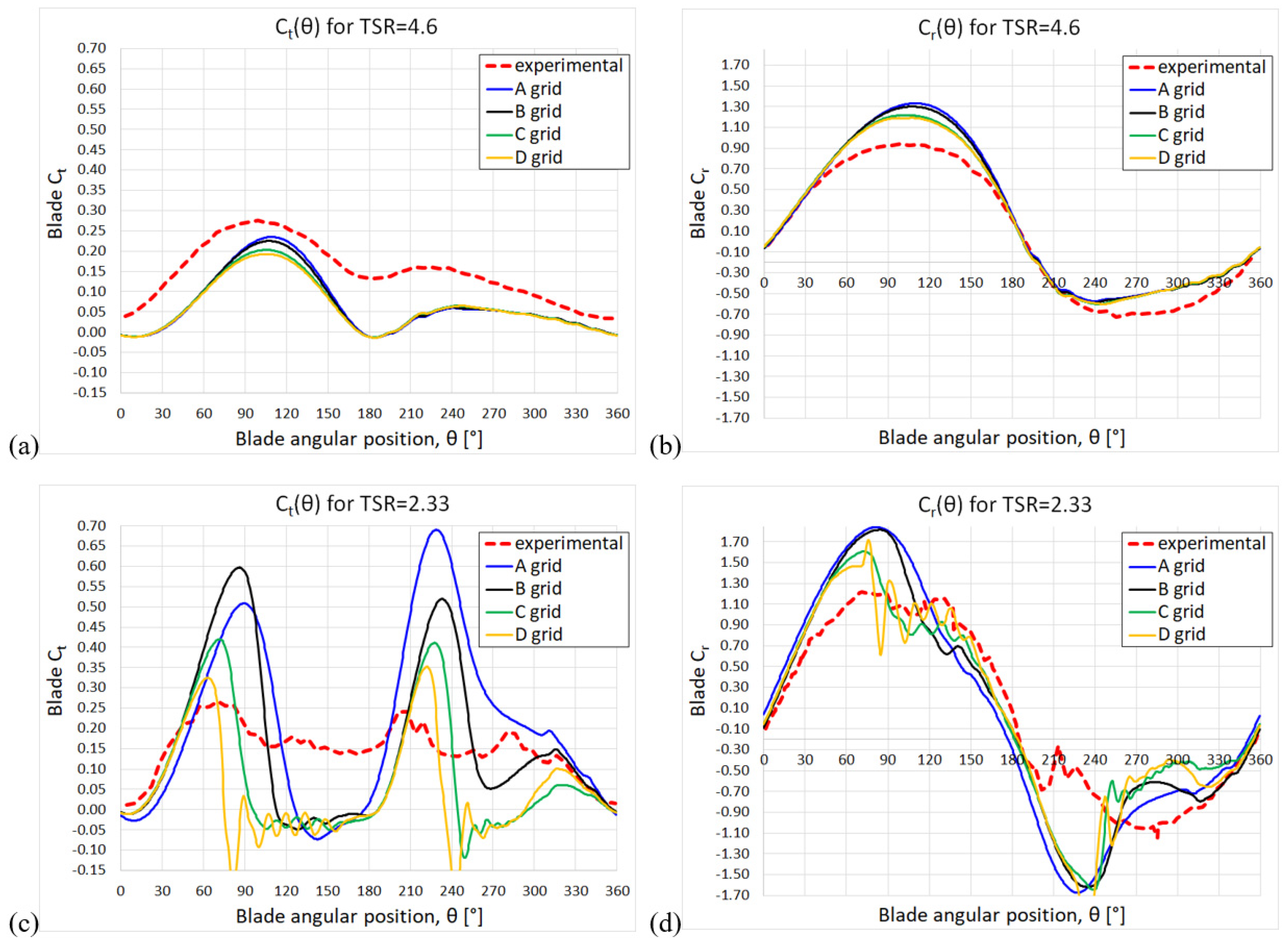
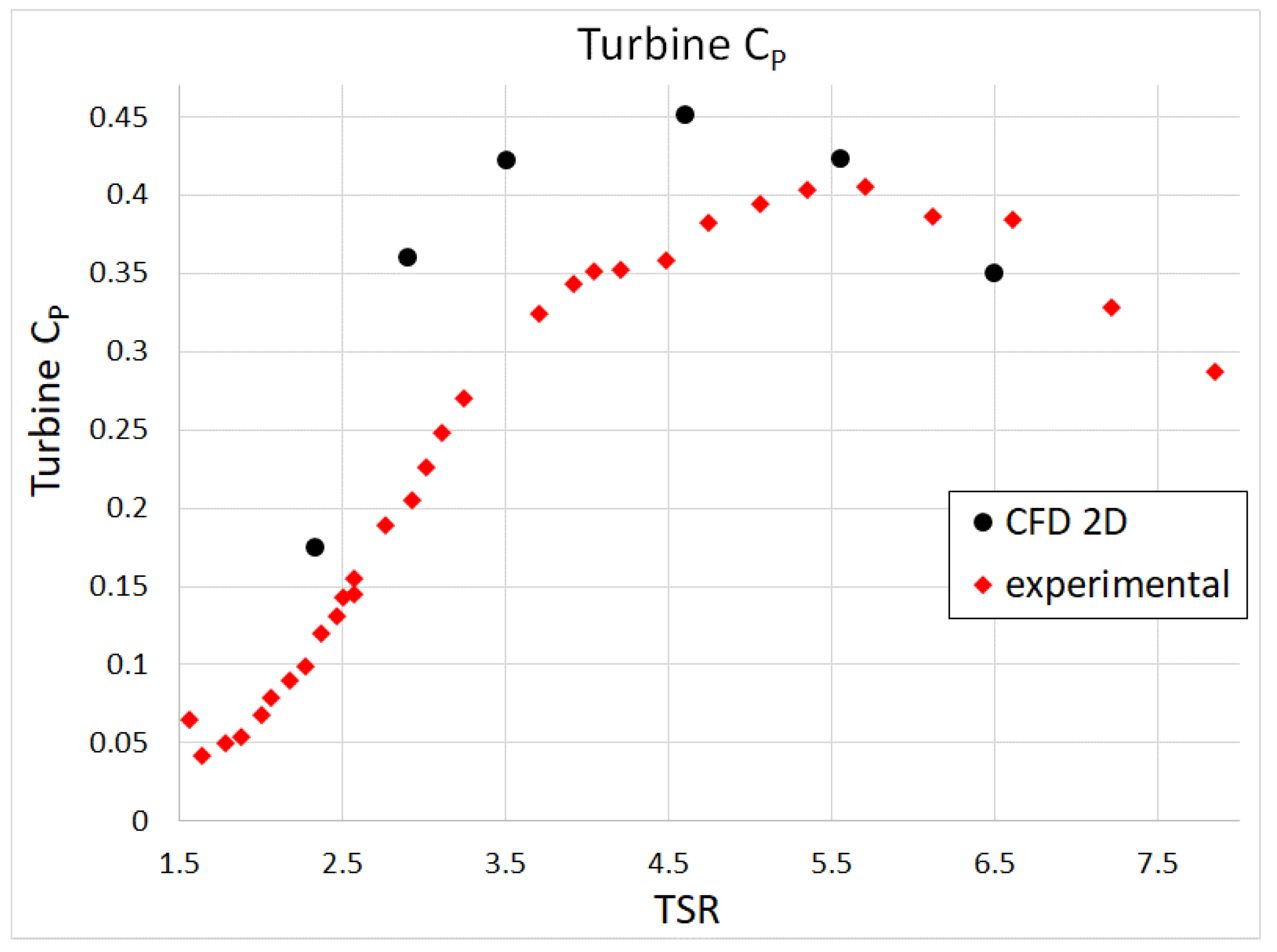
Figure A2 shows the turbine as a function of TSR. As expected, the 2D CFD overestimates the experimental values. This is due to the fact that the troposkein turbine is characterized by an efficiency drop from the central (equatorial) section towards the blade tips, mainly due to the occurrence of non-optimal local TSR values as the local turbine radius decreases.
Figure A2.
Turbine as a function of TSR obtained by our CFD 2D model in comparison to the experimental turbine [31].
Appendix B. Forces on the Blade as the Wind Speed Varies
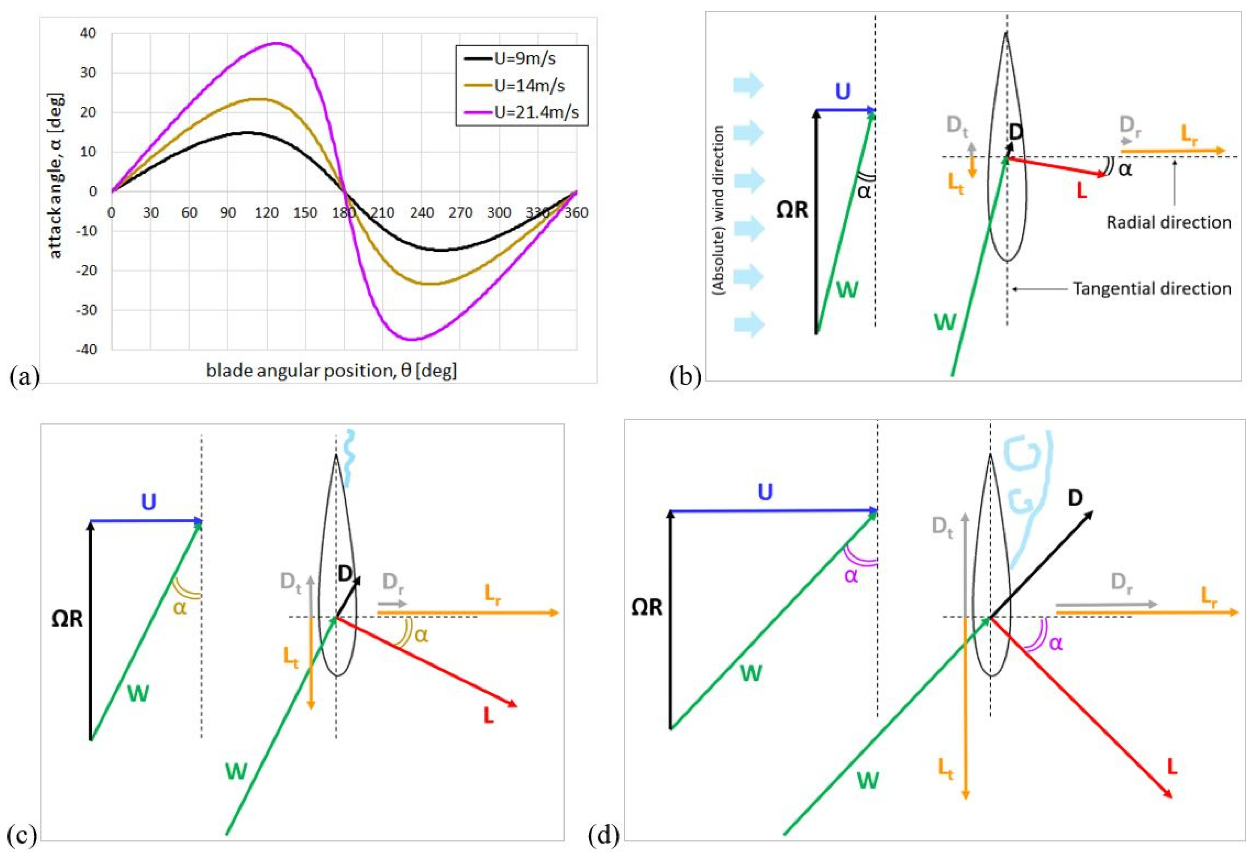
This section gives qualitative explanations on what happens to the forces generated on the blade when the wind speed increases and the turbine rotation speed, , is kept fixed. The following considerations are based on the velocity triangles, the vectors of the forces exerted by the fluid on the blade, and trends, well known from the experimental literature, of the lift and drag coefficients as a function of the angle of attack. Figure A3a shows the evolution of the attack angle, α, during a revolution at different wind speeds: = 9 (rated wind speed), 14 m/s, and 21.4 m/s. As already mentioned, the last value corresponds to the maximum wind speed reached during a gust with Vg = 10 m/s occurring when = 14 m/s. The curves in the graph were obtained simply on the basis of trigonometry, having neglected that the fluid when it reaches the blade should already be slowed down respect to the freestream speed. This simple representation captures two fundamental aspects: the maximum α occurs not far from upwind and downwind halfway point; the maximum α increases significantly as the wind speed increases. It should be stressed that the value of α is crucial since it determines the lift and drag coefficients, and :
where and are the lift and drag forces per unit of blade span. Consistently with Equation (A2), it can be written that
It is useful to remember how the and projections generate tangential force, Ft, and therefore torque, M:
and the radial force, Fr:
Figure A3b–d illustrate the velocity triangles ( is the blade speed, which is the same in the three cases since is fixed) and the and vectors, together with their projections in the direction of the blade motion (tangential direction) and in the radial direction, as the wind speed increases, and therefore as α increases.
A basic concept of fluid dynamics is that in the “pre-stall region” (i.e., for small-moderate α) increases ∝ α, while remains very small (~1/100 of ). In Figure A3b we illustrate a condition for which the flow is attached, / is maximum and therefore the turbine efficiency, , is maximum, as in particular it happens for = 9 m/s. However, this figure could be representative of what happens with any lower wind speed, since up to 9 m/s is regulated ∝ to keep the at its maximum, and therefore the similarity is preserved for the velocity triangle, i.e., α is constant; as a consequence, and depend only on and then vary ∝ , while the turbine power, , varies ∝ .
Figure A3c shows a case of slight flow separation due to an increase in α, as could happen for = 14 m/s having kept fixed. Despite the increase in drag, lift remains the dominant force as continues to grow, albeit less than linearly with α. Power output continues to grow with less than cubically, so does not drop considerably, mainly due to the rotation of the vector towards the tangential direction. A further growth of α leads to stall, as depicted in Figure A3d, representative of the condition = 21.4 m/s. This represents the “post-stall region” (i.e., large α), where stops growing and begins to decline, while increases rapidly and significantly. It can be noted that the rotation of the vector , in the direction of producing torque, is even more accentuated and also the magnitude of is still greater than the magnitude of ; consequently, continues to grow, but much less than ∝ because of a massive drag increase. This effect, i.e., the decrease in , is the desired phenomenon in any load regulation method, with the difference that while in horizontal axis turbines it is obtained by considerably reducing the angle of attack (by regulating the pitching angle of the blade), in vertical-axis turbines it is obtained by letting the blade stall.
We conclude this section by examining what happens to the radial force as α increases (Figure A3b–d). The growth of with appears damped for > 9 m/s, whereas for lower than the rated speed goes approximately ∝ (as can be deduced from Equations (A3) and (A5)). The main reason for this slowdown is the above-mentioned rotation of the vector , which implies the decrease (relative to the current value of the magnitude of ) of the projection of in the radial direction.
Figure A3.
Evolution of α during a revolution, for different wind velocities (a); velocity triangle and vectors of the forces (together their projections) for increasing wind velocities, keeping fixed (b–d).
References
- Danao, L.A.; Eboibi, O.; Howell, R. An experimental investigation into the influence of unsteady wind on the performance of a vertical axis wind turbine. Appl. Energy 2013, 107, 403–411. [Google Scholar] [CrossRef] [Scilit]
- Shahzad, A.; Asim, T.; Mishra, R.; Paris, A. Performance of a vertical axis wind turbine under accelerating and decelerating flows. Procedia CIRP 2013, 11, 311–316. [Google Scholar] [CrossRef] [Scilit]
- Battisti, L.; Benini, E.; Brighenti, A.; Soraperra, G.; Castelli, M.R. Simulating the dynamic behavior of a vertical axis wind turbine operating in unsteady conditions. J. Phys. Conf. Ser. 2016, 753, 022002. [Google Scholar] [CrossRef] [Scilit]
- Yu, H.; Shao, M.; Miang, H. Numerical study on the time-harmonic gust response of a vertical axis wind turbine. Phys. Fluids 2025, 37, 015109. [Google Scholar] [CrossRef] [Scilit]
- Wu, Z.; Bangga, G.; Cao, Y. Effects of lateral wind gusts on vertical axis wind turbines. Energy 2019, 167, 1212–1223. [Google Scholar] [CrossRef] [Scilit]
- Danao, L.A.; Edwards, J.; Eboibi, O.; Howell, R. A numerical investigation into the influence of unsteady wind on the performance and aerodynamics of a vertical axis wind turbine. Appl. Energy 2014, 116, 111–124. [Google Scholar] [CrossRef] [Scilit]
- Bhargav, M.; Kishore, V.R.; Laxman, V. Influence of fluctuating wind conditions on vertical axis wind turbine using a three dimensional CFD model. J. Wind Eng. Ind. Aerodyn. 2016, 158, 98–108. [Google Scholar] [CrossRef] [Scilit]
- Wekesa, D.W.; Wang, C.; Wei, Y.; Danao, L.A. Analytical and numerical investigation of unsteady wind for enhanced energy capture in a fluctuating free-stream. Energy 2017, 121, 854–864. [Google Scholar] [CrossRef] [Scilit]
- Onol, A.O.; Yesilyurt, S. Effects of wind gusts on a vertical axis wind turbine with high solidity. J. Wind Eng. Ind. Aerodyn. 2017, 162, 1–11. [Google Scholar] [CrossRef] [Scilit]
- Srinivasan, L.; Ram, N.; Rengarajan, S.B.; Mohammad, A.; Divakaran, U.; Velamati, R.K. Effect of Macroscopic Turbulent Gust on the Aerodynamic Performance of Vertical Axis Wind Turbine. Energies 2023, 16, 2250. [Google Scholar] [CrossRef] [Scilit]
- Rakib, M.I.; Evans, S.P.; Clausen, P.D. Measured gust events in the urban environment, a comparison with the IEC standard. Renew. Energy 2020, 146, 1134–1142. [Google Scholar] [CrossRef] [Scilit]
- Padron, A.S.; Alonso, J.J.; Palacios, F.; Barone, M.; Eldred, M.S. Multi-fidelity uncertainty quantification: Application to a vertical axis wind turbine under an extreme gust. In Proceedings of the 15th AIAA/ISSMO Multidisciplinary Analysis and Optimization Conference (AIAA AVIATION 2014), Atlanta, GA, USA, 16–20 June 2014. [Google Scholar]
- Kjellin, J.; Eriksson, S.; Bernhoff, H. Electric Control Substituting Pitch Control for Large Wind Turbines. J. Wind Energy 2013, 2013, 342061. [Google Scholar] [CrossRef] [Scilit]
- Toor, Z.; Bahaidarah, H.M.; Zayed, M.E. Research on aerodynamic performances of the vertical-axis wind turbines under different wind gust configurations: Comparative numerical modeling. Multiscale Multidiscip. Model. Exp. Des. 2026, 9, 99. [Google Scholar] [CrossRef] [Scilit]
- Ran, Z.; Miao, W.; Lai, Y.; Pan, Y.; Ou, H.; Zhang, R. Parameter Optimization Design of Adaptive Flaps for Vertical Axis Wind Turbines. Energies 2025, 18, 4333. [Google Scholar] [CrossRef] [Scilit]
- Zhang, W.; Liu, Y.; Chen, C.; Yao, Z.; Teng, Y.; Li, X. Effects of wind gusts on the aerodynamic performance of a vertical-axis wind turbine with variable pitch. AIP Adv. 2026, 16, 045106. [Google Scholar] [CrossRef] [Scilit]
- Moore, K.R.; Ennis, B.L. Vertical-axis wind turbine steady and unsteady aerodynamics for curved deforming blades. AIAA J. 2022, 60, 189–196. [Google Scholar] [CrossRef] [Scilit]
- Rocchio, B.; Deluca, S.; Salvetti, M.V.; Zanforlin, S. Development of a BEM-CFD tool for Vertical Axis Wind Turbines based on the Actuator Disk model. Energy Procedia 2018, 148, 1010–1017. [Google Scholar] [CrossRef] [Scilit]
- Vita, L. Offshore Vertical Axis Wind Turbine with Floating and Rotating Foundation. Ph.D. Thesis, Technical University of Denmark, Lyngby, Denmark, 2011. [Google Scholar]
- Menter, F.R. Zonal two equation k-ω turbulence models for aerodynamic flows. In Proceedings of the 23rd Fluid Dynamics, Plasmadynamics, and Lasers Conference, Orlando, FL, USA, 6–9 July 1993. AIAA-93-2906. [Google Scholar]
- Menter, F.R. Two-equation eddy-viscosity turbulence models for engineering applications. AIAA J. 1994, 32, 1598–1605. [Google Scholar] [CrossRef] [Scilit] [PubMed]
- Orlandi, A.; Collu, M.; Zanforlin, S.; Shires, A. 3D URANS analysis of a vertical axis wind turbine in skewed flows. J. Wind Eng. Ind. Aerodyn. 2015, 147, 77–85. [Google Scholar] [CrossRef] [Scilit]
- Burton, T.; Jenkins, N.; Sharpe, D.; Bossanyi, E. Wind Energy Handbook, 2nd ed.; John Wiley & Sons Ltd.: Chichester, UK, 2011. [Google Scholar]
- IEC 61400-1; Wind Turbines—Part 1: Design Requirements. International Electrotechnical Commission: Geneva, Switzerland, 2005.
- Franchina, N.; Kouaissah, O.; Persico, G.; Savini, M. Three-dimensional modeling and investigation of the flow around a troposkein vertical axis wind turbine at different operating conditions. Renew. Energy 2022, 199, 368–381. [Google Scholar] [CrossRef] [Scilit]
- Persico, G.; Dossena, V.; Paradiso, B.; Battisti, L.; Brighenti, A.; Benini, E. Three-dimensional character of VAWT wakes: An experimental investigation for h-shaped and Troposkien architectures. In Proceedings of the ASME Turbo Expo 2016: Turbomachinery Technical Conference and Exposition, Seoul, Republic of Korea, 13–17 June 2016; ASME: New York, NY, USA, 2016; Volume 49873, p. V009T46A015. [Google Scholar]
- Franchina, N.; Kouaissah, O.; Barigozzi, G.; Persico, G. Sensitivity of Vertical Axis Wind Turbines to Rotor Shape and Blade Design: A Computational Investigation. In Proceedings of the 15th European Conference on Turbomachinery Fluid Dynamics and Thermodynamics (ETC 2023), Budapest, Hungary, 24–28 April 2023; pp. 1–15. [Google Scholar]
- Dyachuk, E.; Rossander, M.; Goude, A.; Bernhoff, H. Measurements of the aerodynamic normal forces on a 12-kW straight-bladed vertical axis wind turbine. Energies 2015, 8, 8482–8496. [Google Scholar] [CrossRef] [Scilit]
- Tong, G.; Yang, S.; Li, Y.; Feng, F. Effects of blade tip flow on aerodynamic characteristics of straight-bladed vertical axis wind turbines. Energy 2023, 283, 129105. [Google Scholar] [CrossRef] [Scilit]
- Fusetti, A.; Tomassoni, C.; Sanvito, A.G.; Mora, A.; Crema, D.; Gobbi, M.; Dossena, V. Design and commissioning of the laboratory-scaled model of a Troposkein VAWT for floating offshore applications. J. Phys. Conf. Ser. 2026, 3224, 092027. [Google Scholar] [CrossRef] [Scilit]
- Akins, R.E. Measurement of Surface Pressure on an Operating Vertical-Axis Wind Turbine; Technical Report SAND89-7051; Sandia National Laboratories: Albuquerque, NM, USA, 1989.
- Zanforlin, S. Advantages of vertical axis tidal turbines set in close proximity: A comparative CFD investigation in the English Channel. Ocean Eng. 2018, 156, 358–372. [Google Scholar] [CrossRef] [Scilit]
- Zanforlin, S.; Letizia, S. Effects of upstream buildings on the performance of a synergistic roof-and-diffuser augmentation system for cross flow wind turbines. J. Wind Eng. Ind. Aerodyn. 2019, 184, 329–341. [Google Scholar] [CrossRef] [Scilit]
Disclaimer/Publisher’s Note: The statements, opinions and data contained in all publications are solely those of the individual author(s) and contributor(s) and not of MDPI and/or the editor(s). MDPI and/or the editor(s) disclaim responsibility for any injury to people or property resulting from any ideas, methods, instructions or products referred to in the content. |
© 2026 by the authors. Licensee MDPI, Basel, Switzerland. This article is an open access article distributed under the terms and conditions of the Creative Commons Attribution (CC BY) license.