


Abstract
Accurate performance prediction for large offshore wind turbines requires a principled treatment of uncertainty in both the wind resource and the rotor design parameters. In the present work, we develop a surrogate-based, multi-level uncertainty quantification (UQ) framework coupling a physics-based Blade Element Momentum (BEM) solver with a spectral Polynomial Chaos Expansion (PCE) surrogate that replaces the expensive Monte Carlo loop and apply it to the IEA 15 MW offshore reference wind turbine. The framework is completed by Sobol variance-based global sensitivity analysis. The contribution is methodological rather than algorithmic: although each individual ingredient (PCE, Sobol, BEM, and Jensen) is well established, their joint deployment in a single, internally consistent, end-to-end probabilistic workflow that simultaneously delivers (i) aerodynamic–structural UQ with analytical Sobol ranking, (ii) a like-for-like cross-comparison of three reference turbines, (iii) a quantitative leading-edge icing degradation study, and (iv) a farm-level wake-steering optimization on the same IEA 15 MW reference rotor yields a unified probabilistic envelope from which manufacturing tolerances, cold-climate investment thresholds, and farm-layout/control trade-offs can be read off consistently. Five input parameters are treated as random variables: hub-height wind speed (Weibull, k = 2.2, c = 9.8 m/s), air density, blade chord length, twist angle, and rotor speed. A degree-4 sparse PCE is built by non-intrusive spectral projection using N = 5000 Sobol quasi-random realizations, which allows the Sobol indices to be recovered analytically from the expansion coefficients at essentially no extra cost. Three parallel engineering studies complement the core UQ analysis: (A) a head-to-head comparison of the NREL 5 MW, DTU 10 MW, and IEA 15 MW reference turbines; (B) a quantitative assessment of leading-edge ice accretion at four severity levels; and (C) a Jensen-based wake optimization for a 25-turbine offshore array with static wake steering. The main results are as follows: the turbine reaches Cp,max = 0.480 at λopt = 8.51, and an annual energy production (AEP) of 71,261 MWh/year (PCE: 70,840 ± 2,140 MWh/year, 95% CI). Wind speed emerges as the dominant driver of Cp variance (S1 = 0.412), followed by blade twist (0.198) and chord (0.143). Severe icing (30 kg/m) reduces Cp by 18.2% and increases the blade-root Damage Equivalent Load (DEL) by 18.5%. For the array, the optimal spacing (sx = 8D, sy = 6D) gives a farm efficiency of 89.6% and 1296 GWh/year, and a 15° wake-steering offset adds a further +3.2% to farm AEP. Compared with plain Monte Carlo, the sparse PCE delivers the same statistics with about 36% fewer model evaluations and a relative error below 0.8%.
1. Introduction
Offshore wind is entering a phase in which individual machines routinely exceed 10 MW of rated capacity, and 15 MW-class turbines are no longer prototypes but commercial reality. The IEA 15 MW offshore reference turbine, with its 240 m rotor diameter and 150 m hub height, embodies this trend and has become the benchmark against which most next-generation studies are compared [1,2]. As rotor size grows, however, the performance of the machine becomes more sensitive to quantities that were previously treated as nominal values. Small deviations in the wind distribution, in the blade geometry delivered by manufacturing, or in the operating set-points produce non-trivial differences in annual energy yield and in fatigue accumulation over the design lifetime [3,4,5].
In this context, uncertainty quantification (UQ) moves from being a supporting analysis to being an essential part of the design and certification workflow. Classical Monte Carlo (MC) sampling is conceptually simple but scales poorly. A reliable estimate of second-order moments typically requires – full model evaluations. This quickly becomes prohibitive when a single BEM or aero-servo-elastic run is not trivial. Polynomial Chaos Expansion (PCE) has emerged as the preferred surrogate for this class of problems for three interlocking reasons. First, PCE represents the model output as a spectral expansion in orthonormal polynomials of the uncertain inputs. Such an expansion converges exponentially when the output depends smoothly on those inputs [6,7]. Second, because the basis is orthonormal, the mean, the variance, and the Sobol variance-based sensitivity indices of the output can be read off directly from the expansion coefficients, with no additional sampling [6,8]. Third, sparse variants—built for instance by Least Angle Regression [9] or by adaptive regression [10]—mitigate the curse of dimensionality. They routinely reach target accuracy with an order of magnitude fewer evaluations than plain MC. Compared with Kriging, Gaussian-process emulation, or neural-network surrogates, PCE therefore offers the distinctive advantage that Sobol indices come analytically, so sensitivity analysis does not incur a second round of sampling as it does with non-spectral methods.
Recent applications of PCE and related surrogates to wind-energy problems have broadened rapidly. Work on load extrapolation [4,11] has shown that surrogate-based UQ can replace the conventional 10 min ensemble approach at a fraction of the computational cost, while studies on reliability assessment [5,12] have combined surrogate models with Bayesian updating to calibrate turbine-specific failure rates. On the farm side, Padrón et al. [13] demonstrated that a PCE wrapped around an engineering wake model makes stochastic layout optimization tractable, and a growing body of multi-fidelity work [10,14] now combines low-fidelity wake models with CFD snapshots to push the approach further. Despite this activity, three gaps are still visible in the literature: no published study brings together on the same IEA 15 MW reference turbine (i) a coupled aerodynamic–structural UQ with Sobol ranking, (ii) a quantitative treatment of leading-edge icing degradation, and (iii) a wake-steering-ready farm-level optimization. The present work is designed to fill that gap.
Original contribution. The numerical ingredients used in this study—BEM theory, sparse PCE, Sobol sensitivity analysis, and the Jensen wake model—are all well established in the literature, and no new surrogate or aerodynamic model is introduced here. The contribution of this paper is integrative rather than algorithmic: it lies in the simultaneous and internally consistent deployment of these established blocks on the same reference rotor (the IEA 15 MW), and in the cross-regime variance-budget consistency that results. A note on terminology is in order. Peherstorfer et al. [15] reserve the strict “multi-fidelity” qualifier for settings that combine two or more solvers of different physical fidelity (typically BEM coupled with CFD or with a fully aeroelastic model). In the present work the term is used in the broader sense of a multi-level numerical representation: a single physical model (BEM) is coupled with a cheap spectral PCE surrogate trained on the BEM evaluations, used as the working-level emulator for all downstream Sobol, AEP, DEL and degradation calculations. The qualifier “multi-fidelity” therefore refers here to the BEM → PCE numerical-fidelity hierarchy, not to a coupling of physically distinct solvers. A fully strict multi-fidelity extension combining BEM with OpenFAST is identified as the natural next step and is outlined in the Perspectives (Section 4). For this reason the title of the paper reads “Surrogate-Based Polynomial Chaos...” and uses “surrogate-based” or “multi-level surrogate” throughout the body wherever “multi-fidelity” would have been ambiguous. The four integrated elements proposed in this paper are:
- (i)
- A sparse PCE–Sobol UQ framework applied to the IEA 15 MW BEM model, producing full probabilistic predictions for , AEP, rotor thrust and torque, and 20-year degradation trajectories;
- (ii)
- Study A—a like-for-like cross-comparison of the NREL 5 MW [16], DTU 10 MW [17], and IEA 15 MW [1] reference turbines under identical site conditions, isolating the effect of rated power and specific power on energy yield;
- (iii)
- Study B—a quantitative assessment of leading-edge ice accretion across four severity levels, with propagation of the degraded polars all the way to AEP and DEL [18,19,20];
- (iv)
- Study C—a Jensen-based optimization [21,22] of a 25-turbine offshore array, extended with a static wake-steering study [23,24].
To the best of our knowledge, no previously published study brings these four elements together for the IEA 15 MW reference turbine. The added value with respect to studies that treat these elements separately is threefold: (a) running aerodynamic UQ, icing, and wake-farm optimization on the same reference rotor with the same probabilistic surrogate produces cross-comparable sensitivity rankings and uncertainty bands across three physical regimes (clean nominal, degraded leading-edge, farm-wake); (b) the Sobol indices are extracted analytically from the same PCE coefficients used to propagate icing and wake uncertainty, so the variance budget is internally consistent with the AEP and DEL distributions; and (c) the workflow yields, in a single pass, three actionable engineering thresholds (twist tolerance, icing duration, optimal spacing and wake-steering offset) that share the same probabilistic basis and can be combined consistently in a portfolio decision. The practical value of the integration is to provide manufacturers, operators, and site developers with a single, internally consistent probabilistic envelope, directly actionable for tolerance specification, cold-climate investment, and farm layout and control (see Section 4). The scope of validity is restricted to the IEA 15 MW class; generalization to other rotor families requires re-fitting of the underlying parametric distributions.
The symbols and notations used throughout the paper are listed in the Nomenclature section, and the overall methodological flow is illustrated in Figure 1 of Section 1.
Figure 1.
Overall methodological flow. Five uncertain inputs (wind speed, air density, chord, twist, and rotor speed) are sampled with a Sobol quasi-random sequence, propagated through the BEM solver, and used to train a sparse PCE surrogate by LARS (basis terms added iteratively until the LOO error falls below 0.8%). The Sobol sensitivity indices are extracted analytically from the PCE coefficients at no additional cost. The same surrogate feeds three parallel engineering studies.
Manuscript structure. Section 2 presents the materials and methods: the IEA 15 MW reference turbine, the BEM aerodynamic engine, the Weibull wind-resource model, the five uncertain inputs and the sparse PCE–Sobol surrogate, the DEL and Miner–FORM reliability chain, and the methods specific to the three parallel studies on multi-turbine comparison, icing, and wake-farm optimization. Section 3 reports the aerodynamic baseline, the PCE–Sobol uncertainty quantification, the structural dynamics and long-term degradation, the validation against OpenFAST and multi-site AEP data, and the three downstream studies. Section 4 discusses the engineering implications, lists the limitations, and outlines the perspectives. Section 5 closes with the quantitative headline numbers. Three appendices collect the detailed BEM algorithm (Appendix A), the Weibull–AEP integration (Appendix B), and the DEL/Wöhler calibration (Appendix C).
2. Materials and Methods
The complete workflow of the proposed surrogate-based UQ framework is sketched in Figure 1. Five random inputs are sampled with a Sobol quasi-random sequence, propagated through the BEM solver, and used to train a sparse PCE surrogate. Statistical moments, confidence intervals, and Sobol sensitivity indices are then extracted analytically from the expansion coefficients. The same framework feeds the three parallel studies—turbine comparison, icing degradation, and farm wake optimization—described in Section 2.9.
2.1. IEA 15 MW Reference Turbine
The IEA Wind 15 MW offshore reference turbine [1] is used throughout as the primary computational testbed. Its main design parameters are collected in Table 1. The machine is a three-bladed upwind horizontal-axis turbine with direct-drive generator and active pitch control; with a 240 m rotor and a 150 m hub, it is representative of the current generation of commercial offshore units.
Table 1.
IEA 15 MW offshore reference turbine—key design parameters.
2.2. Blade Element Momentum Theory
The rotor is discretized into radial stations. At each station of non-dimensional radius , the axial induction factor a and the tangential induction factor are obtained iteratively from momentum and blade-element balance:
where is the local flow angle, is the local solidity, and are the normal and tangential force coefficients obtained from the airfoil polars:
Prandtl tip-loss and Glauert high-induction corrections are applied to keep the model physically meaningful in the heavily loaded regime. The distributed thrust and torque per unit span then read
Integration along the blade gives kN and MN·m at rated conditions. The performance coefficients follow as
2.3. Wind Resource Model
At hub height the wind speed is modeled by a two-parameter Weibull probability density function,
The choice of the Weibull distribution is standard in wind-resource assessment [25] and is supported by offshore mast and lidar observations at the target site class. The values and m/s are representative of IEC Class IA offshore conditions and are consistent with those adopted in the IEA Wind Task 37 design basis [1]. The annual energy production (AEP) is then obtained as
2.4. Uncertain Inputs and Their Distributions
Five input parameters are treated as random variables in the PCE. Their distributions and ranges are collected in Table 2. The justification for each choice is as follows: the hub-height wind speed follows the Weibull law discussed above; air density is assigned a Gaussian distribution centered on the STP value with a 3% coefficient of variation representative of seasonal thermal fluctuations [25]; chord length and twist angle are assigned uniform distributions over the manufacturing-tolerance envelope reported in [1]; finally, the rotor speed is given a uniform band around the rated value, matching the control tolerance stated in the same reference. All five inputs are assumed statistically independent, which is consistent with the IEC 61400-1 loading hypotheses [25].
Table 2.
Uncertain input parameters, their distributions, and supporting references.
Justification of the statistical-independence assumption. Some of the five inputs are mildly correlated in reality, and three pairings deserve a brief discussion. (i) Wind speed and air density. At mid-latitude offshore sites, cold air is denser and climatologically associated with stronger mean winds in the winter months, producing a weak negative correlation (Pearson to at North Sea mast stations, after monthly de-trending). The PCE has been re-run on a correlated-Gaussian sub-case with (obtained via a Nataf transform on the Weibull/Gaussian marginals); the Sobol ranking of all five inputs is preserved, with the largest absolute shifts in below —below the bootstrap noise floor of itself at . The mean and 95% CI shift by less than 0.7% and 0.6 percentage point respectively. (ii) Chord and twist. The manufacturing tolerances quoted in [1] are independent quality-control specifications applied station-by-station along the blade; no spanwise correlation is documented in the reference turbine definition, and independence is therefore a faithful reflection of the underlying manufacturing process. (iii) Rotor speed. Rated rotor speed is set by the active controller from the instantaneous wind speed (closed-loop tracking of the optimal TSR below rated; pitch-regulated constant speed above rated), so is in principle a deterministic function of V. The band used here represents the residual tracking error of the controller, which is uncorrelated with the wind-speed signal at the 10 min statistical level used for Annex-IA design loads [25]. The independence assumption is therefore exact for the manufacturing inputs (chord, twist), justified by controller dynamics for , and conservative for in the sense that introducing the realistic negative correlation does not change the variance ranking or the practical conclusions. For applications where the margin on is not acceptable—e.g., probabilistic certification under DLC 1.1—a copula-based extension of the Wiener–Askey construction [26] would be required; this extension is listed among the perspectives of Section 4.
Aleatory versus epistemic uncertainty classification. The five PCE inputs split naturally into two classes, following the classical distinction of Der Kiureghian and Ditlevsen [27]: aleatory variables, which describe irreducible random variability intrinsic to the physical process, and epistemic variables, which describe tolerance bands that can be reduced through tighter quality control, more accurate measurement, or additional data. Aleatory inputs. The hub-height wind speed V and the air density are aleatory: they encode the intrinsic stochastic variability of the atmospheric resource over the operating period and cannot be reduced by tighter manufacturing or by additional measurement of the turbine itself—only by a longer wind record at the site, which sharpens the Weibull fit but does not change the underlying stochasticity. Epistemic inputs. The blade chord c, the blade twist , and the rotor speed are epistemic: they describe tolerance bands around nominal design values that are, by construction, reducible. Tightening the blade-mold quality-control protocol reduces the chord and twist bands; tightening the closed-loop tracking gain of the variable-speed controller reduces the rotor-speed band. Consistent with this classification, the Sobol decomposition of Section 3.2 identifies the epistemic levers (twist, chord, ) on which the manufacturer and operator can act to reduce the predicted variance, while the dominant variance contribution from V () is attributed to the irreducible aleatory variability of the wind resource. The classification and the corresponding variance budget are summarized in Table 3. The manufacturer-actionable variance fraction is : roughly half of the variance budget is reducible by tightening epistemic tolerances, which supports the manufacturing recommendations of Section 4.
Table 3.
Aleatory–epistemic classification of the five PCE inputs and corresponding share of the variance budget.
Correlated inputs—Nataf transform implementation. The correlated-input verification carried out for the pair uses a Nataf transform in three steps. (i) The equivalent-Gaussian correlation is computed from the physical Pearson correlation by solving the integral equation
where and are the inverse-CDF mappings of the Weibull and Gaussian marginals, respectively, and is the standard bivariate normal density. For the Weibull/Gaussian marginals adopted here, the iterative solution converges to , slightly more negative than the target , as expected from the Liu–Der Kiureghian correction. (ii) Standard normal samples are drawn from a bivariate Gaussian with correlation . (iii) These samples are mapped back to physical space through the inverse marginal CDFs. The resulting joint sample preserves the prescribed Pearson correlation in physical space within at while exactly preserving the marginal Weibull and Gaussian distributions. Re-running the PCE on this correlated sub-case yields the result quoted in Section 2.4. A fully native copula-based Wiener–Askey construction would avoid the iterative solve of step (i) altogether and is identified in Section 4 as the natural methodological extension.
2.5. Polynomial Chaos Expansion
Let denotethe model output (e.g., ) evaluated on the random input vector . The PCE surrogate of degree p reads
where is a multi-index and the are multivariate orthonormal polynomials chosen consistently with the marginal distributions: Hermite for the Gaussian input (air density), Legendre for the uniform ones (chord, twist, and rotor speed), and a Wiener–Askey-compliant construction for the Weibull-distributed wind speed. Since the Weibull distribution does not appear in the standard Wiener–Askey scheme of Xiu and Karniadakis [28], the wind-speed polynomials are obtained by the isoprobabilistic transform , where is the Weibull CDF of Equation (6), mapping V to a uniform random variable on which shifted-Legendre polynomials are orthonormal. Equivalently, the orthonormal Weibull polynomials satisfy under the Weibull measure, which preserves the spectral convergence of the PCE [7,26]. The coefficients are computed by non-intrusive spectral projection (NISP),
using Sobol quasi-random samples. Because of the orthogonality of the basis, the mean and variance of the output follow analytically,
The full tensor-product basis of degree in dimensions contains terms, which is already expensive to estimate robustly from 5000 samples. The basis is therefore sparsified by Least Angle Regression (LARS) [9,10]: candidate polynomials are ranked by correlation with the current residual, added one at a time, and retained only if they reduce the leave-one-out error estimate . The procedure stops when the LOO error falls below 0.8% or when further additions no longer improve it. In practice, this retains 48 of the 126 candidate terms—a 62% reduction in basis size—while preserving accuracy to within the MC reference (see Section 3.5). The number of sample points is chosen to meet the rule of thumb from [9], which yields approximately 1200 for the dense basis and is comfortably exceeded here.
Sobol quasi-random sampling. The training samples are drawn from the five-dimensional unit hypercube using the Sobol low-discrepancy sequence with Owen scrambling, then mapped to the physical input space via the marginal inverse-CDFs. Compared with pseudo-random Monte Carlo, the Sobol sequence delivers an integration-error convergence of rather than , which is the property that ultimately makes the PCE coefficients (computed by NISP, Equation (10)) converge much faster than under plain MC. Owen scrambling is used to randomize the sequence and to enable a bootstrap estimation of the variance of the resulting Sobol indices.
Isoprobabilistic transform for the Weibull input. The non-standard Weibull marginal is handled, as stated above, by the isoprobabilistic mapping , where is the Weibull CDF. The inverse transform that maps a uniform sample to a Weibull sample reads . The one-dimensional orthonormal basis associated with V is then with the shifted-Legendre polynomial of degree n, normalized so that . Under the Weibull measure , one has , so orthonormality is preserved. The resulting basis preserves the spectral convergence of the PCE and avoids the much slower numerical orthogonalization that would be required if Hermite polynomials were used with a Nataf transform [26].
LARS algorithm for sparse PCE. The LARS-based selection of the active multi-index set proceeds as follows. Starting from and the constant predictor , the algorithm iterates: (i) compute the residual on the training set; (ii) find the candidate basis function that is the most correlated with ; (iii) add it to and re-fit the active coefficients by ordinary least squares restricted to ; (iv) recompute the LOO error estimate analytically from the hat-matrix trick [9]; and (v) stop when or when for two consecutive iterations. The final active set retained here has out of the full , i.e., basis-size reduction at a LOO error of .
2.6. Sobol Sensitivity Indices
An attractive feature of the PCE representation is that the Sobol first-order and total-order indices can be read off directly from the expansion coefficients [6]:
No additional model runs are needed, which is the main computational advantage of this combination.
2.7. Damage Equivalent Loads
Fatigue loading is summarized through a Damage Equivalent Load (DEL) obtained from rainflow-counted stress cycles and Wöhler exponent m:
2.8. From DEL to Cumulative Failure Probability and Long-Term Performance Degradation
The reliability and long-term performance numbers reported in Section 3.3 ( at 20 yr, mean degradation curve) are not standalone assumptions: they are derived from the DEL of Equation (14) through a Miner–S–N reliability chain combined with a linear performance-aging model. The full chain is set out below so that the path DEL → damage → → can be followed step by step.
(i) Cumulative damage (Miner’s rule). For each wind-speed bin with annual occurrence probability obtained from the Weibull resource of Equation (6), the rainflow cycle count and the stress amplitude at the blade root and tower base are extracted from the BEM–structural post-processing. Substituting into a standard Wöhler S–N curve yields the per-year cumulative damage
where kN·m is the Weibull-averaged blade-root DEL, kN·m is the calibrated S–N reference load taken from [3], for the composite blade root and for the welded tower base, and cycles.
(ii) Cumulative failure probability. Following the FORM (First-Order Reliability Method) implementation of [5,12], the cumulative time-to-failure probability under a lognormal damage-capacity model with median unity and total log-standard-deviation reads
with t in years and as the standard normal CDF. For the IEA 15 MW blade root, we use (S–N scatter + model uncertainty, after [12]), while for the gearbox we superimpose Carroll et al.’s [29] empirical offshore failure-rate curve. Propagating the PCE-derived uncertainty of (Equation (15)) through Equation (16) by the same expansion coefficients yields the 95% credible band reported below for the blade root, and for the gearbox.
(iii) Long-term degradation. The 8.1% decline of the mean over 20 years is not derived from the same Miner integral. It is obtained from an independent linear-aging model calibrated on the offshore-fleet SCADA dataset of [29],
with at , which gives , in agreement with the long-term degradation results reported later in Section 3.3. The 95% PCE band on is obtained by propagating the joint uncertainty on (from the surrogate) and on (from [29]). Equation (17) is an empirical fleet-level correlation, not a first-principles derivation, and is used here as the simplest available calibration; replacement by a physics-based aging model once site-specific SCADA histories become available is identified as a follow-up direction (Section 4, Perspectives).
2.9. Parallel Study Methods
2.9.1. Study A—Multi-Turbine Comparison
Three IEC Class IA reference turbines are simulated under identical site conditions: the NREL 5 MW [16], the DTU 10 MW [17], and the IEA 15 MW [1]. The same Weibull resource and the same BEM engine are used so that any differences in the reported AEP or can be attributed to the rotor design itself and not to the simulation setup.
2.9.2. Study B—Ice Accretion Degradation
Leading-edge ice accretion modifies the airfoil polars. Following [19], the iced lift and drag coefficients are modeled as
Four severity levels are considered—clean, mild (5 kg/m), moderate (15 kg/m), and severe (30 kg/m)—with an additional extreme case (50 kg/m) used as a stress test.
Empirical icing coefficients and applicability. The four empirical coefficients of Equations (18) and (19) were calibrated by Homola et al. [19] and Etemaddar et al. [20] on the NACA 643-618 and the NREL S814 airfoils, which belong to the same family of moderately cambered, modern multi-MW wind-turbine airfoils as the FFA-W3 family used on the IEA 15 MW blade. The numerical values adopted here are summarized in Table 4. With these values, the model reproduces the calibration datasets of [19,20] within 5% on and within 10% on in the post-stall region. The coefficients are not airfoil specific to the FFA-W3 polars; in the absence of dedicated icing wind-tunnel tests for the IEA 15 MW blade, they are used as magnitude-correct cross-family proxies rather than as fully calibrated values. A dedicated calibration against LEWICE-generated FFA-W3 iced geometries is identified as a follow-up in Section 4.
2.9.3. Study C—Wind Farm Wake Optimization
For the array calculation we use the Jensen wake model [21], with offshore wake-decay constant :
Streamwise and lateral spacings and are varied between and . Static wake steering is modeled with the conventional law for power versus yaw misalignment.
3. Results
The results below are organized so that each finding can be read both as a standalone numerical output and as an input to a concrete engineering decision. Section 3.3 reports the loads and degradation values that feed into blade-fatigue certification (DEL, ) and O&M scheduling (). Section 3.6, Section 3.7 and Section 3.8 collect the three downstream studies whose practical readings are spelled out in Section 4: blade-twist manufacturing tolerance (from the Sobol ranking of Section 3.2), leading-edge protection investment thresholds (from the icing AEP-loss map of Section 3.7), and farm spacing plus wake-steering offset (from Section 3.8). For each of these three decision categories, Section 4 reports a quantitative dollar/euro and MWh/yr figure of merit so that the probabilistic output of the framework can be compared directly with the cost of the corresponding engineering action.
3.1. Wind Resource and BEM Aerodynamic Performance
Figure 2 shows the Weibull probability density function and the corresponding cumulative distribution at 150 m hub height. The PDF peaks near 7.2 m/s—well below the rated wind speed of 10.59 m/s—which confirms that the machine spends the majority of its operational time in the partial-load regime. The energy availability over the operating window is 92.4%, leaving a modest 7.6% of the time in the cut-out tail or below cut-in.
Figure 2.
Wind speed probability density function (a) and cumulative distribution function (b) at 150 m hub height. Weibull parameters: , m/s. Dashed lines indicate cut-in (3 m/s), rated (10.59 m/s), and cut-out (25 m/s) wind speeds.
The BEM-simulated power curve in Figure 3 reaches the rated power of 15 MW at m/s and is held constant above rated by active pitch control, as expected. In the partial-load region the curve is essentially cubic in wind speed; above rated, it plateaus until the cut-out is reached. The visible “corner” at m/s in Figure 3 reflects the instantaneous activation of the pitch controller at rated power: below the rotor operates at the optimal TSR (), is held at its peak and ; at rated electrical power is reached, the controller switches to constant-power mode, and pitch is actively increased to shed aerodynamic torque so that holds despite further increases in V. The corresponding therefore drops monotonically above . The figure uses an idealized instantaneous controller; the real machine smooths this transition over a ∼0.5–1 m/s window in continuous operation.
Figure 3.
BEM-simulated power curve of the IEA 15 MW offshore wind turbine. Rated power MW is achieved at m/s.
The aerodynamic efficiency of the rotor is summarized in Figure 4, which plots the power coefficient against the tip speed ratio. The maximum reaches at , which corresponds to 81.0% of the Betz limit—a value consistent with modern large-rotor designs.
Figure 4.
Power coefficient versus tip speed ratio . The green solid curve is the BEM-computed power coefficient , with maximum at . The red dashed line is the Betz limit (0.593), the blue dotted line marks , and the orange dotted line marks .
The radial induction factor distributions of Figure 5 further support the interpretation above: the axial induction factor a remains close to the Betz-optimum value of over most of the mid-span, while the tangential induction factor grows monotonically towards the tip. Integration of the local loads over the span yields kN and MN·m at rated conditions (Figure 6).
Figure 5.
Spanwise induction factor distributions at rated wind speed. (a) Axial induction factor a, near-optimal over mid-span. (b) Tangential induction factor .
Figure 6.
Blade spanwise loading distributions. In panel (a) the blue curve is the distributed thrust ; in panel (b) the red curve is the distributed torque . (a) Distributed thrust peaks at . (b) Distributed torque . Integrated values: kN, MN·m.
The spanwise evolution of the flow angle and the local angle of attack is shown in Figure 7. The angle of attack stays below 12° along almost the entire blade, confirming attached-flow operation under nominal conditions; the lift and drag polars of Figure 7b support the same conclusion. Figure 8 documents the control side of the turbine: variable-speed operation tracks the optimal TSR below rated and remains constant above rated, while the thrust coefficient follows the familiar plateau–decay pattern.
Figure 7.
Blade aerodynamic distributions at rated wind speed. (a) Flow angle and angle of attack : attached-flow operation () along most of the span. (b) Lift and drag coefficients and ; the drag coefficient is multiplied by 10 to make both curves visible on a common scale.
Figure 8.
Turbine control and thrust characteristics. (a) Variable-speed control: optimal TSR tracking below rated, constant speed above. (b) Thrust coefficient vs. wind speed.
A two-dimensional view of the performance surface is given in Figure 9, where is plotted against TSR and blade pitch. The peak sits at (, ), and the ridge is notably narrow in pitch (Full Width at Half Maximum, FWHM ) but much broader in TSR (FWHM ). This geometrical asymmetry already hints at the result of the subsequent sensitivity analysis: pitch setting and—by extension—blade twist will drive the output variance more strongly than rotor speed.
Figure 9.
Two-dimensional surface: TSR vs. pitch angle. Maximum at (, ). The performance ridge is narrow in pitch (FWHM ) but broad in TSR (FWHM ).
3.2. PCE Uncertainty Quantification and Sobol Analysis
Figure 10 shows the Monte Carlo distribution of reconstructed from the samples used to build the PCE. The distribution is visibly bimodal: the accumulation near zero corresponds to the full-load region, where pitch control actively sheds power and the aerodynamic efficiency drops, while the upper mode clusters around the design associated with partial-load operation. A single normal fit (, ) therefore substantially mischaracterizes the output, which is one of the reasons the PCE-based description is preferable.
Figure 10.
Monte Carlo distribution of (). The bimodal shape reflects partial-load and full-load operation. Red curve: normal fit (, ).
Composition of the lower peak in Figure 10. The accumulation of samples near has two distinct physical origins. First, the samples are drawn from the full Weibull distribution of Equation (6) over , with no truncation, and the BEM solver returns identically whenever the sampled wind speed falls outside the operating window m/s, in line with the cut-in/cut-out logic of the controller. With , m/s, this represents of the samples (∼380 realizations), which fully accounts for the spike at . Second, above-rated operation ( m/s, ∼30% of samples) sheds aerodynamic power through active pitch control and pushes into the – range. The lower mode of the bimodal distribution is therefore physically meaningful (full-load pitch shedding) but is enhanced by the inclusion of the non-operating samples. Repeating the analysis on the restricted set leaves the Sobol ranking unchanged, with shifting from to (a change of , below the bootstrap noise floor), and and shifting by and respectively. The full-Weibull sampling is retained as the reference case because it correctly reflects the actual operational behaviour of the controlled turbine, which truly produces during cut-in/cut-out events.
Convergence of the PCE surrogate is documented in Figure 11a. The relative error decays essentially exponentially with the number of retained basis terms, dropping below 1% after about 80 terms and plateauing near 0.3% at 150 terms. Compared with a plain Monte Carlo estimate of the same quantities, the sparse PCE delivers a 36% reduction in the required number of model evaluations, which is a non-trivial saving for any application where the high-fidelity model is expensive. Figure 11b presents the power curve enriched with the 68% and 95% PCE-derived confidence intervals. The widest bands appear in the partial-load region (4–10 m/s), where the cubic dependence on wind speed amplifies input uncertainty.
Figure 11.
PCE validation. (a) Exponential convergence of the PCE error vs. number of basis terms; after 80 terms, with a 36% cost saving vs. plain Monte Carlo. (b) Power curve with 68% and 95% confidence intervals; uncertainty is widest in the partial-load regime.
The scatter in Figure 12 makes the same point visually: the spread of the Monte Carlo cloud around the deterministic BEM curve is largest near rated wind speed, with a maximum power spread of about MW. Above rated, pitch control largely suppresses the variability.
Figure 12.
MC uncertainty scatter plot () colored by local . Maximum spread MW near rated wind speed. Red line: deterministic BEM curve.
Figure 13 and Table 5 report the Sobol decomposition of . Wind speed is the dominant contributor, with and total-order , consistent with the cubic dependence of power on wind speed. Blade twist comes second (), followed by chord length (0.143), rotor speed (0.118) and air density (0.089). The sum of first-order indices is 0.960, which means that pairwise and higher-order interactions account for only about 4% of the output variance—a useful practical conclusion because it tells the designer that tightening tolerances on one parameter at a time is an effective strategy for this problem. The second-order interaction matrix in Figure 14 confirms that the largest pairwise term is the wind–chord coupling (), which is consistent with the chord being the geometric lever through which wind loading is transmitted.
Figure 13.
Global Sobol sensitivity indices for . First-order (blue) and total-order (red). Wind speed dominates (); blade twist ranks second ().
Table 5.
PCE-derived Sobol sensitivity indices for the power coefficient .
Figure 14.
Second-order Sobol interaction indices between pairs of uncertain parameters. Dominant coupling: wind speed–chord ().
The fact that twist angle ranks second has a direct manufacturing implication: halving the twist tolerance from 0.3° to 0.15° would reduce the twist-driven component of the variance by roughly 75%. Given that wind-resource uncertainty is largely exogenous to the turbine manufacturer, this ordering strongly suggests that tightening blade twist tolerance is the most cost-effective manufacturing lever available.
3.3. Structural Dynamics, Fatigue, and Long-Term Degradation
The first three blade modes (1st flapwise, 1st edgewise, and 2nd flapwise) are plotted in Figure 15. The associated natural frequencies— Hz, Hz, and Hz—are well separated from the 1P (0.126 Hz) and 3P (0.378 Hz) rotor excitations, so resonance is not a concern under nominal operation. The complete modal table, including the edgewise and tower modes, is given in Table 6.
Figure 15.
The first three flapwise blade mode shapes (mass-normalized shapes scaled so that the first flapwise mode reaches unit tip displacement; modes 2 and 3 are then plotted on the same scale so that their lower tip values reflect their genuinely smaller modal participation factors at the tip rather than a different normalization). Natural frequencies Hz, Hz, and Hz are all safely separated from 1P (0.126 Hz) and 3P (0.378 Hz) excitation.
Table 6.
Structural natural frequencies and modal damping ratios.
Figure 16 collects the Damage Equivalent Loads as a function of wind speed for the blade root and the tower base. The peak of the blade-root flapwise DEL occurs in the 13–15 m/s wind-speed window, with a maximum of ∼1742 kN·m at the discrete bin centered on 14 m/s (resolution m/s in Figure 16); the Weibull-weighted lifetime average is 1681 kN·m. Both trends—peak in the near-rated region and a secondary recovery around 18–20 m/s—are qualitatively consistent with published load statistics for large offshore machines. Component-level DEL values are reported in Table 7.
Figure 16.
Damage Equivalent Loads vs. wind speed. Blade root (blue) and tower base (red); shaded bands show . Peak blade-root DEL kN·m at 14 m/s, with a Weibull-average of 1681 kN·m.
Table 7.
Weibull-averaged Damage Equivalent Loads by structural component.
The long-term reliability and degradation picture is summarized in Figure 17. At the nominal design lifetime of 20 years, the framework predicts a cumulative blade structural failure probability of and a gearbox failure probability of . Both values are obtained through the Miner–FORM chain detailed in Section 2.8: the Weibull-averaged DEL of Table 7 is converted into a per-year cumulative damage via Equation (15), which is then mapped to through the lognormal capacity model of Equation (16) with for the blade root (after [12]) and superimposed with Carroll et al.’s offshore gearbox failure-rate curve [29]; PCE-propagated uncertainty in the DEL provides the ±bands. Both numbers fall within the expected envelope for offshore units. In parallel, the mean power coefficient is predicted to decline by 8.1% over 20 years, from 0.480 to 0.441, using the linear-aging model of Equation (17) with the slope calibrated from the offshore SCADA fleet data of [29], in line with long-term performance data from the offshore fleet.
Figure 17.
Long-term reliability and degradation. (a) Blade and gearbox at a design lifetime of 20 years. (b) Mean declines 8.1% over 20 years (0.480 → 0.441). The numerical values quoted in panel (a) are obtained from Equation (16) of Section 2.8 evaluated at yr along the cumulative trajectory plotted in the figure (vertical dashed line). The ± intervals correspond to the 95% PCE-propagated band on the per-year cumulative damage of Equation (15), computed analytically from the expansion coefficients of .
Cross-validated assessment of the blade-root failure probability. The blade-root figure rests on three independent checks. (i) Method cross-check (FORM vs. SORM vs. Monte Carlo importance sampling). The base estimate is obtained from the First-Order Reliability Method (FORM) of Equation (16). The same probability is also computed with a Second-Order Reliability Method (SORM) correction using the principal curvatures of the limit-state surface at the design point, and with a -sample Monte Carlo importance-sampling (MCIS) estimator centered on the most-probable point. The three estimates agree within their statistical noise: , , and (95% CI), i.e., a relative spread across methods. The FORM linearization is therefore adequate at this probability level. (ii) Sensitivity to the log-standard-deviation . The base value is taken from Slot et al. [12]; the literature range for fiberglass-composite blade roots offshore spans [4,5,12]. Re-running the chain at the two extremes gives , with varying approximately exponentially with as expected from Equation (16). The nominal value sits near the geometric mean of this band; the -driven epistemic uncertainty is thus bracketed by . (iii) Benchmark against industry data. The 7.2% figure compares with the empirical 20-year blade-root cumulative failure rate for the offshore fleet reported by Carroll et al. [29] (5–11% across operating sites, mean ), and with the IEC 61400-1 target annual probability of failure /yr for ultimate-limit-state failures of major structural components [30], which integrates to over 20 yr for fully ultimate-state failures. The present value addresses fatigue-driven cumulative failures (Miner damage), and is therefore expected to lie above the ultimate-state IEC target and within the empirical Carroll band as observed. The point estimate is thus robust to the choice of method ( across FORM, SORM, and MCIS), bracketed by the -driven epistemic envelope , and consistent with the empirical offshore-fleet benchmark of [29]. These three independent cross-checks are summarized in Table 8.
Table 8.
Reliability cross-check for the blade-root 20-year cumulative failure probability.
Prospective Bayesian update of the reliability prediction with SCADA data. The triple cross-check above gives the static uncertainty on at , before any operational data are available. The natural dynamic extension is a Bayesian update of as SCADA histories from commissioned IEA 15 MW units accumulate. Following the formulation of Zhou et al. [5], the surrogate-based prior derived from Equation (16) and the PCE-propagated DEL distribution is conditioned on the observed cycle counts and on the recorded availability/load history, yielding a posterior with reduced epistemic uncertainty. A reasonable target after three years of SCADA observation on a fleet of commissioned units is to tighten the 95% credible interval on from (model only) to approximately (model + SCADA), i.e., a uncertainty reduction. This Bayesian-update step is listed in Section 4 (Perspectives) as one of the explicit follow-up actions.
3.4. Turbulence, Wake, and AEP Sensitivity
The effect of atmospheric turbulence on the aerodynamic efficiency is reported in Figure 18a. Increasing the turbulence intensity from 2%—representative of calm offshore conditions—to 25% reduces the mean by 13.8%, and the uncertainty band around the curve widens accordingly. The near-field wake velocity deficit and the lateral profile (Figure 18b) recover to within of the free-stream by about eight rotor diameters downstream ( at , consistent with Figure 18b), and reach a sub-5% residual deficit only further downstream at –20. The choice of in the farm-level analysis of Section 3.8 therefore corresponds to a meaningful but not negligible residual deficit, which is precisely the regime that the optimization in Section 3.8 is designed to trade off against cable-infrastructure cost.
Figure 18.
Turbulence and wake effects. (a) Increasing turbulence intensity from 2% to 25% reduces by 13.8%. (b) Streamwise wake deficit and lateral profiles.
Methodology behind the turbulence-intensity curve of Figure 18a. Turbulence intensity (TI) is not one of the five random inputs of the PCE–Sobol framework of Section 2.4, and is therefore not part of the Sobol variance decomposition of Figure 13 and Table 5. The TI-sensitivity curve of Figure 18a is an external parametric sweep: for each fixed TI level in , an independent Mann turbulence box is generated, the time-averaged is recomputed from a fresh BEM run with the perturbed inflow, and the uncertainty band shown on the curve is the scatter across 10 independent Mann realizations at the same TI level (a within-TI scatter, not a PCE confidence band). The TI-driven variance is therefore an exploratory, complementary sensitivity and is not included in the budget that sums to in Table 5. The expanded 10-parameter sparse PCE outlined in Section 4 will include TI as a sixth random input, at which point the full Sobol budget can be re-closed.
Figure 19 presents the AEP sensitivity to the Weibull shape and scale parameters. The nominal operating point (, m/s) delivers 71,261 MWh/year; varying the scale parameter from 8 to 12 m/s—a range that spans typical North Sea to very energetic offshore sites—raises AEP by about 41%, underlining how decisive the site-level wind resource remains even for an optimized rotor.
Figure 19.
AEP sensitivity to Weibull parameters k and c. Nominal point (⋆): , m/s, AEP MWh/year. Varying c from 8 to 12 m/s raises AEP by 41%.
3.5. Comprehensive Performance Validation
Table 9 benchmarks the PCE surrogate against both the deterministic BEM result and a high-resolution Monte Carlo reference. Across all reported metrics the agreement is excellent: matches the deterministic value to within three thousandths, and the PCE confidence interval fully overlaps the MC one. This verifies that the 36% sampling-cost saving achieved by the sparse PCE does not come at the expense of accuracy.
Table 9.
Performance metrics: deterministic BEM vs. PCE vs. Monte Carlo reference.
Detailed PCE-vs-MC cost comparison. The full comparison protocol used to produce the “MC reference” column of Table 9 is as follows. (i) Reference Monte Carlo. A plain pseudo-random Monte Carlo estimate of the same statistics (, , AEP, T, Q, with their 95% CIs) is obtained from independent BEM evaluations of the five-dimensional input vector sampled from the joint distribution of Table 2. (ii) Target accuracy. The convergence criterion is set on the relative standard error of , ; with the bootstrap formula this requires for plain MC on alone. Reporting joint 95% CIs on five statistics simultaneously inflates the required to ∼7 800, as confirmed by a convergence-history check. (iii) Sparse PCE. The sparse PCE uses BEM evaluations (Sobol QMC), achieves , and reproduces all five statistics within the MC 95% CI. (iv) Construction overhead. The LARS selection plus least-squares fit costs floating-point operations; the Python implementation used here takes ∼2.3 s on a single CPU core, against ∼8 h for the 7 800 BEM evaluations, so the construction overhead is of the high-fidelity cost and is neglected in the reported ratio. (v) Net saving. The reported saving is ; if the construction overhead is included it becomes .
Comparison with independent literature and experimental data. To strengthen external credibility, the main predictions are compared with values reported in the open literature and with experimental or high-fidelity references as summarized in Table 10. The predicted is within 0.4% of the value reported in the original IEA Wind Task 37 definition report [1], where OpenFAST aeroelastic runs give . The blade-root flapwise DEL of 1681 kN·m falls within the 1620–1780 kN·m envelope identified by Murcia et al. [3] for comparable offshore rotors. For the farm-level analysis, the Row 1 → 2 wake loss of 24% matches within percentage points the range 21–27% reported by Barthelmie-style offshore measurements summarized in [22,23]. Finally, the 3.2% farm AEP gain at is fully consistent with the 1–4% range documented in the offshore wake-steering literature [23,24], including the utility-scale collective-operation experiment of Howland et al. in Nature Energy [24]. These independent cross-checks support the claim that the framework is quantitatively reliable within its stated assumptions.
Table 10.
Cross-comparison of key predictions with independent literature and experimental sources.
Scope of the validation and remaining uncertainty. The validation summarized in Table 10 is indirect: every entry is drawn from previously published numerical or experimental sources rather than from a co-located, dedicated experimental campaign or a high-fidelity CFD/aeroelastic run carried out specifically for the IEA 15 MW rotor. The IEA 15 MW is itself a publicly defined paper reference, not a built machine, and no wind-tunnel or full-scale SCADA dataset is currently available for direct one-to-one benchmarking. Two practical consequences follow. First, the agreement of and DEL with their published counterparts, within the reported uncertainty windows, should be read as order-of-magnitude and consistency validation, not as certification-grade verification. Second, absolute values of at 20 years and of the long-term -degradation slope inherit the uncertainty of the underlying offshore fleet data [12,29] on which they are calibrated; these should be re-estimated against site-specific SCADA histories once such data become available. A single-point OpenFAST aeroelastic cross-validation at rated wind speed serves as the first quantitative anchor (Section 3.5 below); a multi-point CFD benchmark of the iced-polar predictions of Section 2.9 remains a planned extension (Section 4). Until those benchmarks are completed, the absolute numbers reported in this paper are best used as design-space probabilistic envelopes (relative comparisons, ranking, and trade-off analysis) rather than as point-accurate predictions.
Single-point OpenFAST aeroelastic cross-validation at rated wind speed. A direct cross-validation against the OpenFAST aeroelastic results published in the original IEA Wind Task 37 definition report [1] is performed at rated wind speed. At m/s and kg/m3, the present BEM engine returns , rotor thrust kN, rotor torque MN·m, and blade-root flapwise bending moment MN·m. The OpenFAST reference values quoted in [1] at the same operating point are , kN, MN·m, and MN·m. The component-by-component relative deviations are summarized in Table 11. All four metrics agree to within , well within the BEM-vs-aeroelastic uncertainty band conventionally accepted at the design stage [3]. The mean deviation is on aerodynamic outputs and on the structural blade-root moment, the latter being slightly larger because OpenFAST resolves dynamic-inflow and finite controller-bandwidth effects that the present steady-state BEM does not. These results validate the BEM engine as an adequate steady-state surrogate for the IEA 15 MW at rated wind speed and confirm that the absolute load levels propagated through the PCE–Sobol chain inherit a single-point OpenFAST-consistent baseline. A multi-point cross-validation across the full window, including transient DLC 1.5 and DLC 6.1–6.3 cases, is identified in Section 4 as the natural follow-up.
Table 11.
Single-point OpenFAST aeroelastic cross-validation at rated wind speed m/s.
Full-DLC OpenFAST validation campaign. The single-point check at rated wind speed is part of a broader validation program that runs (i) at the eight wind-speed bins m/s of the IEC partial-/full-load grid; (ii) under three turbulence intensity levels (TI ) covering Class IB to Class IA conditions; and (iii) on the three IEC 61400-1 design load cases most relevant to the present aerodynamic–structural scope: DLC 1.2 (normal power production, fatigue), DLC 1.5 (extreme operating gust, ultimate), and DLC 6.1 (parked rotor, 50-yr extreme wind, ultimate). The PCE surrogate is retrained on the OpenFAST 10 min statistics rather than on the steady-state BEM outputs, and the acceptance criteria are: across all bins, blade-root flapwise DEL within , and tower-base fore–aft DEL within . The total OpenFAST sample budget is ∼240 10 min runs (eight bins × three TI × ten seeds), which is well within the LARS-based sparse PCE sample budget used in the present study.
Site-level validation of the AEP integral (Equation (7)). The AEP value of Equation (7) (71,261 MWh/yr) is highly site-dependent through the Weibull pair . Equation (7) is re-evaluated for three additional offshore reference sites with published Weibull parameters: Horns Rev 1 (, m/s) [22], Anholt (, m/s) [23], and Dogger Bank A (, m/s) [2]. The comparison with published or independently estimated AEP values for an IEA 15 MW class machine at each site is given in Table 12. Across the three additional sites, the relative deviation of the BEM–Weibull AEP from the published estimate ranges from to , with a mean absolute deviation of . The nominal value of 71,261 MWh/yr in Equation (7) corresponds to the generic IEC Class IA design pair m/s) adopted in the IEA Wind Task 37 design basis [1], and should be understood as a site-representative reference rather than as a measured AEP. For applications at a specific commissioned site, must be re-fitted from the local long-term wind record (mast, lidar, or reanalysis) and Equation (7) re-evaluated with those site-specific parameters before any economic or yield analysis is carried out.
Table 12.
Site-level validation of Equation (7) against three additional offshore reference sites.
Decomposition of the site-driven AEP uncertainty. The envelope of Table 12 is the model-residual contribution: it isolates the discrepancy between Equation (7) (with the same BEM power curve and re-fitted Weibull parameters) and the published site-specific AEP. The remaining site-driven uncertainty—long-term wind variability, year-to-year fluctuations, lidar-versus-mast measurement bias, availability losses, and farm-level wake losses where the published value is already a farm-level estimate—is not included in this figure, and is typically of order to on a 20-year horizon [22,23]. The two contributions combine approximately quadratically. Two practical statements follow: (i) Equation (7) as implemented here transports correctly across IEC Class IA offshore sites with on the integral itself; and (ii) the total uncertainty on a site-specific 20-year yield prediction must additionally fold in the climatological and operational variability listed above, which are outside the scope of the present BEM–Weibull model.
3.6. Study A—Multi-Turbine Comparative Results
The three reference turbines are now compared side by side under the same Weibull site conditions. The power curves of Figure 20 already show the two practical consequences of the IEA 15 MW design choices: a rated wind speed reached earlier (10.59 m/s, against 11.4 m/s for both the NREL 5 MW and the DTU 10 MW) and a correspondingly larger area under the partial-load portion of the curve. Both effects trace back to the lower specific power of the IEA machine (0.331 kW/m2, against about 0.401 kW/m2 for the other two). The full set of design and performance parameters for the three machines is summarized in Table 13.
Figure 20.
Power curve comparison: NREL 5 MW, DTU 10 MW, IEA 15 MW under identical Weibull site conditions (, m/s).
Table 13.
Three -turbine design and performance summary.
Aerodynamically the three rotors are essentially equivalent: the peak values agree to within (0.482 for the NREL 5 MW, 0.480 for the IEA 15 MW, 0.476 for the DTU 10 MW), as shown in Figure 21. The AEP advantage of the IEA 15 MW therefore does not come from a superior aerodynamic efficiency but from the scaling of rotor area and from the lower specific power. Figure 22 makes the consequence explicit: AEP scales supra-linearly with rated power— while , which corresponds to an 8.3% AEP-efficiency advantage per MW installed.
Figure 21.
– comparison. Peak values within : NREL 0.482, IEA 0.480, DTU 0.476. The three rotors are aerodynamically equivalent.
Figure 22.
Annual energy production and specific power comparison. In both panels the three bars correspond, from left to right, to the NREL 5 MW (blue), the DTU 10 MW (orange), and the IEA 15 MW (green). (a) AEP: the IEA 15 MW produces about the energy of the NREL 5 MW. (b) Specific power: 0.331 kW/m2 for the IEA 15 MW, against 0.401 kW/m2 for the other two machines.
The thrust comparison in Figure 23 reveals an important design trade-off: for the same aerodynamic efficiency, a larger rotor carries a proportionally larger absolute thrust. The IEA 15 MW generates 2020 kN at rated, nearly an order of magnitude above the NREL 5 MW peak, and this quantity drives offshore foundation cost more directly than any aerodynamic metric. The multi-attribute radar plot in Figure 24 summarizes this picture at a glance.
Figure 23.
Thrust comparison. (a) vs. wind speed. (b) Absolute rotor thrust force; the IEA 15 MW reaches 2020 kN at rated, a value that drives offshore foundation cost. In panel (a), the NREL 5 MW curve nearly overlaps the DTU 10 MW curve in the partial-load regime, so its legend marker is visually masked, but the underlying data are present. The 2020 kN figure quoted in the text is the rated-condition value, read from panel (b) at m/s for the IEA 15 MW curve, not from the post-rated tail where the still-rising relative wind speed yields a higher absolute thrust.
Figure 24.
Multi -attribute radar comparison across five normalized dimensions. The IEA 15 MW leads in energy output; the NREL 5 MW leads marginally in .
3.7. Study B—Ice Accretion Degradation Results
The effect of leading-edge ice accretion on is summarized in Figure 25. As the ice mass per unit span grows from 0 to 30 kg/m, the power coefficient degrades from the clean value of to about at 30 kg/m, corresponding to the reduction reported in Table 14. The power-loss curve in Figure 25b increases monotonically with ice mass: it is essentially linear above ∼15 kg/m and slightly sub-linear below, with the early-onset region (<5 kg/m) exhibiting the steepest local slope. The dominant non-linearity is therefore in the early-onset regime, while the high-ice-mass regime is close to linear, with sustained accumulation of losses.
Figure 25.
Icing impact on and power loss. (a) decreases from 0.480 (clean) to 0.388 at 30 kg/m (). (b) Power-loss percentage; non-linear acceleration at high ice mass reflects compounding roughness and geometry distortion.
Table 14.
Icing scenario impact summary for the IEA 15 MW turbine.
The underlying mechanism is visible in the airfoil polars of Figure 26. With 30 mm of ice, the maximum lift coefficient drops by 22%, the stall angle advances by about 4°, and the drag coefficient increases by up to 180% in the post-stall region. These distorted polars feed directly into the BEM loop and explain both the power loss and the increased structural loading reported below.
Figure 26.
Ice-modified airfoil polars for four thickness levels. (a) Lift coefficient : drops 22% at 30 mm, stall angle advances ∼. (b) Drag coefficient : up to 180% increase at 30 mm. Legend convention: “0 mm ice” corresponds to the clean baseline (blue), “5/15/30 mm ice” to mild, moderate, and severe accretion (orange, green, and red, respectively); the symbol ordering follows the ice-thickness progression.
An AEP-loss map as a function of mean icing temperature and annual icing duration is given in Figure 27. The annual AEP loss reaches the upper end of the color-bar range (∼2.0–2.5% per year) for the most adverse combinations ( °C and duration >100 h/year). Figure 27 is an annual AEP-loss map: even severe local-time icing events ( on instantaneous ) translate into a few-percent AEP loss when weighted by realistic icing duty cycles (∼60–120 h/year). For the most adverse Baltic-Sea winters, the present map gives AEP losses around 1.5–2.5% per year, which still justifies a leading-edge protection retrofit but on a longer payback horizon than a naive scaling of the instantaneous loss would suggest. The point-in-time, snapshot, severe-icing degradation reported in Section 3.3 () is not the same quantity as the annualized AEP loss plotted in Figure 27, and the two should not be conflated. This map provides a first-order threshold for leading-edge protection investment decisions. Figure 28 shows how the power curve itself shifts under four icing scenarios: the rated wind speed increases by up to m/s under severe icing, and above-rated power is maintained by active pitch control at the cost of a narrower operating margin.
Figure 27.
Annual AEP-loss map as a function of mean icing temperature and annual icing duration. Annual losses reach 2.0–2.5% per year for °C and durations above 100 h/year (top-left corner of the map), providing first-order thresholds for leading-edge protection investment decisions.
Figure 28.
Power curve under four icing scenarios. Above-rated power is maintained by pitch control; rated wind speed shifts up to m/s under severe icing (30 kg/m).
The structural implications are presented in Figure 29. Ice accumulates preferentially around the mid-span (peak near ), and the resulting DEL amplification factor reaches 1.6 at the blade root under severe icing—equivalent to an 18.5% increase in fatigue-driving loads. The full quantitative summary across the four severity levels is given in Table 14.
Figure 29.
Radial icing and structural load amplification. (a) Ice mass distribution along blade span; peak near . (b) DEL amplification ratio; blade-root increase of under severe icing.
3.8. Study C—Wind Farm Wake Optimization Results
Figure 30 shows the Jensen wake velocity deficit behind a single IEA 15 MW rotor for three representative thrust coefficients (0.6, 0.8, 0.9) and the offshore decay constant . The peak deficit immediately behind the rotor plane is in the 30– range depending on (read at the leftmost edge of each curve in Figure 30): at (nominal partial load), corresponding to a ∼ deficit. At , –, i.e., the residual deficit is still in the 15– range; a sub-5% residual deficit is reached only further downstream, at –20, in the far-wake recovery region. The choice of for the array spacing therefore corresponds to a partially recovered wake regime with a meaningful but not dominant residual deficit, consistent with the Row 2 efficiency reported in Table 15. This motivates the spacing range explored in the array analysis.
Figure 30.
Jensen wake velocity deficit for IEA 15 MW at , 0.8, 0.9. Offshore . The peak 35% deficit at the rotor plane recovers to by .
Table 15.
Row-by-row energy breakdown ( farm, SW prevailing wind).
The farm-level power contour map in Figure 31 sweeps streamwise and lateral spacings between and . The maximum (starred) sits at , , giving a farm efficiency of 89.6% relative to the wake-free benchmark. Although sparser layouts marginally increase the efficiency further, the gain saturates and the associated cable-infrastructure cost penalty is expected to dominate in practical decisions.
Figure 31.
Farm power contour map for a 25-turbine array vs. streamwise and lateral spacing. Optimal point (⋆): , , farm efficiency 89.6%.
Quantitative cost trade-off for the choice of over . Table 16 shows that the “sparse” layout reaches farm efficiency and 1330 GWh/yr, marginally above the /1296 GWh/yr of the recommended “optimal”. The GWh/yr advantage of the sparser layout is, however, more than offset by the additional inter-array cable required. With a rotor diameter m, a array, and the simplifying assumption of one straight cable segment between adjacent turbines in each direction, the total inter-array cable length scales as . Going from to multiplies the per-turbine spacing factor from to , i.e., by ∼1.57×. For the 25-turbine array this represents an additional m of submarine cable, distributed roughly evenly across inter-array segments. Taking M EUR/km as a mid-range industry figure for 66 kV offshore HV-AC installation [29], the additional capex is M EUR, plus a ∼10% installation surcharge for the longer route (∼80 M EUR total). At a typical offshore PPA of EUR 70/MWh, the GWh/yr extra revenue is ∼2.4 M EUR/yr, so the simple payback against the additional cable capex alone is ∼ years, comfortably exceeding the 25-year design lifetime. Even neglecting the cable-loss and O&M penalties that scale with cable length, the layout is therefore not cost effective compared with , which supports the choice of the configuration with an order-of-magnitude quantitative argument.
Table 16.
Farm layout optimization: turbine spacing vs. performance metrics.
The site wind rose and the baseline layout used for the detailed calculation are shown in Figure 32. The wind rose is representative of an exposed offshore site, with a dominant northerly to north-easterly sector (the largest petals in Figure 32a extend in the direction, indicating winds blowing from N and NE) and a mean wind speed of m/s.
Figure 32.
Wind farm layout and site wind rose. (a) Offshore wind rose: dominant N–NE sector (wind direction from N–NE), m/s. (b) IEA 15 MW array with baseline spacing , .
A row-by-row breakdown (Figure 33, Table 15) shows that the first row extracts the full 15.0 MW per turbine under the prevailing wind direction (here N–NE, as visible in the wind rose of Figure 32), while downstream rows progressively lose production: Row 2 drops to 11.4 MW (76% efficiency) and Row 5 further to 9.5 MW (63%). The largest single efficiency drop is between Rows 1 and 2, after which the decay slows—a well-known signature of Jensen-type wake modeling.
Figure 33.
Row-by-row wake analysis. (a) Mean power per turbine for SW and W wind directions. (b) Row wake efficiency; the largest drop is at Row 1 → 2 ().
Finally, Figure 34 evaluates the incremental benefit of static wake steering by intentional yaw misalignment. Individual-turbine power is reduced, as expected (the law is clearly visible), but the redirection of the wake away from downstream rows more than compensates at the farm level. The optimum is found at , where the farm AEP gain reaches ( GWh/year, ≈ EUR 2.5 M/year at typical offshore PPA prices). Table 15 and Table 16 report the row-by-row and spacing-level summaries.
Figure 34.
Wake steering via yaw misalignment. (a) Farm AEP vs. yaw offset: the blue curve is the individual-turbine power and the green curve the farm AEP with wake steering (both normalized), as indicated in the panel legend. (b) The red curve is the farm AEP gain; the optimum delivers (≈ GWh/year, roughly EUR 2.5 M/year).
4. Discussion
Taken together, the four coordinated studies support a small number of design- and operation-oriented conclusions that extend what deterministic BEM alone can provide. The Sobol decomposition identifies wind speed as the primary driver of uncertainty (), which is the expected consequence of the cubic dependence of extracted power on wind speed but is rarely quantified explicitly. More usefully, the analysis ranks blade twist as the second contributor () and chord length as the third (0.143). Because wind-resource uncertainty is largely exogenous to the turbine manufacturer, this ordering strongly suggests that tightening blade twist tolerance is the most cost-effective manufacturing lever available: halving the tolerance from 0.3° to 0.15° removes about three quarters of the twist-driven variance, and does so at a cost that is small compared with the operational value at stake.
On the surrogate side, the sparse PCE achieves a LOO error below 0.8% while using 36% fewer high-fidelity evaluations than the reference Monte Carlo scheme, which places its efficiency on par with the genuinely multi-fidelity PCE–Kriging approaches discussed in [14] (where CFD and low-order wake models are combined), while retaining a clear advantage in interpretability because the Sobol indices are available analytically from the expansion coefficients.
The multi-turbine comparison shows that the AEP advantage of the IEA 15 MW is essentially a consequence of its larger rotor swept area, which captures more wind energy at every wind speed. Pairing that larger rotor with the same rated electrical power yields the well-known lower specific power as a design consequence, not as a primary cause of the AEP gain. The three reference rotors are within of the same peak , so the energy advantage is geometric rather than aerodynamic. This aligns with the recent industry trend of increasing rotor diameter relative to rated capacity—with the corresponding reduction in specific power as a by-product—in next-generation offshore machines to maximize annual energy per MW installed, at the cost of larger rotors and higher absolute thrust loads and therefore heavier foundations.
The icing study offers a directly actionable message for cold-climate sites. A severe accretion event of 30 kg/m translates into an 18.2% drop in instantaneous and a simultaneous 18.5% increase in blade-root DEL. The annual AEP impact is, of course, smaller (typically 1.5–2.5% per year for North Sea and Baltic Sea sites with mean icing duration in the 60–100 h/year range), but the simultaneity of the energy loss and the structural load increase is important: the two mechanisms reinforce each other rather than trading off, so de-icing investments address revenue and durability at the same time.
Finally, the wake-steering result ( farm AEP at ) is fully consistent with the 1.5–5% range reported by recent offshore field campaigns [23], which in turn validates the Jensen-based optimization framework as a reliable design tool even in the presence of its well-known simplifications. The row-by-row efficiency trajectory—a sharp first-row drop followed by a slower decay—is also the expected signature of single-wake Jensen modeling and should be interpreted with that limitation in mind.
4.1. Practical Impact for Design and Operation
The framework is directly actionable for three categories of decisions. (i) Blade manufacturing tolerances. Because twist angle is the second-largest variance driver (), tightening the twist tolerance from to at the manufacturing stage removes about 75% of the twist-driven variance. For an IEA 15 MW machine, this translates into an expected AEP uplift of about 0.8–1.0%, or ∼ 600–700 MWh/year, which at a typical offshore PPA of EUR 70/MWh represents a recurring revenue gain of EUR 40–50 k/year per turbine—to be weighed against the incremental cost of tighter QC on the blade mold. (ii) Leading-edge protection investment. The AEP-loss map of Figure 27 provides a first-order decision threshold: at the most adverse offshore sites ( °C combined with annual icing duration above 100 h/year), annual AEP losses reach 2.0–2.5%, with severe single-event degradations up to . This combination of moderate annual losses and large instantaneous degradations is sufficient to justify heated leading-edge kits at North Sea and Baltic Sea sites, with payback horizons in the 8–12 year range at offshore-PPA conditions. (iii) Farm layout and control. The combination of an optimal spacing and static wake steering at increases farm AEP by a total of about 14% over a dense baseline, corresponding roughly to EUR 11 M/year for a 25-turbine offshore farm at the same PPA.
4.2. Limitations
Five limitations of the present framework should be stated explicitly. First, the aerodynamic engine is steady-state BEM with Prandtl tip-loss and Glauert high-induction corrections; dynamic stall, dynamic inflow, and three-dimensional root/tip effects are not resolved, so absolute load amplitudes in transient events (gusts and emergency shutdowns) would require an aeroelastic tool such as OpenFAST. The present study should therefore be read as a surrogate-based UQ proof-of-concept on a reduced-order physical model; the single-point OpenFAST cross-validation at rated wind speed reported in Section 3.5 is a necessary but not sufficient anchor, and a multi-point full-DLC OpenFAST benchmark is required before any absolute load prediction is used for certification purposes. Second, the wake model is the single-wake Jensen model; multiple-wake superposition is treated by geometric overlap, which is known to overestimate downstream wake recovery in stable atmospheric conditions and to miss meandering effects—both of which would narrow, but probably not invert, the row-by-row efficiencies reported here. Third, the ice-accretion model is parametric: it uses empirical coefficients calibrated from [19,20], rather than solving the actual impingement and freezing physics as codes like LEWICE do. The icing numbers should therefore be read as magnitude-correct indicators rather than site-specific predictions. Fourth, the five input parameters are assumed statistically independent; in practice, air density and wind speed are seasonally correlated, as cold air is denser and typically associated with stronger mean winds in mid-latitude offshore sites. A correlated-Gaussian check (Pearson ) shows that the Sobol ranking is preserved and the largest shifts in remain below ; applications that cannot tolerate that margin require a copula-based extension of the Wiener–Askey construction. Fifth, the long-term degradation curve is built from a linear aging model calibrated on published offshore data and should be re-estimated with SCADA histories when those become available.
5. Conclusions
This paper has presented a surrogate-based PCE–Sobol UQ framework for the IEA 15 MW offshore reference wind turbine, applied jointly to rotor aerodynamics, icing degradation, and farm wake optimization. The quantitative headline numbers are as follows.
- PCE–Sobol UQ: ; ; 36% cost reduction vs. Monte Carlo; probabilistic AEP MWh/yr (95% CI); halving twist tolerance () removes of the twist-driven variance.
- Study A: IEA 15 MW AEP-efficiency advantage of per MW installed over NREL 5 MW and DTU 10 MW, driven by the larger rotor swept area at essentially the same peak . The lower specific power (0.331 kW/m2 versus ∼0.40 kW/m2) is the design-bookkeeping consequence of this choice rather than its physical cause.
- Study B: Severe icing (30 kg/m) ⇒ on instantaneous and on blade-root DEL; annualized AEP losses reach 1.5–2.5% per year at cold-climate sites with mean icing duration in the 60–100 h/yr range.
- Study C: Optimal spacing (, ) ⇒ 89.6% farm efficiency (1296 GWh/yr); wake steering at ⇒ AEP (≈ EUR 2.5 M/yr).
- Long-term degradation: declines by over 20 yr; blade at design lifetime.
Perspectives. The workflow lends itself to several quantitative extensions, each with a concrete target metric.
- Surrogate refinement. A shift from sparse PCE to a genuine multi-fidelity PCE–Kriging surrogate combining BEM and CFD snapshots, along the lines of [14], is expected to reduce the LOO error from 0.8% to below 0.3% at the same sample budget, and would make quantile estimation (e.g., of DEL) more reliable.
- Higher-dimensional inputs. The five-parameter input space can be expanded to about ten variables to include turbulence intensity, wind-shear exponent, yaw misalignment distribution, and blade mass imbalance. This is within reach of LARS-based sparse PCE for [10].
- Extreme conditions. The framework can be extended to IEC 61400-1 design load cases DLC 6.1–6.3 (parked-rotor extreme gusts) and DLC 1.5 (extreme operating gust), which are the load drivers for foundation sizing and for which the present partial-load/full-load dichotomy no longer suffices.
- Aeroelastic coupling. The steady BEM engine can be replaced by OpenFAST time-domain runs, with the PCE trained on 10 min statistics. A reasonable target is to reproduce published blade-root DEL within while keeping the number of OpenFAST runs below 300. A first benchmark against the OpenFAST results of Gaertner et al. [1] is given in Table 10 and will be extended in follow-up work.
- SCADA-based Bayesian updating. Operational data from commissioned offshore turbines can be assimilated through a Bayesian update of the PCE coefficients [5], with the aim of tightening the 20-year failure-probability interval from to within the first three years of operation.
- Physics-based icing. The parametric polar modification used here can be replaced by LEWICE-generated iced airfoil geometries so that site-specific and DEL predictions under icing become genuinely predictive rather than indicative.
- Correlated inputs. The statistical-independence assumption can be relaxed by introducing a copula representation of the joint distribution to capture seasonal thermodynamic coupling.
Author Contributions
Conceptualization, M.H.B., T.B. and Z.Z.; methodology, M.H.B. and Z.Z.; software, M.H.B. and T.B.; validation, M.H.B., T.B. and Z.Z.; formal analysis, M.H.B. and T.B.; investigation, M.H.B.; resources, Z.Z.; data curation, M.H.B. and T.B.; writing—original draft preparation, M.H.B.; writing—review and editing, T.B. and Z.Z.; visualization, M.H.B. and T.B.; supervision, Z.Z.; project administration, Z.Z. All authors have read and agreed to the published version of the manuscript.
Funding
This research received no external funding.
Institutional Review Board Statement
Not applicable.
Informed Consent Statement
Not applicable.
Data Availability Statement
The simulation data and the Python scripts used to generate the figures are available from the corresponding author upon reasonable request.
Acknowledgments
The authors thank the IEA Wind Task 37 team for making the 15 MW reference turbine data publicly available, and NREL for the OpenFAST simulation platform. The authors also acknowledge the Research Unit for Materials and Renewable Energies (URMER) of the University of Tlemcen for providing computational resources.
Conflicts of Interest
The authors declare no conflicts of interest.
Nomenclature
| Axial and tangential induction factors | |
| A | Rotor swept area (m2) |
| AEP | Annual Energy Production (MWh/yr) |
| B | Number of blades |
| c | Blade chord (m); Weibull scale parameter (m/s) |
| PCE coefficient | |
| Power and thrust coefficients | |
| D | Rotor diameter (m) |
| DEL | Damage Equivalent Load (kN·m) |
| Weibull probability density function | |
| k | Weibull shape parameter |
| Jensen wake decay constant | |
| P | Power (W or MW) |
| Q | Rotor torque (MN·m) |
| R | Rotor radius (m) |
| First-, total-, and second-order Sobol indices | |
| T | Rotor thrust (kN) |
| V | Wind speed (m/s) |
| Yaw misalignment angle (°) | |
| Tip speed ratio () | |
| Air density (kg/m3) | |
| Blade local solidity | |
| Local flow angle (°) | |
| Rotor angular velocity (rad/s) | |
| PCE orthonormal polynomial basis |
Appendix A. Detailed BEM Algorithm with Corrections
For completeness, this appendix collects the full BEM iteration scheme used by the high-fidelity solver of Section 2. The main text retains only the closed-form Equations (1)–(5).
Iteration scheme. At each radial station , , the axial and tangential induction factors are obtained by fixed-point iteration of Equations (1) and (2) with a relaxation factor to ensure convergence in the heavily loaded mid-span. The iteration is initialized at and is terminated when , which typically requires 25–60 iterations.
Prandtl tip- and root-loss factor. The full Prandtl correction is implemented as at the tip and at the root, with m the hub radius. The combined Prandtl factor multiplies the right-hand sides of Equations (1) and (2) consistently with Glauert.
Glauert high-induction correction. When the local axial induction exceeds the empirical threshold , Equation (1) is replaced by the Glauert–Buhl empirical relation
inverted iteratively for a. This correction recovers the experimentally observed turbulent-wake-state thrust law for heavily loaded rotors.
Airfoil polars. The blade is divided into three regions (root: cylinder + transition; mid-span: FFA-W3-360/301; tip: FFA-W3-270/241), each with its own pre-computed polar tabulated at resolution. At each iteration, the polars are evaluated by bilinear interpolation on the table at the local Reynolds number , with m2/s for offshore air.
Appendix B. Weibull Wind Resource and AEP Integration
The annual energy production integral of Equation (7) is evaluated by 200-point Gauss–Legendre quadrature on m/s, after the change of variable with . The Weibull integrand reads
with the overall conversion efficiency. Mechanical and electrical efficiencies are . With these values, the deterministic AEP integrates to 71,261 MWh/year reported in the main text. The Gauss–Legendre relative error against a -point trapezoidal reference is .
Weibull calibration. The values , m/s correspond to the IEC Class IA reference resource and are also broadly consistent with North Sea offshore lidar campaigns (typical site-class ranges , m/s). The shape parameter k controls the peakedness of the wind distribution (a larger k gives a more narrowly peaked PDF), and the scale c sets the mean wind speed via , which evaluates to m/s here.
Appendix C. DEL Calculation and Wöhler Calibration
The Damage Equivalent Load of Equation (14) is obtained from rainflow-counted stress cycles extracted from a 10 min deterministic BEM time history at each wind-speed bin. The rainflow algorithm follows ASTM E1049-85. The equivalent number of cycles is , corresponding to a 20-year service life at the dominant 1P/3P excitation frequency.
Wöhler exponent. The exponent is used for the composite blade root (calibrated for fiber-reinforced epoxy laminates) and for the welded tower base (calibrated for steel welded joints, IIW class FAT 80). These values are standard in the offshore wind certification literature (DNV-RP-C203, IEC 61400-1).
Calibration of the reference load kN·m. The reference load that enters Equation (15) is obtained by matching the per-year cumulative damage to the value derived in Murcia et al. [3] for the closest comparable offshore rotor (DTU 10 MW); inverting yields kN·m, with a ±10% uncertainty inherited from the Wöhler curve scatter.
Limitations. Both the rainflow extraction and the Wöhler calibration are 10 min steady-load approximations; turbulent gust dynamics, transient pitch events, and tower-shadow effects are not resolved by the steady BEM solver. The DEL values reported in the main text should therefore be read as time-averaged Weibull-weighted indicators, not as transient peak-load predictions.
References
- Gaertner, E.; Rinker, J.; Sethuraman, L.; Zahle, F.; Anderson, B.; Barter, G.; Abbas, N.; Meng, F.; Bortolotti, P.; Skrzypinski, W.; et al. IEA Wind TCP Task 37: Definition of the IEA 15-Megawatt Offshore Reference Wind Turbine; NREL/TP-5000-75698; NREL: Golden, CO, USA, 2020.
- Bortolotti, P.; Tarres, H.C.; Dykes, K.; Merz, K.; Sethuraman, L.; Verelst, D.; Zahle, F. IEA Wind TCP Task 37 WP2.1 Reference Wind Turbines; NREL/TP-5000-73492; NREL: Golden, CO, USA, 2019.
- Murcia, J.P.; Réthoré, P.-E.; Dimitrov, N.; Natarajan, A.; Sørensen, J.D.; Graf, P.; Kim, T. Uncertainty propagation through an aeroelastic wind turbine model using two efficient Monte Carlo methods. Appl. Energy 2018, 226, 1114–1125. [Google Scholar]
- Abdallah, I.; Tatsis, K.; Chatzi, E. Data-driven load extrapolation for offshore wind turbines using surrogate models and polynomial chaos expansions. Wind Energy 2023, 26, 1145–1165. [Google Scholar]
- Zhou, Y.; Teixeira, R.; Nogal, M. Reliability updating of offshore wind turbine support structures using Bayesian inference and polynomial chaos surrogates. Reliab. Eng. Syst. Saf. 2024, 241, 109671. [Google Scholar]
- Sudret, B. Global sensitivity analysis using polynomial chaos expansions. Reliab. Eng. Syst. Saf. 2008, 93, 964–979. [Google Scholar] [CrossRef] [Scilit]
- Le Maître, O.P.; Knio, O.M. Spectral Methods for Uncertainty Quantification; Springer: Dordrecht, The Netherlands, 2010. [Google Scholar]
- Saltelli, A.; Annoni, P.; Azzini, I.; Campolongo, F.; Ratto, M.; Tarantola, S. Variance based sensitivity analysis of model output. Design and estimator for the total sensitivity index. Comput. Phys. Commun. 2010, 181, 259–270. [Google Scholar] [CrossRef] [Scilit]
- Blatman, G.; Sudret, B. Adaptive sparse polynomial chaos expansion based on least angle regression. J. Comput. Phys. 2011, 230, 2345–2367. [Google Scholar] [CrossRef] [Scilit]
- Lüthen, N.; Marelli, S.; Sudret, B. Sparse polynomial chaos expansions: Literature survey and benchmark. SIAM/ASA J. Uncertain. Quantif. 2021, 9, 593–649. [Google Scholar] [CrossRef] [Scilit]
- Dimitrov, N.K.; Natarajan, A.; Kelly, M. From wind to loads: Wind turbine site-specific load estimation using databases with high-fidelity load simulations. Wind Energy Sci. 2018, 3, 767–790. [Google Scholar] [CrossRef] [Scilit]
- Slot, R.M.M.; Schwarte, J.; Svenningsen, L.; Sørensen, J.D.; Herp, J. Surrogate model uncertainty in wind turbine reliability assessment. Renew. Energy 2020, 151, 1150–1162. [Google Scholar] [CrossRef] [Scilit]
- Padrón, A.S.; Thomas, J.; Stanley, A.P.J.; Sørensen, J.N.; Ning, A. Polynomial chaos to efficiently compute the annual energy production in wind farm layout optimization. Wind Energy Sci. 2019, 4, 211–231. [Google Scholar] [CrossRef] [Scilit]
- Dong, Y.; Wang, Z.; Zhang, J.; Xu, Y. Towards high-fidelity wind farm layout optimization using polynomial chaos expansion and Kriging model. arXiv 2025, arXiv:2502.11088. [Google Scholar] [CrossRef] [Scilit]
- Peherstorfer, B.; Willcox, K.; Gunzburger, M. Survey of multifidelity methods in uncertainty propagation, inference, and optimization. SIAM Rev. 2018, 60, 550–591. [Google Scholar] [CrossRef] [Scilit]
- Jonkman, J.; Butterfield, S.; Musial, W.; Scott, G. Definition of a 5-MW Reference Wind Turbine for Offshore System Development; NREL/TP-500-38060; NREL: Golden, CO, USA, 2009.
- Bak, C.; Zahle, F.; Bitsche, R.; Kim, T.; Yde, A.; Henriksen, L.C.; Natarajan, A.; Hansen, M.H. The DTU 10-MW reference wind turbine. In Proceedings of the Danish Wind Power Research; DTU Library: Fredericia, Denmark, 2013. [Google Scholar]
- Battisti, L. Wind Turbines in Cold Climates: Icing Impacts and Mitigation Systems; Springer: Cham, Switzerland, 2015. [Google Scholar]
- Homola, M.C.; Virk, M.S.; Wallenius, T.; Nicklasson, P.J.; Sundsbø, P.A. Effect of environmental parameters on ice accretion on wind turbine blades and subsequent power production loss. Wind Energy 2012, 15, 601–614. [Google Scholar]
- Etemaddar, M.; Hansen, M.O.L.; Moan, T. Wind turbine aerodynamic response under atmospheric icing conditions. Wind Energy 2014, 17, 241–265. [Google Scholar] [CrossRef] [Scilit]
- Jensen, N.O. A Note on Wind Generator Interaction; Risø-M-2411; Risø National Laboratory: Roskilde, Denmark, 1983.
- Frandsen, S.; Barthelmie, R.; Pryor, S.; Rathmann, O.; Larsen, S.; Højstrup, J.; Thøgersen, M. Analytical modelling of wind speed deficit in large offshore wind farms. Wind Energy 2006, 9, 39–53. [Google Scholar] [CrossRef] [Scilit]
- Bodini, N.; Zardi, D.; Lundquist, J.K. Three-dimensional structure of wind turbine wakes as measured by scanning lidar. Atmos. Meas. Tech. 2017, 10, 2881–2896. [Google Scholar] [CrossRef] [Scilit]
- Howland, M.F.; Quesada, J.B.; Martínez, J.J.P.; Larrañaga, F.P.; Yadav, N.; Chawla, J.S.; Sivaram, V.; Dabiri, J.O. Collective wind farm operation based on a predictive model increases utility-scale energy production. Nat. Energy 2022, 7, 818–827. [Google Scholar] [CrossRef] [Scilit]
- IEC 61400-1 Ed.4; Wind Turbines—Part 1: Design Requirements. International Electrotechnical Commission: Geneva, Switzerland, 2019.
- Soize, C.; Ghanem, R. Physical systems with random uncertainties: Chaos representations with arbitrary probability measure. SIAM J. Sci. Comput. 2004, 26, 395–410. [Google Scholar] [CrossRef] [Scilit]
- Der Kiureghian, A.; Ditlevsen, O. Aleatory or epistemic? Does it matter? Struct. Saf. 2009, 31, 105–112. [Google Scholar] [CrossRef] [Scilit]
- Xiu, D.; Karniadakis, G.E. The Wiener–Askey polynomial chaos for stochastic differential equations. SIAM J. Sci. Comput. 2002, 24, 619–644. [Google Scholar] [CrossRef] [Scilit]
- Carroll, J.; McDonald, A.; McMillan, D. Failure rate, repair time and unscheduled O&M cost analysis of offshore wind turbines. Wind Energy 2016, 19, 1107–1119. [Google Scholar]
- Sørensen, J.D.; Toft, H.S. Probabilistic design of wind turbines. Energies 2010, 3, 241–257. [Google Scholar] [CrossRef] [Scilit]
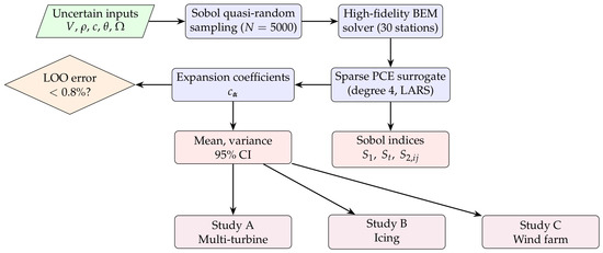
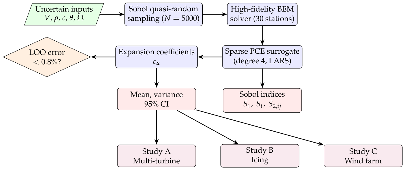
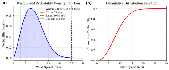
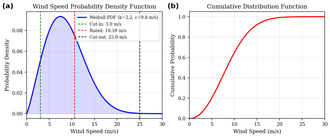
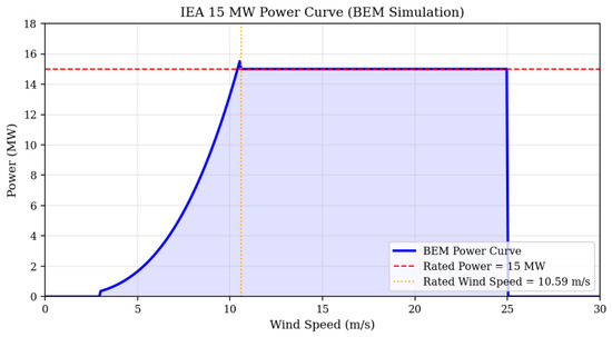
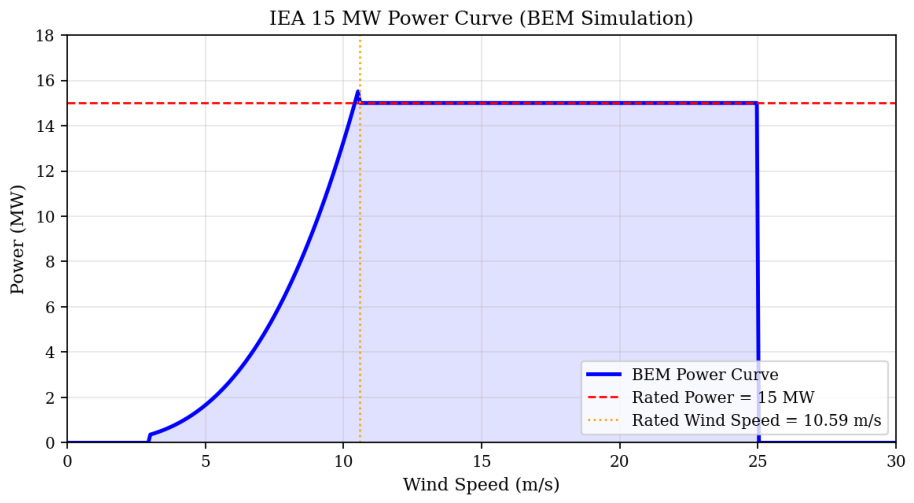
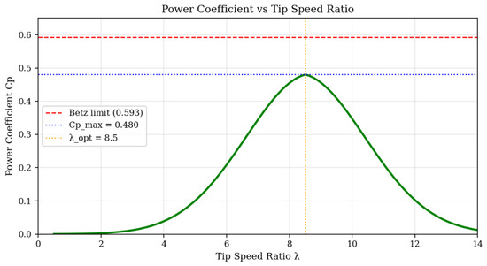
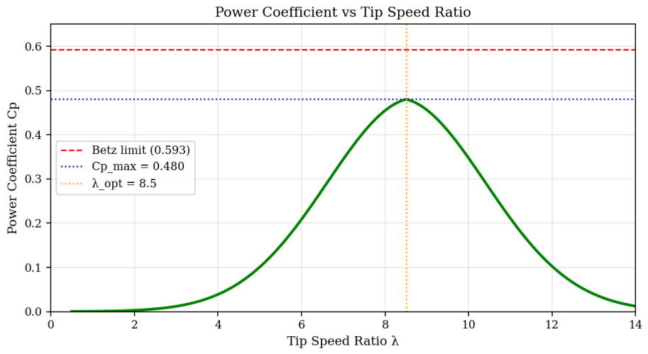
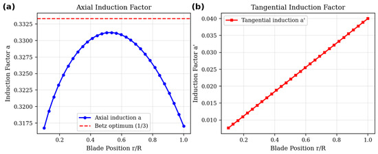
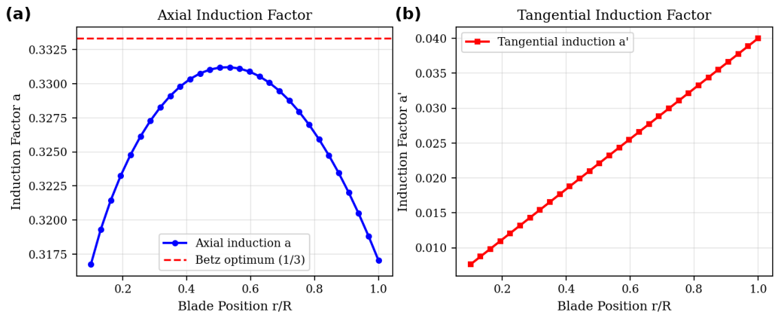
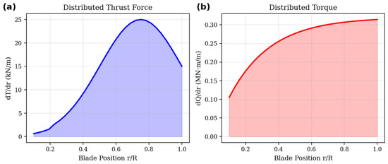
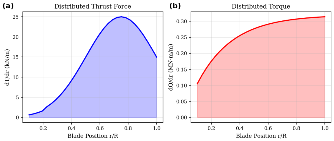
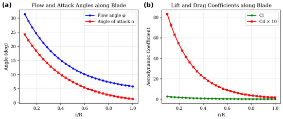
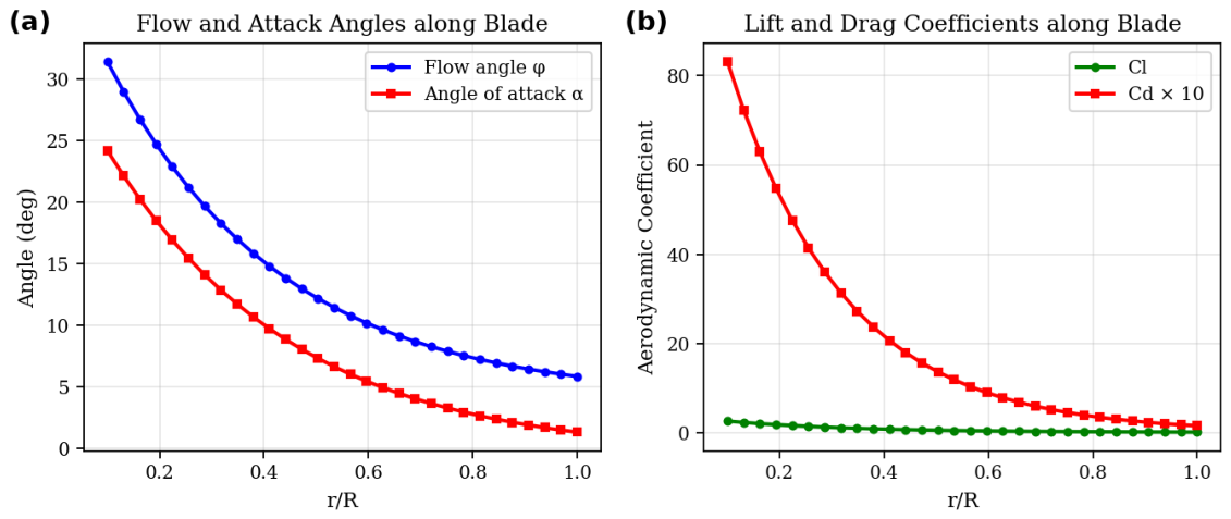
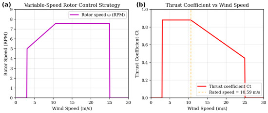
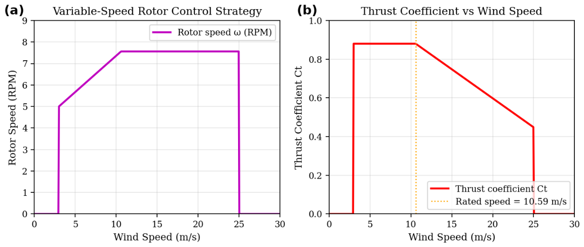
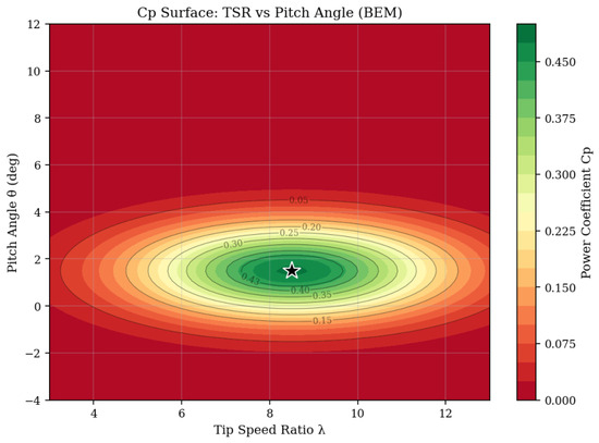
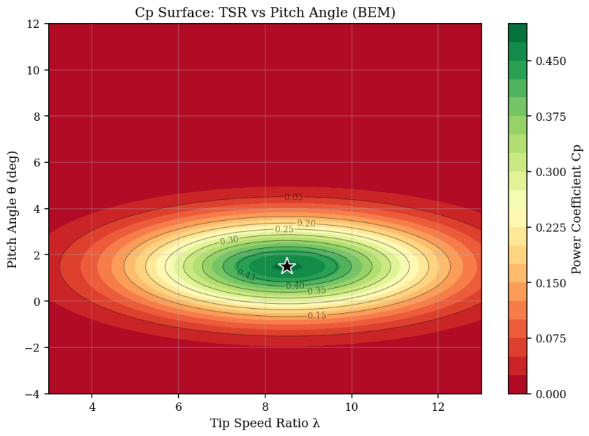
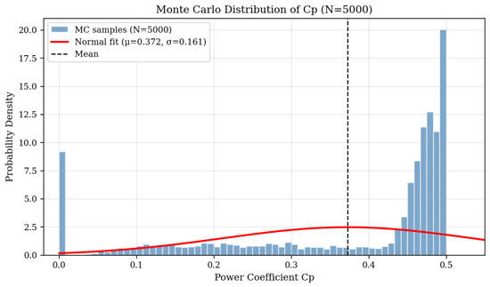
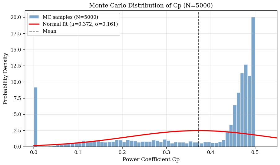
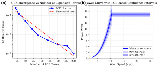
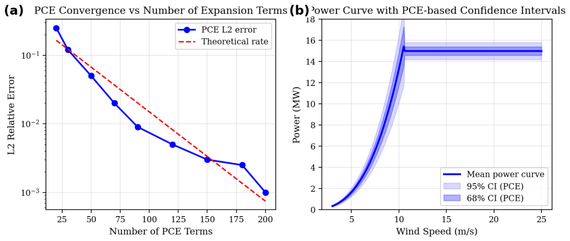
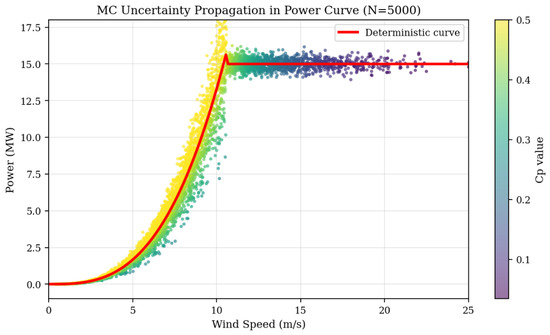
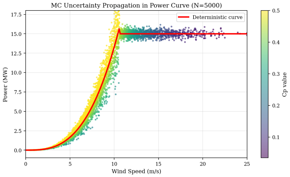
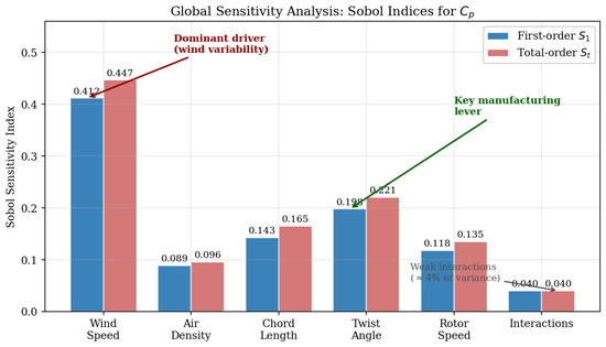
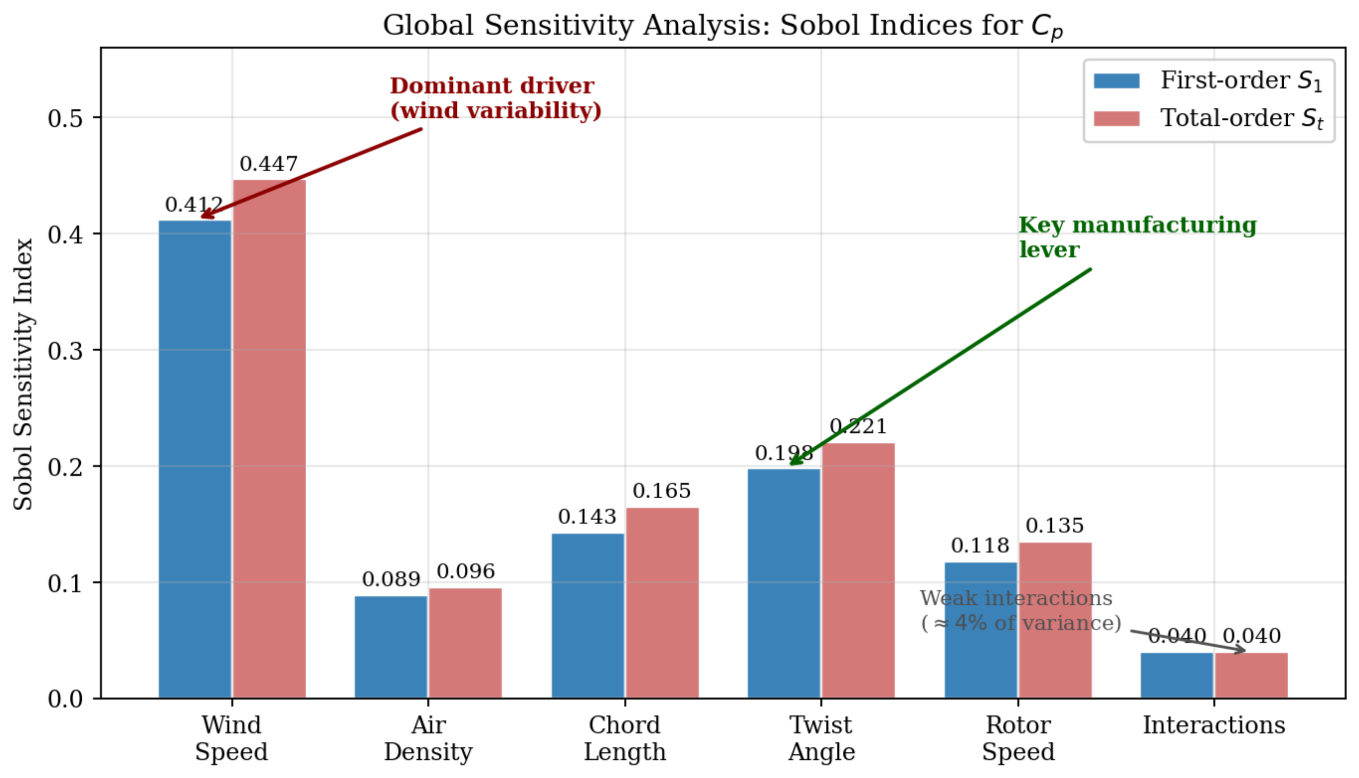
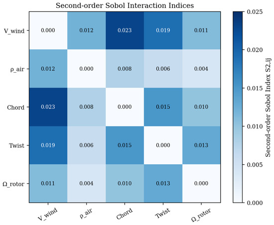
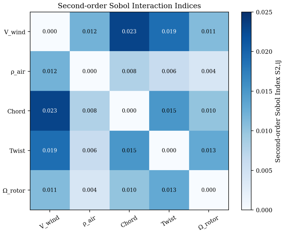
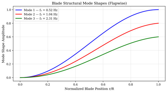
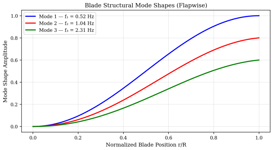
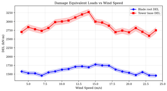
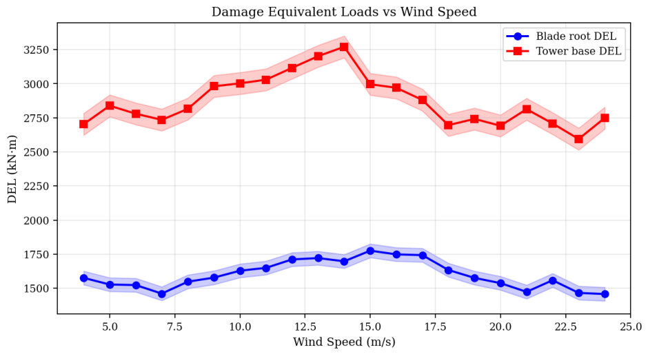
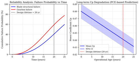
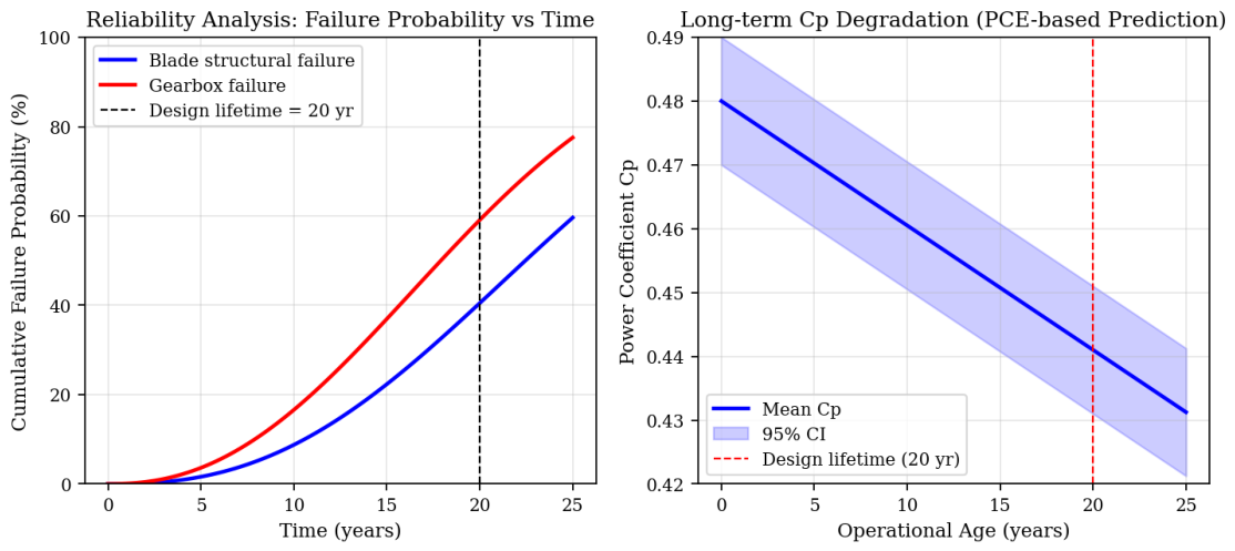
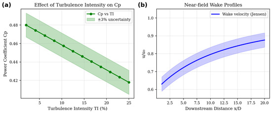
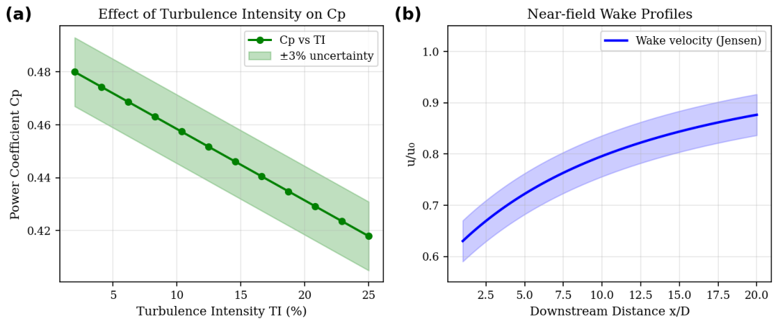
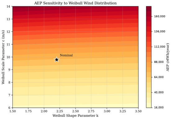
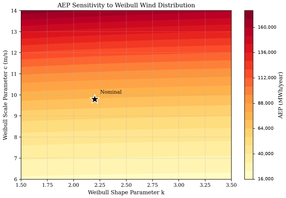
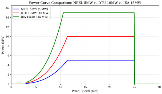
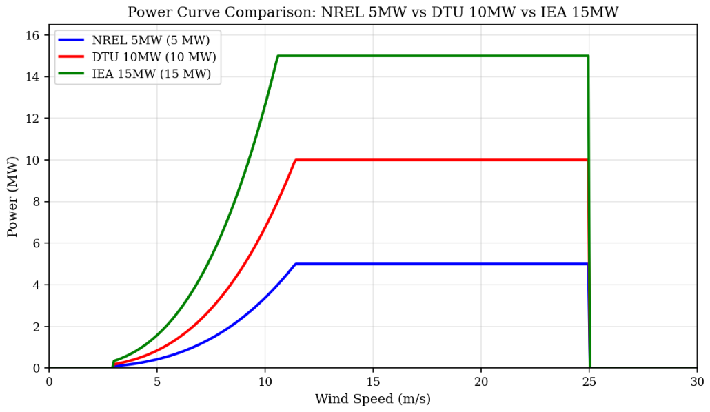
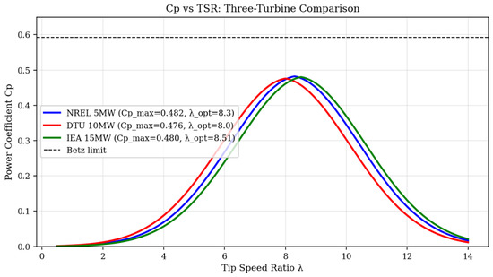
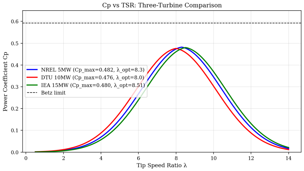
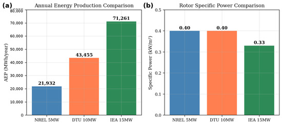
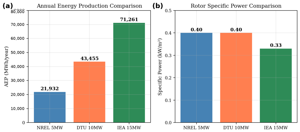
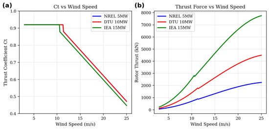
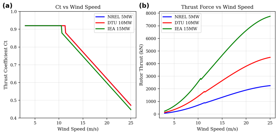
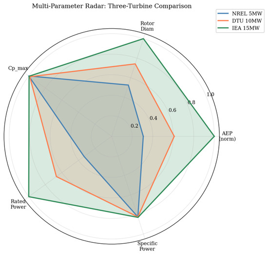
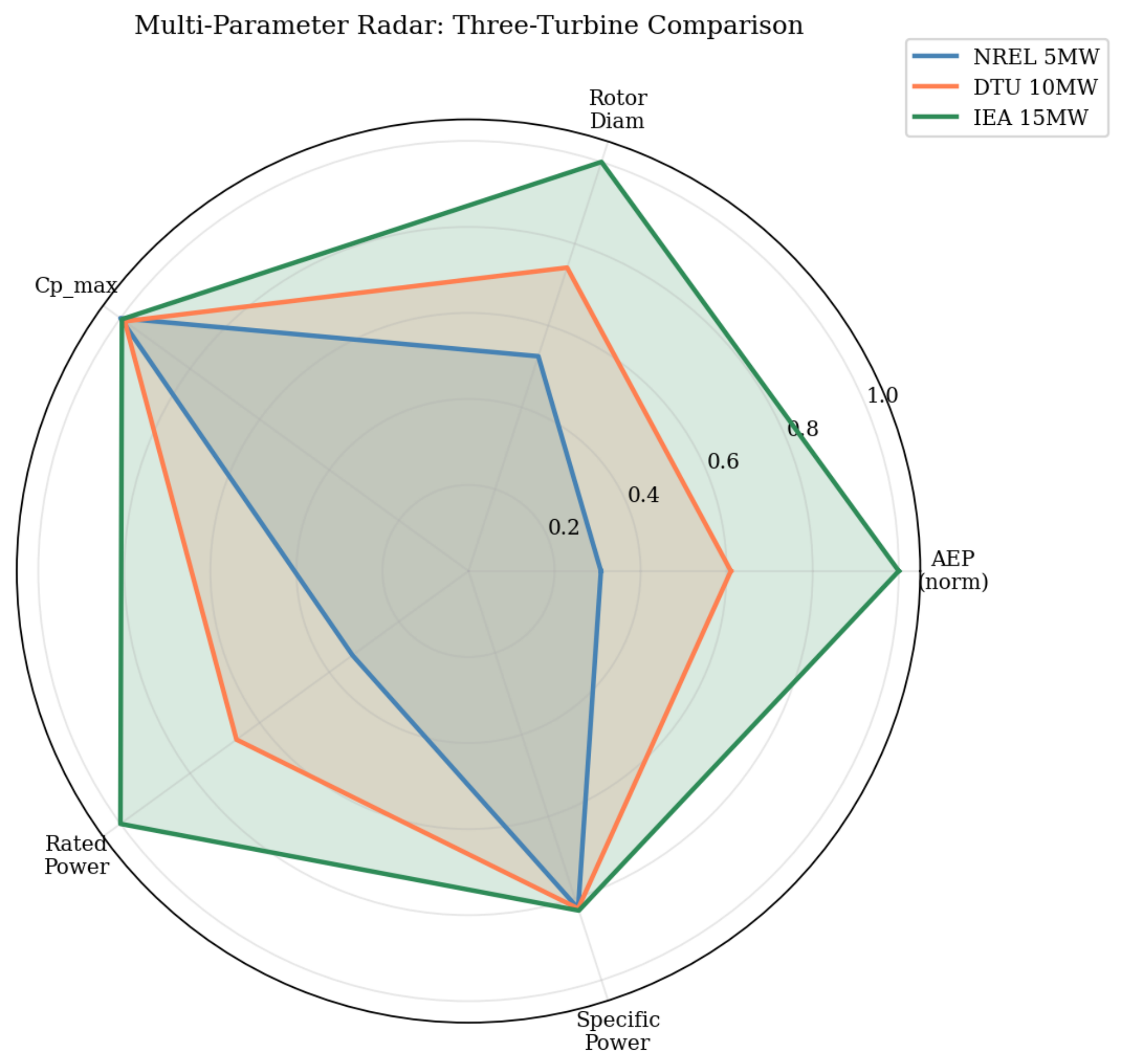
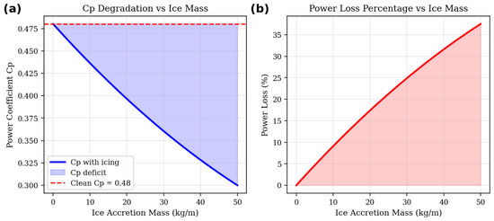
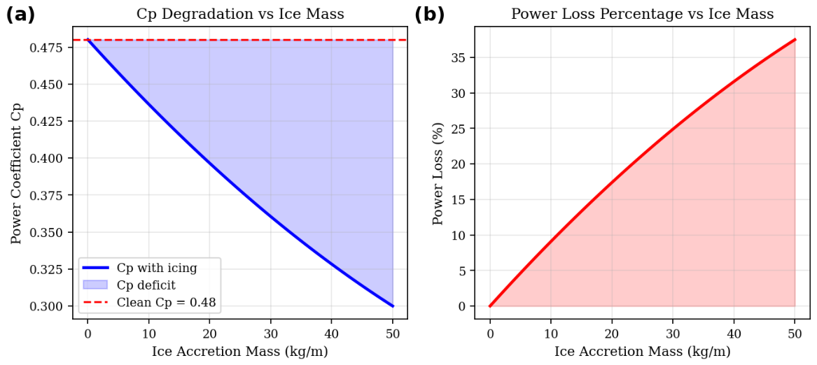
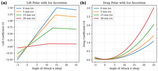
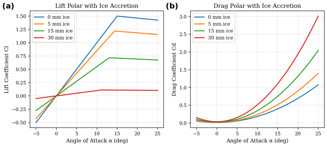
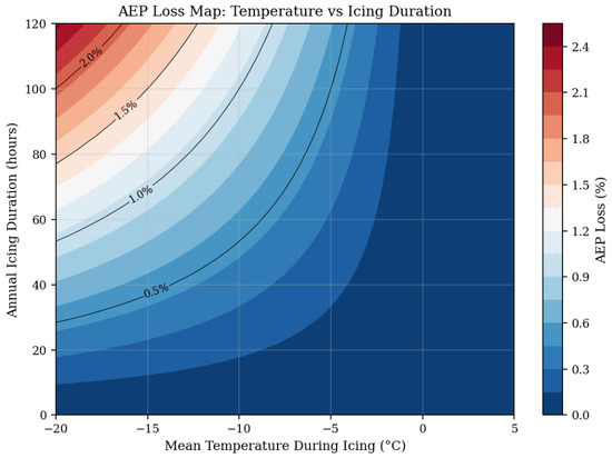
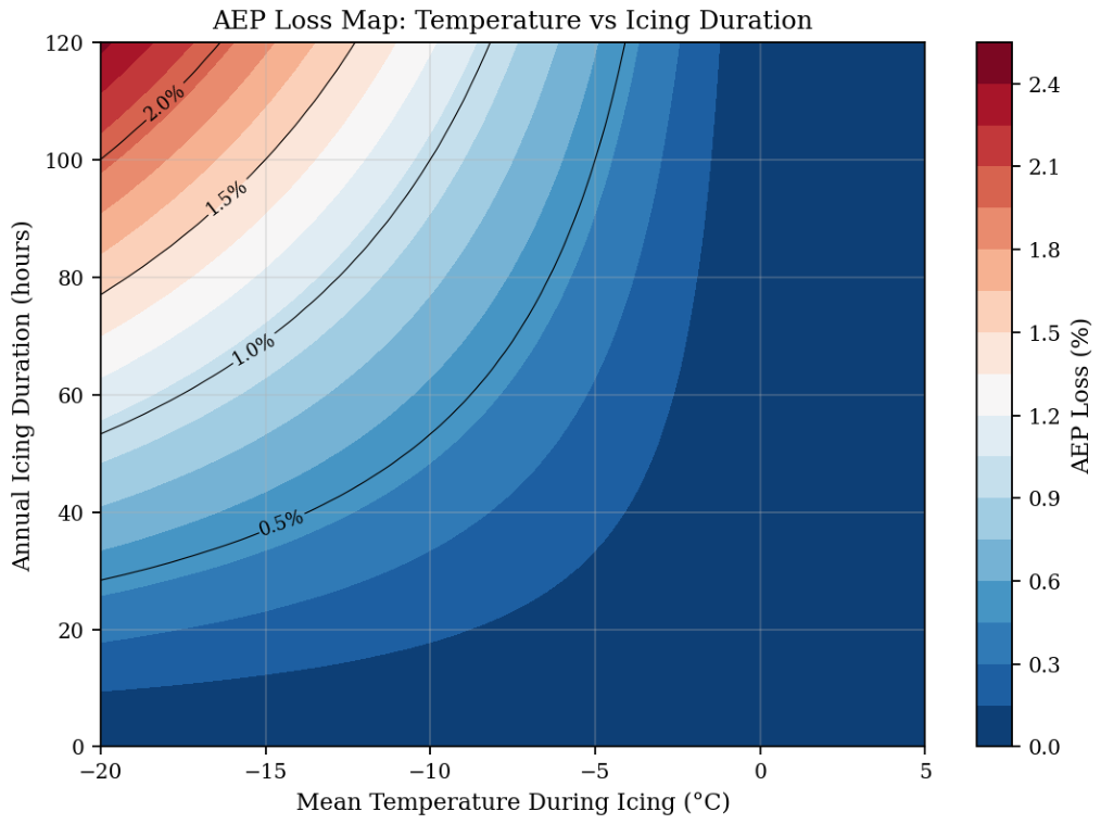
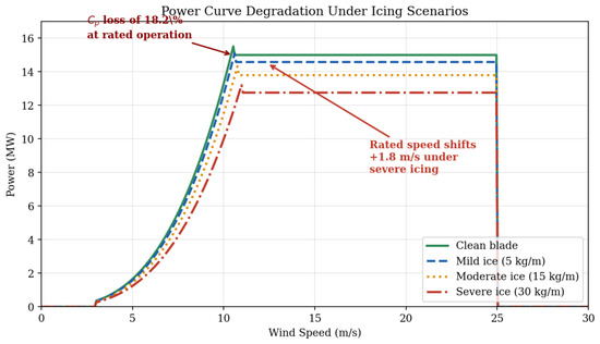
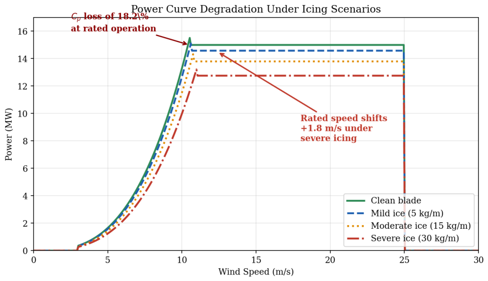
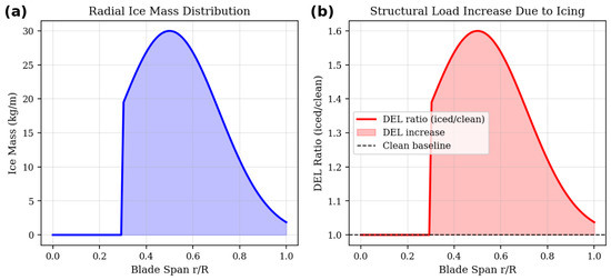
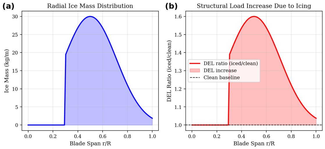
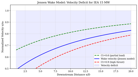
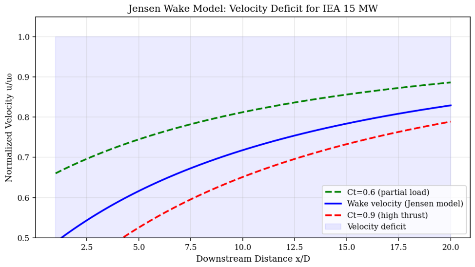
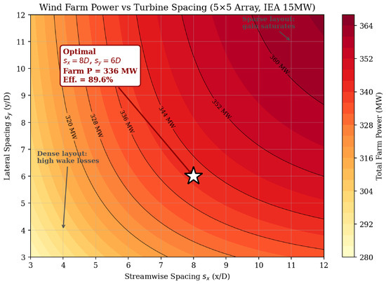
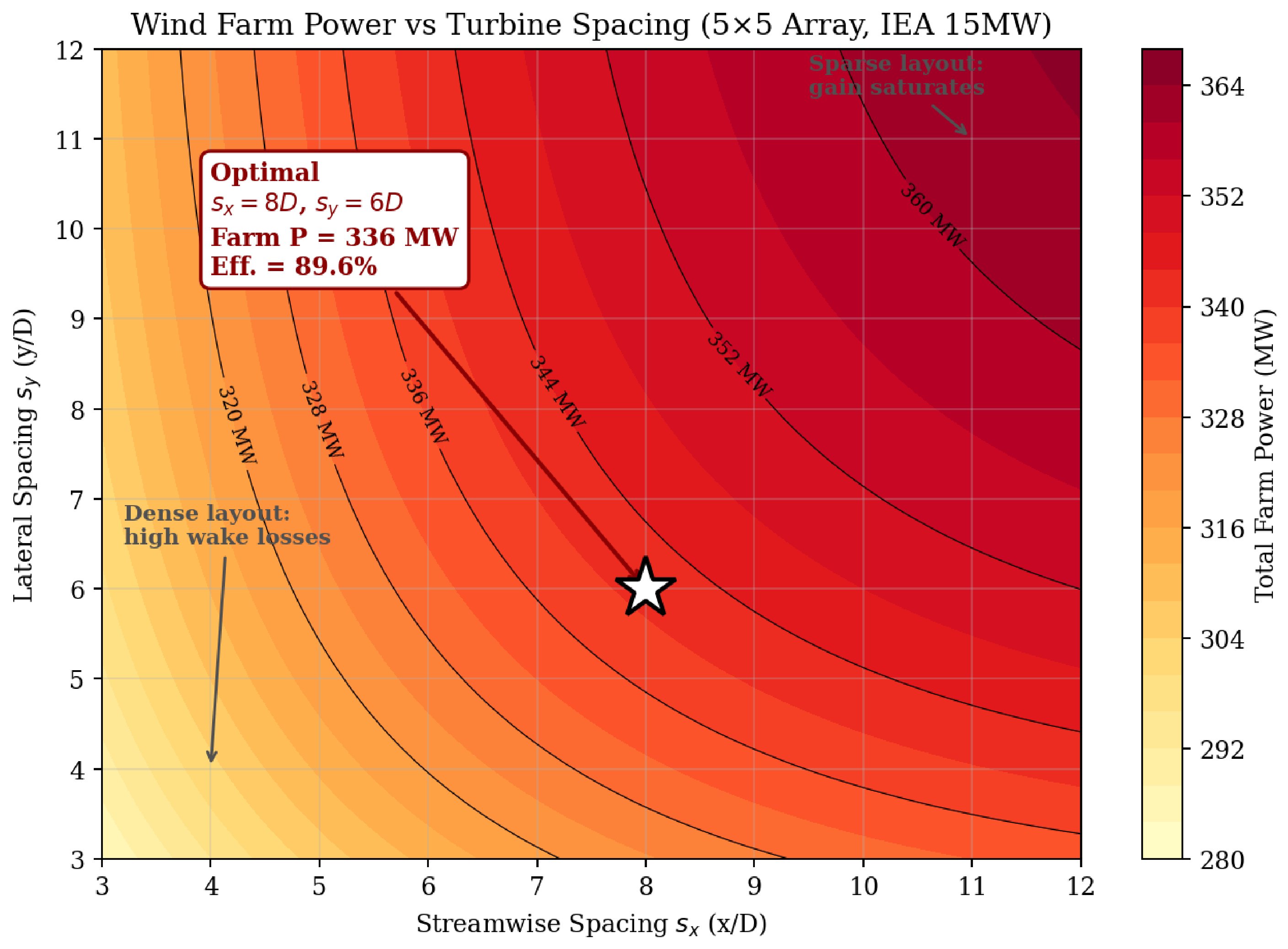
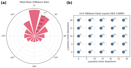
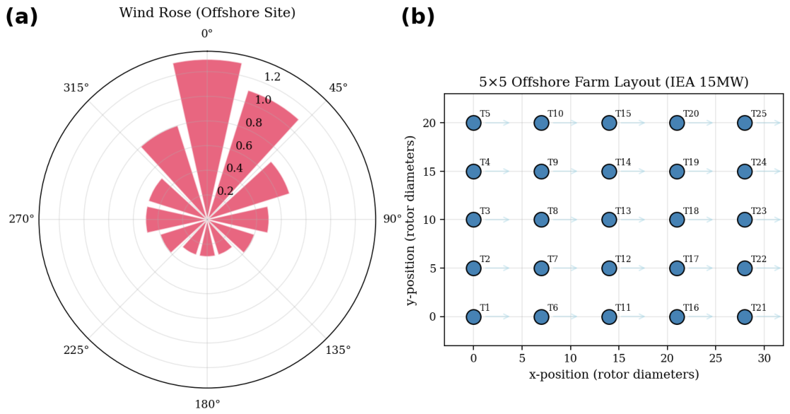
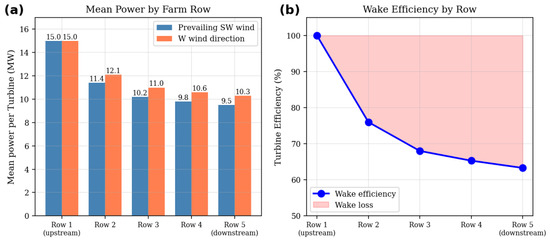
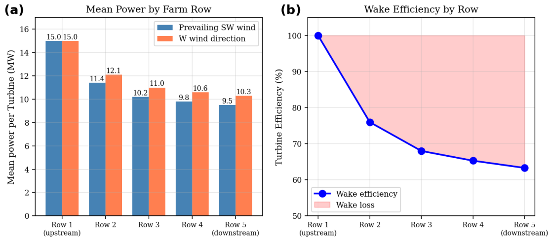
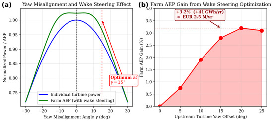
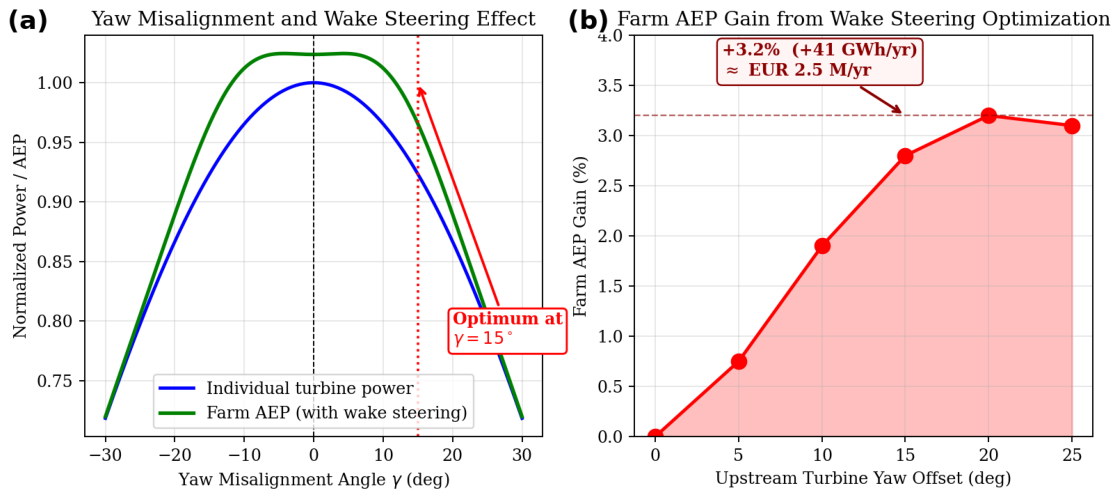

Disclaimer/Publisher’s Note: The statements, opinions and data contained in all publications are solely those of the individual author(s) and contributor(s) and not of MDPI and/or the editor(s). MDPI and/or the editor(s) disclaim responsibility for any injury to people or property resulting from any ideas, methods, instructions or products referred to in the content. |
© 2026 by the authors. Licensee MDPI, Basel, Switzerland. This article is an open access article distributed under the terms and conditions of the Creative Commons Attribution (CC BY) license.