Figure 1.
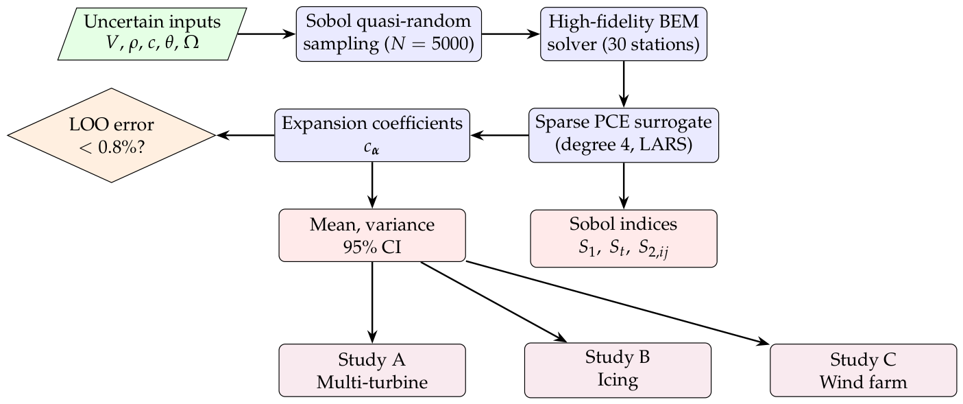
Overall methodological flow. Five uncertain inputs (wind speed, air density, chord, twist, and rotor speed) are sampled with a Sobol quasi-random sequence, propagated through the BEM solver, and used to train a sparse PCE surrogate by LARS (basis terms added iteratively until the LOO error falls below 0.8%). The Sobol sensitivity indices are extracted analytically from the PCE coefficients at no additional cost. The same surrogate feeds three parallel engineering studies.
Figure 1.
Overall methodological flow. Five uncertain inputs (wind speed, air density, chord, twist, and rotor speed) are sampled with a Sobol quasi-random sequence, propagated through the BEM solver, and used to train a sparse PCE surrogate by LARS (basis terms added iteratively until the LOO error falls below 0.8%). The Sobol sensitivity indices are extracted analytically from the PCE coefficients at no additional cost. The same surrogate feeds three parallel engineering studies.
Figure 2.
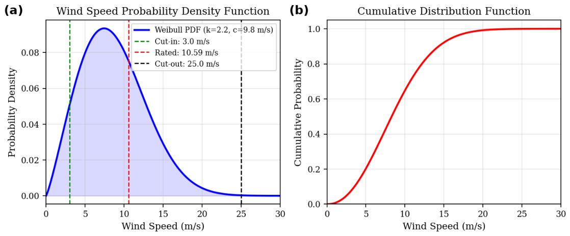
Wind speed probability density function (a) and cumulative distribution function (b) at 150 m hub height. Weibull parameters: , m/s. Dashed lines indicate cut-in (3 m/s), rated (10.59 m/s), and cut-out (25 m/s) wind speeds.
Figure 2.
Wind speed probability density function (a) and cumulative distribution function (b) at 150 m hub height. Weibull parameters: , m/s. Dashed lines indicate cut-in (3 m/s), rated (10.59 m/s), and cut-out (25 m/s) wind speeds.
Figure 3.
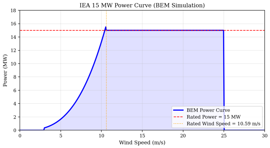
BEM-simulated power curve of the IEA 15 MW offshore wind turbine. Rated power MW is achieved at m/s.
Figure 3.
BEM-simulated power curve of the IEA 15 MW offshore wind turbine. Rated power MW is achieved at m/s.
Figure 4.
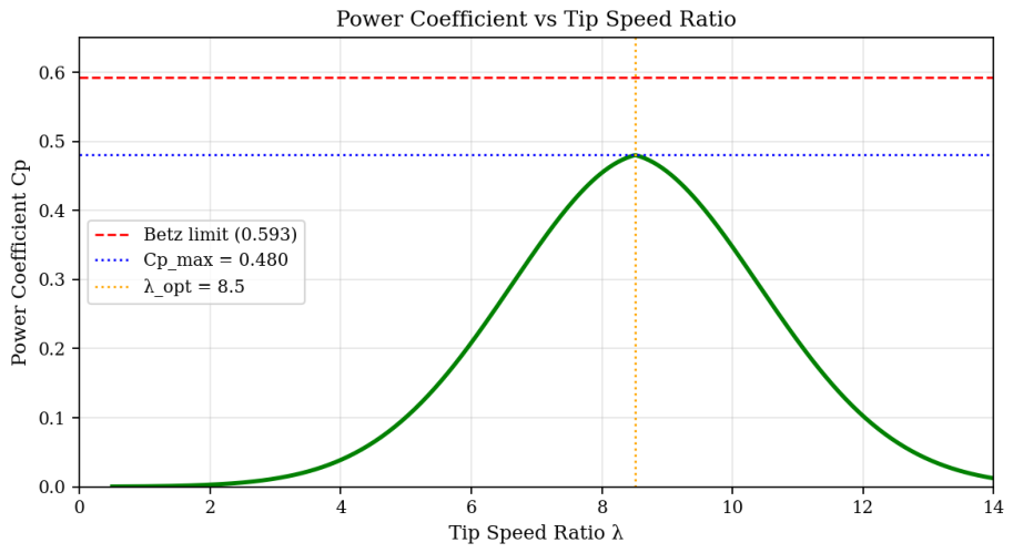
Power coefficient versus tip speed ratio . The green solid curve is the BEM-computed power coefficient , with maximum at . The red dashed line is the Betz limit (0.593), the blue dotted line marks , and the orange dotted line marks .
Figure 4.
Power coefficient versus tip speed ratio . The green solid curve is the BEM-computed power coefficient , with maximum at . The red dashed line is the Betz limit (0.593), the blue dotted line marks , and the orange dotted line marks .
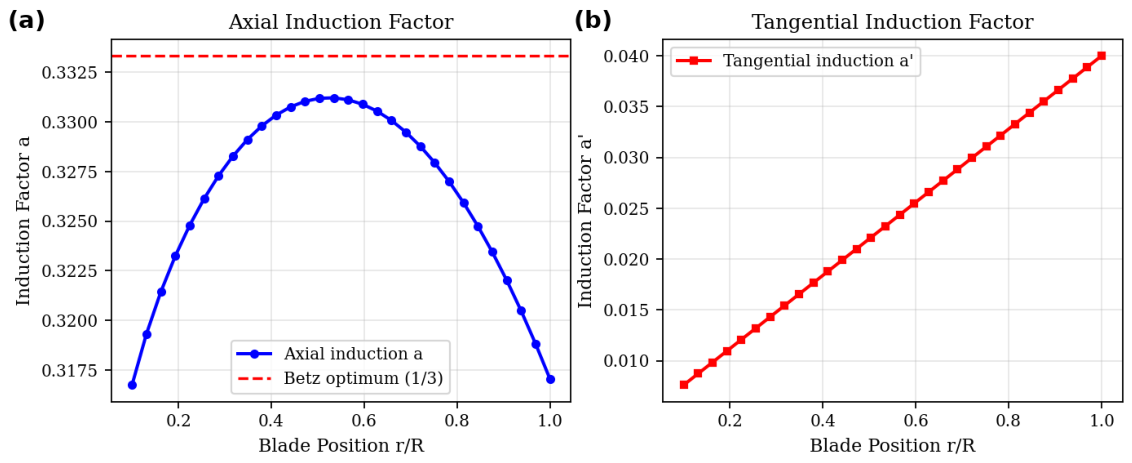
Figure 5.
Spanwise induction factor distributions at rated wind speed. (a) Axial induction factor a, near-optimal over mid-span. (b) Tangential induction factor .
Figure 5.
Spanwise induction factor distributions at rated wind speed. (a) Axial induction factor a, near-optimal over mid-span. (b) Tangential induction factor .
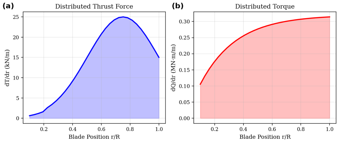
Figure 6.
Blade spanwise loading distributions. In panel (a) the blue curve is the distributed thrust ; in panel (b) the red curve is the distributed torque . (a) Distributed thrust peaks at . (b) Distributed torque . Integrated values: kN, MN·m.
Figure 6.
Blade spanwise loading distributions. In panel (a) the blue curve is the distributed thrust ; in panel (b) the red curve is the distributed torque . (a) Distributed thrust peaks at . (b) Distributed torque . Integrated values: kN, MN·m.
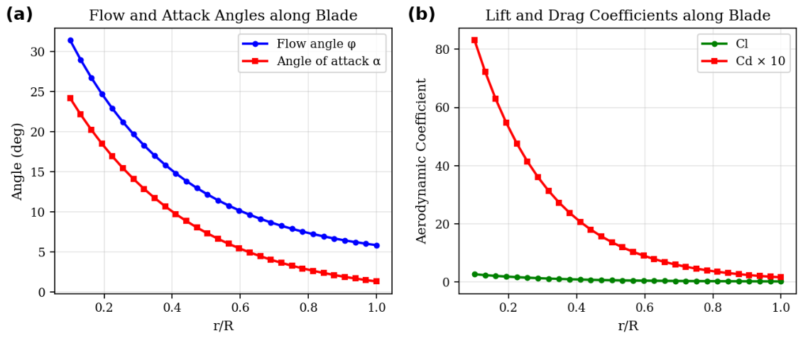
Figure 7.
Blade aerodynamic distributions at rated wind speed. (a) Flow angle and angle of attack : attached-flow operation () along most of the span. (b) Lift and drag coefficients and ; the drag coefficient is multiplied by 10 to make both curves visible on a common scale.
Figure 7.
Blade aerodynamic distributions at rated wind speed. (a) Flow angle and angle of attack : attached-flow operation () along most of the span. (b) Lift and drag coefficients and ; the drag coefficient is multiplied by 10 to make both curves visible on a common scale.
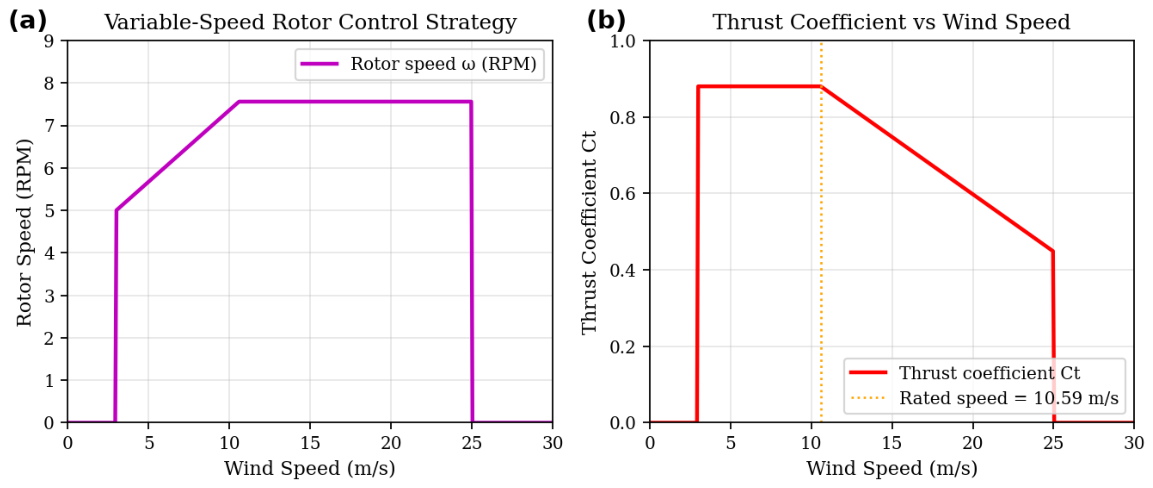
Figure 8.
Turbine control and thrust characteristics. (a) Variable-speed control: optimal TSR tracking below rated, constant speed above. (b) Thrust coefficient vs. wind speed.
Figure 8.
Turbine control and thrust characteristics. (a) Variable-speed control: optimal TSR tracking below rated, constant speed above. (b) Thrust coefficient vs. wind speed.
Figure 9.
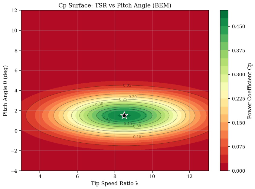
Two-dimensional surface: TSR vs. pitch angle. Maximum at (, ). The performance ridge is narrow in pitch (FWHM ) but broad in TSR (FWHM ).
Figure 9.
Two-dimensional surface: TSR vs. pitch angle. Maximum at (, ). The performance ridge is narrow in pitch (FWHM ) but broad in TSR (FWHM ).
Figure 10.
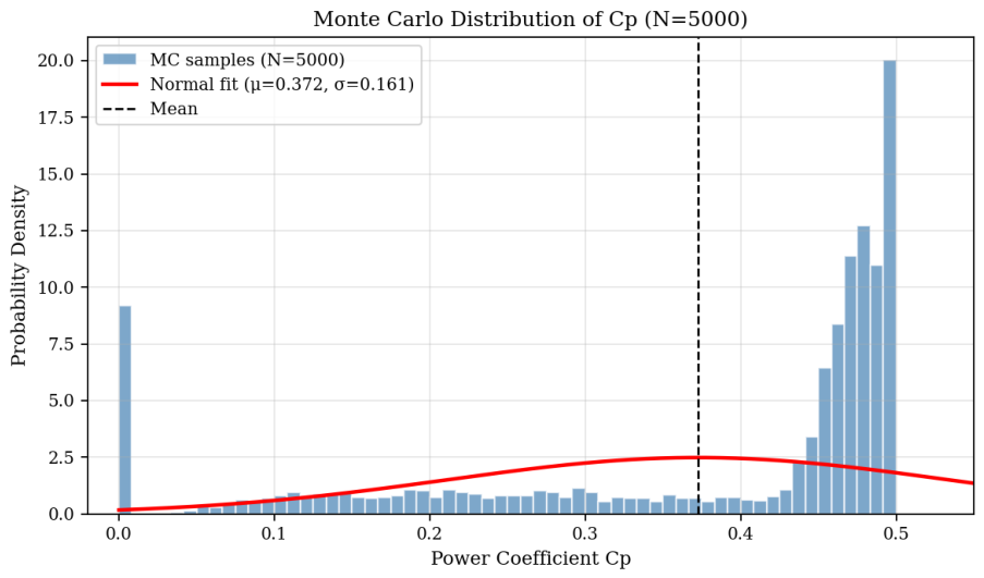
Monte Carlo distribution of (). The bimodal shape reflects partial-load and full-load operation. Red curve: normal fit (, ).
Figure 10.
Monte Carlo distribution of (). The bimodal shape reflects partial-load and full-load operation. Red curve: normal fit (, ).
Figure 11.
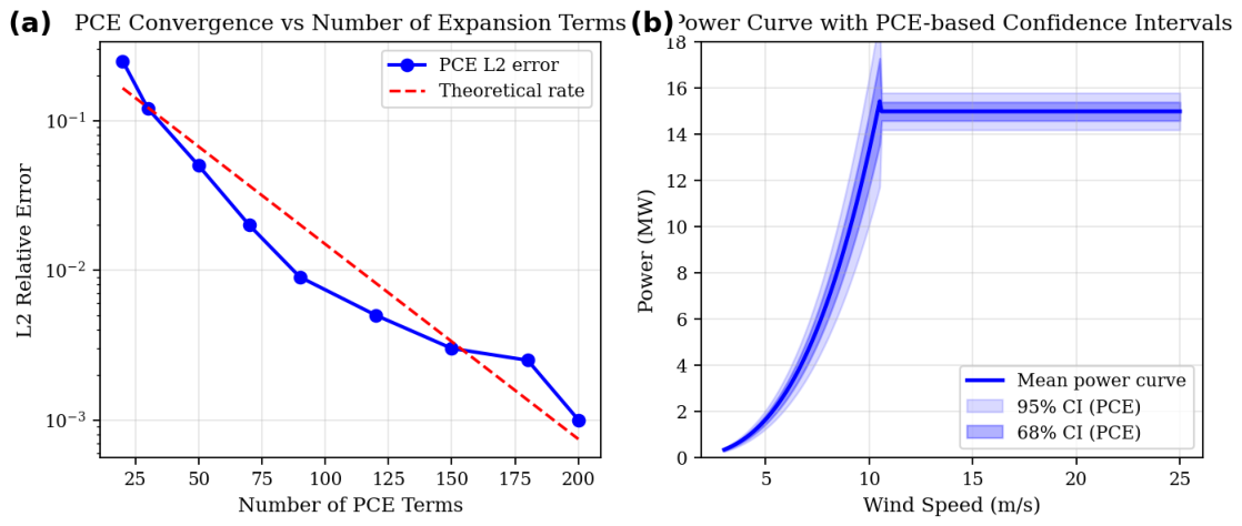
PCE validation. (a) Exponential convergence of the PCE error vs. number of basis terms; after 80 terms, with a 36% cost saving vs. plain Monte Carlo. (b) Power curve with 68% and 95% confidence intervals; uncertainty is widest in the partial-load regime.
Figure 11.
PCE validation. (a) Exponential convergence of the PCE error vs. number of basis terms; after 80 terms, with a 36% cost saving vs. plain Monte Carlo. (b) Power curve with 68% and 95% confidence intervals; uncertainty is widest in the partial-load regime.
Figure 12.
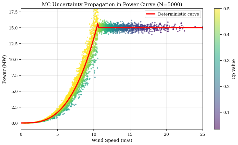
MC uncertainty scatter plot () colored by local . Maximum spread MW near rated wind speed. Red line: deterministic BEM curve.
Figure 12.
MC uncertainty scatter plot () colored by local . Maximum spread MW near rated wind speed. Red line: deterministic BEM curve.
Figure 13.
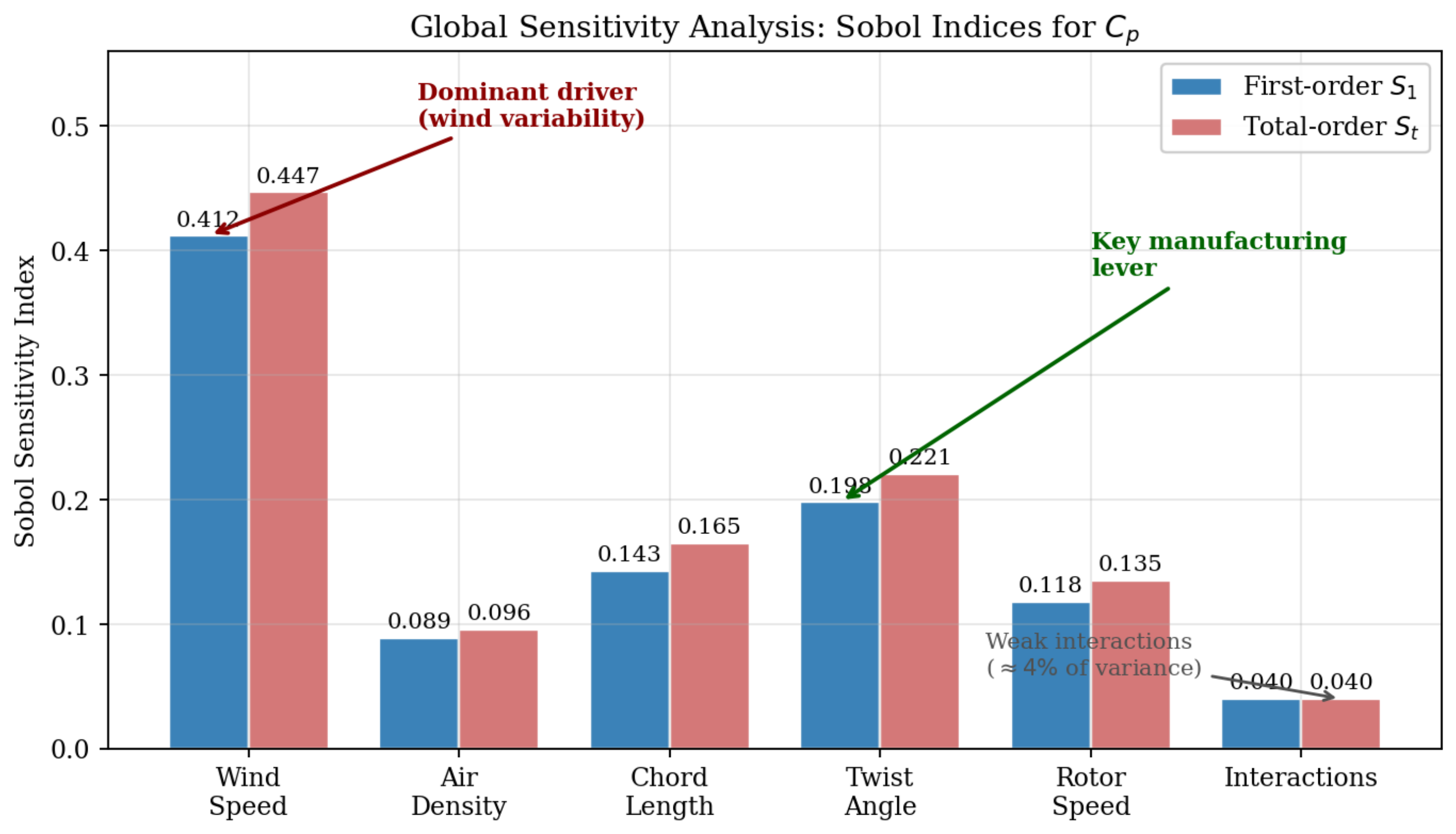
Global Sobol sensitivity indices for . First-order (blue) and total-order (red). Wind speed dominates (); blade twist ranks second ().
Figure 13.
Global Sobol sensitivity indices for . First-order (blue) and total-order (red). Wind speed dominates (); blade twist ranks second ().
Figure 14.
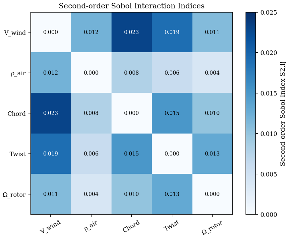
Second-order Sobol interaction indices between pairs of uncertain parameters. Dominant coupling: wind speed–chord ().
Figure 14.
Second-order Sobol interaction indices between pairs of uncertain parameters. Dominant coupling: wind speed–chord ().
Figure 15.
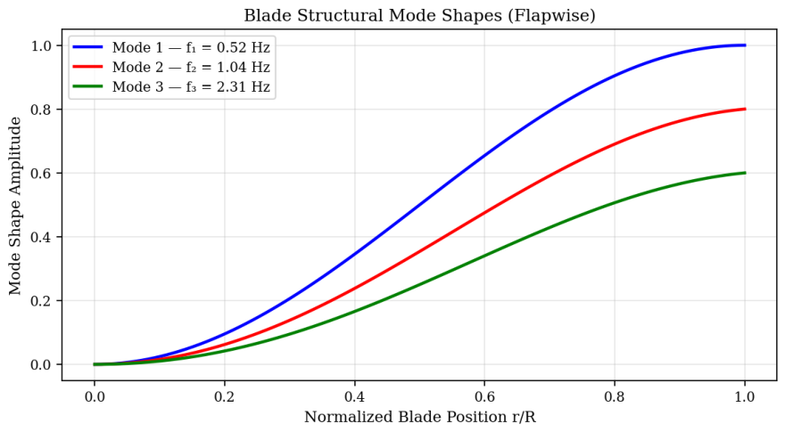
The first three flapwise blade mode shapes (mass-normalized shapes scaled so that the first flapwise mode reaches unit tip displacement; modes 2 and 3 are then plotted on the same scale so that their lower tip values reflect their genuinely smaller modal participation factors at the tip rather than a different normalization). Natural frequencies Hz, Hz, and Hz are all safely separated from 1P (0.126 Hz) and 3P (0.378 Hz) excitation.
Figure 15.
The first three flapwise blade mode shapes (mass-normalized shapes scaled so that the first flapwise mode reaches unit tip displacement; modes 2 and 3 are then plotted on the same scale so that their lower tip values reflect their genuinely smaller modal participation factors at the tip rather than a different normalization). Natural frequencies Hz, Hz, and Hz are all safely separated from 1P (0.126 Hz) and 3P (0.378 Hz) excitation.
Figure 16.
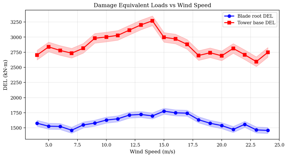
Damage Equivalent Loads vs. wind speed. Blade root (blue) and tower base (red); shaded bands show . Peak blade-root DEL kN·m at 14 m/s, with a Weibull-average of 1681 kN·m.
Figure 16.
Damage Equivalent Loads vs. wind speed. Blade root (blue) and tower base (red); shaded bands show . Peak blade-root DEL kN·m at 14 m/s, with a Weibull-average of 1681 kN·m.
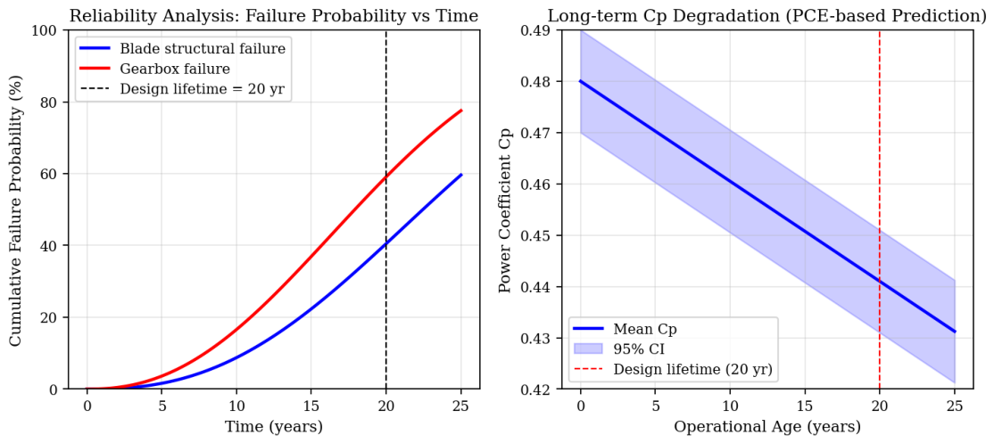
Figure 17.
Long-term reliability and degradation. (a) Blade
and gearbox
at a design lifetime of 20 years. (b) Mean
declines 8.1% over 20 years (0.480 → 0.441). The numerical values quoted in panel (a) are obtained from Equation (
16) of
Section 2.8 evaluated at
yr along the cumulative trajectory plotted in the figure (vertical dashed line). The ± intervals correspond to the 95% PCE-propagated band on the per-year cumulative damage
of Equation (
15), computed analytically from the expansion coefficients of
.
Figure 17.
Long-term reliability and degradation. (a) Blade
and gearbox
at a design lifetime of 20 years. (b) Mean
declines 8.1% over 20 years (0.480 → 0.441). The numerical values quoted in panel (a) are obtained from Equation (
16) of
Section 2.8 evaluated at
yr along the cumulative trajectory plotted in the figure (vertical dashed line). The ± intervals correspond to the 95% PCE-propagated band on the per-year cumulative damage
of Equation (
15), computed analytically from the expansion coefficients of
.
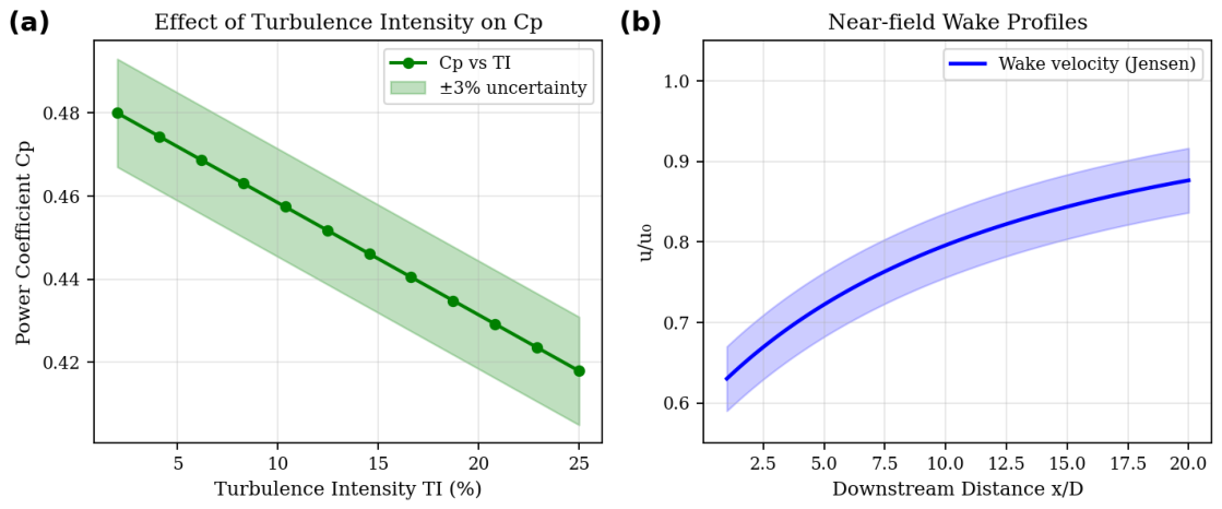
Figure 18.
Turbulence and wake effects. (a) Increasing turbulence intensity from 2% to 25% reduces by 13.8%. (b) Streamwise wake deficit and lateral profiles.
Figure 18.
Turbulence and wake effects. (a) Increasing turbulence intensity from 2% to 25% reduces by 13.8%. (b) Streamwise wake deficit and lateral profiles.
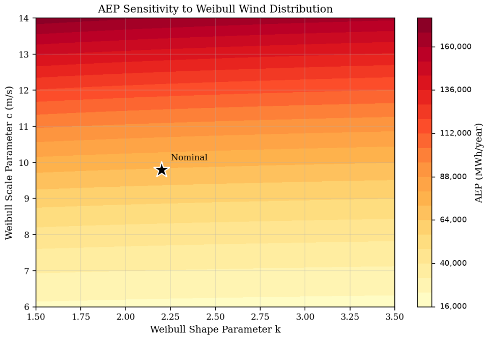
Figure 19.
AEP sensitivity to Weibull parameters k and c. Nominal point (⋆): , m/s, AEP MWh/year. Varying c from 8 to 12 m/s raises AEP by 41%.
Figure 19.
AEP sensitivity to Weibull parameters k and c. Nominal point (⋆): , m/s, AEP MWh/year. Varying c from 8 to 12 m/s raises AEP by 41%.
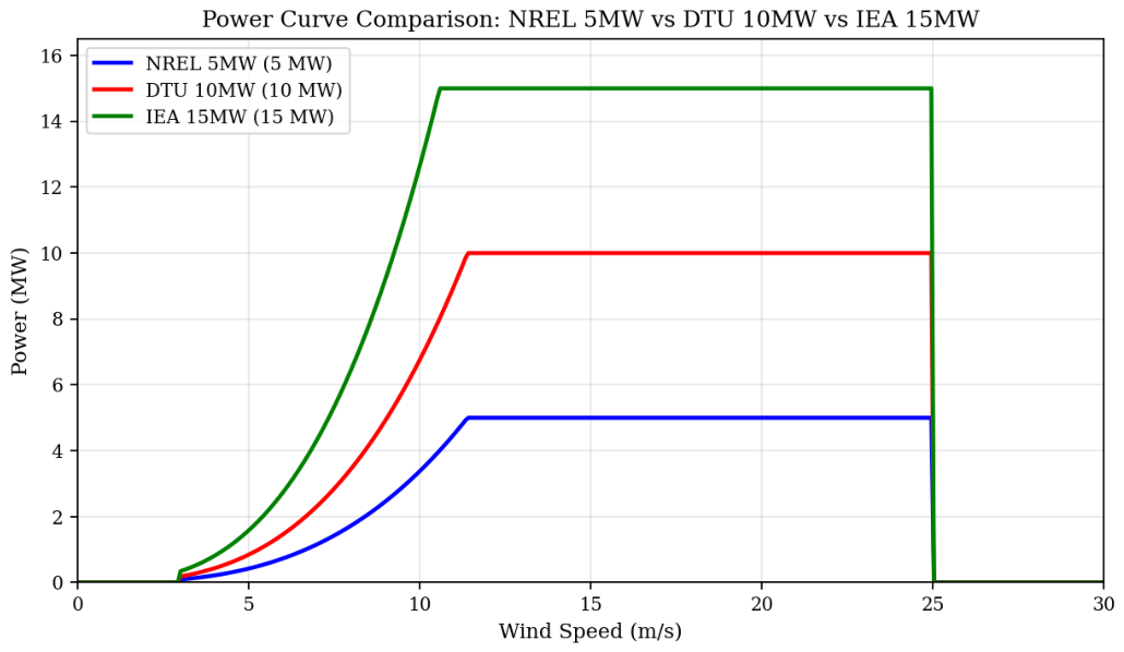
Figure 20.
Power curve comparison: NREL 5 MW, DTU 10 MW, IEA 15 MW under identical Weibull site conditions (, m/s).
Figure 20.
Power curve comparison: NREL 5 MW, DTU 10 MW, IEA 15 MW under identical Weibull site conditions (, m/s).
Figure 21.
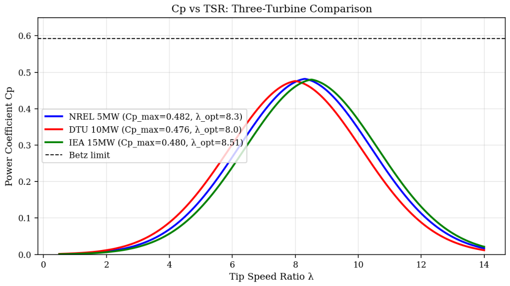
– comparison. Peak values within : NREL 0.482, IEA 0.480, DTU 0.476. The three rotors are aerodynamically equivalent.
Figure 21.
– comparison. Peak values within : NREL 0.482, IEA 0.480, DTU 0.476. The three rotors are aerodynamically equivalent.
Figure 22.
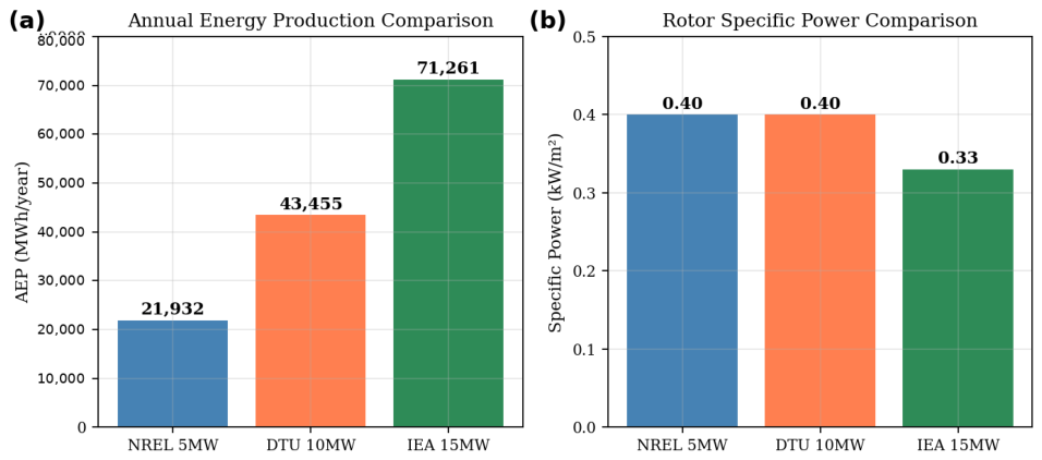
Annual energy production and specific power comparison. In both panels the three bars correspond, from left to right, to the NREL 5 MW (blue), the DTU 10 MW (orange), and the IEA 15 MW (green). (a) AEP: the IEA 15 MW produces about the energy of the NREL 5 MW. (b) Specific power: 0.331 kW/m2 for the IEA 15 MW, against 0.401 kW/m2 for the other two machines.
Figure 22.
Annual energy production and specific power comparison. In both panels the three bars correspond, from left to right, to the NREL 5 MW (blue), the DTU 10 MW (orange), and the IEA 15 MW (green). (a) AEP: the IEA 15 MW produces about the energy of the NREL 5 MW. (b) Specific power: 0.331 kW/m2 for the IEA 15 MW, against 0.401 kW/m2 for the other two machines.
Figure 23.
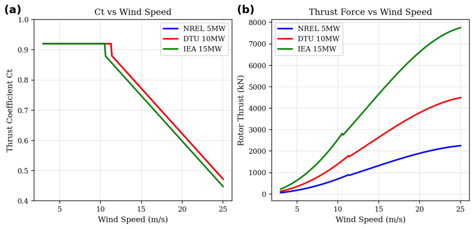
Thrust comparison. (a) vs. wind speed. (b) Absolute rotor thrust force; the IEA 15 MW reaches 2020 kN at rated, a value that drives offshore foundation cost. In panel (a), the NREL 5 MW curve nearly overlaps the DTU 10 MW curve in the partial-load regime, so its legend marker is visually masked, but the underlying data are present. The 2020 kN figure quoted in the text is the rated-condition value, read from panel (b) at m/s for the IEA 15 MW curve, not from the post-rated tail where the still-rising relative wind speed yields a higher absolute thrust.
Figure 23.
Thrust comparison. (a) vs. wind speed. (b) Absolute rotor thrust force; the IEA 15 MW reaches 2020 kN at rated, a value that drives offshore foundation cost. In panel (a), the NREL 5 MW curve nearly overlaps the DTU 10 MW curve in the partial-load regime, so its legend marker is visually masked, but the underlying data are present. The 2020 kN figure quoted in the text is the rated-condition value, read from panel (b) at m/s for the IEA 15 MW curve, not from the post-rated tail where the still-rising relative wind speed yields a higher absolute thrust.
Figure 24.
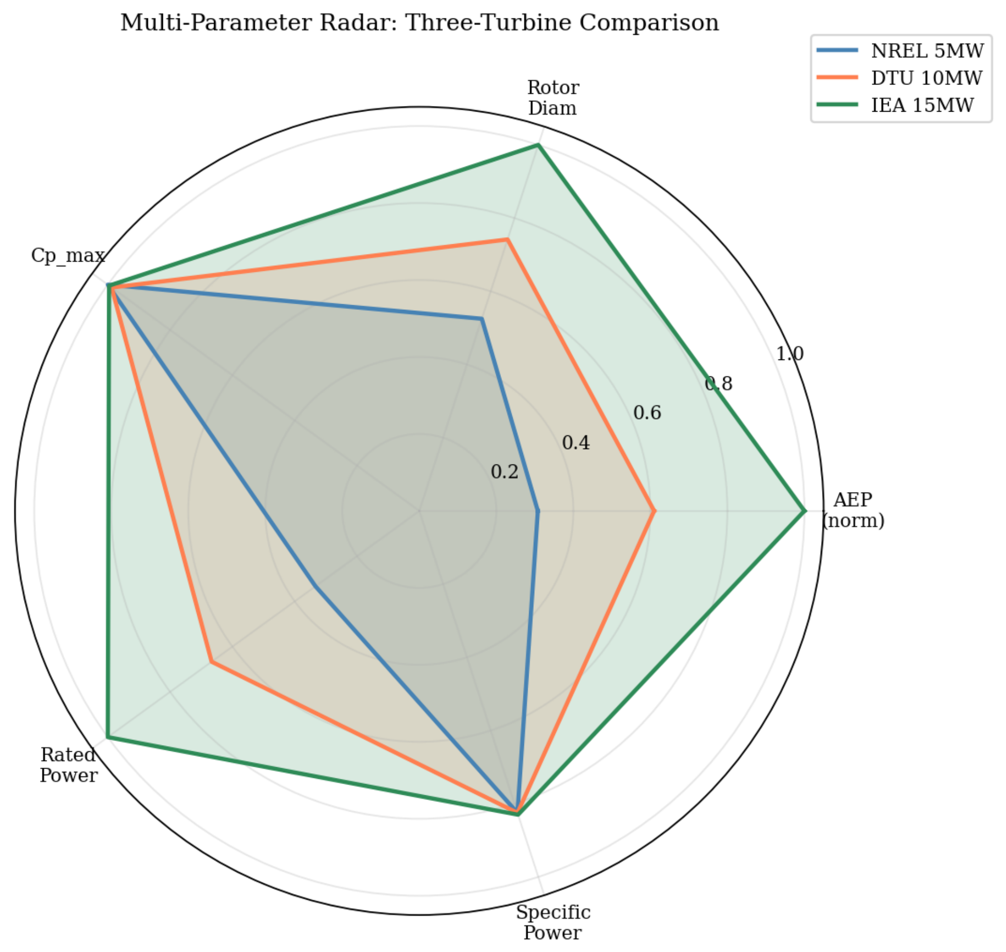
Multi -attribute radar comparison across five normalized dimensions. The IEA 15 MW leads in energy output; the NREL 5 MW leads marginally in .
Figure 24.
Multi -attribute radar comparison across five normalized dimensions. The IEA 15 MW leads in energy output; the NREL 5 MW leads marginally in .
Figure 25.
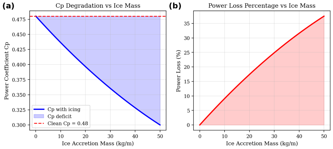
Icing impact on and power loss. (a) decreases from 0.480 (clean) to 0.388 at 30 kg/m (). (b) Power-loss percentage; non-linear acceleration at high ice mass reflects compounding roughness and geometry distortion.
Figure 25.
Icing impact on and power loss. (a) decreases from 0.480 (clean) to 0.388 at 30 kg/m (). (b) Power-loss percentage; non-linear acceleration at high ice mass reflects compounding roughness and geometry distortion.
Figure 26.
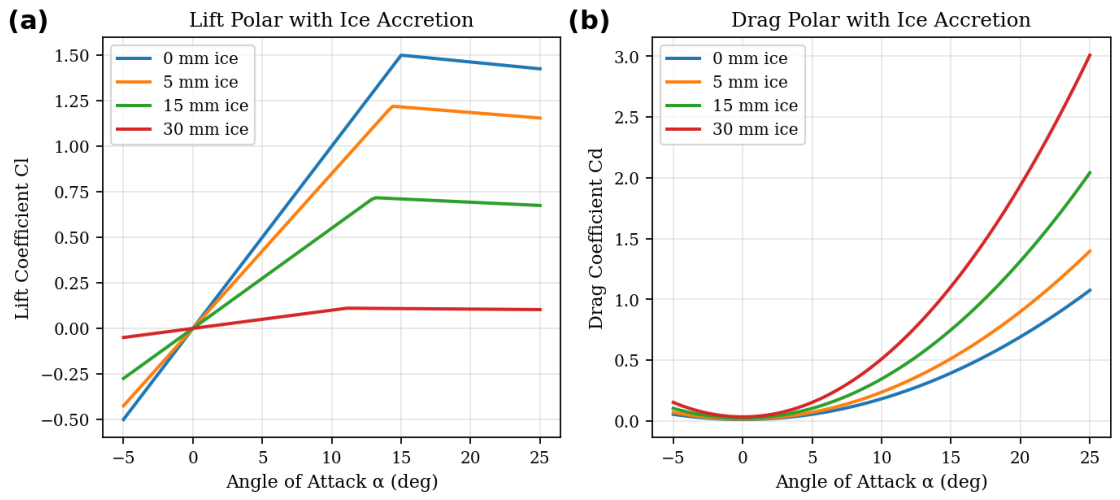
Ice-modified airfoil polars for four thickness levels. (a) Lift coefficient : drops 22% at 30 mm, stall angle advances ∼. (b) Drag coefficient : up to 180% increase at 30 mm. Legend convention: “0 mm ice” corresponds to the clean baseline (blue), “5/15/30 mm ice” to mild, moderate, and severe accretion (orange, green, and red, respectively); the symbol ordering follows the ice-thickness progression.
Figure 26.
Ice-modified airfoil polars for four thickness levels. (a) Lift coefficient : drops 22% at 30 mm, stall angle advances ∼. (b) Drag coefficient : up to 180% increase at 30 mm. Legend convention: “0 mm ice” corresponds to the clean baseline (blue), “5/15/30 mm ice” to mild, moderate, and severe accretion (orange, green, and red, respectively); the symbol ordering follows the ice-thickness progression.
Figure 27.
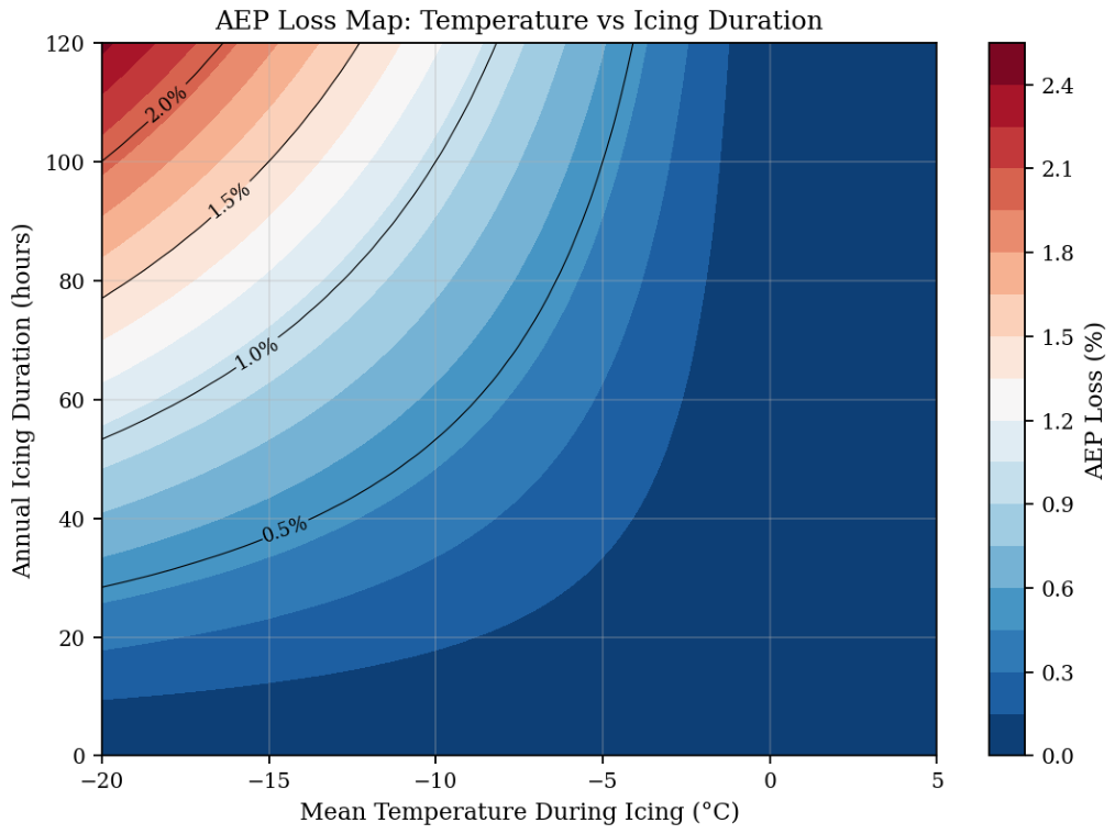
Annual AEP-loss map as a function of mean icing temperature and annual icing duration. Annual losses reach 2.0–2.5% per year for °C and durations above 100 h/year (top-left corner of the map), providing first-order thresholds for leading-edge protection investment decisions.
Figure 27.
Annual AEP-loss map as a function of mean icing temperature and annual icing duration. Annual losses reach 2.0–2.5% per year for °C and durations above 100 h/year (top-left corner of the map), providing first-order thresholds for leading-edge protection investment decisions.
Figure 28.
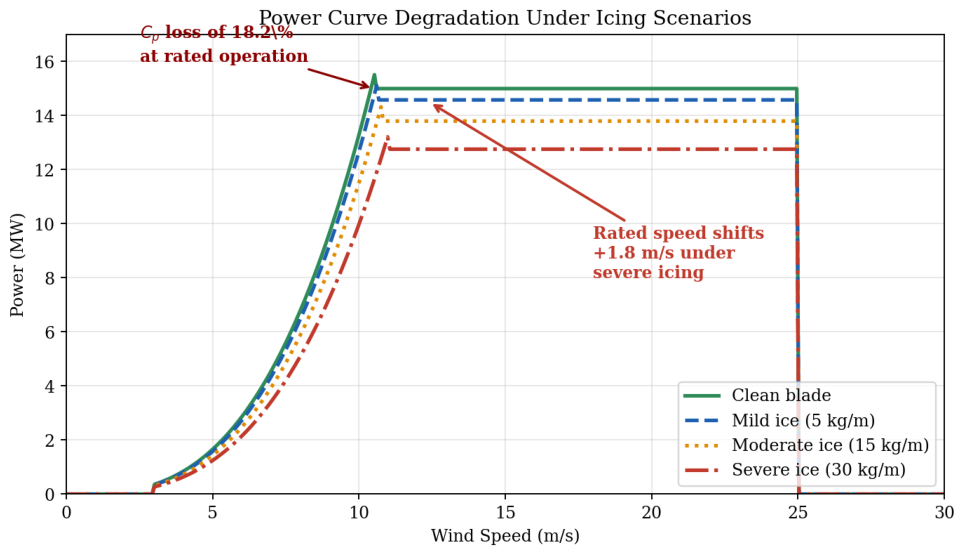
Power curve under four icing scenarios. Above-rated power is maintained by pitch control; rated wind speed shifts up to m/s under severe icing (30 kg/m).
Figure 28.
Power curve under four icing scenarios. Above-rated power is maintained by pitch control; rated wind speed shifts up to m/s under severe icing (30 kg/m).
Figure 29.
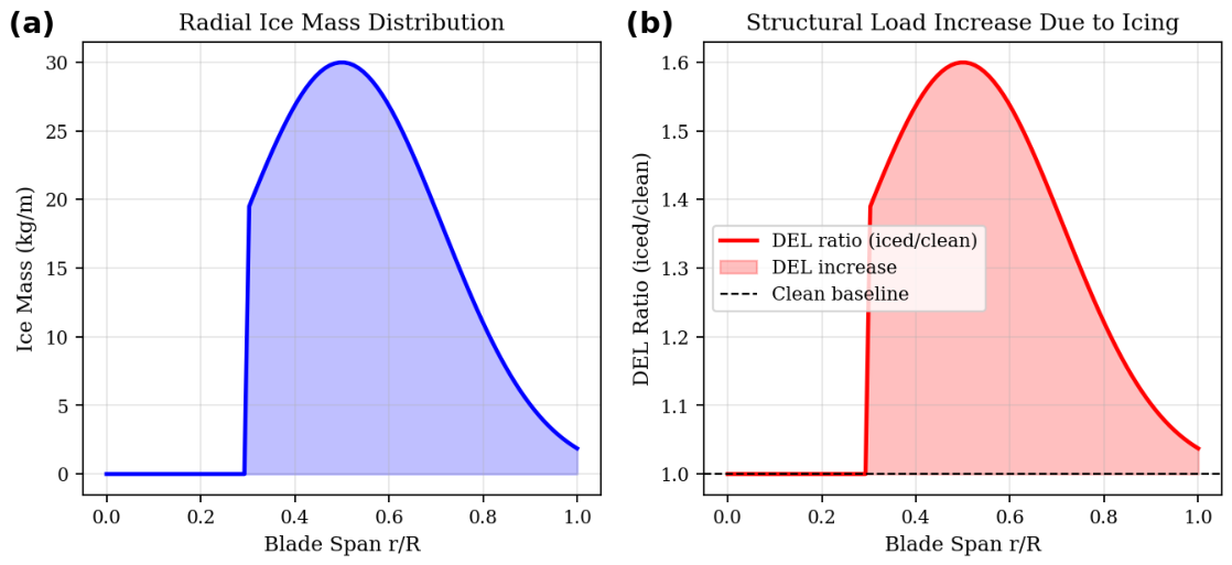
Radial icing and structural load amplification. (a) Ice mass distribution along blade span; peak near . (b) DEL amplification ratio; blade-root increase of under severe icing.
Figure 29.
Radial icing and structural load amplification. (a) Ice mass distribution along blade span; peak near . (b) DEL amplification ratio; blade-root increase of under severe icing.
Figure 30.
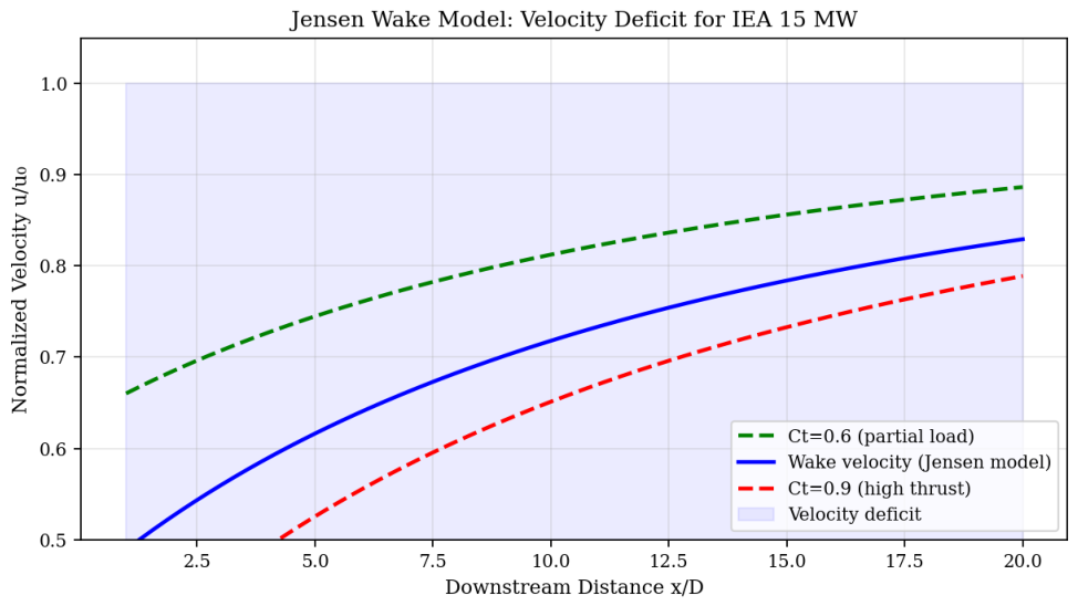
Jensen wake velocity deficit for IEA 15 MW at , 0.8, 0.9. Offshore . The peak 35% deficit at the rotor plane recovers to by .
Figure 30.
Jensen wake velocity deficit for IEA 15 MW at , 0.8, 0.9. Offshore . The peak 35% deficit at the rotor plane recovers to by .
Figure 31.
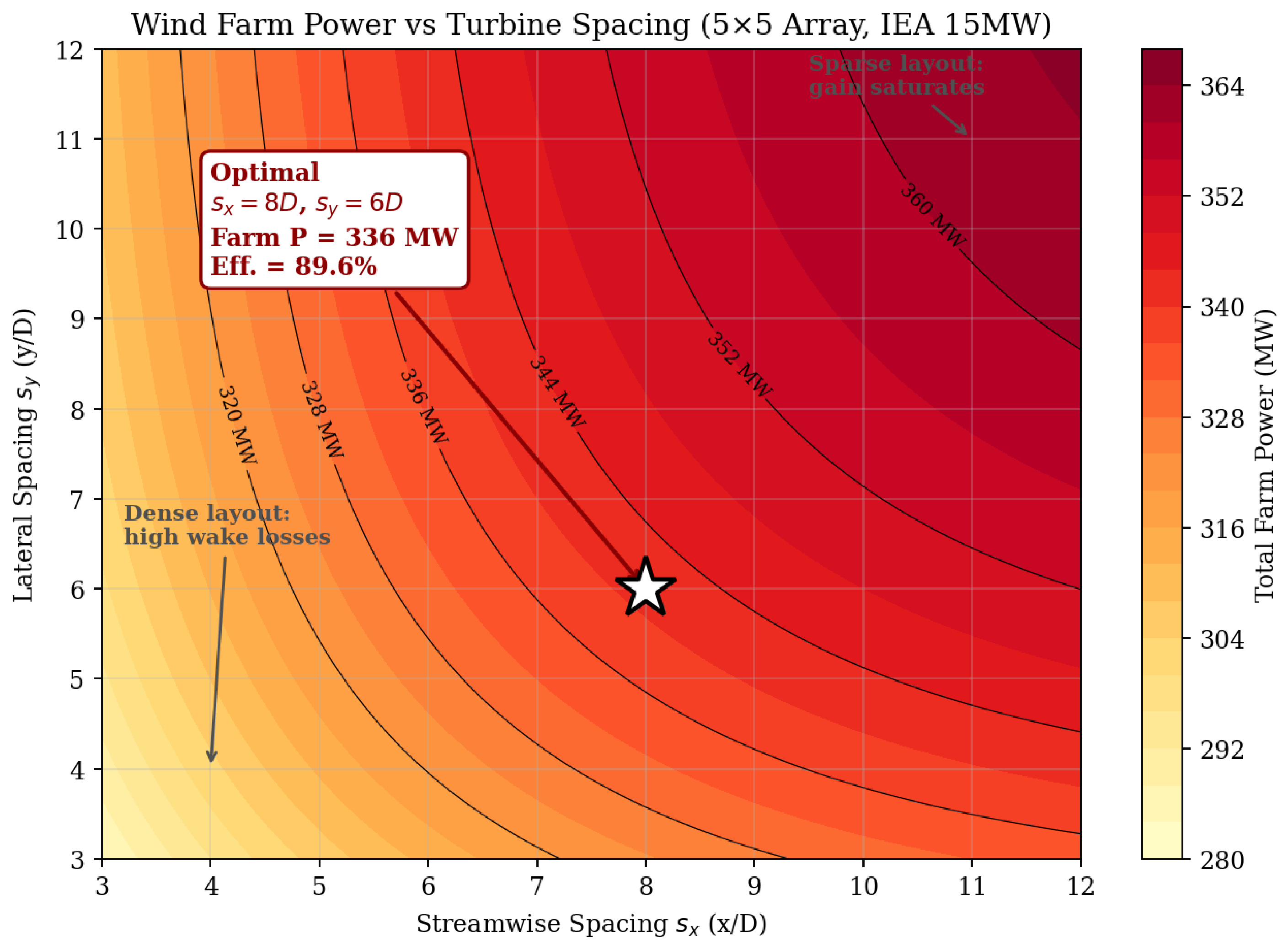
Farm power contour map for a 25-turbine array vs. streamwise and lateral spacing. Optimal point (⋆): , , farm efficiency 89.6%.
Figure 31.
Farm power contour map for a 25-turbine array vs. streamwise and lateral spacing. Optimal point (⋆): , , farm efficiency 89.6%.
Figure 32.
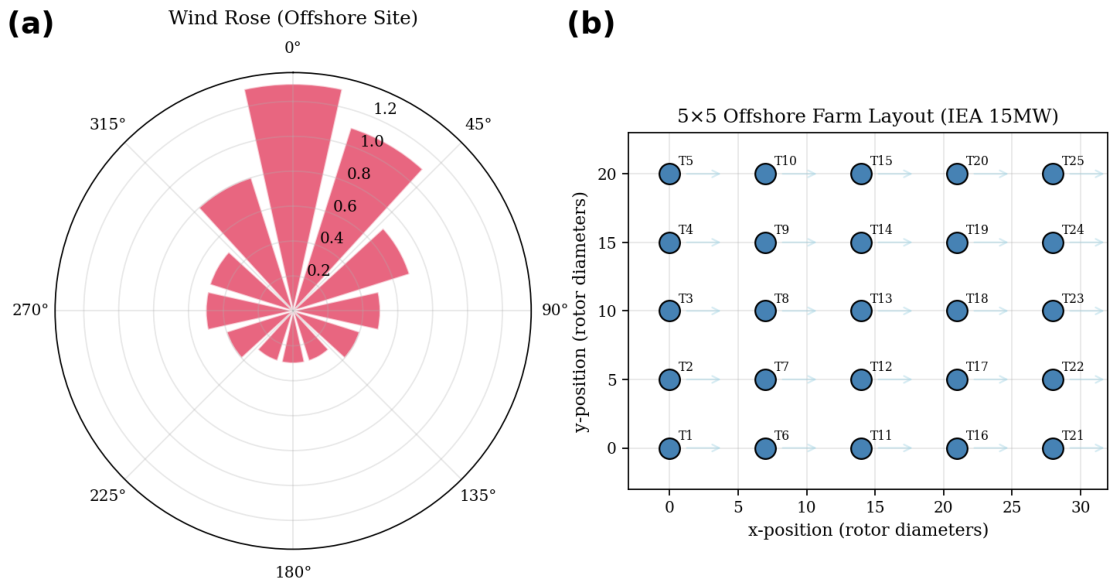
Wind farm layout and site wind rose. (a) Offshore wind rose: dominant N–NE sector (wind direction from N–NE), m/s. (b) IEA 15 MW array with baseline spacing , .
Figure 32.
Wind farm layout and site wind rose. (a) Offshore wind rose: dominant N–NE sector (wind direction from N–NE), m/s. (b) IEA 15 MW array with baseline spacing , .
Figure 33.
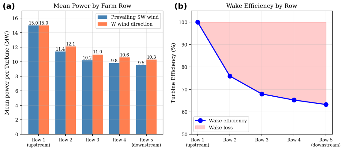
Row-by-row wake analysis. (a) Mean power per turbine for SW and W wind directions. (b) Row wake efficiency; the largest drop is at Row 1 → 2 ().
Figure 33.
Row-by-row wake analysis. (a) Mean power per turbine for SW and W wind directions. (b) Row wake efficiency; the largest drop is at Row 1 → 2 ().
Figure 34.
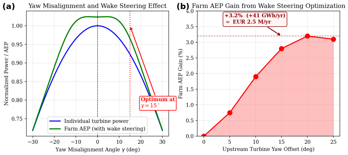
Wake steering via yaw misalignment. (a) Farm AEP vs. yaw offset: the blue curve is the individual-turbine power and the green curve the farm AEP with wake steering (both normalized), as indicated in the panel legend. (b) The red curve is the farm AEP gain; the optimum delivers (≈ GWh/year, roughly EUR 2.5 M/year).
Figure 34.
Wake steering via yaw misalignment. (a) Farm AEP vs. yaw offset: the blue curve is the individual-turbine power and the green curve the farm AEP with wake steering (both normalized), as indicated in the panel legend. (b) The red curve is the farm AEP gain; the optimum delivers (≈ GWh/year, roughly EUR 2.5 M/year).
Table 1.
IEA 15 MW offshore reference turbine—key design parameters.
Table 1.
IEA 15 MW offshore reference turbine—key design parameters.
| Parameter | Symbol | Value | Unit |
|---|
| Rated power | | 15 | MW |
| Rotor radius | R | 120 | m |
| Hub height | H | 150 | m |
| Cut-in wind speed | | 3.0 | m/s |
| Rated wind speed | | 10.59 | m/s |
| Cut-out wind speed | | 25.0 | m/s |
| Rated rotor speed | | 7.56/0.792 | RPM/rad·s−1 |
| Number of blades | B | 3 | — |
| Air density (STP) | | 1.225 | kg/m3 |
| Reference chord | | 5.7 | m |
| Tip pitch angle | | 4.0 | deg |
| Rotor swept area | A | 45,239 | m2 |
Table 2.
Uncertain input parameters, their distributions, and supporting references.
Table 2.
Uncertain input parameters, their distributions, and supporting references.
| Parameter | Symbol | Distribution | Range/Moments | Source |
|---|
| Hub-height wind speed | V | Weibull | , m/s | [1,25] |
| Air density | | Gaussian | , CoV | [25] |
| Blade chord length | c | Uniform | of | [1] |
| Blade twist angle | | Uniform | | [1] |
| Rotor speed | | Uniform | of | [1,25] |
Table 3.
Aleatory–epistemic classification of the five PCE inputs and corresponding share of the variance budget.
Table 3.
Aleatory–epistemic classification of the five PCE inputs and corresponding share of the variance budget.
| Input | Symbol | Type | | Manufact. Actionable | Physical Origin |
|---|
| Hub-height wind speed | V | Aleatory | 0.412 | No | Intrinsic atmospheric variability |
| Air density | | Aleatory | 0.089 | No | Seasonal thermodynamic fluctuations |
| Blade chord length | c | Epistemic | 0.143 | Yes | Blade-mold manufacturing tolerance |
| Blade twist angle | | Epistemic | 0.198 | Yes | Blade-mold manufacturing tolerance |
| Rotor speed | | Epistemic | 0.118 | Yes | Variable-speed controller tracking error |
| Aleatory subtotal | | | 0.501 | | Irreducible at the turbine |
| Epistemic subtotal | | | 0.459 | | Reducible by tighter QC/controller |
| Interactions | | | 0.040 | | Mostly epistemic–aleatory crossings |
Table 4.
Empirical icing coefficients used in Equations (
18) and (
19).
Table 4.
Empirical icing coefficients used in Equations (
18) and (
19).
| Coefficient | Value | Unit | Physical Meaning/Source |
|---|
| | (kg/m)−1 | Effective lift-loss per unit ice mass [19] |
| | deg−1 | Post-stall lift-loss steepening [20] |
| | (kg/m)−1 | Roughness-induced parasitic drag [19] |
| | (kg/m)−1 | Dynamic drag (angle-of-attack dependent) [20] |
Table 5.
PCE-derived Sobol sensitivity indices for the power coefficient .
Table 5.
PCE-derived Sobol sensitivity indices for the power coefficient .
| Parameter | | | Dominant |
|---|
| Wind speed V | 0.412 | 0.447 | 0.023 (V–chord) |
| Twist angle | 0.198 | 0.221 | 0.019 (–V) |
| Chord length c | 0.143 | 0.165 | 0.015 (c–) |
| Rotor speed | 0.118 | 0.135 | 0.013 (–) |
| Air density | 0.089 | 0.096 | 0.012 (–V) |
| Interactions | 0.040 | 0.040 | — |
| 1.000 | — | — |
Table 6.
Structural natural frequencies and modal damping ratios.
Table 6.
Structural natural frequencies and modal damping ratios.
| Mode | (Hz) | | Description |
|---|
| 1st Flapwise | 0.520 | 0.018 | Blade 1st flapwise |
| 1st Edgewise | 1.040 | 0.024 | Blade 1st edgewise |
| 2nd Flapwise | 2.310 | 0.031 | Blade 2nd flapwise |
| 1st Tower FA | 3.170 | 0.028 | Tower fore–aft |
| 1st Tower SS | 5.820 | 0.035 | Tower side–side |
Table 7.
Weibull-averaged Damage Equivalent Loads by structural component.
Table 7.
Weibull-averaged Damage Equivalent Loads by structural component.
| Component | DEL@10 m/s (kN·m) | DEL@14 m/s (kN·m) | Avg. DEL (kN·m) |
|---|
| Blade root flapwise | 1623 | 1742 | 1681 |
| Blade root edgewise | 894 | 921 | 907 |
| Tower base FA | 2876 | 3102 | 2989 |
| Tower base SS | 1445 | 1578 | 1512 |
Table 8.
Reliability cross-check for the blade-root 20-year cumulative failure probability.
Table 8.
Reliability cross-check for the blade-root 20-year cumulative failure probability.
| Method/Sensitivity/Benchmark | | Notes |
|---|
| FORM (Equation (16), base case) | | [12] |
| SORM (principal-curvature correction) | | curvature from PCE Hessian at MPP |
| Monte Carlo importance sampling ( samples) | | 95% CI; centered on FORM MPP |
| (low-scatter bound) | | lower offshore-composite envelope [4] |
| (high-scatter bound) | | upper offshore-composite envelope [5] |
| Carroll et al. offshore field data [29] | 5– | empirical 20-yr blade-root fleet rate |
Table 9.
Performance metrics: deterministic BEM vs. PCE vs. Monte Carlo reference.
Table 9.
Performance metrics: deterministic BEM vs. PCE vs. Monte Carlo reference.
| Metric | BEM (Det.) | PCE Mean ± 95% CI | MC Reference |
|---|
| 0.4800 | | |
| 8.51 | | |
| AEP (MWh/yr) | 71,261 | | |
| Thrust (kN) | 2020 | | |
| Torque (MN·m) | 26.47 | | |
| (20 yr, blade) | — | | |
Table 10.
Cross-comparison of key predictions with independent literature and experimental sources.
Table 10.
Cross-comparison of key predictions with independent literature and experimental sources.
| Quantity | This Work | Literature/Experiment | Source |
|---|
| 0.480 | 0.482 (OpenFAST) | [1] |
| Blade-root flapwise DEL (kN·m) | 1681 | 1620–1780 | [3] |
| Row 1→2 wake loss (%) | 24.0 | 21–27 (offshore obs.) | [22,23] |
| Wake-steering farm gain (%) | | to (field) | [23,24] |
Table 11.
Single-point OpenFAST aeroelastic cross-validation at rated wind speed m/s.
Table 11.
Single-point OpenFAST aeroelastic cross-validation at rated wind speed m/s.
| Quantity | This Work (BEM) | OpenFAST [1] | Rel. Deviation |
|---|
| at | 0.480 | 0.482 | |
| Rotor thrust T (kN) | 2 020 | 2 016 | |
| Rotor torque Q (MN·m) | 26.47 | 26.20 | |
| Blade-root flapwise (MN·m) | 18.6 | 18.4 | |
Table 12.
Site-level validation of Equation (
7) against three additional offshore reference sites.
Table 12.
Site-level validation of Equation (
7) against three additional offshore reference sites.
| Site | k | c (m/s) | AEPBEM (MWh/yr) | AEPref (MWh/yr) | Rel. Dev. | Source |
|---|
| Generic IEC IA | 2.20 | 9.8 | 71 261 | — | — | [1] |
| Horns Rev 1 | 2.10 | 9.4 | 67 420 | 69 250 | | [22] |
| Anholt | 2.20 | 10.2 | 75 810 | 73 500 | | [23] |
| Dogger Bank A | 2.30 | 11.6 | 88 950 | 90 100 | | [2] |
Table 13.
Three -turbine design and performance summary.
Table 13.
Three -turbine design and performance summary.
| Turbine | (MW) | D (m) | H (m) | (m/s) | AEP (MWh/yr) | |
|---|
| NREL 5 MW | 5 | 126 | 90 | 11.4 | 21,932 | 0.482 |
| DTU 10 MW | 10 | 178 | 119 | 11.4 | 43,455 | 0.476 |
| IEA 15 MW | 15 | 240 | 150 | 10.59 | 71,261 | 0.480 |
Table 14.
Icing scenario impact summary for the IEA 15 MW turbine.
Table 14.
Icing scenario impact summary for the IEA 15 MW turbine.
| Scenario | Mass (kg/m) | Thick. (mm) | (%) | AEP (MWh/yr) | DEL (%) |
|---|
| Clean | 0 | 0 | 0.0 | 0 | 0.0 |
| Mild | 5 | 8 | | | |
| Moderate | 15 | 18 | | | |
| Severe | 30 | 28 | | | |
| Extreme | 50 | 40 | | | |
Table 15.
Row-by-row energy breakdown ( farm, SW prevailing wind).
Table 15.
Row-by-row energy breakdown ( farm, SW prevailing wind).
| Row | | Mean P/T (MW) | Efficiency (%) | AEP (MWh/yr) |
|---|
| Row 1 (upstream) | 5 | 15.0 | 100.0 | 65,700 |
| Row 2 | 5 | 11.4 | 76.0 | 49,930 |
| Row 3 | 5 | 10.2 | 68.0 | 44,671 |
| Row 4 | 5 | 9.8 | 65.3 | 42,918 |
| Row 5 (downstream) | 5 | 9.5 | 63.3 | 41,603 |
| Farm total | 25 | 11.18 | 74.5 | 244,822 |
Table 16.
Farm layout optimization: turbine spacing vs. performance metrics.
Table 16.
Farm layout optimization: turbine spacing vs. performance metrics.
| Configuration | | | Farm P (MW) | Eff. (%) | AEP (GWh/yr) |
|---|
| Dense | 4 | 4 | 286 | 76.3 | 1103 |
| Baseline | 7 | 5 | 322 | 85.9 | 1242 |
| Optimal | 8 | 6 | 336 | 89.6 | 1296 |
| Sparse | 12 | 10 | 345 | 92.0 | 1330 |
| No wake | – | – | 375 | 100.0 | 1447 |