


Abstract
Accurate simulation of landfalling typhoons is essential for urban resilience in the densely populated Pearl River Delta. Using Super Typhoon Mangkhut (2018) as a case study, this paper evaluates the Weather Research and Forecasting (WRF) model through a contribution analysis designed to disentangle the roles of surface layer, planetary boundary layer (PBL), urban canopy model (UCM), and eddy-coefficient/diffusion closure parameterizations in wind-hazard prediction. Model results are validated against observations at the Hong Kong Observatory headquarters (HKO) and King’s Park (KP) stations, demonstrating that the hierarchy of physical controls is strongly metric-dependent. Substantial and structured spread is found among the tested configurations. Controlled comparisons show that PBL selection is the primary driver of variability in peak timing and high-wind persistence, whereas surface-layer formulation and diffusion closure exert secondary but systematic influences by shifting distributional centers and reshaping variability and upper tails. Urban canopy effects are comparatively weaker in aggregate but become more apparent during the impact and recovery phases. Overall, the results confirm that no single parameterization is consistently optimal across all metrics and motivate a multi-objective physics-selection strategy, in which multi-physics ensembles are used to better represent uncertainty in wind-event duration and associated loading risks in complex urban environments.
1. Introduction
The Northwest Pacific is the region with the most frequent tropical cyclone activity in the world, and these extreme weather events pose a major threat to coastal urban areas [1]. Typhoon Mangkhut, which occurred in 2018, demonstrated the devastating impact of strong typhoons on coastal urban areas, causing more than 458 injuries in Hong Kong and economic losses exceeding HK$4.6 billion in the city and approximately RMB 5.3 billion in southern China [2,3,4]. With the accelerating urbanization of coastal cities and the possible intensification of tropical cyclones under climate change, advanced modeling techniques are urgently needed to accurately assess the risk of typhoon-induced wind disasters in complex urban environments [4,5].
Previous studies have employed various methods to simulate typhoon wind fields and predict typhoon behavior. The WRF model is one of the most widely used mesoscale meteorological numerical models [6,7,8,9]. It can effectively predict and reproduce typhoon wind fields under real atmospheric conditions through advanced vortex bogusing and nested grid techniques. Davis et al. [6] demonstrated the capability of the Advanced Hurricane WRF model in predicting landfalling hurricanes, showing that systematic downscaling from coarse global data to 4 km resolution simulations performed as well as operational forecast systems. Hsiao et al. [10] developed a comprehensive vortex relocation scheme for tropical cyclone initialization in Advanced Research WRF, which addresses the challenge of weak or misplaced typhoon vortices in global analysis data through vortex separation, storm size correction, and intensity adjustment. The nested grid technique has proven particularly effective in WRF for multi-scale typhoon simulations, allowing systematic downscaling from synoptic-scale environmental flow to mesoscale typhoon dynamics [11,12,13]. Wu et al. [14] demonstrated through sensitivity analysis that two-way nesting configurations with progressive refinement from 30 km to 5 km resolution significantly outperformed single-domain simulations, particularly for typhoon intensity prediction. More recently, Wang et al. [15] developed a novel framework that combines WRF downscaling with pseudo-global warming techniques to assess climate change impacts on typhoon-induced urban wind fields, using Typhoon Mangkhut as a case study to demonstrate how future warming scenarios may alter typhoon wind field characteristics in urban environments. However, the performance of the WRF simulation strongly depends on the choice of physics parameterization schemes. In particular, boundary layer and surface-layer parameterizations can substantially modulate near-surface winds and intensity evolution, leading to notable inter-scheme variability [16,17]. Accurate prediction of sea-surface and coastal winds remains especially challenging, despite their critical roles in shaping coastal ocean environments and associated hazards. Although most planetary boundary layer (PBL) parameterizations are specifically designed to represent turbulent momentum transport and surface-layer coupling near the ground, many tropical-cyclone WRF studies still place greater emphasis on storm track, central pressure, and bulk near-surface wind statistics than on the systematic evaluation of hazardous winds at the lowest model levels, particularly over complex coastal and urban environments.
In WRF, the physics components are closely related through the representation of near-surface momentum exchange and boundary-layer turbulence [18,19,20]. The surface-layer scheme provides the lower-boundary fluxes by determining exchange coefficients, surface drag, and the coupling between the ground or sea surface and the atmosphere [21,22]. The PBL scheme then controls the vertical redistribution of momentum, heat, and turbulent kinetic energy, thereby affecting near-surface wind speed, vertical wind shear, and the persistence of strong winds [23,24]. Urban canopy models further modify the lower boundary over built-up areas by representing urban roughness, building drag, heat storage, and canopy-layer momentum loss [25]. In addition, eddy-diffusion or closure settings regulate subgrid-scale mixing and influence how rapidly momentum anomalies are smoothed, maintained, or dissipated [26]. Therefore, surface-layer, PBL, urban canopy, and diffusion parameterizations are not fully independent; instead, they form a coupled pathway through which WRF translates storm-scale forcing into local near-surface wind hazards [27,28]. Although previous studies have shown that these schemes can affect tropical cyclone track, intensity, and near-surface wind fields, their relative roles in shaping phase-dependent urban wind errors and peak wind persistence remain insufficiently quantified under a controlled comparison framework.
Existing studies have evaluated WRF simulations of tropical cyclones by comparing track and intensity against observations, and sensitivity tests of physics schemes have become a common practice [29,30,31]. Nevertheless, several gaps remain for extreme events and impact-oriented applications. First, wind verification is often limited to bulk error metrics (e.g., RMSE) and simple peak-value comparisons, rather than feature-oriented diagnostics of hazardous wind evolution. By contrast, local peak wind features that are more directly relevant to damage potential, such as the timing of peak wind occurrence, the duration of the peak-impact period, and the evolution of wind characteristics within that period, have been less systematically incorporated into reproducible verification frameworks. Second, while ensemble-based tropical cyclone studies often report forecast spread across models or physics options, fewer studies explicitly isolate how that spread arises from specific parameterization choices within a controlled sensitivity framework. In particular, the relative contributions of different scheme categories, such as boundary layer and surface layer parameterizations, are not always evaluated in a clearly attributable manner. Third, although observations from coastal and urban stations are increasingly used, the urban-modulated wind signal is not always isolated from other confounding factors, including track displacement; phase-dependent systematic discrepancies during the pre-typhoon, impact, and post-typhoon phases; station exposure and representativeness; and the coupling among surface-layer formulation, PBL parameterization, eddy-coefficient choices, and urban canopy treatments. Consequently, existing results often provide case-dependent rankings rather than transferable guidance on which physics components most directly control near-surface wind hazard characteristics in urban regions, motivating the controlled contribution analysis and multi-metric verification framework adopted in this study.
This study develops a comprehensive validation and parameter-contribution quantification framework for WRF simulations of Super Typhoon Mangkhut (2018) affecting Hong Kong, with a particular focus on how physics parameterizations shape track, intensity, and near-surface wind predictions. Specifically, this study (i) systematically compares 12 physics configurations (Base, Km1.5, PblMYNN, SfcMO, SfcMYNN, UrbBEP, UrbBEM, KmSMS, PblMYJ, PblYSU, KmSmsky, and PblBouLac) and quantifies their overall skill in reproducing typhoon track, intensity evolution, and near-surface wind speed time series against observations; (ii) complements conventional statistics with feature-oriented verification that targets typhoon peak-related behaviors, including peak timing, peak-impact wind duration, and wind speed evolution within the peak-impact window; (iii) quantifies scheme-induced variability by synthesizing cross-scheme dispersion and ranking consistency across multiple metrics, thereby revealing metric-dependent measurement standards (e.g., configurations that perform well for track may not be optimal for peak-impact wind characteristics) and identifying which aspects of the hazard are most sensitive to physics choices; and (iv) performs controlled, stage-resolved comparisons that isolate the effects of surface layer, PBL, UCM, and eddy coefficient with the Mangkhut lifecycle divided into the pre-typhoon phase, impact phase, and post-typhoon phase. This process-based, stage-dependent evaluation clarifies how scheme performance shifts across phases and links these shifts to evolving coastal wind hazards, thereby providing guidance for selecting physics configurations during operationally relevant impact periods.
The remainder of this paper is organized as follows: Section 2 briefly introduces the typhoon case study and presents the WRF model configuration, including domain setup, physical parameterization schemes, and urban surface representation. Section 3 describes the validation and comparative evaluation methodology using observational data from HKO and KP weather stations, including typhoon track accuracy, intensity evolution, and wind speeds at multiple locations. Section 4 discusses peak wind features, and the multi-objective decision implications for practical applications. Finally, Section 5 provides concluding remarks and the limitations.
2. Case Study and Physics Configurations
2.1. In Situ Measurements
Mangkhut was among the most powerful storms recorded in Hong Kong since 1946 [5,32,33]. The typhoon was accompanied by a pronounced low-level jet stream, which contributed to extensive economic losses and casualties across the southeastern coastal regions of China. Typhoon Mangkhut emerged over the northwest Pacific Ocean at 8:00 PM on 7 September 2018, and intensified into a super typhoon by 11 September. Early on 15 September, after hitting the northern Philippines, it moved into the South China Sea and made landfall in Haiyan Town, Taishan, Guangdong Province, at 5:00 PM on 16 September. Upon landfall, the typhoon had a maximum 10 min sustained wind speed near its center of 42–50 m/s, with the central pressure dropping to 95.5 kPa.
Wind speed validation was performed using observations from the HKO and KP stations, which represent two contrasting urban exposure conditions. The HKO station is located in the highly urbanized Tsim Sha Tsui area, and its wind observations are influenced by the surrounding dense built environment. The anemometer height is approximately 32 m above mean sea level. The location of HKO is 22°18′8″ N, 114°10′29″ E. KP is located on elevated hilly terrain. The station elevation is approximately 65 m above mean sea level, and the anemometer height is approximately 90 m above mean sea level. The KP Observatory is located at 22°18′42″ N, 114°10′21″ E. These two sites therefore provide complementary references for assessing model performance under different urban terrain and roughness conditions. The horizontal distance between HKO and KP is approximately 1.1 km based on their coordinates. In this study, the observed wind speeds were compared with the WRF diagnostic wind speed at the corresponding station observation/anemometer heights. No additional height or exposure correction was applied. Therefore, the wind speed differences reported here should be interpreted not only as model simulation errors but also as representativeness differences associated with station height, local terrain, building exposure, and unresolved urban roughness. This treatment is consistent with the objective of comparing the relative sensitivity of different WRF physics configurations under contrasting urban observational settings, rather than deriving a station-specific exposure-corrected wind estimate. Figure 1 shows the surrounding terrain and building distribution around the two observatories. This study validates and analyzes the numerical simulation results using the measured data from these two observatories during Typhoon Mangkhut (2018).
Figure 1.
The location of two observatories (copyright @ Maps of World: https://www.mapsofworld.com/answers/geography/what-are-the-key-facts-of-hong-kong-sar-china/attachment/hong-kong-map/# (accessed on 1 April 2026)).
2.2. Insert Bogus of Typhoon
The initial and lateral boundary conditions for WRF were derived from the ECMWF ERA5 reanalysis, using hourly pressure-level and surface fields at 0.25° × 0.25° resolution, which were preprocessed through the WPS system. Following the insertion of the Rankine vortex, the WRF model dynamically adjusts the vortex structure to ensure consistency with the surrounding environmental conditions defined by the ECMWF ERA5 fields [34,35]. The size and wind structure of the simulated cyclone are largely governed by the ambient large-scale conditions and the specific numerical schemes employed within the WRF framework [36]. To define the Rankine vortex, several key parameters must be specified, including the geographic coordinates of the cyclone center, the radius of maximum wind (RMW), and the maximum sustained wind speed [37]. The location (longitudes and latitudes) and intensity (central pressure and maximum wind speed) are typically derived from best track datasets provided by the Hong Kong Observatory. For this study, the historical track and intensity data of Typhoon Mangkhut were utilized. The RMW was estimated using the empirical relationships proposed by Chang et al. [38] and Liu et al. [39].
2.3. WRF Simulation Domain
The numerical experiments span from 0300 UTC on 15 September to 0300 UTC on 17 September 2018, corresponding to the period when Typhoon Mangkhut exhibited maximum wind intensity. The ERA5 reanalysis data with 0.25° × 0.25° resolution provides initial and boundary conditions for the WRF simulation. To accurately represent both large-scale atmospheric processes and local wind field characteristics, a five-level nested domain configuration is implemented. This computational framework utilizes progressively refined horizontal resolutions across five inter-nested domains to simultaneously resolve the synoptic-scale typhoon circulation and fine-scale urban wind structures. The horizontal grid spacing and domain sizes are as follows: Ad01 has a grid spacing of 8.1 km with 194 × 114 grid points; Ad02: 2.7 km, 34 × 37; Ad03: 0.9 km, 40 × 43; Ad04: 0.3 km, 58 × 61; and Ad05: 0.1 km, 103 × 111. Temporal resolution is adjusted proportionally across domains to maintain numerical stability and computational efficiency, with time steps ranging from 24 s in Ad01 to 0.30 s in Ad05. In the vertical direction, the atmosphere is discretized using 79 terrain-following levels extending from the near-surface atmosphere, approximately 1000 hPa, to the model top at 10 hPa. Following the terrain-following formulation of Laprise [40], the vertical grid is intentionally nonuniform, with enhanced resolution in the planetary boundary layer and gradual stretching aloft. This configuration improves the representation of near-surface wind shear and momentum exchange while avoiding excessive computational cost.
It should be noted that the innermost domains, especially Ad04 with 0.3 km grid spacing and Ad05 with 0.1 km grid spacing, fall within the turbulence gray zone between conventional mesoscale modeling and large-eddy simulation [41,42,43]. At these resolutions, part of the terrain-induced flow, urban heterogeneity, coastline effects, and larger turbulent or secondary circulation structures may become partially represented by the model-resolved dynamics. However, the PBL scheme still parameterizes subgrid vertical turbulent exchange, while the surface-layer and urban canopy schemes continue to parameterize surface fluxes, roughness effects, and canopy drag. Therefore, some overlap may exist between resolved and parameterized momentum transport and between partially resolved roughness effects and parameterized urban drag [44]. In this study, the inner nests are used as high-resolution mesoscale/urban-scale downscaling domains rather than true LES domains. Since all sensitivity experiments use the same nesting structure, the inter-configuration differences remain useful for evaluating the relative influence of physics parameterizations, but the absolute near-surface wind errors should be interpreted with this gray-zone limitation in mind.
2.4. Simulation Configuration
The physics options included in the model are the Kain–Fritsch (new-Eta) scheme [45,46] for cumulus parameterization, the Thompson scheme for microphysics [47,48], the RRTMG scheme [49] for long-wave and short-wave radiation transfer, and the Noah scheme [50] for land surface option. Twelve numerical simulations with different surface layer physics options, PBL boundary layer options, and urban canopy models (UCM) are conducted for each cyclone case, keeping all the other physics options fixed. The present sensitivity design focuses on the boundary-layer-related components that most directly regulate near-surface momentum exchange over coastal and urban areas. Therefore, microphysics, cumulus parameterization, radiation, land-surface model, and grid configuration were fixed across all experiments. Specifically, the Thompson microphysics scheme, Kain–Fritsch cumulus parameterization, RRTMG longwave and shortwave radiation schemes, Noah land-surface model, and the five-level nested grid configuration were kept unchanged. This design allows differences among simulations to be attributed primarily to the surface-layer formulation, PBL parameterization, UCM treatment, and eddy-diffusion/closure settings. The potential effects of the fixed model components are discussed later as part of the interpretation and limitations.
Table 1 summarizes the 12 WRF physics configurations, which were deliberately constructed following a one-factor-at-a-time (OFAT) controlled-comparison logic. In this design, one model option is changed at a time while the companion physics settings are held fixed. This provides a structured way to diagnose the sensitivity of the simulated track and near-surface winds to different parameterization choices. However, the term “controlled comparison” should not be interpreted as implying that these physical processes are fully independent. Surface-layer fluxes, urban canopy drag, PBL mixing, eddy diffusion, and grid-resolved near-surface variability are physically coupled, especially in the 0.3 km and 0.1 km inner domains. Therefore, the sensitivities discussed below are interpreted as effective, grid-conditioned responses under the selected nesting framework rather than as completely independent parameterization effects.
Table 1.
Physics parameterization scheme combinations.
(i) To examine the controlled sensitivity to surface-layer formulation, Base, SfcMO, and SfcMYNN share the same PBL (EEPS), SLUCM, and the horizontal Smagorinsky first-order closure and differ only in the surface layer formulation (revised MM5 Monin–Obukhov, Janjic Eta similarity, and MYNN, respectively). (ii) To examine the controlled sensitivity to PBL parameterization, Base, PblYSU, KmSMS and PblBouLac employ the same revised MM5 Monin–Obukhov surface layer, SLUCM, and horizontal Smagorinsky first-order closure, while the PBL scheme is switched among EEPS, YSU, no boundary layer and BouLac TKE. Complementarily, a second PBL-only contrast is provided by SfcMYNN versus PblMYNN, in which the MYNN surface layer is kept identical and only the PBL formulation changes (EEPS and MYNN), thereby testing whether the inferred PBL sensitivity is robust to surface-layer choice. (iii) To examine the controlled sensitivity to urban canopy representation, PblMYJ, UrbBEP, and UrbBEM keep the Janjic Eta similarity surface layer, MYJ (Eta) TKE PBL, and horizontal Smagorinsky first-order closure unchanged, while progressively increasing urban complexity from SLUCM to the multilayer BEP and BEM schemes. (iv) To diagnose the grid-conditioned sensitivity to eddy-diffusion/closure settings, Base, KmSmsky, and Km1.5 keep the revised MM5 Monin–Obukhov surface layer, EEPS PBL, and SLUCM unchanged while varying the turbulence closure among horizontal Smagorinsky first-order closure, Smagorinsky first-order closure, and a 1.5-order TKE closure. This comparison should not be interpreted as a grid-independent isolation of eddy-closure physics. Instead, it evaluates how different closure formulations behave within the selected nested-grid framework. In the 0.3 km and 0.1 km inner domains, some turbulent or secondary circulation structures may be partially resolved, while the closure schemes still parameterize subgrid-scale mixing. Therefore, the inferred eddy-closure sensitivity reflects the combined effect of grid resolution and closure formulation. Collectively, these OFAT groupings enable a structured comparison of how surface-layer physics, PBL parameterization, urban canopy representation, and grid-conditioned eddy-diffusion/closure settings affect track and near-surface wind differences. The resulting attribution is therefore conditional on the fixed nesting strategy and should not be interpreted as a grid-independent ranking of turbulence closures.
3. Validation and Comparative Evaluation of Physics Configurations
3.1. Validation Metrics
Observational validation data were obtained from the HKO and KP meteorological stations, which provide high-quality, 10 min averaged wind speed and wind direction measurements. To evaluate the performance of the WRF-simulated typhoon wind fields, four statistical metrics, as shown in Equations (1) and (2), are employed: root mean square error (RMSE), mean absolute error (MAE), and the minimum or maximum error, where and represent simulated and observed values at stage, respectively, and is the sample size. Using MAE and RMSE together can provide complementary information. Specifically, MAE summarizes the average performance, whereas RMSE highlights whether the simulation shows intermittent but substantial outliers. In this study, lower MAE/RMSE indicates better agreement; additionally, cases with comparable MAE but noticeably higher RMSE are interpreted as having similar errors but more frequent or more severe extreme errors. To support the contribution analysis more quantitatively, an error-increment metric was further introduced for each controlled comparison group. For a given metric E, such as track MAE, intensity MAE, or phase-specific wind-speed MAE, the error increment caused by changing one physics component is defined as Equation (3), where is the error metric of the perturbed configuration and is the corresponding reference configuration within the same one-factor-at-a-time group. A positive indicates degradation relative to the reference case, whereas a negative indicates improvement.
3.2. Track
For track verification, the instantaneous track error is defined as the absolute distance between the simulated typhoon center and the observed best-track center at the same time. The observed typhoon center is obtained from the best-track data. Lower values indicate better agreement between the simulated and observed tracks. Table 2 and Figure 2 summarize the track-error statistics for the 12 configurations and shows a structured but not uniformly large spread in trajectory performance. Rather than supporting a strict best-to-worst ranking, the completed simulations separate into a relatively compact leading group, a broader mid-field, and a distinctly weaker tail. UrbBEM yields the smallest reported track errors (MAE = 20.1 km; RMSE = 21.6 km; max error = 36.2 km), but this apparent advantage must be interpreted with caution because the simulation terminated early and therefore covers only a shorter segment of the 48 h event (stopped at 0640 UTC 16 September). For that reason, UrbBEM cannot be treated as directly comparable with the fully completed runs in a full-period ranking framework. Among the simulations that completed the full integration, PblMYNN provides the lowest mean errors (MAE = 21.1 km; RMSE = 23.9 km), although its max error remains relatively larger (57.5 km), indicating that it improves typical track performance while still allowing a few noticeable excursions. A compact mid-performance cluster includes SfcMO, SfcMYNN, UrbBEP, Km1.5, KmSMS, PblMYJ, and Base, with MAE values of 22.3–25.6 km and RMSE values of 24.6–28.0 km. In contrast, PblYSU already represents a clear degradation (31.2/36.9 km), while KmSmsky and especially PblBouLac form a distinct weak tail (33.6/42.0 km and 42.5/55.5 km, respectively). Thus, the main conclusion of Table 2 and Figure 2 is not that one configuration is universally “best”, but that physics choices alone can generate an organized and physically meaningful spread in track behavior under the same storm initialization and domain setup.
Table 2.
Track performance conclusion of 12 simulation configurations.
Figure 2.
Simulated vector tracks from the 12 configurations are presented together with the Hong Kong Observatory (HKO) observational track for Typhoon Mangkhut.
Using the one-factor-at-a-time design in Table 1, the track spread can be interpreted more mechanistically. When only the surface layer is changed while PBL (EEPS), UCM (SLUCM), and eddy closure are held fixed, both SfcMO and SfcMYNN improve upon Base. The MAE/RMSE decreases from 25.6/28.0 km in Base to 22.3/24.6 km in SfcMO and 22.8/25.2 km in SfcMYNN. The corresponding maximum absolute track error also declines from 51.6 km to 46.3–47.1 km. This indicates that the near-surface flux formulation exerts a consistent but moderate control on track skill. However, the effect becomes much larger when the PBL scheme is changed. Under the MYNN surface layer pair, switching from EEPS (SfcMYNN) to MYNN (PblMYNN) reduces MAE/RMSE from 22.8/25.2 km to 21.1/23.9 km but also increases the max error from 47.1 km to 57.5 km, implying improved average behavior but greater tail risk. Under the revised-MM5 family, changing Base to PblYSU degrades MAE/RMSE from 25.6/28.0 km to 31.2/36.9 km and increases max error from 51.6 km to 71.5 km, while switching to PblBouLac causes a much stronger deterioration (42.5/55.5 km; max error = 111.0 km). A similar degradation appears under the MO surface layer, where PblMYJ is clearly worse than SfcMO (24.8/27.1 km and 22.3/24.6 km).
PBL parameterization can affect track indirectly by modifying the internal structure of the tropical cyclone and its coupling to the environmental steering flow. Different PBL schemes regulate the strength and depth of low-level radial inflow, the vertical transport of angular momentum, and the distribution of near-surface winds. These processes can alter the compactness of the vortex and the radius of maximum wind, thereby changing the storm’s inner-core structure. At the same time, the PBL scheme controls how surface heat, moisture, and momentum fluxes are mixed upward, which can influence eyewall convection and the maintenance of the vortex core. By determining the depth of the inflow layer and the efficiency of turbulent momentum exchange, the PBL scheme can further affect the vertical coherence of the vortex. A vortex with different vertical coupling may interact differently with the deep-layer environmental steering flow, leading to different simulated track displacements. Therefore, the larger track-error spread associated with PBL changes in this study is physically consistent with an indirect pathway in which boundary-layer mixing reshapes the storm structure and its steering-flow coupling, whereas surface-layer changes mainly provide a smaller adjustment through near-surface drag and flux coupling. Because the present study focuses on track, intensity, and near-surface wind verification rather than a full inner-core budget analysis, this mechanism is used here to interpret the scheme-dependent behavior rather than to claim a complete causal decomposition of the track error. Future work should explicitly diagnose radial inflow, inflow-layer depth, radius of maximum wind, diabatic heating, and vortex tilt to further quantify this pathway.
The UCM and eddy-closure contrasts provide additional information. Within the MYJ-based family, moving from SLUCM (PblMYJ: 24.8/27.1 km; max error = 55.2 km) to BEP (UrbBEP: 23.7/26.1 km; 48.3 km) and then to BEM (UrbBEM: 20.1/21.6 km; 36.2 km) suggests that more detailed urban representation can improve track behavior for a storm interacting with a dense coastal city. However, because UrbBEM did not complete the full simulation, this apparent benefit should be interpreted as case-specific support for the importance of land-surface representation, not as a definitive endorsement of BEM. The eddy-closure family also shows that not all diffusion choices are benign. Km1.5 remains close to Base in MAE/RMSE (24.3/26.9 km and 25.6/28.0 km), whereas KmSmsky degrades sharply to 33.6/42.0 km and increases max error to 91.1 km. Overall, the controlled comparisons indicate that PBL and eddy-diffusion choices exert the largest leverage on track performance in this case; the UCM provides a potentially beneficial but case-specific adjustment, and the surface layer contributes a smaller but systematic shift.
3.3. Intensity
Figure 3 shows the time series of the central-pressure difference (simulation minus observation, hPa) for the 12 configurations from 0300 UTC 15 September to 0300 UTC 17 September All configurations share a common first-order temporal structure. A positive central-pressure error indicates that the simulated central pressure is higher than observed, corresponding to an under-deepened and therefore weaker simulated typhoon. A negative value indicates that the simulated central pressure is lower than observed, corresponding to an overly deepened simulated typhoon. Since minimum central pressure is used here as the intensity indicator, the central-pressure bias is also referred to as the pressure-based intensity bias. The bias remains persistently positive during most of 15 September, increases toward a peak around early 16 September, and then decreases coherently toward small or even slightly negative values by the end of the simulation. This behavior agrees with previous tropical-cyclone modeling studies showing that the intensity evolution is largely constrained by the storm lifecycle and large-scale forcing, whereas PBL and related physics schemes mainly modulate the magnitude and persistence of the intensity bias through turbulent momentum transport, boundary-layer inflow, surface flux coupling, and convective organization [51,52,53]. In the present Mangkhut simulations, the coherent temporal pattern shared by all configurations therefore reflects the common storm-evolution signal, while the inter-scheme spread indicates how different physics choices regulate the simulated vortex intensity within that shared large-scale framework. Among the configurations, SfcMO produces the smallest peak deviation in Figure 3 (25.6 hPa), and several schemes, such as Km1.5, KmSMS, PblMYNN, PblYSU, SfcMO, SfcMYNN, and Base, briefly cross into slightly negative values late in the simulation. The key point, however, is not the exact ordering of all curves but that most schemes show a persistent under-deepening tendency over an extended period and differ mainly in how strongly and how long that bias is maintained. This behavior is consistent with previous tropical-cyclone modeling studies [53,54]. Physically, excessive vertical mixing can over-distribute momentum through an overly deep boundary layer, weaken low-level radial inflow and angular-momentum convergence near the radius of maximum wind, suppress eyewall ascent and convective organization, and ultimately limit warm-core development and pressure deepening.
Figure 3.
Typhoon central-pressure difference (hPa) across 12 configurations for Typhoon Mangkhut, and the SfcMO has the lowest maximum pressure deficit (25.6 hPa).
Table 3 condenses this behavior into MAE and RMSE. Among the completed runs, SfcMO performs best (MAE/RMSE = 14.6/15.9 hPa), followed closely by PblMYNN (14.9/16.4 hPa). A compact middle group includes Base (15.5/16.9 hPa), Km1.5 (15.6/16.9 hPa), KmSMS (15.8/17.1 hPa), SfcMYNN (15.9/17.4 hPa), PblYSU (16.0/17.3 hPa), UrbBEP (16.1/17.2 hPa), and PblMYJ (16.4/17.5 hPa). More evident degradation appears for PblBouLac (17.8/18.5 hPa) and especially KmSmsky (18.8/19.6 hPa), which form the weaker tail among the completed simulations. UrbBEM reports the largest central-pressure error (20.0/20.1 hPa), but because this simulation terminated before 48 h, it is not included in the full-period ranking interpretation. In Table 3, RMSE is only slightly larger than MAE for most configurations. This small difference suggests that the central-pressure errors are dominated by a persistent systematic component, rather than by a few isolated large deviations, which is consistent with the extended positive central-pressure bias shown in Figure 3.
Table 3.
Central-pressure difference performance conclusion of 12 simulation configurations.
The one-factor-at-a-time comparisons clarify why the scheme ranking changes less dramatically for intensity than for track, while still remaining physically meaningful. When only the surface layer is varied under fixed EEPS PBL and SLUCM, SfcMO improves upon Base (14.6/15.9 and 15.5/16.9 hPa), whereas SfcMYNN is slightly worse (15.9/17.4 hPa). This suggests a measurable but moderate sensitivity to surface-layer formulation, with an MAE spread of about 1–1.5 hPa. The PBL contrasts are more influential. Under the MYNN surface layer, changing from EEPS (SfcMYNN: 15.9/17.4 hPa) to MYNN (PblMYNN: 14.9/16.4 hPa) improves both metrics by about 1 hPa. Under the revised-MM5 family, changing from EEPS (Base: 15.5/16.9 hPa) to YSU (PblYSU: 16.0/17.3 hPa) causes only mild degradation, but switching to BouLac (PblBouLac: 17.8/18.5 hPa) worsens MAE by 2.3 hPa. Likewise, under the MO surface layer, replacing EEPS (SfcMO) with MYJ (PblMYJ) degrades MAE from 14.6 hPa to 16.4 hPa. The UCM effect is weaker and not monotonic: PblMYJ improves slightly to UrbBEP (16.1/17.2 hPa), whereas UrbBEM degrades strongly (20.0/20.1 hPa), although that result is confounded by incomplete simulation. The eddy-controlled family also shows a sharp contrast: Km1.5 remains close to Base (15.6 and 15.5 hPa), while KmSmsky degrades to 18.8/19.6 hPa. Taken together, these results suggest that, within the fixed microphysics, cumulus, radiation, land-surface, and grid-resolution settings used in this study, the inter-configuration differences in central-pressure bias are mainly associated with how each boundary-layer and diffusion configuration sustains the vortex core through vertical mixing, turbulent diffusion, momentum exchange, and surface-flux coupling. Physically, overly strong vertical mixing can redistribute momentum through a deeper boundary layer, weaken the near-surface wind maximum, reduce low-level radial inflow, and decrease angular-momentum convergence near the radius of maximum wind. These changes can weaken eyewall ascent and convective organization, limit warm-core development, and therefore reduce pressure falls. The PBL influence should also not be interpreted independently of the surface layer, because surface momentum exchange controls frictional dissipation and inflow forcing, whereas enthalpy exchange regulates the heat and moisture supply available for eyewall convection.
This interpretation should not be taken to imply that microphysics, convection parameterization, or grid resolution are unimportant for typhoon intensity. Microphysics can affect latent heat release, precipitation structure, and eyewall or rainband organization; cumulus parameterization can influence convective heating and large-scale vortex adjustment, especially in the coarser outer domains; and grid resolution controls the degree to which storm structure, topography, urban roughness, and turbulent motions are explicitly resolved. These factors may influence the absolute magnitude of the central-pressure error, but because they are held fixed in the present OFAT design, they are not responsible for the relative spread among the tested boundary-layer-related configurations.
3.4. Wind Speed
The temporal evolution of wind speeds during Typhoon Mangkhut shows distinct patterns across different stages of development. To better assess scheme performance, the wind speed evolution is divided into three phases: (1) a pre-typhoon phase, (2) a typhoon impact phase, and (3) a post-typhoon phase. This phase definition is based on the storm’s distance to the site of interest (Hong Kong in this study) using a 200 km radius threshold [55,56]. Specifically, the pre-typhoon phase corresponds to the period when the typhoon center remains outside the 200 km circle; the impact phase covers the period when the typhoon center is within 200 km of Hong Kong, during which the strongest and most severe winds typically occur; and the post-typhoon phase begins once the typhoon center moves beyond the 200 km radius again. This division enables a systematic evaluation of how well the mesoscale model reproduces the time history of sustained winds at fixed locations, while also highlighting its limitations during the peak-impact period. The following analysis presents the performance of different schemes in each phase, with statistical metrics summarized in the accompanying tables.
3.4.1. HKO
- (1)
- Pre-typhoon phase
Figure 4a shows that all simulations show a coherent and systematic positive bias relative to HKO during the pre-typhoon phase. The observed 10 min mean wind remains low and increases gradually, whereas nearly all configurations predict earlier strengthening and a higher background wind level. Table 4 confirms that the pre-phase bias is uniformly positive and typically falls in the range of about 5–9 m/s, indicating that the dominant error mode is a persistent early-onset overestimation rather than isolated spikes. Among the tested configurations, Base provides the smallest pre-phase errors (Bias/MAE/RMSE = 5.7/5.7/6.1 m/s), while SfcMO and SfcMYNN are slightly worse but still relatively close (both MAE = 6.5 m/s). By contrast, PBL-related alternatives produce a larger spread, with PblYSU reaching 7.8/7.8/8.6 m/s and PblBouLac reaching 8.9/8.9/9.8 m/s. The MYJ-based UCM family shows only small differences at this stage, with PblMYJ, UrbBEP, and UrbBEM all remaining near 7.2–7.4 m/s MAE, while the eddy-closure group indicates a non-negligible sensitivity: relative to Base, Km1.5, KmSMS, and KmSmsky increase MAE to 6.7, 7.4, and 6.7 m/s, respectively.
Figure 4.
Ten-minute average wind speed from observation and simulation at the HKO station. (a) Pre-typhoon phase; (b) impact phase; (c) post-typhoon phase.
Table 4.
Statistical performance metrics for 12 configurations compared with HKO observations across typhoon stages.
The more important interpretation is that the pre-typhoon phase already reveals an early-onset problem rather than only a magnitude problem. The model strengthens the near-surface wind too early, indicating that HKO is affected by a simulated outer wind field that is too strong, too broad, or too efficiently projected downward before the storm core arrives. In such a situation, the local low-level vertical momentum gradient may be overestimated because stronger winds above the surface are available to be mixed downward into the frictional layer. The PBL scheme is therefore a key control on this error pathway: by determining the depth, diffusivity, and efficiency of turbulent momentum exchange, it regulates how rapidly high-momentum air aloft is transported toward the near-surface layer. Excessive or overly efficient mixing can initiate surface-wind strengthening earlier than observed, producing the persistent positive bias seen during the pre-typhoon phase. Within the one-factor-at-a-time framework, this explains why PBL parameterization produces the largest change in early-phase HKO errors, followed by eddy closure, while the surface layer exerts a smaller but still systematic influence through surface drag and flux coupling.
- (2)
- Typhoon impact phase
During the impact phase in Figure 4b, the observation rises into a high-wind plateau with strong temporal variability, whereas the simulations diverge much more strongly than in the pre-phase in both peak magnitude and post-peak persistence. Table 4 shows that this is the most discriminating period, with RMSE ranging from about 3.9 to 11.4 m/s. Among the completed runs, Base and SfcMYNN form the leading group (Base: 1.1/3.1/3.9 m/s; SfcMYNN: 2.8/3.2/4.4 m/s). Km1.5 (MAE = 3.7 m/s) and KmSmsky (3.5 m/s) remain moderately close, whereas KmSMS degrades more clearly (5.5/5.5/6.6 m/s). The PBL-related departures become much larger during impact: PblMYJ, PblMYNN, and PblYSU all have MAE values around 6.2–6.7 m/s, while PblBouLac reaches 10.6/10.6/11.4 m/s. The UCM effect becomes more visible in this high-wind window. Within the MYJ-based group, UrbBEM (4.4/5.7/7.4 m/s) improves noticeably relative to PblMYJ (6.6/6.7/7.8 m/s), whereas UrbBEP (6.8/6.9/8.0 m/s) remains close to PblMYJ, indicating that urban effects are configuration-dependent in both sign and magnitude.
This phase shows most clearly that the HKO’s error is not simply a peak-amplitude bias but a persistence bias. Several schemes maintain strong winds for too long and decay too slowly after peak passage. The one-factor-at-a-time contrasts indicate that PBL choice remains the dominant lever because it can increase MAE from 3.1 m/s in Base to 6.7 m/s in PblYSU and up to 10.6 m/s in PblBouLac under otherwise comparable settings. The surface-layer contribution also becomes more pronounced in this phase: under EEPS, SfcMO has MAE = 5.4 m/s and 3.1 m/s for Base, whereas SfcMYNN remains much closer to Base. Eddy-closure choices act as a secondary control, ranging from mild perturbation (Km1.5) to more obvious degradation (KmSMS).
Physically, this suggests that high-wind performance at the HKO depends not only on the magnitude of momentum transfer but also on the time-dependent adjustment of the near-surface winds during storm-core passage. During the impact phase, the strong pressure-gradient force, intense low-level vertical shear, and enhanced turbulence production create a rapidly evolving boundary layer. The PBL formulation mainly controls two aspects of this process: the intensity of vertical turbulent mixing and the depth of the boundary layer. The former determines how efficiently high-momentum air from stronger winds aloft is mixed downward toward the near-surface layer, directly influencing near-surface wind speed. The latter determines the vertical depth over which momentum, turbulence, and surface-friction effects are redistributed, thereby affecting the adjustment and spin-down timescale of the near-surface wind field. At the same time, radial inflow and radial advection control how high-momentum air within the vortex is transported toward and across the station. If the PBL scheme produces overly efficient, overly deep, or overly persistent mixing, the near-surface winds can strengthen too rapidly and remain elevated for too long, producing the persistence bias seen in several configurations. As the storm moves away and the pressure-gradient forcing weakens, the local wind field must spin down; the decay rate then depends on the combined effects of vertical mixing efficiency, boundary-layer depth, surface drag, turbulent diffusion, and the weakening of radial momentum advection. Therefore, the impact-phase differences among the configurations are interpreted as the combined result of PBL-controlled mixing intensity, boundary-layer depth, vertical momentum redistribution, and radial-advection effects, while the surface layer and eddy closure provide secondary modulation through surface drag, flux coupling, and turbulent diffusivity.
- (3)
- Post-typhoon phase
In the post-typhoon period, as shown in Figure 4c, the observed wind speed drops to a lower regime, while many simulations retain elevated winds and therefore show a slow-decay tendency. Table 4 again shows positive bias across all reported schemes, indicating that the dominant post-impact error is an overly slow relaxation. Base remains the most accurate completed configuration (3.4/3.6/4.3 m/s), followed by SfcMYNN (4.7/4.7/5.4 m/s). The eddy-closure family is systematically worse than Base in this phase, with Km1.5, KmSMS, and KmSmsky yielding MAE values of 5.1, 5.2, and 5.4 m/s, respectively. The PBL-driven degradations remain stronger, with PblMYNN, PblYSU, and PblBouLac increasing MAE to 6.0, 6.3, and 7.6 m/s. The UCM effect is comparatively small in the available comparisons: UrbBEP (5.2/5.5/6.4 m/s) remains close to PblMYJ (5.7/5.7/6.5 m/s), and UrbBEM is not available in the post-phase statistics because the simulation ended early.
The post-phase therefore reinforces the same physical interpretation as the impact phase: the key difference among configurations is how quickly the near-surface momentum reservoir is dissipated after the strongest forcing has passed. Relative to Base (MAE = 3.6 m/s), switching the PBL to YSU or BouLac increases MAE by about 2.7–4.0 m/s, while changing the eddy closure to KmSmsky increases MAE by about 1.8 m/s. Surface-layer differences remain secondary but still visible, as shown by the contrast between Base and SfcMO (3.6 and 5.9 m/s) and between Base and SfcMYNN (3.6 and 4.7 m/s). Overall, the HKO results are most usefully interpreted as evidence that physics choices strongly reshape the duration and relaxation of hazardous winds, not merely their peak value.
Across all three phases, the simulations share a consistent tendency toward positive wind speed bias at HKO, but the relative importance of the controlling physics changes with storm evolution. PBL parameterization is the dominant factor in every phase and is also the clearest discriminator between the leading group and the weaker tail, with PblBouLac consistently producing the largest errors (pre: MAE = 8.9 m/s; impact: 10.6 m/s; post: 7.6 m/s). The eddy closure is secondary in the pre-phase, becomes phase-dependent during impact, and again grows in importance in the post-phase, where decay behavior is especially sensitive to diffusion settings. Surface-layer effects are detectable throughout but are most consequential during impact, while UCM effects remain weakest overall at HKO, although some UCM choices can still modify peak-phase errors under otherwise fixed settings. Thus, HKO does not mainly identify a single universally optimal scheme; instead, it shows that the dominant model error is a timing-and-persistence error whose amplitude is controlled primarily by the PBL framework.
The phase-dependent wind speed bias can be interpreted as a balance between boundary-layer momentum transport and large-scale typhoon forcing. During the pre-typhoon phase, observed near-surface winds are still relatively weak, whereas some simulations strengthen too early. This early positive bias can result from small errors in storm approach timing and from PBL schemes that mix stronger low-level momentum downward too efficiently before the main typhoon impact reaches HKO. During the impact phase, the wind field is more strongly constrained by the typhoon-scale pressure-gradient force and organized cyclonic circulation. Therefore, the mean signed bias can become smaller for some configurations because both observations and simulations are within the high-wind regime, although MAE, RMSE, and persistence errors may still remain significant. During the post-typhoon phase, the observed wind speed decreases rapidly as the large-scale forcing weakens, while many simulations retain elevated winds for too long. This suggests an overly persistent boundary-layer momentum reservoir and insufficiently rapid dissipation of storm-induced low-level momentum. Thus, the larger pre- and post-phase biases are mainly associated with transition-period sensitivity to boundary-layer mixing, vertical momentum transport, and local exposure effects, whereas the impact phase is more directly dominated by large-scale typhoon forcing.
3.4.2. KP
- (1)
- Pre-typhoon phase
Figure 5a shows that before the closest approach, the KP observation remains comparatively low, while nearly all simulations start from a higher background level and intensify too early. The inter-scheme spread is moderate at first but increases steadily as the event approaches. Table 5 confirms that the bias is positive and close to MAE for almost all schemes, indicating that the dominant pre-phase discrepancy is a persistent offset rather than a random fluctuation. Base again provides the smallest error (bias/MAE/RMSE = 3.5/3.6/4.1 m/s), whereas most other configurations cluster between about 5 and 6.6 m/s in MAE, including SfcMO (5.1/5.1/5.8), SfcMYNN (5.1/5.1/5.7), Km1.5 (5.4/5.4/6.0), and PblYSU (6.6/6.6/7.3). PblBouLac is among the weakest cases (7.1/7.1/7.9 m/s).
Figure 5.
Ten-minute average wind speed from observation and simulation at the KP station. (a) Pre-typhoon phase; (b) impact phase; (c) post-typhoon phase.
Table 5.
Statistical performance metrics for 12 configurations compared with KP observations across typhoon stages.
Within the one-factor-at-a-time grouping, the pre-phase KP errors again indicate that PBL choice and eddy closure are the strongest levers, while surface-layer and UCM effects are secondary. Relative to Base (MAE = 3.6 m/s), changing only the surface layer increases MAE to 5.1 m/s for both SfcMO and SfcMYNN. Changing the eddy closure produces similarly large shifts, with Km1.5, KmSMS, and KmSmsky reaching 5.4, 6.1, and 5.6 m/s, respectively. The PBL differences are larger still: PblYSU increases MAE to 6.6 m/s and PblBouLac to 7.1 m/s. The urban-canopy upgrade has a smaller but consistent influence within the MYJ family, where PblMYJ (MAE = 6.0 m/s) improves to UrbBEP (5.2 m/s) and UrbBEM (5.4 m/s). Compared with HKO, KP already suggests that the inland station is more sensitive to how the model projects background momentum into the local near-surface layer even before peak forcing begins.
- (2)
- Impact phase
In Figure 5b, the KP observation reaches its strongest winds but also shows pronounced temporal variability, including a marked drop that many simulations fail to reproduce. Most configurations instead maintain a much higher and flatter high-wind plateau. Table 5 confirms that the impact phase is the most challenging regime for KP, with MAE ranging from 4.5 m/s in Base to 14.5 m/s in PblBouLac. Base remains the leading completed configuration (bias/MAE/RMSE = 4.2/4.5/5.1 m/s), whereas a middle group includes KmSmsky (6.8/6.8/7.4), UrbBEM (7.2/7.2/9.1), and SfcMYNN (7.6/7.6/8.2). Stronger degradation is concentrated in the PBL variants that sustain excessive high winds during peak conditions, including PblMYJ (11.5/11.5/12.0), PblMYNN (11.5/11.5/12.0), PblYSU (11.6/11.6/12.0), and especially PblBouLac (14.5/14.5/15.2). The fact that bias is again close to MAE across most cases indicates that this discrepancy is primarily systematic overestimation, not just intermittent spikes.
The one-factor-at-a-time contrasts show that PBL choice dominates the impact-phase outcome, but they also reveal that KP is more responsive than HKO to urban representation. Under otherwise comparable settings, changing the PBL from Base to PblYSU or PblBouLac raises MAE from 4.5 m/s to 11.6 and 14.5 m/s, while the MYNN pair shows a similar deterioration from SfcMYNN (7.6 m/s) to PblMYNN (11.5 m/s). Within the MYJ-based urban family, the UCM effect is amplified under impact conditions: PblMYJ (11.5 m/s) improves to UrbBEP (9.0 m/s) and further to UrbBEM (7.2 m/s). Surface-layer effects are also substantial at KP, as shown by Base and SfcMO (4.5 and 8.9 m/s), and eddy-closure differences remain large (Base 4.5; Km1.5 8.4; KmSMS 9.8 m/s), but both are generally smaller than the most severe PBL-driven departures.
This pattern suggests that KP is especially sensitive to the PBL-controlled adjustment of near-surface winds during peak passage. Strong pressure-gradient forcing and intense low-level shear create large vertical momentum gradients, and the PBL scheme determines how efficiently turbulent vertical momentum flux mixes high-momentum air downward. If this mixing is too deep or too persistent, the simulated near-surface winds may remain elevated even after the observed winds begin to weaken, producing a high-wind plateau that is too strong and too persistent. This adjustment is further modulated by radial momentum advection, surface drag, and eddy diffusivity. Therefore, the KP impact-phase bias is interpreted as a time-dependent near-surface wind adjustment problem rather than only a peak-magnitude error.
- (3)
- Post-phase
Figure 5c shows that after the storm core passes, the KP observation drops substantially and remains relatively suppressed, whereas most simulations decay too slowly and keep winds elevated for too long. The spread is smaller than in the impact phase but the positive bias persists. Base again performs best among the completed runs (4.7/4.9/5.7 m/s), and SfcMYNN remains relatively competitive (6.1/6.3/7.2 m/s). In contrast, the PBL-driven cases remain clearly worse, including PblMYNN (7.2/7.2/7.6), PblMYJ (8.6/8.6/8.9), PblYSU (8.7/8.7/8.9), and PblBouLac (9.8/9.8/10.1). The UCM comparison available here suggests moderate improvement from BEP relative to the SLUCM baseline in the MYJ family (UrbBEP: 7.4/7.4/8.0 and PblMYJ: 8.6/8.6/8.9), while UrbBEM is unavailable in the post-phase statistics because the run terminated early.
From the one-factor-at-a-time perspective, the post-phase remains most sensitive to PBL physics, with surface-layer and eddy-closure effects acting as secondary controls and UCM having a smaller but still configuration-dependent influence. The large gap between Base (MAE = 4.9 m/s) and the YSU/BouLac/MYJ-type PBL cases (about 8.6–9.8 m/s) indicates that the modeled relaxation of near-surface winds at KP is strongly controlled by the PBL representation of residual mixing and post-peak momentum dissipation. Surface-layer changes still matter, but the separation is smaller than the PBL-driven gaps. Thus, the post-phase KP results again point to a morphology error, which is a too-slow relaxation of the hazardous wind episode rather than a simple isolated peak bias.
Across all three phases at KP, the qualitative picture in Figure 5 and the quantitative statistics in Table 5 are broadly consistent. Positive bias is common, and the PBL parameterization is the primary source of inter-scheme spread, especially during the impact and post-phases. The secondary dominant factor is more phase-dependent than at HKO. Eddy closure and surface layer choices already matter in the pre-phase, while the UCM becomes particularly relevant during the impact phase, where BEP/BEM substantially reduce errors relative to the MYJ–SLUCM baseline (11.5 to 9.0 to 7.2 m/s MAE). Most importantly, KP shows that a configuration can appear acceptable in one bulk metric while still misrepresenting the persistence and decay of the local hazardous wind event.
Although HKO and KP are separated by only approximately 1.1 km based on their station coordinates, they represent different local exposure environments. HKO is located near Victoria Harbour and is surrounded by dense urban development, while KP is situated in a relatively elevated and hilly urban environment. Therefore, the two stations are affected by the same typhoon-scale circulation but different combinations of terrain exposure, surface roughness, urban sheltering, and boundary-layer adjustment. At HKO, dense urban roughness and local sheltering can weaken and distort near-surface winds, making the validation sensitive to surface-layer coupling and urban canopy representation. At KP, the more elevated and terrain-exposed setting can enhance sensitivity to vertical momentum transport from the lower troposphere, making the simulated winds more dependent on PBL mixing and eddy-diffusion settings. These local differences help explain why KP generally shows larger wind speed bias, stronger wind persistence, and greater sensitivity to physics parameterizations than HKO, even though the two stations were analyzed over the same typhoon period.
3.4.3. Wind Speed Distribution
Figure 6 and Figure 7 provide a distributional view of the HKO and KP wind speed errors and therefore complement the time-series analysis in Figure 4 and Figure 5. At both stations, the observed distributions are generally shifted toward lower wind speeds than the simulated ones, and the discrepancy becomes more pronounced when the analysis is restricted to the impact phase. In other words, many configurations do not merely overpredict the peak value; they assign too much probability to sustained moderate-to-strong winds. This is especially visible in the rightward shift of the distribution center and the inflated upper tail during the impact window. The distributional perspective is therefore important because it distinguishes persistent high-wind bias from a few isolated extremes.
Figure 6.
Wind speed distribution for the HKO station from 12 configurations. (a) Three phases of the typhoon (from 0300 15 September to 0300 17 September); (b) impact phase (0100 16 September to 1000 16 September).
Figure 7.
Wind speed distribution for the KP station from 12 configurations. (a) Three phases of the typhoon (from 0300 15 September to 0300 17 September); (b) impact phase (0100 16 September to 1000 16 September).
At HKO, the controlled contrasts in Figure 6 indicate that the PBL scheme is the dominant driver of distributional separation. A representative example is the MYNN pair. Under the same MYNN surface-layer formulation, PblMYNN is shifted toward higher winds and a broader upper tail than SfcMYNN, especially in the impact-phase distribution, indicating that the PBL choice is controlling not only the median wind level but also the persistence of the strong-wind regime. Surface-layer differences are secondary but still measurable. Comparing Base with SfcMO under the same EEPS PBL and SLUCM, SfcMO shifts the distribution toward higher values and a thicker right tail, consistent with stronger near-surface momentum transfer under MO coupling. Eddy closure also plays an important secondary role. Within the revised-MM5/EEPS/SLUCM family, Km1.5, KmSMS, and KmSmsky differ little in the median for the full period but separate more clearly in the impact phase, where KmSmsky develops a broader and more elevated upper tail. The UCM effect is weaker in the full-period distribution but becomes more visible in the impact-phase subset, where the multilayer urban schemes alter the upper-tail shape relative to PblMYJ. This hierarchy suggests that the HKO distribution is controlled primarily by boundary-layer mixing and wind persistence, while the surface layer and eddy closure reshape the distribution center, spread, and upper tail more subtly.
At KP, Figure 7 shows the same overall right-shifted bias but with even stronger emphasis on persistence during the impact phase. The KP observation already contains stronger winds than HKO outside the peak window, so the full-period gap is somewhat smaller, but once the sample is restricted to the impact phase, the simulated distributions separate more clearly from the observation and from one another. Again, the PBL contrast is the clearest. Under the MYNN surface layer, PblMYNN is more strongly right-shifted than SfcMYNN in the impact-phase distribution, indicating that the change in PBL alone can increase both the typical impact wind and the breadth of the high-wind tail. Surface-layer formulation also matters at KP, as shown by the shift from Base to SfcMO, which produces higher typical winds and often a broader impact-phase spread. Eddy closure and UCM become more visible than at HKO in the KP impact subset, consistent with the phase-wise time-series results: Km1.5, KmSMS, and KmSmsky differ in breadth and tail weight, and the MYJ–BEP/BEM progression again modifies the impact-phase upper tail. Taken together, Figure 6 and Figure 7 strengthen a unified interpretation of the time-series results: the dominant wind speed error in this case is a persistence and upper-tail problem, and the principal mechanism controlling that problem is the PBL representation of near-surface momentum maintenance.
The distributional analysis in this section is intended as a diagnostic complement to the time-series errors and feature-oriented wind-event metrics, rather than as a standalone high-order moment analysis. Although skewness and kurtosis can further quantify distributional asymmetry and tail heaviness, a full moment-based comparison across two stations, multiple typhoon phases, and twelve physics configurations would substantially expand the scope of the present study. Here, the rightward shift and inflated upper tail are interpreted as error signatures dynamically consistent with excessive high-wind persistence. Stronger, deeper, or more persistent PBL mixing can enhance downward vertical momentum transfer from faster winds aloft, increasing the probability of sustained moderate-to-strong near-surface winds. The weak post-peak decay may further reflect the interaction between residual turbulent mixing, turbulent diffusion, boundary-layer depth, and surface drag, which together control the spin-down rate of the near-surface flow. Surface-layer coupling controls how efficiently this momentum is expressed near the ground, while urban canopy representation modifies local drag, sheltering, and momentum dissipation. Diffusion closure further affects the spread and persistence of high-wind samples. Because vertical momentum fluxes and surface exchange coefficients are not explicitly diagnosed here, this mechanism is presented as a physically plausible interpretation rather than a complete causal proof. A systematic skewness/kurtosis-based moment analysis will be pursued in follow-up work.
3.4.4. Vertical Wind Profile Diagnostic
To further support the physical interpretation of the over-persistent high-wind bias, a representative vertical wind-profile diagnostic was added. This diagnostic is not intended as a full validation of the boundary-layer structure, because complete vertical wind observations are not available at HKO and KP. Instead, it is used to examine whether configurations with larger near-surface wind speed errors also retain stronger low-level momentum above the surface after landfall.
Three representative configurations were selected: PblMYNN, SfcMYNN, and BouLac. PblMYNN represents the best completed track case but does not minimize local wind speed errors. SfcMYNN is included as a competitive local-wind case and provides a controlled comparison with PblMYNN under the same MYNN surface-layer formulation. BouLac is selected because it produces the clearest over-persistent high-wind behavior in the time-series evaluation. Figure 8 compares the vertical wind speed profiles at HKO and KP during the landfall, 20 km inland, and 200 km inland stages. To make the diagnostic quantitative, we further introduced a low-level wind retention ratio based on the 0–500 m layer-mean wind speed. The immediate post-landfall retention ratio is defined as Equation (4), where and are the 0–500 m layer-mean wind speeds at landfall and 20 km inland, respectively. A value larger than one indicates that the lower-boundary-layer wind remains stronger after landfall rather than weakening immediately. This metric directly supports the diagnosis of immediate post-landfall wind persistence. A far-post decay ratio can also be defined as Equation (5).
Figure 8.
Representative vertical wind speed profiles at HKO and KP during the impact and post-typhoon phases.
The HKO profiles show that BouLac has the strongest immediate post-landfall enhancement in the lower boundary layer. Its 0–500 m layer-mean wind speed increases from 29.90 m/s at landfall to 34.03 m/s at 20 km inland, giving an immediate post-landfall retention ratio of . PblMYNN also shows a smaller enhancement, with . In contrast, SfcMYNN decreases from 31.38 m/s to 26.35 m/s over the same stage transition, giving . These results indicate that BouLac and, to a lesser extent, PblMYNN retain stronger low-level momentum immediately after landfall, whereas SfcMYNN allows more rapid weakening of the low-level wind profile. On the other hand, BouLac has a relatively small , which is 0.598, indicating that the profile eventually weakens substantially by the 200 km inland stage. Therefore, the persistent-wind signal in BouLac should be interpreted primarily as delayed immediate post-landfall weakening rather than as uniformly stronger winds throughout the entire post-landfall period. While for PblMYNN and SfcMYNN, the are 0.738 and 0.927, respectively. This vertical-profile evidence supports the interpretation that the near-surface high-wind bias is linked to delayed low-level momentum dissipation after landfall.
4. Discussions
4.1. Feature-Oriented Verification of Peak Winds
In wind engineering, verifying only the peak magnitude is often insufficient because structural demand depends not only on how high the wind becomes but also on when the peak occurs, how long the hazardous episode lasts, and how rapidly the wind intensifies and relaxes. Table 6 and Table 7 therefore complement the bulk statistics by separating four feature-oriented descriptors: the peak timing error, the duration bias of the high-wind event, and the rise and decay rates. The main value of these metrics is that they reveal event morphology that can remain hidden when the evaluation is based only on MAE or RMSE. Two configurations may produce similar bulk errors while representing very different hazardous wind episodes in terms of onset, persistence, and relaxation.
Table 6.
Comparison of feature-oriented wind-speed verification for ten physical schemes at the HKO station.
Table 7.
Comparison of feature-oriented wind-speed verification for ten physical schemes at the KP station.
A feature-oriented approach to verification goes beyond simply assessing the maximum wind intensity by incorporating specific wind event characteristics, such as the timing of the peak (, the duration of the event (), and the rates of rise ( and decay (). The difference in timing between the simulated and observed maximum wind value shown in Equation (6) provides insight into how well the simulation aligns with the actual timing of peak wind occurrences. The subscript “max” means the maximum value, and the superscript “sim” and “obs” mean the simulation and observation, respectively. Equation (7) quantifies the duration of the wind event by measuring the time difference between when the wind first exceeds the 95% wind threshold (denoted as “on”) and when it last exceeds the same threshold (denoted as “off”). This temporal aspect is important in understanding the magnitude and potential impact of the wind. The rate of increase in the wind speed, expressed in Equation (8), describes how quickly the wind accelerates to the peak, providing an indication of the wind intensity and the rate at which it may cause stress on structures. In contrast, the rate of decay given in Equation (9) reflects how quickly the wind diminishes after reaching its maximum intensity, helping to characterize the typhoon recovery phase. Figure 9 illustrates the factors in Equations (6)–(9). This feature-oriented verification approach is particularly important because it enables a more detailed and comprehensive analysis of wind behavior, which in turn improves the accuracy of wind load predictions and simulations.
Figure 9.
Factors of a feature-oriented approach.
At HKO, Table 6 shows that timing and persistence are not interchangeable. Several schemes produce moderate timing errors but very different duration biases. For example, SfcMYNN has a peak-timing error of 10 min and a duration bias of −110 min, whereas PblMYNN shifts to 170 min and +230 min under the same surface-layer formulation. Base has a similarly small timing error (10 min) but still overextends the event duration by 210 min. The duration spread is even larger for KmSmsky (+440 min) and strongly negative for PblBouLac (−160 min). The rise and decay metrics further clarify this diversity. Base has the slowest intensification (0.008), whereas SfcMO and SfcMYNN intensify much more sharply (0.07 and 0.10). For decay, PblBouLac and UrbBEP relax relatively quickly (0.06), while PblMYNN (0.003) and KmSmsky (0.002) decay extremely slowly. Thus, the HKO feature metrics show that good timing or acceptable peak magnitude do not guarantee realistic persistence and that some configurations mainly fail by stretching the hazardous episode rather than by shifting the peak itself.
At KP, Table 7 shows a different balance. Peak timing spreads broadly from 20 to 200 min, but many schemes cluster below about 100 min, suggesting that timing alone is less discriminating than duration and decay. SfcMO gives the smallest timing offset (20 min), while Base, SfcMYNN, and Km1.5 all remain within 60 min. However, their duration behavior differs significantly. SfcMYNN shortens the event by 140 min, KmSmsky by 150 min, and SfcMO by 60 min, whereas Base lengthens it by 110 min. The rise-rate spread is somewhat narrower than at HKO, with Base being again the slowest (0.008), while SfcMO and PblMYNN increase more rapidly (both 0.02). For decay, PblMYJ and SfcMO remain slow (0.007 and 0.01), whereas several schemes shift toward much faster relaxation. This means that KP is especially informative for showing that a configuration can place the peak at roughly the right time while still badly misrepresenting how long the strong wind episode persists at an inland site.
The controlled contrasts also clarify the physical attribution of the feature metrics. At HKO, the clearest PBL-controlled contrast is the MYNN pair. Changing only the PBL from EEPS to MYNN shifts the timing error from 10 min to 170 min, flips the duration from −110 min to +230 min, and slows the decay from 0.03 to 0.003. At KP, the same pair changes timing only modestly (60 min in SfcMYNN compared to the larger delay in PblMYNN) but still strongly alters duration and decay. This indicates that the PBL framework is the strongest single control on persistence-related morphology. Surface layer formulation is more clearly expressed in the rise dynamics. For example, at HKO, changing from Base to SfcMO increases the rise rate from 0.008 to 0.07 while leaving the decay magnitude much less changed, suggesting that the surface-layer coupling is particularly important for how rapidly the event ramps up. The UCM signal is most visible in post-peak relaxation. At HKO, the MYJ–BEP/BEM comparison accelerates the decay from 0.006 in PblMYJ to 0.06 in UrbBEP and 0.05 in UrbBEM. Eddy closure also exerts an important control on duration and persistence, especially in the baseline family, where KmSMS and KmSmsky strongly alter duration sign and post-peak relaxation. Therefore, the feature-oriented analysis does not merely refine the ranking of schemes; it changes the interpretation of model skill by identifying which part of the hazardous wind episode is being simulated incorrectly.
4.2. Multi-Objective Decision Guidance
Across the 12 configurations, the simulations show a coherent but strongly scheme-dependent spread in track, intensity, and near-surface wind behavior. The key implication is not that one configuration is universally optimal but that the different physics packages redistribute error among different aspects of the same event. A configuration that performs relatively well for track does not necessarily perform equally well for central pressure deficit, local wind persistence, or impact-phase distribution (as concluded in Table 8). To further clarify the relationship between storm-scale skill and local wind speed performance, a simple cross-comparison was conducted among representative completed simulations. PblMYNN provides the best track performance among the completed runs, with a track MAE of 21.1 km, and it is also among the leading cases for central-pressure deficit. However, its impact-phase wind-speed MAE remains relatively large at both HKO and KP. In contrast, Base has larger track and intensity errors than PblMYNN and SfcMO, but it produces the lowest impact-phase wind speed errors at both stations. Similarly, SfcMO gives the smallest central-pressure MAE, but it does not minimize the local impact-phase wind speed error. These results indicate that good track or intensity performance alone does not guarantee an accurate local wind speed time history. Local wind discrepancies should therefore be interpreted as the combined outcome of storm-scale errors, including track displacement and intensity bias, and local boundary-layer processes, including turbulent momentum transfer, surface coupling, urban roughness effects, and post-peak wind persistence.
Table 8.
Cross-comparison of track, intensity, and impact-phase wind speed performance among representative simulations.
The error-increment analysis provides a more quantitative basis for the interpretation of the contribution. Among the tested controlled contrasts in Table 9, PBL changes produce the largest increments in both track and local wind speed errors. For example, replacing the baseline EEPS PBL with BouLac increases the track MAE by 16.9 km and increases the impact-phase wind-speed MAE by 7.5 m/s at HKO and 10.0 m/s at KP. The YSU case also produces substantial positive increments, especially for local wind speed errors. By contrast, surface-layer changes produce smaller track and intensity increments but can still strongly affect local wind speed, particularly at KP. Eddy-closure changes are secondary but non-negligible, with KmSmsky increasing the track MAE by 8.0 km and the intensity MAE by 3.3 hPa relative to Base. The UCM effect is more site-dependent: UrbBEP slightly improves track and intensity relative to PblMYJ and reduces the KP impact-phase wind-speed MAE by 2.5 m/s but produces little improvement at HKO. These results support the conclusion that PBL physics provides the largest first-order control on storm-scale and local wind errors in this case, while surface-layer formulation, eddy closure, and UCM introduce secondary but metric- and site-dependent contributions.
Table 9.
Representative error increments across controlled physics groups.
Within this case-specific deterministic framework, the one-factor-at-a-time contrasts provide a useful hierarchy for interpretation. PBL selection is the primary driver of variability for local hazardous-wind morphology, especially for duration, persistence, and decay. Surface-layer formulation exerts a secondary but systematic influence, most clearly on high-wind onset and ramp-up behavior. Eddy closure becomes especially important for tail behavior, variance, and post-peak persistence, while the UCM provides an additional locally relevant adjustment that is most visible at KP and during the impact window. Accordingly, the practical conclusion from this study is not that future users should adopt a single fixed “best” WRF suite but that configuration choice should be matched to purpose. If the priority is storm position and stable full-period integration, then a track-oriented configuration such as PblMYNN is attractive for this case. If the priority is local wind hazard, then timing, duration, persistence, and distributional behavior become equally important, and the evaluation must extend beyond track and intensity alone.
At the same time, this guidance should remain appropriately restrained. Because the present analysis is based on a single typhoon case and single deterministic realizations for each configuration, the results should be interpreted as event-specific sensitivity evidence rather than as a transferable ranking of parameterization suites. What this study establishes robustly is not a universal best configuration but a structured framework for identifying which physics components control which hazard-relevant features of the simulated event. Furthermore, the nesting strategy may also affect the interpretation of the wind speed errors. In the 0.3 km and 0.1 km inner domains, some boundary-layer and urban-flow structures may be partially resolved, while PBL, surface-layer, and UCM parameterizations remain active. This gray-zone behavior may contribute to the positive wind speed bias, excessive wind persistence, and upper-tail inflation identified at HKO and KP. However, because the same grid configuration is used in all experiments, these effects are expected to influence the absolute error level more directly, while the relative differences among configurations remain informative for diagnosing the sensitivity to the tested physics options.
5. Concluding Remarks
This study conducted a controlled intercomparison of 12 WRF physics configurations for Typhoon Mangkhut by adopting a one-factor-at-a-time design, in which the surface layer, PBL, UCM, and diffusion closure are systematically perturbed while other settings are held fixed. Using the observed track as a reference, this study quantified track errors across configurations and showed that physics choices alone can produce a substantial and structured spread in trajectory performance. Although UrbBEM yielded the smallest track errors among the tested cases, its simulation did not complete the full 48 h period. UrbBEM was not used for full-period ranking-based comparisons, and its apparent statistical advantage should be interpreted together with its numerical robustness limitation. Therefore, PblMYNN was selected as the best-performing and most reliable configuration for subsequent analyses and visualization because it balances track skill with stable full-period integration.
Beyond track, the configurations displayed clear scheme-dependent differences in storm intensity and near-surface wind behavior. Central pressure deficit verification and phase-separated wind speed evaluation at Hong Kong Observatory headquarters (HKO) and King’s Park (KP) demonstrated that the relative ranking of configurations can shift across metrics and stations, confirming that good track agreement does not necessarily guarantee accurate intensity evolution or local wind hazard representation, because local wind time histories at fixed stations are shaped jointly by storm-scale displacement, intensity bias, and near-surface boundary-layer processes. Feature-oriented verification further revealed that physics choices reshape the temporal morphology of the peak wind event, including peak timing, event duration, and the rise/decay rates of the wind episode. These event features varied markedly among configurations and showed site-dependent signatures between HKO and KP. The vertical-profile diagnostic further indicates that the over-persistent high-wind bias is associated with delayed immediate post-landfall weakening of lower-boundary-layer momentum. In particular, BouLac showed the largest 0–500 m wind retention from landfall to 20 km inland, whereas SfcMYNN exhibited a more rapid low-level wind reduction.
The results indicated that the scheme-induced spread is a physically interpretable ensemble of outcomes. Track performance is largely governed by how schemes indirectly affect storm structure and its interaction with the steering environment, whereas intensity and near-surface wind morphology respond more directly to boundary layer mixing, surface coupling, and diffusion closure. The combined evidence from distributional diagnostics, phase-separated wind verification, and feature-oriented metrics therefore supports a consistent conclusion. The dominant pathway by which physics choices modify the simulated typhoon hazard is through boundary layer control of near-surface momentum and persistence, with surface layer and closure shaping the rate and variability of the response and urban canopy processes providing an additional, locally relevant adjustment that is most pronounced under peak forcing. In conclusion, accurate wind hazard assessment requires a multi-objective perspective, as no single parameterization yields optimal results across all metrics simultaneously. Consequently, operational forecasting should move toward multi-physics ensembles that utilize unified schemes to anchor the track while employing a diversity of PBL formulations to capture the full envelope of potential wind duration and intensity risks over complex terrain.
Overall, the scheme-dependent wind and intensity errors can be interpreted within a unified tropical-cyclone boundary-layer framework. PBL and diffusion schemes regulate the depth, efficiency, and adjustment timescale of turbulent momentum mixing. Before peak passage, overly efficient downward momentum transfer can project a strong or broad outer wind field to the surface too early, producing premature near-surface wind strengthening. During peak passage, strong pressure-gradient forcing, intense shear, and high turbulence production make the near-surface wind response sensitive to mixed-layer depth, vertical momentum flux, and radial momentum advection. After peak passage, the decay of strong winds depends on how rapidly the boundary layer spins down through the combined effects of vertical mixing, turbulent diffusion, radial advection, and surface drag. These processes also affect storm intensity by modulating low-level radial inflow, angular-momentum convergence, eyewall ascent, convective organization, and warm-core maintenance. Thus, the empirical differences in timing, persistence, decay rate, and distributional upper-tail behavior are interpreted as dynamically consistent with PBL-controlled momentum adjustment and its coupling to surface exchange, rather than as purely statistical differences among configurations.
Several limitations should be acknowledged in this study. The evaluation focuses on a single typhoon case, which may limit the generalizability of scheme performance rankings across different storm characteristics and environmental conditions. The model’s coarse terrain representation cannot fully capture the complex urban morphology effects that significantly influence local wind patterns, particularly at inland stations like KP. Additionally, the current physics schemes may not adequately represent the rapid changes in surface characteristics during typhoon landfall transition from ocean to complex coastal terrain. Future research should expand the evaluation to include multiple typhoon cases with varying intensities and tracks to establish more robust parameterization guidelines. Enhanced UCMs and higher-resolution terrain datasets should also be incorporated to better capture local-scale wind field variations in complex coastal urban environments. Another limitation is that the present contribution analysis only perturbs surface-layer, PBL, urban-canopy, and eddy-diffusion/closure settings. Other model components, including microphysics, cumulus parameterization, radiation, land-surface modeling, and grid resolution, were kept fixed to maintain a controlled comparison. These components may affect typhoon track, intensity, precipitation structure, vortex evolution, and near-surface wind fields. Future work should extend the framework to multi-factor experiments that include microphysics, cumulus treatment, and resolution sensitivity. Also, one limitation is associated with the high-resolution inner nests. The 0.3 km and 0.1 km domains lie in the turbulence gray zone, where some turbulent motions, terrain-induced circulations, and urban roughness effects may be partially resolved while PBL, surface-layer, and urban canopy parameterizations remain active. This may introduce overlap between resolved and parameterized mixing or drag. Future work should examine resolution sensitivity, scale-aware PBL treatments, and WRF–LES or WRF–CFD coupling to better separate these effects.
Author Contributions
Methodology: J.W. and S.L.; validation, J.W.; formal analysis, J.W.; data curation, J.W.; writing—original draft preparation, J.W.; writing—review and editing, S.L.; visualization, J.W.; supervision, S.L.; funding acquisition, S.L. All authors have read and agreed to the published version of the manuscript.
Funding
This research was funded by the Tsinghua Shenzhen International Graduate School—Shenzhen Pengrui Young Faculty Program of Shenzhen Pengrui Foundation (SZPR2023003).
Institutional Review Board Statement
Not applicable.
Informed Consent Statement
Not applicable.
Data Availability Statement
Data available on request from the authors.
Conflicts of Interest
The authors declare there are no conflicts of interest for this manuscript.
References
- Gray, W.M. Global view of the origin of tropical disturbances and storms. Mon. Weather Rev. 1968, 96, 669–700. [Google Scholar] [CrossRef] [Scilit]
- Choy, C.W.; Wu, M.C.; Lee, T.C.; The Hong Kong Federation of Insurers. Assessment of the damages and direct economic loss in Hong Kong due to Super Typhoon Mangkhut in 2018. Trop. Cyclone Res. Rev. 2020, 9, 193–205. [Google Scholar] [CrossRef] [Scilit]
- Li, Y.; Wu, J.; Tang, R.; Wu, K.; Nie, J.; Shi, P.; Li, N.; Liu, L. Vulnerability to typhoons: A comparison of consequence and driving factors between Typhoon Hato (2017) and Typhoon Mangkhut (2018). Sci. Total Environ. 2022, 838, 156476. [Google Scholar] [CrossRef] [Scilit]
- Wang, J.; Tse, T.K.; Li, S.; Fung, J.C. Prediction of the typhoon wind field in Hong Kong: Integrating the effects of climate change using the Shared Socioeconomic Pathways. Clim. Dyn. 2022, 59, 2311–2329. [Google Scholar] [CrossRef] [Scilit]
- Hatzikyriakou, A.; Lin, N. Impact of performance interdependencies on structural vulnerability: A systems perspective of storm surge risk to coastal residential communities. Reliab. Eng. Syst. Saf. 2017, 158, 106–116. [Google Scholar] [CrossRef] [Scilit]
- Davis, C.A.; Wang, W.; Chen, S.S.; Chen, Y.; Corbosiero, K.; DeMaria, M.; Dudhia, J.; Holland, G.; Klemp, J.; Michalakes, J.; et al. Prediction of landfalling hurricanes with the advanced hurricane WRF model. Mon. Weather Rev. 2008, 136, 1990–2005. [Google Scholar] [CrossRef] [Scilit]
- Nolan, D.S.; McNoldy, B.D.; Yunge, J. Evaluation of the surface wind field over land in WRF simulations of Hurricane Wilma (2005). Part I: Model initialization and simulation validation. Mon. Weather Rev. 2021, 149, 679–695. [Google Scholar] [CrossRef] [Scilit]
- Kim, D.; Jin, C.-S.; Ho, C.-H.; Kim, J.; Kim, J.-H. Climatological features of WRF-simulated tropical cyclones over the western North Pacific. Clim. Dyn. 2015, 44, 3223–3235. [Google Scholar] [CrossRef] [Scilit]
- Delfino, R.J.; Bagtasa, G.; Hodges, K.; Vidale, P.L. Sensitivity of simulating Typhoon Haiyan (2013) using WRF: The role of cumulus convection, surface flux parameterizations, spectral nudging, and initial and boundary conditions. Nat. Hazards Earth Syst. Sci. 2022, 22, 3285–3307. [Google Scholar] [CrossRef] [Scilit]
- Hsiao, L.-F.; Liou, C.-S.; Yeh, T.-C.; Guo, Y.-R.; Chen, D.-S.; Huang, K.-N.; Terng, C.-T.; Chen, J.-H. A vortex relocation scheme for tropical cyclone initialization in advanced research WRF. Mon. Weather Rev. 2010, 138, 3298–3315. [Google Scholar] [CrossRef] [Scilit]
- Potty, J.; Oo, S.; Raju, P.; Mohanty, U. Performance of nested WRF model in typhoon simulations over West Pacific and South China Sea. Nat. Hazards 2012, 63, 1451–1470. [Google Scholar] [CrossRef] [Scilit]
- Hashimoto, A.; Done, J.M.; Fowler, L.D.; Bruyère, C.L. Tropical cyclone activity in nested regional and global grid-refined simulations. Clim. Dyn. 2016, 47, 497–508. [Google Scholar] [CrossRef] [Scilit]
- Gopalakrishnan, S.; Surgi, N.; Tuleya, R.; Janjic, Z. 7A. 3: NCEP’s tswo-way-interactive-moving-nest NMM-WRF modeling system for hurricane forecasting. In Proceedings of the 27th Conference on Hurricanes and Tropical Meteorology; American Meteorological Society: Monterey, CA, USA, 2006. [Google Scholar]
- Wu, Z.; Jiang, C.; Deng, B.; Chen, J.; Liu, X. Sensitivity of WRF simulated typhoon track and intensity over the South China Sea to horizontal and vertical resolutions. Acta Oceanol. Sin. 2019, 38, 74–83. [Google Scholar] [CrossRef] [Scilit]
- Wang, J.; Chang, Y.; Cao, S.; Dong, Y.; Li, S.; Jia, L.; Li, W. Explanatory framework of typhoon extreme wind speed predictions integrating the effects of climate changes. Clim. Dyn. 2025, 63, 142. [Google Scholar] [CrossRef] [Scilit]
- Kwun, J.H.; Kim, Y.-K.; Seo, J.-W.; Jeong, J.H.; You, S.H. Sensitivity of MM5 and WRF mesoscale model predictions of surface winds in a typhoon to planetary boundary layer parameterizations. Nat. Hazards 2009, 51, 63–77. [Google Scholar] [CrossRef] [Scilit]
- Rajeswari, J.; Srinivas, C.; Mohan, P.R.; Venkatraman, B. Impact of boundary layer physics on tropical cyclone simulations in the Bay of Bengal using the WRF model. Pure Appl. Geophys. 2020, 177, 5523–5550. [Google Scholar] [CrossRef] [Scilit]
- Song, H.; Ni, X.; Chang, Y.; Chappell, A.; Zhou, Z.; Liu, B. Changing aerodynamic roughness in WRF reduces bias and improves accuracy in near-surface wind simulations. Geophys. Res. Lett. 2026, 53, e2025GL120811. [Google Scholar] [CrossRef] [Scilit]
- Carvalho, D.; Rocha, A.; Gómez-Gesteira, M.; Santos, C. A sensitivity study of the WRF model in wind simulation for an area of high wind energy. Environ. Model. Softw. 2012, 33, 23–34. [Google Scholar] [CrossRef] [Scilit]
- Chang, Y.; Wang, J.; Li, S.; Chan, P. A comprehensive review on the modeling of tropical cyclone boundary layer wind field. Phys. Fluids 2024, 36, 035165. [Google Scholar] [CrossRef] [Scilit]
- Olson, J.B.; Smirnova, T.; Kenyon, J.S.; Turner, D.D.; Brown, J.M.; Zheng, W.; Green, B.W. A Description of the MYNN Surface-layer Scheme; Earth System Research Laboratory (U.S.) Global Systems Division: Boulder, CO, USA, 2021.
- Jin, J.; Miller, N.L.; Schlegel, N. Sensitivity study of four land surface schemes in the WRF model. Adv. Meteorol. 2010, 2010, 167436. [Google Scholar] [CrossRef] [Scilit]
- Hu, X.-M.; Nielsen-Gammon, J.W.; Zhang, F. Evaluation of three planetary boundary layer schemes in the WRF model. J. Appl. Meteorol. Climatol. 2010, 49, 1831–1844. [Google Scholar] [CrossRef] [Scilit]
- García-Díez, M.; Fernández, J.; Fita, L.; Yagüe, C. Seasonal dependence of WRF model biases and sensitivity to PBL schemes over Europe. Q. J. R. Meteorol. Soc. QJRMS 2013, 139, 501–514. [Google Scholar] [CrossRef] [Scilit]
- Chen, F.; Miao, S.; Tewari, M.; Bao, J.-W.; Barlage, M.; Li, X.; Zhang, Y.; Morrison, H.; Xu, J.; Luo, Z.; et al. A downscaling framework with WRF-UCM and LES/RANS models for urban microclimate simulation strategy: Validation through both measurement and mechanism model. Build. Environ. 2025, 269, 112361. [Google Scholar]
- Lopez-Gomez, I.; Cohen, Y.; He, J.; Jaruga, A.; Schneider, T. A generalized mixing length closure for eddy-diffusivity mass-flux schemes of turbulence and convection. J. Adv. Model. Earth Syst. 2020, 12, e2020MS002161. [Google Scholar] [CrossRef] [Scilit]
- Sarmiento, D.P.; Davis, K.J.; Deng, A.; Lauvaux, T.; Brewer, A.; Hardesty, M. A comprehensive assessment of land surface-atmosphere interactions in a WRF/Urban modeling system for Indianapolis, IN. Elem. Sci. Anth. 2017, 5, 23. [Google Scholar] [CrossRef] [Scilit]
- Gunwani, P.; Sati, A.P.; Mohan, M.; Gupta, M. Assessment of physical parameterization schemes in WRF over national capital region of India. Meteorol. Atmos. Phys. 2021, 133, 399–418. [Google Scholar] [CrossRef] [Scilit]
- Zhang, F.; Li, M.; Ross, A.C.; Lee, S.B.; Zhang, D.-L. Sensitivity analysis of Hurricane Arthur (2014) storm surge forecasts to WRF physics parameterizations and model configurations. Weather For. 2017, 32, 1745–1764. [Google Scholar] [CrossRef] [Scilit]
- Islam, T.; Srivastava, P.K.; Rico-Ramirez, M.A.; Dai, Q.; Gupta, M.; Singh, S.K. Tracking a tropical cyclone through WRF–ARW simulation and sensitivity of model physics. Nat. Hazards 2015, 76, 1473–1495. [Google Scholar] [CrossRef] [Scilit]
- Shirai, T.; Enomoto, Y.; Watanabe, M.; Arikawa, T. Sensitivity analysis of the physics options in the Weather Research and Forecasting model for typhoon forecasting in Japan and its impacts on storm surge simulations. Coast. Eng. J. 2022, 64, 506–532. [Google Scholar] [CrossRef] [Scilit]
- He, Y.; He, J.; Chen, W.; Chan, P.; Fu, J.; Li, Q. Insights from Super Typhoon Mangkhut (1822) for wind engineering practices. J. Wind Eng. Ind. Aerodyn. 2020, 203, 104238. [Google Scholar] [CrossRef] [Scilit]
- Wang, J.; Tse, T.K.; Li, S.; Fung, J.C. A model of the sea–land transition of the mean wind profile in the tropical cyclone boundary layer considering climate changes. Int. J. Disaster Risk Sci. 2023, 14, 413–427. [Google Scholar] [CrossRef] [Scilit]
- Fredrick, S.; Davis, C.; Gill, D.; Low-Nam, S. Bogussing of tropical cyclones in WRF version 3.1. In Proceedings of the 10th Annual WRF Users Workshop, Boulder, CO, USA, 10 June 2009. NCAR Technical Document P. 1. [Google Scholar]
- Guo, Y.; Lin, H.; Ma, X.; Huang, X.; Terng, C.; Kuo, Y. Impact of WRF-Var (3DVar) Background Error Statistics on Typhoon Analysis and Forecast. In Seventh WRF Users’ Workshop; NCAR: Boulder, CO, USA, 2006. [Google Scholar]
- Van Nguyen, H.; Chen, Y.-L. Improvements to a tropical cyclone initialization scheme and impacts on forecasts. Mon. Weather Rev. 2014, 142, 4340–4356. [Google Scholar] [CrossRef] [Scilit]
- Montroty, R.; Rabier, F.; Westrelin, S.; Faure, G.; Viltard, N. Impact of wind bogus and cloud-and rain-affected SSM/I data on tropical cyclone analyses and forecasts. Q. J. R. Meteorol. Soc. QJRMS 2008, 134, 1673–1699. [Google Scholar] [CrossRef] [Scilit]
- Chang, C.-M.; Fang, H.-M.; Chen, Y.-W.; Chuang, S.-H. Discussion on the maximum storm radius equations when calculating typhoon waves. J. Mar. Sci. Technol. 2015, 23, 4. [Google Scholar]
- Liu, Y.; Chen, D.; Li, S.; Chan, P.; Zhang, Q. A three-dimensional numerical simulation approach to assess typhoon hazards in China coastal regions. Nat. Hazards 2019, 96, 809–835. [Google Scholar] [CrossRef] [Scilit]
- Laprise, R. The Euler equations of motion with hydrostatic pressure as an independent variable. Mon. Weather Rev. 1992, 120, 197–207. [Google Scholar] [CrossRef] [Scilit]
- Rai, R.K.; Berg, L.K.; Kosović, B.; Haupt, S.E.; Mirocha, J.D.; Ennis, B.L.; Draxl, C. Evaluation of the impact of horizontal grid spacing in terra incognita on coupled mesoscale–microscale simulations using the WRF framework. Mon. Weather Rev. 2019, 147, 1007–1027. [Google Scholar] [CrossRef] [Scilit]
- Juliano, T.W.; Kosović, B.; Jiménez, P.A.; Eghdami, M.; Haupt, S.E.; Martilli, A. “Gray zone” simulations using a three-dimensional planetary boundary layer parameterization in the Weather Research and Forecasting Model. Mon. Weather Rev. 2022, 150, 1585–1619. [Google Scholar] [CrossRef] [Scilit]
- Chow, F.K.; Schär, C.; Ban, N.; Lundquist, K.A.; Schlemmer, L.; Shi, X. Crossing multiple gray zones in the transition from mesoscale to microscale simulation over complex terrain. Atmosphere 2019, 10, 274. [Google Scholar] [CrossRef] [Scilit]
- Rai, R.K.; Berg, L.K.; Kosović, B.; Mirocha, J.D.; Pekour, M.S.; Shaw, W.J. Comparison of measured and numerically simulated turbulence statistics in a convective boundary layer over complex terrain. Bound.-Layer Meteorol. 2017, 163, 69–89. [Google Scholar] [CrossRef] [Scilit]
- Kain, J.S. The Kain–Fritsch convective parameterization: An update. J. Appl. Meteorol. 2004, 43, 170–181. [Google Scholar] [CrossRef] [Scilit]
- Kain, J.S.; Fritsch, J.M. A one-dimensional entraining/detraining plume model and its application in convective parameterization. J. Atmos. Sci. 1990, 47, 2784–2802. [Google Scholar] [CrossRef] [Scilit]
- Thompson, G.; Rasmussen, R.M.; Manning, K. Explicit forecasts of winter precipitation using an improved bulk microphysics scheme. Part I: Description and sensitivity analysis. Mon. Weather Rev. 2004, 132, 519–542. [Google Scholar] [CrossRef] [Scilit]
- Thompson, G.; Field, P.R.; Rasmussen, R.M.; Hall, W.D. Explicit forecasts of winter precipitation using an improved bulk microphysics scheme. Part II: Implementation of a new snow parameterization. Mon. Weather Rev. 2008, 136, 5095–5115. [Google Scholar] [CrossRef] [Scilit]
- Iacono, M.J.; Delamere, J.S.; Mlawer, E.J.; Shephard, M.W.; Clough, S.A.; Collins, W.D. Radiative forcing by long-lived greenhouse gases: Calculations with the AER radiative transfer models. J. Geophys. Res. Atmos. 2008, 113. [Google Scholar] [CrossRef] [Scilit]
- Chen, F.; Dudhia, J. Coupling an advanced land surface–hydrology model with the Penn State–NCAR MM5 modeling system. Part I: Model implementation and sensitivity. Mon. Weather Rev. 2001, 129, 569–585. [Google Scholar] [CrossRef] [Scilit]
- Huang, M.; Liao, S.; Lou, W.; Lin, W.; Kareem, A. Multi-scale simulation of typhoon wind field at building scale utilizing mesoscale model with nested large eddy simulation. J. Wind Eng. Ind. Aerodyn. 2024, 249, 105733. [Google Scholar] [CrossRef] [Scilit]
- Singh, K.; Bhaskaran, P.K. Impact of PBL and convection parameterization schemes for prediction of severe land-falling Bay of Bengal cyclones using WRF-ARW model. J. Atmos. Sol. -Terr. Phys. 2017, 165, 10–24. [Google Scholar] [CrossRef] [Scilit]
- Ye, L.; Li, Y.; Zhu, P.; Gao, Z.; Zeng, Z. Comprehensive comparison of seven widely-used planetary boundary layer parameterizations in typhoon Mangkhut intensification simulation. Atmospher 2024, 15, 1182. [Google Scholar] [CrossRef] [Scilit]
- Matak, L.; Momen, M. The role of vertical diffusion parameterizations in the dynamics and accuracy of simulated intensifying hurricanes. Bound.-Layer Meteorol. 2023, 188, 389–418. [Google Scholar] [CrossRef] [Scilit]
- Hall, T.M.; Kossin, J.P. Hurricane stalling along the North American coast and implications for rainfall. npj Clim. Atmos. Sci. 2019, 2, 17. [Google Scholar] [CrossRef] [Scilit]
- Yu, H.; Huang, W.; Duan, Y.; Chan, J.; Chen, P.; Yu, R. A simulation study on pre-landfall erratic track of typhoon Haitang (2005). Meteorol. Atmos. Phys. 2007, 97, 189–206. [Google Scholar] [CrossRef] [Scilit]
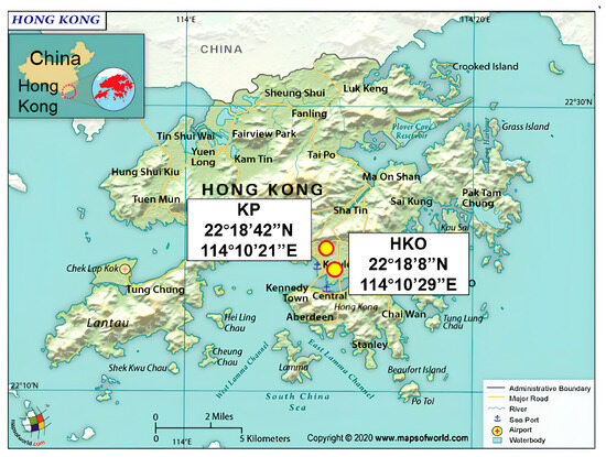
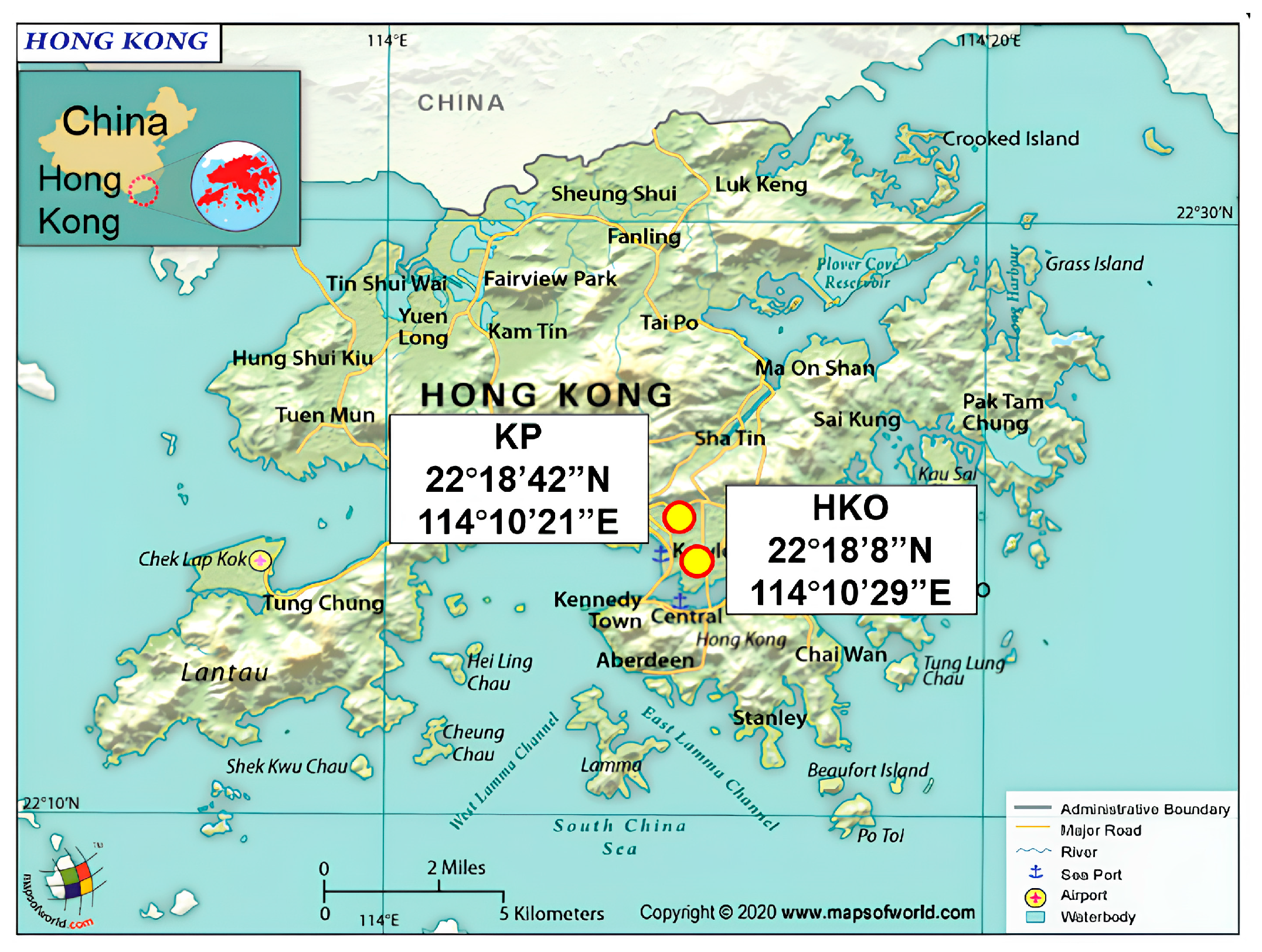
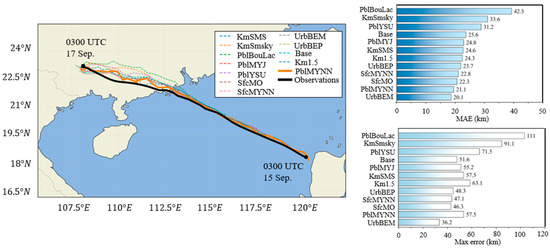
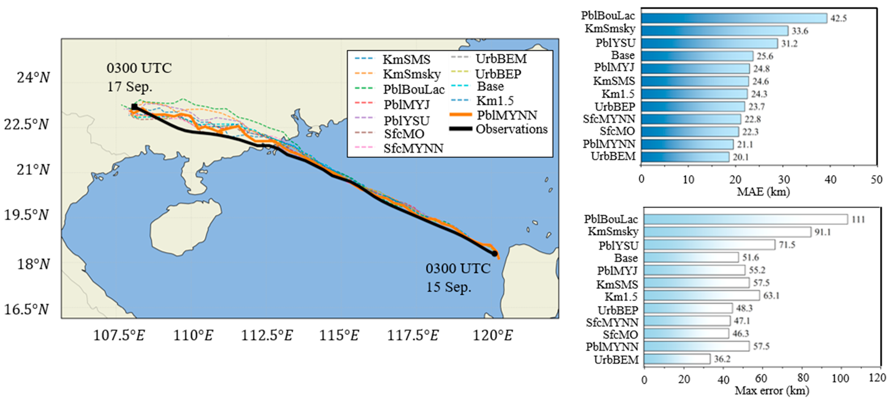
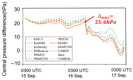
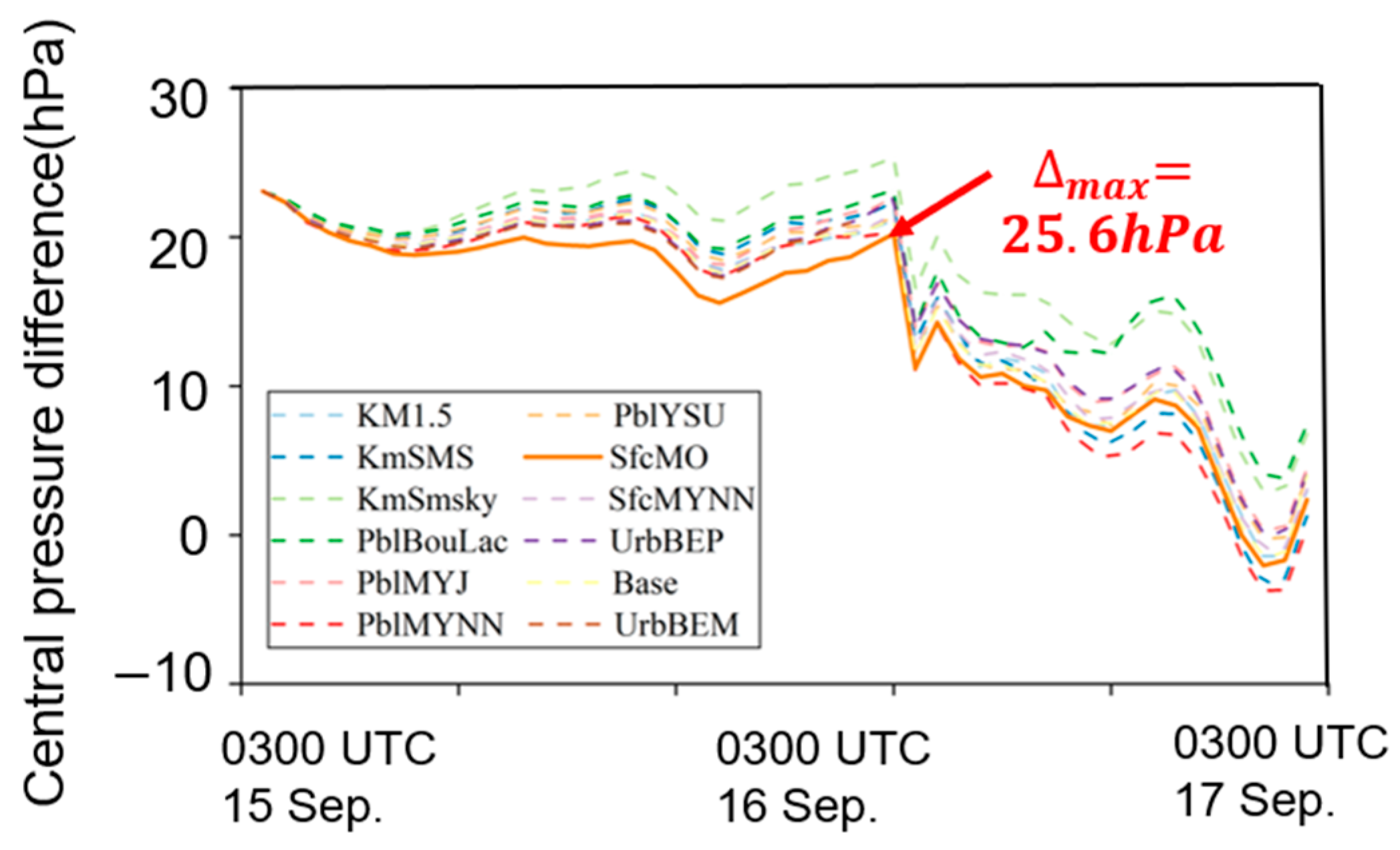
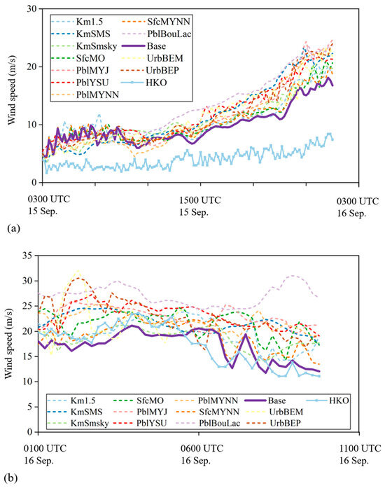
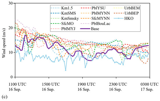
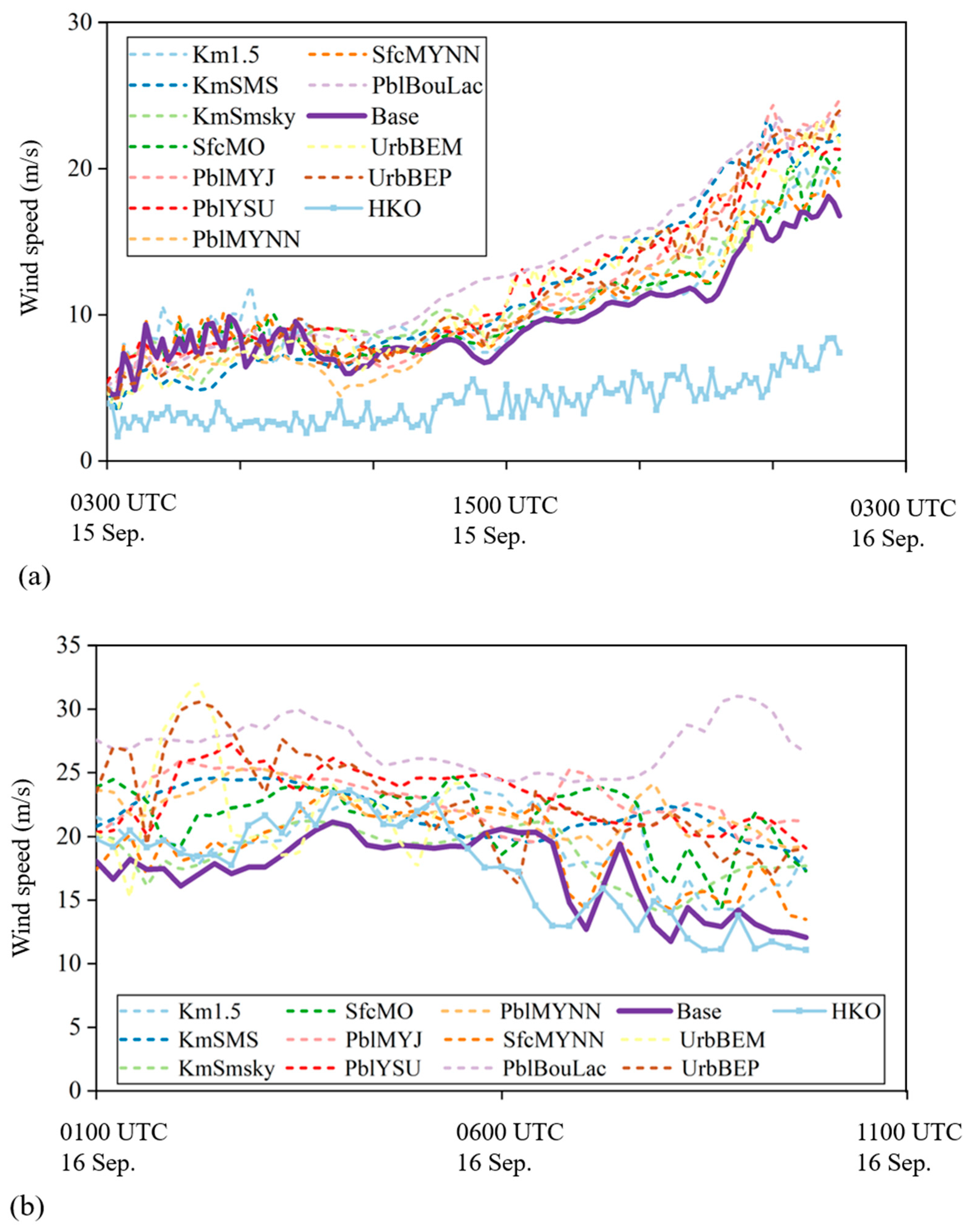
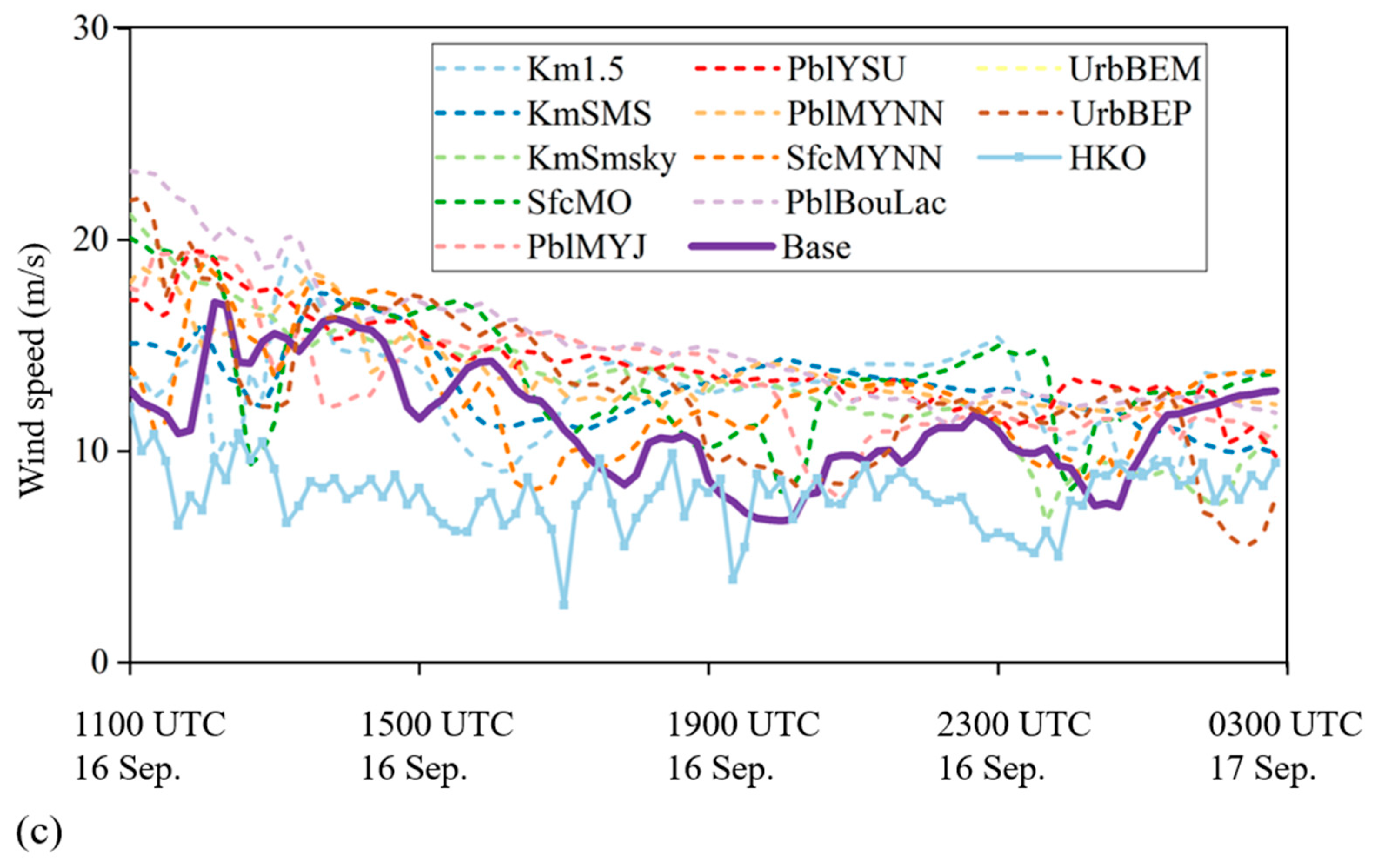
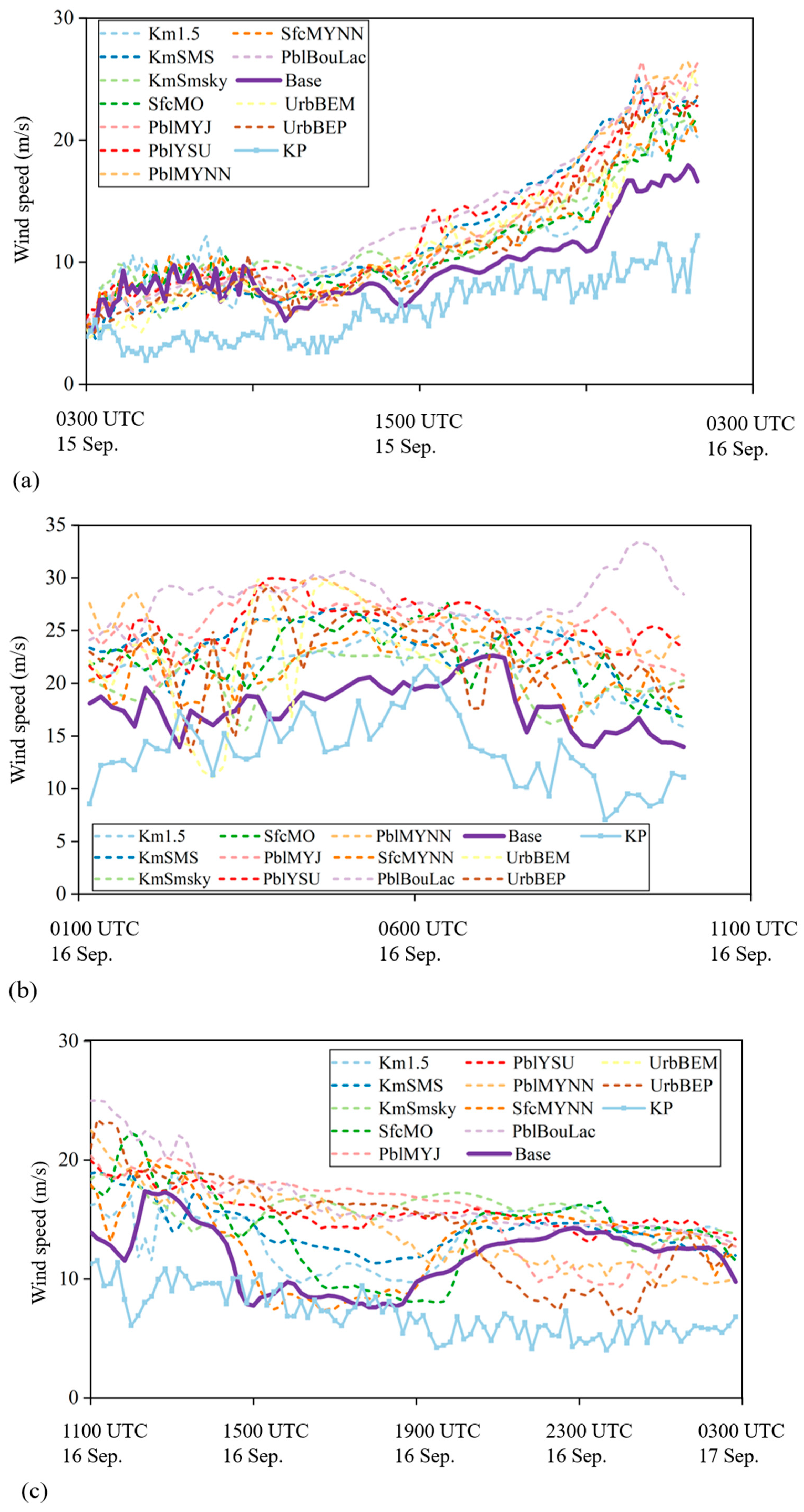
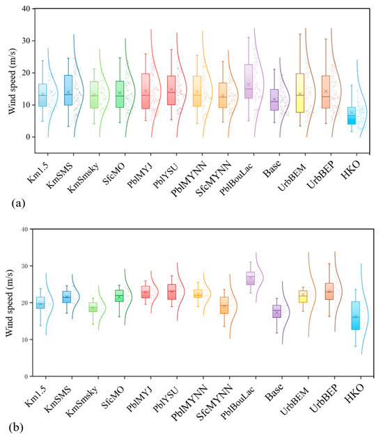
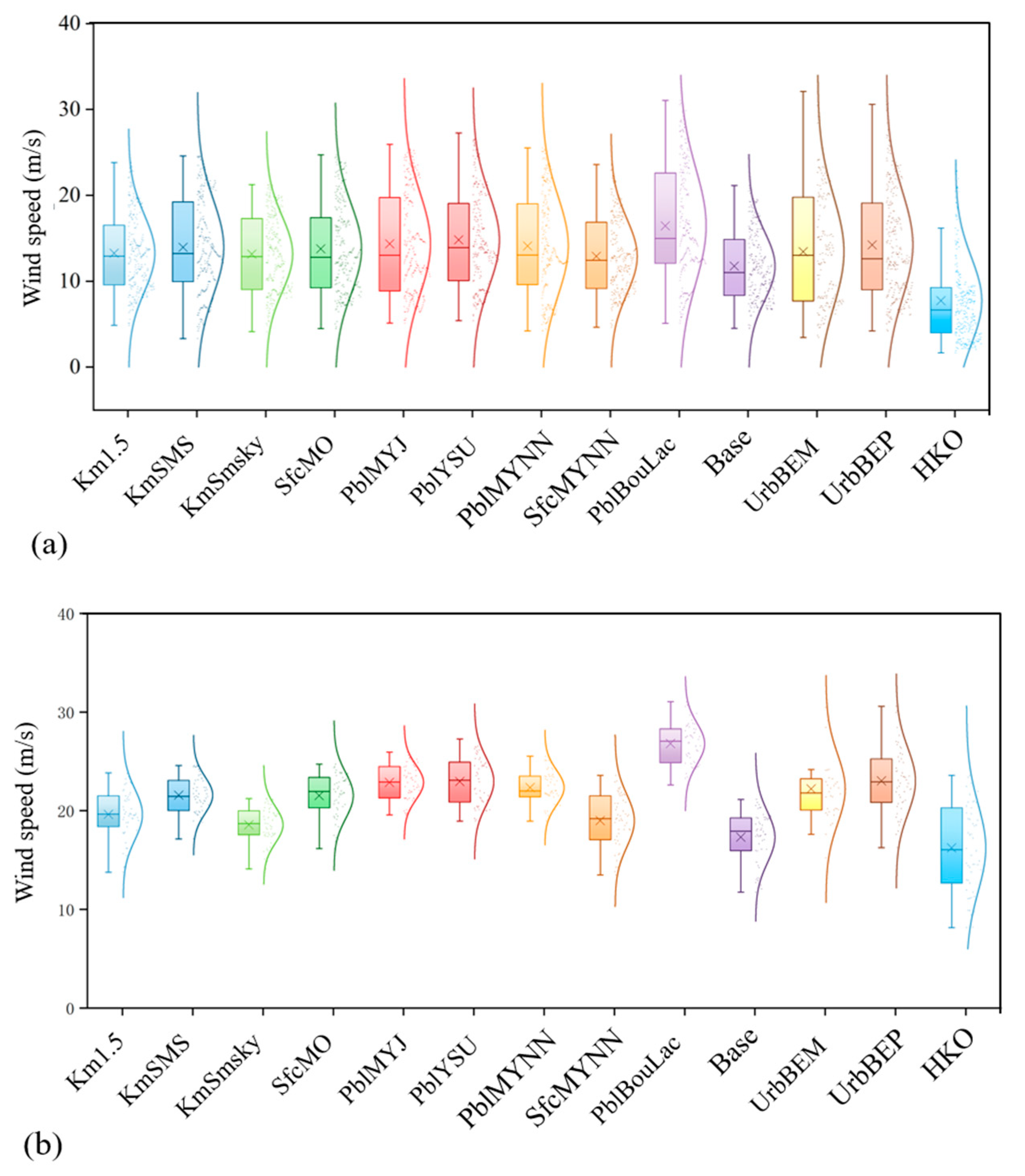
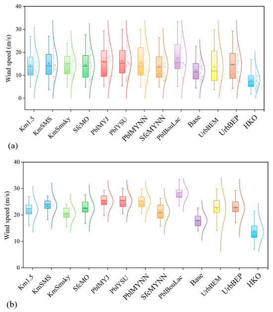
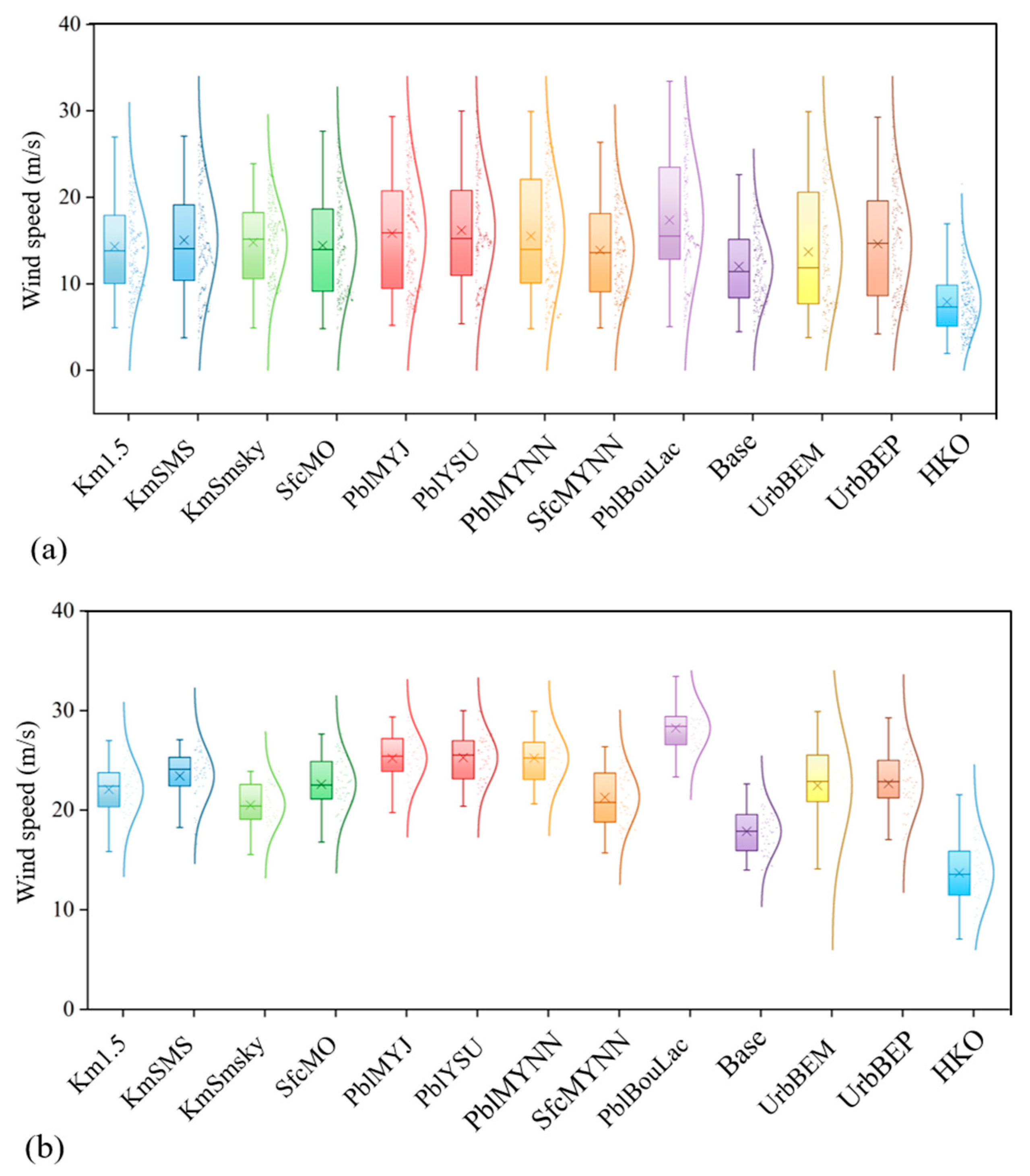
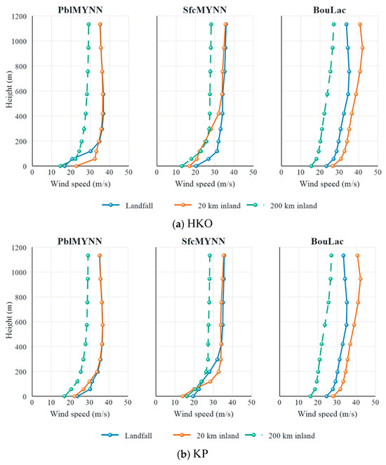
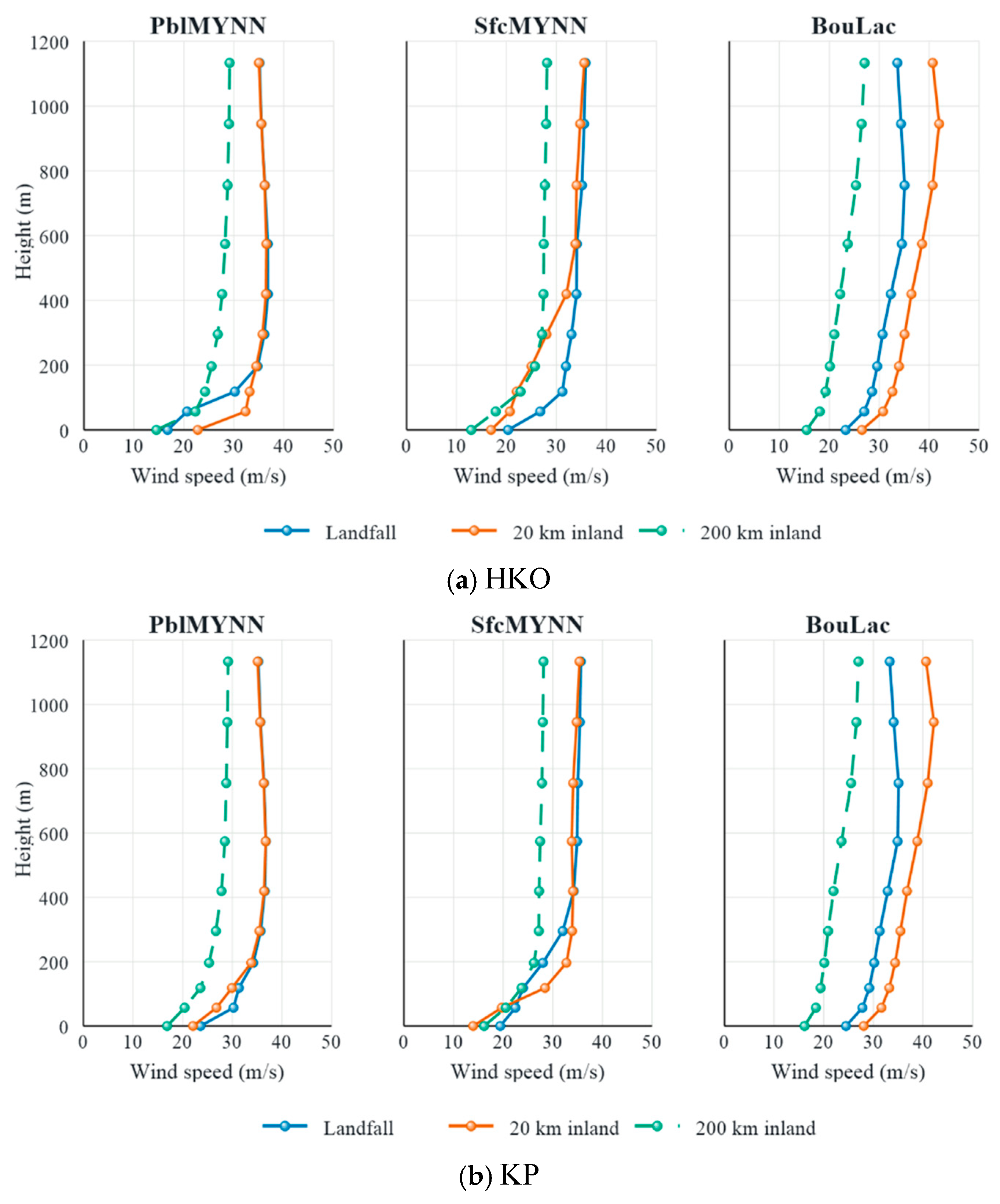
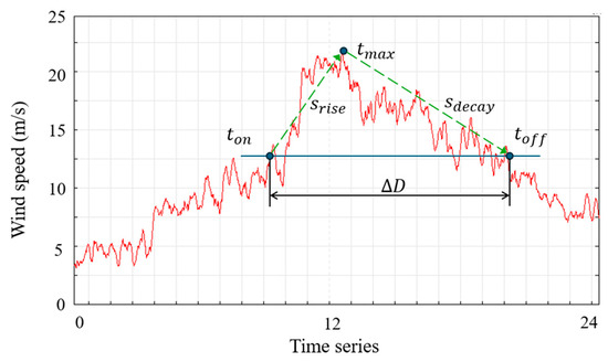
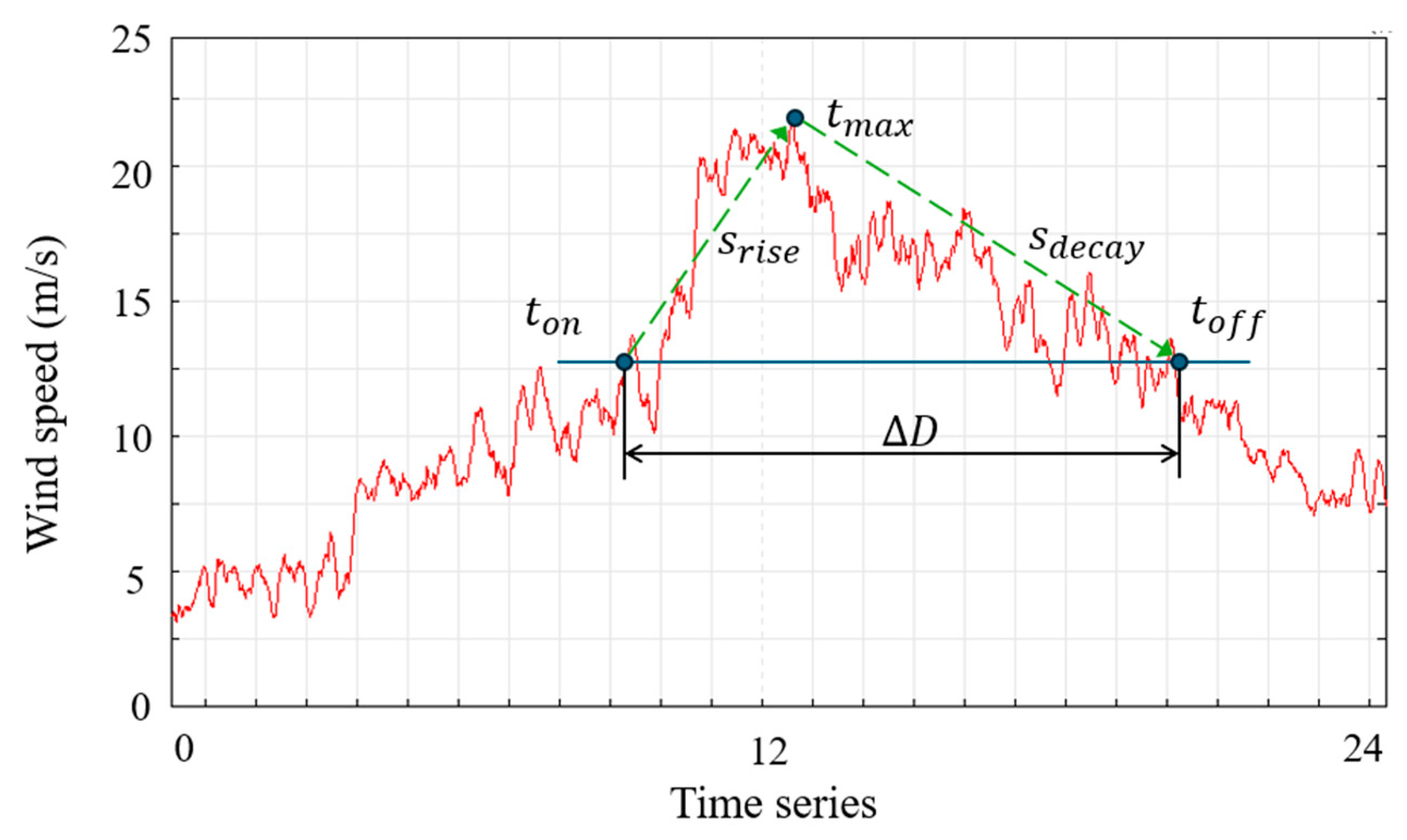

Disclaimer/Publisher’s Note: The statements, opinions and data contained in all publications are solely those of the individual author(s) and contributor(s) and not of MDPI and/or the editor(s). MDPI and/or the editor(s) disclaim responsibility for any injury to people or property resulting from any ideas, methods, instructions or products referred to in the content. |
© 2026 by the authors. Licensee MDPI, Basel, Switzerland. This article is an open access article distributed under the terms and conditions of the Creative Commons Attribution (CC BY) license.