Nested Sampling for Detection and Localization of Sound Sources Using a Spherical Microphone Array ^†

Abstract

Since its inception in 2004, nested sampling has been used in acoustics applications. This work applies nested sampling within a Bayesian framework to the detection and localization of sound sources using a spherical microphone array. Beyond an existing work, this source localization task relies on spherical harmonics to establish parametric models that distinguish the background sound environment from the presence of sound sources. Upon a positive detection, the parametric models are also involved to estimate an unknown number of potentially multiple sound sources. For the purpose of source detection, a no-source scenario needs to be considered in addition to the presence of at least one sound source. Specifically, the spherical microphone array senses the sound environment. The acoustic data are analyzed via spherical Fourier transforms using a Bayesian model comparison of two different models accounting for the absence and presence of sound sources for the source detection. Upon a positive detection, potentially multiple source models are involved to analyze direction of arrivals (DoAs) using Bayesian model selection and parameter estimation for the sound source enumeration and localization. These are two levels (enumeration and localization) of inferential estimations necessary to correctly localize potentially multiple sound sources. This paper discusses an efficient implementation of the nested sampling algorithm applied to the sound source detection and localization within the Bayesian framework.

1. Introduction

Nested sampling (NS) was introduced by Skilling [1] as a numerical method for efficient Bayesian calculations. Soon afterward, this method was applied to acoustics problems [2], where Jasa and Xiang explored using Lebesgue integral as the mathematical foundation of the NS algorithm. Since then, that effort has resulted in a series of publications in acoustic applications [3,4,5]. This paper showcases that the NS algorithm has recently been applied in sound source detection and localization within a Bayesian framework. To detect and localize sound sources, the sound environment is sensed by a spherical microphone array whose signals are processed using a spherical Fourier transform. Spherical harmonics are exploited to process the acoustic data and to formulate the signal models. This paper emphasizes that source detection represents a model comparison problem, source enumeration represents a model selection problem, and source localization represents a parameter estimation problem, all of which can be efficiently accomplished within the Bayesian framework using the NS algorithm.

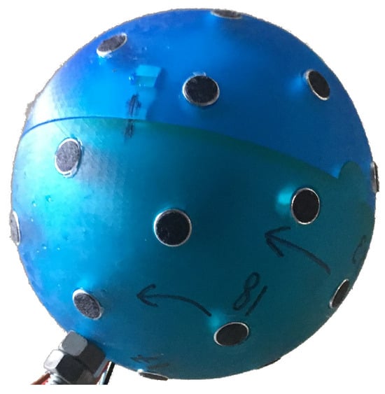
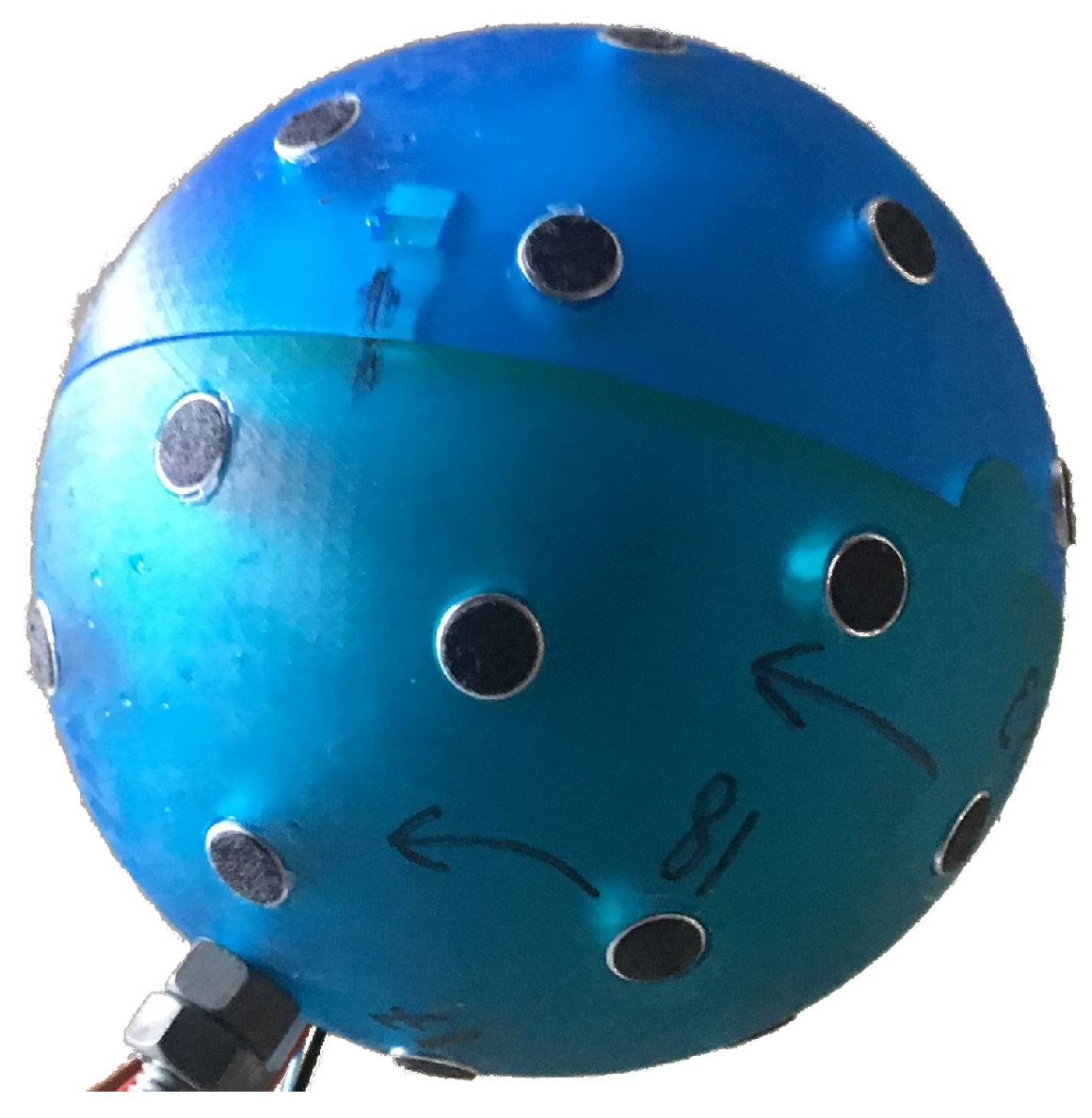
This paper presents a further development from the previous work [6] in that a background model for a no-source scenario needs to established. The source detection problem is critically based on the model comparison between the no-source and one-source models. Special attention is given to the spherical harmonics when dealing with the background model and is separately dealt with in Section 2.2. In addition to these model improvements, higher-order (fourth) spherical components have been achieved due to the further development of a 32-channel microphone array as illustrated in Figure 1.

Figure 1. Spherical microphone array of radius $a=3.5$ cm. Altogether, 32 microphones are nearly uniformly flush-mounted over the rigid spherical surface.

2. Spherical Microphone Data and Models

This section briefly introduces the data processing and the prediction models used for the sound source detection, enumeration, and direction of arrival estimations.

2.1. Microphone Array Data

When Q microphones are arranged flush on a rigid sphere of radius a nearly equidistantly, the sound pressure signals ${\underline{P}}_{mic}$ are processed by

$$D(\Theta )=\frac{4\pi }{Q}\sum _{n=0}^N\sum _{m=-n}^n\frac{{\underline{Y}}_n^m(\Theta )}{B\left(ka\right)}\sum _{q=1}^Q{\underline{P}}_{\mathrm{mic}}\left({\Theta }_q\right){\underline{Y}}_n^m{\left({\Theta }_q\right)}^{*},$$

(1)

with the third sum over $q=1,\dots ,Q$ being a spherical Fourier transform of Q microphone signals ${\underline{P}}_{\mathrm{mic}}\left({\Theta }_q\right)$ at angular positions ${\Theta }_q$, and symbol ∗ standing for a complex conjugate. Function $B\left(ka\right)$ is a modal strength of the rigid sphere of radius a,

$$B\left(ka\right)=\mathrm{j}k\left[j_n\left(ka\right)-\frac{j_n^{\prime }\left(ka\right)}{h_n^{\prime }\left(ka\right)}{h}_n\left(ka\right)\right],$$

(2)

where $\mathrm{j}=\sqrt{-1}$, $k=\omega /\mathrm{c}$ is the propagation coefficient of sound waves. Functions $j_n(·)$ and $h_n(·)$ are spherical Bessel and Hankel functions, and $j_n^{\prime }(·)$ and $h_n^{\prime }(·)$ are their derivatives, respectively. $\Theta =\{\theta ,\varphi \}$, collectively represents elevation and azimuth angles, while ${\Theta }_q$ specifies Q microphone locations flush-mounted on the spherical surface of the rigid sphere of radius a. Figure 1 shows a spherical microphone array of $Q=32$ channels developed for this research. The spherical array is built upon a rigid sphere of radius $a=3.5$ cm. In the following, we denote $\mathbf{D}=\left\{D\right(\Theta \left)\right\}$ as a two-dimensional matrix (vectors) representing the experimental data in the context of Bayesian inferential inversion.

2.2. Prediction Models

In Equation (1), ${\underline{Y}}_n^m(\Theta )$ is so-called spherical harmonics of order n and degree m, it is orthonormal and complete in a sense, and

$$g({\Theta }_s,\Theta )=2\sqrt{\pi }\sum _{n=0}^N\sum _{m=-n}^n{\underline{Y}}_n^m{\left({\Theta }_s\right)}^{*}{\underline{Y}}_n^m(\Theta )\to \delta (cos\theta -cos{\theta }_s)\delta (\varphi -{\varphi }_s),$$

(3)

when $N\to \infty$. ${\Theta }_s$ is the source angle in the form of the direction of arrival (DoA). $\delta (·)$ represents the Kronecker delta function. Using Equation (3), we establish a predictive model of spherical beamforming as

$$M_S({\Theta }_S,\Theta )=\sum _{s=1}^S\frac{A_s{g}^2({\Theta }_s,\Theta )}{max\left[g^2({\Theta }_s,\Theta )\right]},$$

(4)

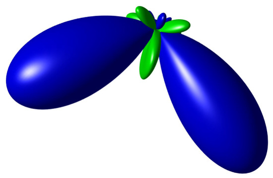
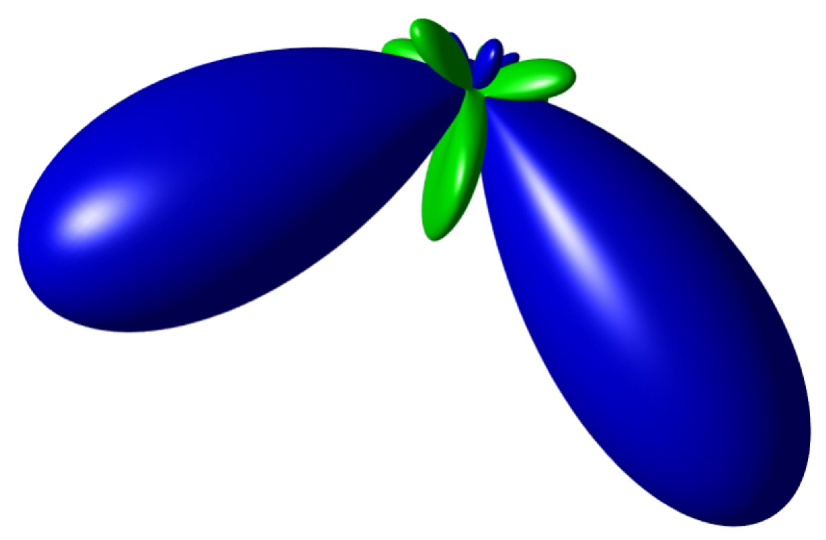
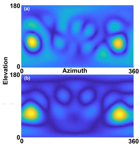
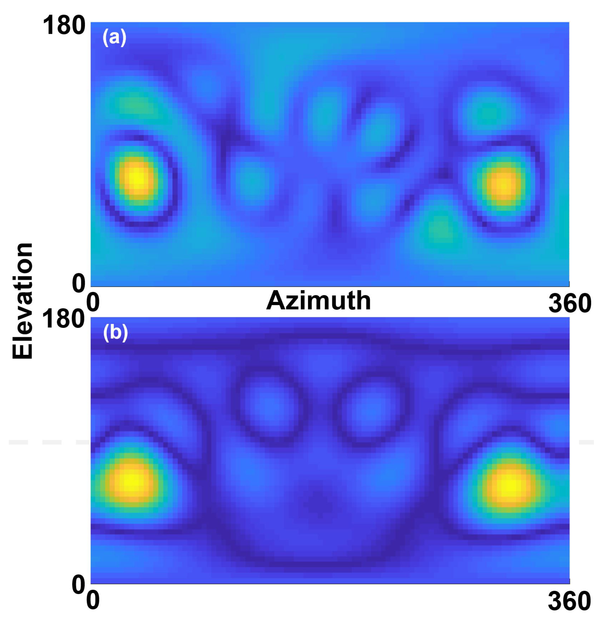
where $A_s$ counts for different source energy strengths of individual sound sources. Note that ${\Theta }_S=\{A_1,A_2,\dots ,A_S,{\Theta }_1,{\Theta }_2,\dots ,{\Theta }_S\}$ collectively denotes both strength vector $A_S$ and angular directions (vectors) of S sound sources, and each angular vector contains one pair of elevation and azimuth angles ${\Theta }_s=\{{\theta }_s,{\varphi }_s\}$. Variable $\Theta$ represents the angular range for possible sound sources to be localized. For $S\ge 1$, the kernel function $g({\Theta }_s,\Theta )$ in Equation (3) is processed for the upper order ${(N+1)}^2\le Q$. This means that the integer-valued order N of the spherical harmonics is limited by the number of microphone channels instead of infinity. Figure 2 illustrates a superposition of two simultaneous sources of equal amplitudes predicted by the model kernel in Equation (3) for $N=4$ before squaring the operation to build source energy. The finite upper order N is responsible for the width of lobes rather than middle-form ones. Figure 3a illustrates the spherical microphone data for the presence of two simultaneous sound sources, processed using Equations (1) and (2), while Figure 3b illustrates the predicted map of the two simultaneous sound sources using the model in Equation (4). The angular range is evaluated over $\Theta =\{0\le \theta \le {180}^{\circ };0\le \varphi \le {360}^{\circ }\}$.

Figure 2. Beamforming superposition of two sound sources using a spherical order $N=4$.

Figure 3. Comparison between the experimental data (a) processed according to Equation (1) with the prediction model (b) in Equation (4) of two sound sources using a spherical order $N=4$.

When processing the microphone array data, there is no prior knowledge about the incoming sound field either with the presence or absence of sound sources. It does not make sense to pursue direction of arrival analysis if no sound sources are present in the incoming microphone signals. For the model-based Bayesian detection, we need to establish a background model. Special attention has to be given to the spherical harmonics processing in this case. Specifically, $M_0$ represents the no-source model for $S=0$. In this case, the kernel function $g({\Theta }_0,\Theta )$ in Equation (3) is only calculated for $N=0$, namely the zero-order of the spherical harmonics.

$$M_0(\Theta )=\frac{A_0{g}^2(\Theta )}{max\left[g^2(\Theta )\right]},$$

(5)

where the direction of ‘no-source’ ${\Theta }_0$ is irrelevant over the angular range $\Theta$. For notation purpose, we collectively denote ${\mathbf{M}}_{\mathrm{S}}=\{M_0,M_1,\dots ,M_S\}$ as being the prediction models for the directional of arrival analysis, while we denote ${\mathbf{M}}_{\mathrm{D}}=\{M_0,M_1\}$ for the sound source detection, a small subset of ${\mathbf{M}}_{\mathrm{S}}$.

3. Bayesian Calculations

Given the data $\mathbf{D}$ as formulated in Section 2.1 and the prediction models $M_S\left({\Theta }_S\right)$ in Section 2.2, this work relies on Bayes theorem:

$$\begin{array}{ccccccc}p\left({\Theta }_S\right|\mathbf{D},M_S)& \times & \mathcal{Z}& =& \mathcal{L}\left({\Theta }_S\right)& \times & \Pi \left({\Theta }_S\right),\\ \mathrm{posterior}& \times & \mathrm{evidence}& =& \mathrm{likelihood}& \times & \mathrm{prior},\end{array}$$

(6)

with $\Pi \left({\Theta }_S\right)=p\left({\Theta }_S\right|M_S)$ being the prior probability and $\mathcal{L}\left({\Theta }_S\right)=p\left(\mathbf{D}\right|{\Theta }_S,M_S)$ being the likelihood function. The prior and the likelihood are both prior probabilistic in nature and need to be assigned a priori. This work applies the principle of maximum entropy (MaxEnt), which leads to a uniform prior and a Student-T distribution for the likelihood (see Ref. [6] for details). The evidence $\mathcal{Z}$ in Equation (6) plays a central role for the source detection and source enumeration problems and is determined by

$$\mathcal{Z}={\int }_{{\Theta }_S}\mathcal{L}\left({\Theta }_S\right)\Pi \left({\Theta }_S\right)\mathrm{d}{\Theta }_S={\int }_0^1\mathcal{L}\left(\mu \right)\mathrm{d}\mu ,$$

(7)

where

$$\mu \left({\mathcal{L}}_{ϵ}\right)={\int }_{\mathcal{L}\left({\Theta }_S\right)>{\mathcal{L}}_{ϵ}}\Pi \left({\Theta }_S\right)\mathrm{d}{\Theta }_S$$

(8)

is the prior mass with $\mathcal{L}\left(\mu \left({\mathcal{L}}_{ϵ}\right)\right)={\mathcal{L}}_{ϵ}$, and $0\le {\mathcal{L}}_{ϵ}\le {\mathcal{L}}_{\max }$ as derived by Skilling [7]. The NS algorithm generates a monotonically increasing partition of the likelihood range $[0,{\mathcal{L}}_{\max }]$

$$0<{\mathcal{L}}_0<{\mathcal{L}}_1<\cdots <{\mathcal{L}}_{T-1}<{\mathcal{L}}_T<{\mathcal{L}}_{\max },$$

(9)

via constrained sampling such that ${\mathcal{L}}_t$ with $t\in \{0,1,\cdots ,T\}$ is sampled from the domain $({\Theta }_S:\mathcal{L}\left({\Theta }_S\right)>{\mathcal{L}}_{t-1})$. Observe that as ${\mathcal{L}}_{ϵ}$ increases from 0 to ${\mathcal{L}}_{\max }$, ${\mu }_{ϵ}$ decreases from 1 to 0, where ${\mu }_{ϵ}=\mu \left({\mathcal{L}}_{ϵ}\right)$ and the partition of Equation (9) generates the monotonically decreasing sequence

$$1>{\mu }_0>{\mu }_1>\cdots >{\mu }_{T-1}>{\mu }_T>0.$$

(10)

Using the sequences in Equations (9) and (10), the one-dimensional integration on the far-right-hand side of Equation (7) is well approximated by

$$Z\leftarrow \sum _{t=0}^T{\mathcal{L}}_t\Delta {\mu }_t,$$

(11)

with

$$\Delta {\mu }_t={\mu }_t-{\mu }_{t+1},\mathrm{or}\Delta {\mu }_t={\mu }_{t-1}-{\mu }_t.$$

(12)

Skilling [7] pointed out that the constrained prior mass is a statistical quantity and follows a shrinkage of

$${\mu }_t\approx {\mathrm{e}}^{-t/P},$$

(13)

after t iterations, with P being an integer number for initializing random samples. A detailed proof of this result was given using order statistics in Appendix B of Jasa and Xiang [3].

NS was shown by Jasa and Xiang [3] to be a numerical implementation of Lebesgue integration, where Equation (11) represents the sum of weighted integrands of simple functions that are generated by partitioning the range rather than the domain of the function. An early account of this connection of the NS algorithm to Lebesgue integration can also be found in Jasa and Xiang [2], published in the Proceedings of the 25th International Workshop on Bayesian Inference and Maximum Entropy Methods in Science and Engineering (MaxEnt 2005).

4. Sound Source Detection, Enumeration, and Localization

The above described calculation is implemented for $P=500$ [in Equation (13)], the initial population with uniformly distributed prior ranges of all pending parameters, including sound source strength $A_s$, the elevation ${\theta }_S$, and azimuth angles ${\varphi }_S$. For potentially simultaneous sound sources up to four ($S\le 4)$, the parameter space is of dimensions up to $3\times S$. The NS is applied to estimating Bayes factors for model order from 1 to 4 via evidence. It is used to rank a potential model accounting for an unknown number of simultaneous sound sources, in a so-called sound source enumeration process. This process has also been described previously in Xiang and Landschoot [6], followed by a DoA analysis based on the selected model $M_S$ that is carried out by Bayesian parameter estimation. When examining this effort critically, the authors recognize that the source enumeration, even if representing a higher level of inference via Bayesian model selection, would still be incomplete if the machine sensory modality, such as in this application of a spherical microphone array, is not notified that the absence of sound sources often represents predominant portions of the sound environment in practical scenarios. It will only make sense to pursue sound source enumeration and DoA analysis if any sound source is ever detected.

The sound source detection is carried out in the scope of this current work using Bayesian model comparison. The prediction models ${\mathbf{M}}_{\mathrm{D}}=\{M_0,M_1\}$ solely involve two models, $M_0$ in Equation (5) and $M_1$ in Equation (4) for $S=1$. Note that Equation (5) is separately described because the $g^2({\Theta }_0,\Theta )$ needs special attention, in which the spherical order is set to $N=0$, while, for $M_S$ for $S\ge 1$, the spherical order $N=4$ due to the 32-channel spherical microphone array used for this work.

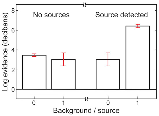
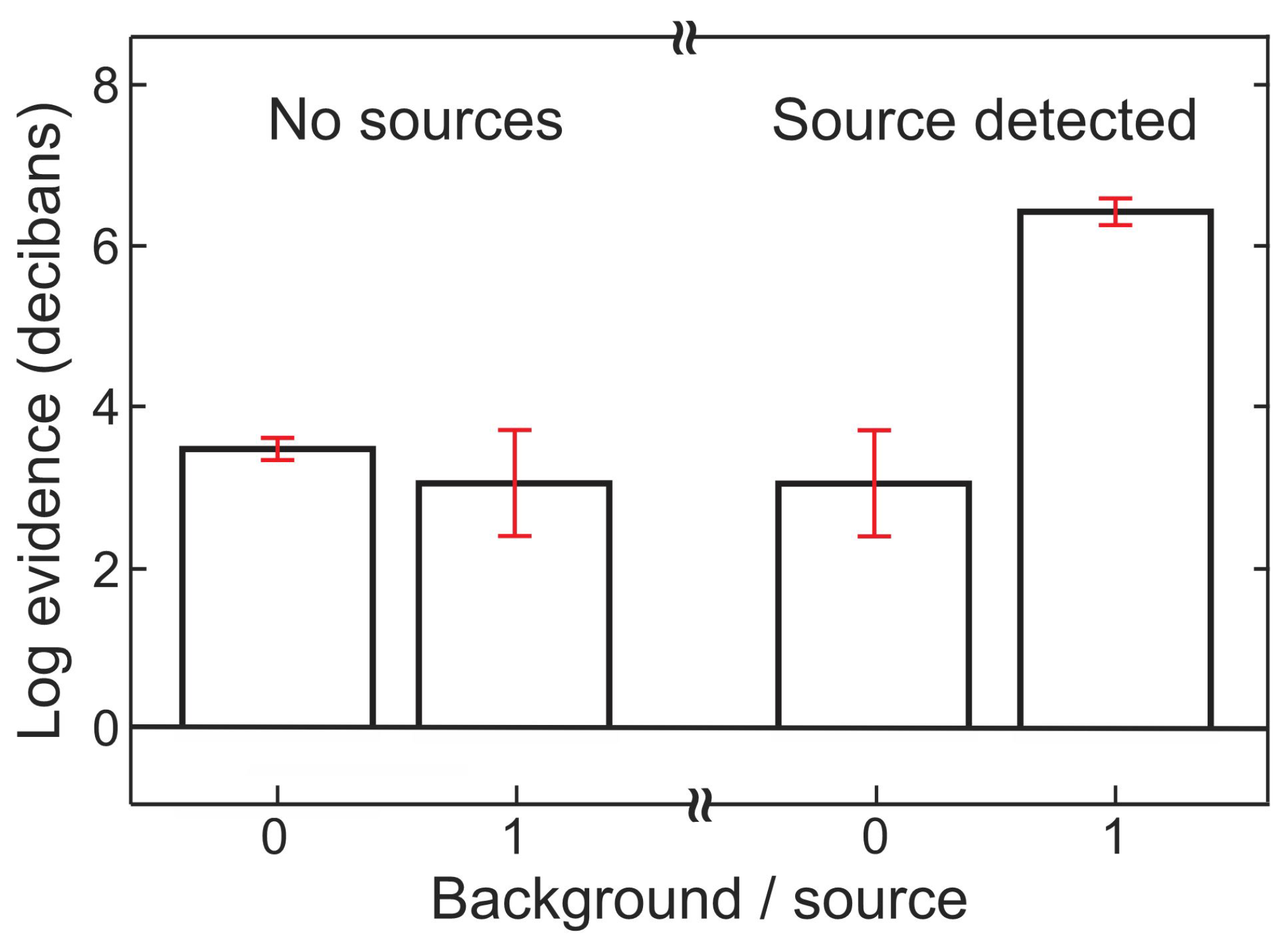
For the source detection, Bayesian evidence is estimated using the NS based on the ‘no-source’ model $M_0$ against the ‘one-source’ model $M_1$. Specifically, for $M_0$-based sampling, there is still one pending parameter $A_0$ to sample. Figure 4 (left) shows an experimental investigation when the microphone array data contain no sources but noisy background signals. The evidence estimation using the NS demonstrates insignificant differences to that of $M_1$, indicating that the source detection is negative. Figure 4 (right) shows that if the microphone array data contain sound sources, yet an unknown number, the evidence estimation clearly shows significant differences in comparison with those of ’no-sources’. The source detection is positive.

Figure 4. Sound source detection based on Bayesian model comparison. Bayesian evidence is estimated using both ’no-source’ model $M_0$ and one-source model $M_1$. The evidence is expressed in unit [decibans] in honor of Thomas Bayes [8].

Upon a positive detection of sound sources, a further process involves Bayesian model selection. A set of sound source models from $M_0$ to $M_4$ is involved for estimating Bayes factors:

$$B_{i,i-1}=10lg\left(\frac{{\mathcal{Z}}_i}{{\mathcal{Z}}_{i-1}}\right),\left[\mathrm{decibans}\right]$$

(14)

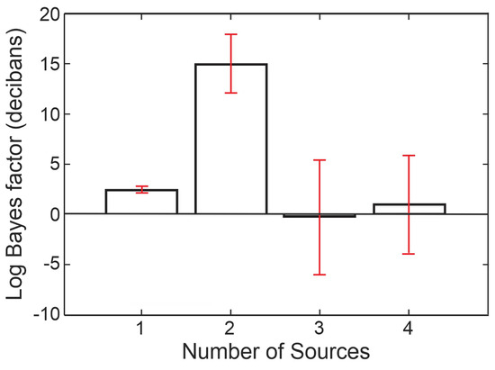
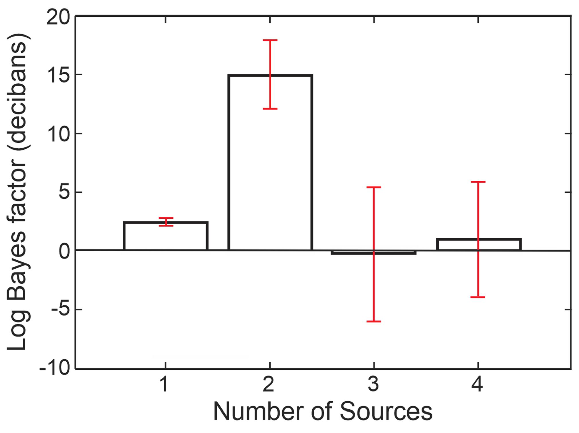
for $i=1,2,\dots 4$. Figure 5 illustrates one set of Bayes factor estimations. In this work, the evidence and Bayes factors are calculated in units [decibans] denoting 10 times logarithm base 10 $[10lg]$ in honor of Thomas Bayes [8]. In this case, the source enumeration using Bayesian model selection suggests that two sources are contained in the data. At this stage, the interest in specific DoA parameters is pushed into background. Upon the selection of a two-source model using the NS, the exploration samples during the iterative NS process also provide posterior samples for the model $M_2$ as a byproduct; they are readily available once the evidence ${\mathcal{Z}}_2$ for two sound sources is sufficiently explored. The posterior samples provide parameter estimates of two sound sources in terms of source strength $A_2$, and angular parameters ${\Theta }_2$. The data processed using Equation (1) and the model prediction according to the posterior estimates are compared in Figure 3.

Figure 5. The sound source enumeration based on Bayes factor estimation. The Bayes factors are expressed in unit [decibans] in honor of Thomas Bayes [8]. A two-source model is preferred by the Bayesian model selection. The evidence estimated using nested sampling also provides the posterior as a byproduct.

5. Concluding Remarks

From its introduction into Bayesian calculations, Skilling’s nested sampling [1] had an immediate impact on room-acoustic research [2], where an early account of the Lebesgue integral view on the nested sampling was first exposed in the MaxEnt Community in 2005. A thorough handling of its mathematical foundation of the Lebesgue integral was given at a later point [3]; ‘Interpreting nested sampling as a statistical approximation of a Lebesgue integral opens the possibility of a large body of existing research to be applied in the analysis and possible extension of the algorithm’. Over the past 15 years, a stream of applications using NS in acoustics science and engineering has emerged. Among others, this paper reports on an acoustic application of nested sampling using a spherical microphone array within the Bayesian framework.

References

- Skilling, J. Nested sampling. In Proceedings of the Bayesian Inference and Maximum Entropy Methods in Science and Engineering, AIP Conference Proceedings, Garching, Germany, 25–30 July 2004; Volume 735, pp. 395–405. [Google Scholar]
- Jasa, T.; Xiang, N. Using nested sampling in the analysis of multi-rate sound energy decay in acoustically coupled rooms. AIP Conf. Proc. 2005, 803, 189–196. [Google Scholar]
- Jasa, T.; Xiang, N. Nested sampling applied in Bayesian room-acoustics decay analysis. J. Acoust. Soc. Am. 2012, 132, 3251–3262. [Google Scholar] [CrossRef] [Scilit] [PubMed]
- Botts, J.M.; Escolano, J.; Xiang, N. Design of IIR Filters With Bayesian Model Selection and Parameter Estimation. IEEE Trans. ASLP 2013, 21, 669–674. [Google Scholar] [CrossRef] [Scilit]
- Fackler, C.J.; Xiang, N.; Horoshenkov, K.V. Bayesian acoustic analysis of multilayer porous media. J. Acoust. Soc. Am. 2018, 144, 3582–3592. [Google Scholar] [CrossRef] [Scilit] [PubMed]
- Xiang, N.; Landschoot, C. Bayesian Inference for Acoustic Direction of Arrival Analysis Using Spherical Harmonics. J. Entropy 2019, 21, 579. [Google Scholar] [CrossRef] [Scilit] [PubMed]
- Skilling, J. Nested sampling for general Bayesian computation. Bayesian Anal. 2006, 1, 833–859. [Google Scholar] [CrossRef] [Scilit]
- Jeffreys, H. Theory of Probability; Oxford University Press: Oxford, NY, USA, 1961; Reprinted by Clarendon Press, Oxford, NY, USA, 2003. [Google Scholar]
Disclaimer/Publisher’s Note: The statements, opinions and data contained in all publications are solely those of the individual author(s) and contributor(s) and not of MDPI and/or the editor(s). MDPI and/or the editor(s) disclaim responsibility for any injury to people or property resulting from any ideas, methods, instructions or products referred to in the content. |
© 2024 by the authors. Licensee MDPI, Basel, Switzerland. This article is an open access article distributed under the terms and conditions of the Creative Commons Attribution (CC BY) license (https://creativecommons.org/licenses/by/4.0/).