
Manifold-Based Geometric Exploration of Optimization Solutions †


Abstract
1. Introduction
2. Materials and Methods
| Algorithm 1 Calculate the encoding tree |
|
S ← set of all solutions L ← list of links sorted accordingly to the distance matrix tree ← buildNode(S, L) |
| Algorithm 2 Function buildNode(Solution Set S, Links List L) |
| if S has more than one solution then l ← first link of L (the best link) while S has no solution with l or S has no solution without l do Remove l from L l ← first link of L (the new best link) end while S1 ← the set of solutions of S with the link l S2 ← the set of solutions of S without the link l node ← new intermediate node with l Remove l from L node.leftChild ← buildNode(S1, L) node.rightChild ← buildNode(S2, L) return node else return new leaf node with the unique solution of S end if |
3. Results
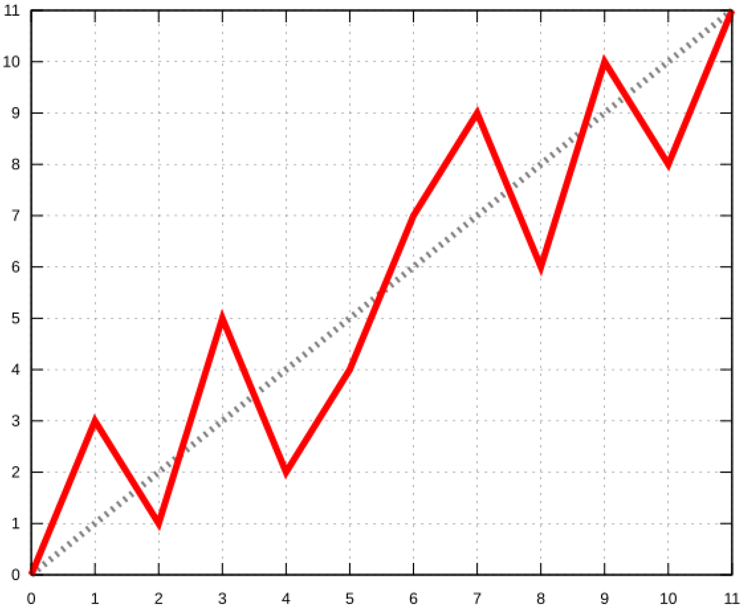
- The plots (a) and (b) represent a good resolution of the TSP. The optimum is the left most point, encoded with the value 0. The plots clearly show some branches of the encoding tree;
- The plots (c) and (d) display two examples where the optimum is not encoded with 0. It indicates that the tree incorrectly splits the solutions space at some point in the tree. Furthermore, the plot (d) shows that the optimum is not seen clearly in the first branch, which indicates that the wrong split is situated in the tree;
- The plots (e) and (f) show some examples where the encoding fails. The reason could be the low range of distances used for these TSPs. On the plot (e), the branches are difficult to see.
4. Discussion
- Build a portion of the encoding tree: the stopping criteria can be based on an upper bound of the optimum value [7];
- For each leaf node which has multiple solutions, choose the solution which uses the better links: the encoding is found by counting the solutions on the branches placed on the left side;
- Map a manifold of the objective value on the solutions space with the subset of solutions chosen:
- Find the minimum/minima of this manifold: as the function used is very simple, it should not be too difficult to differentiate and search for the stationary points;
- The optimum should be found on a neighbourhood of the minimum or one of the neighbourhoods of the minimum/minima if there are multiple local minimums on the solutions space.
Author Contributions
Funding
Institutional Review Board Statement
Informed Consent Statement
Data Availability Statement
Conflicts of Interest
References
- Hu, J.; Liu, X.; Wen, Z.W.; Yuan, Y.X. A Brief Introduction to Manifold Optimization. J. Oper. Res. Soc. China 2020, 8, 199–248. [Google Scholar] [CrossRef]
- Pop, P.C.; Cosma, O.; Sabo, C.; Sitar, C.P. A comprehensive survey on the generalized traveling salesman problem. Eur. J. Oper. Res. 2023, in press. [Google Scholar] [CrossRef]
- Bektas, T. The multiple traveling salesman problem: An overview of formulations and solution procedures. Omega 2006, 34, 209–219. [Google Scholar] [CrossRef]
- Miller, C.E.; Tucker, A.W.; Zemlin, R.A. Integer Programming Formulation of Traveling Salesman Problems. J. ACM 1960, 7, 326–329. [Google Scholar] [CrossRef]
- Dantzig, G.; Fulkerson, R.; Johnson, S. Solution of a Large-Scale Traveling-Salesman Problem. J. Oper. Res. Soc. Am. 1954, 2, 393–410. [Google Scholar] [CrossRef]
- Papadimitriou, C.H. The Euclidean travelling salesman problem is NP-complete. Theor. Comput. Sci. 1977, 4, 237–244. [Google Scholar] [CrossRef]
- Fischetti, M.; Salazar González, J.J.; Toth, P. A Branch-and-Cut Algorithm for the Symmetric Generalized Traveling Salesman Problem. Oper. Res. 1997, 45, 378–394. [Google Scholar] [CrossRef]


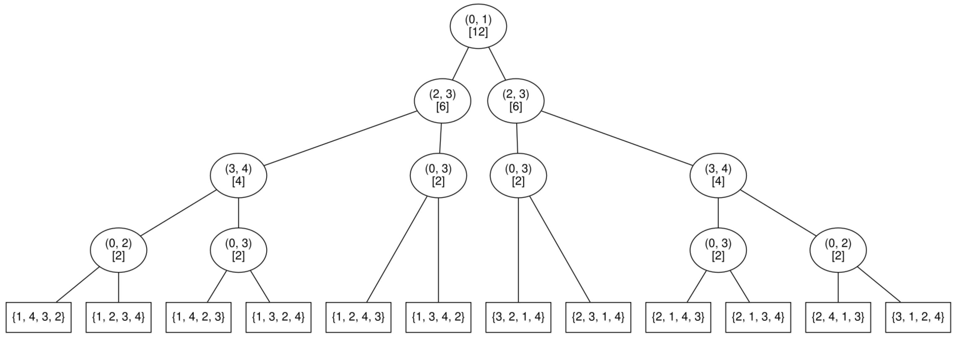
| Distance | Link |
|---|---|
| 8 | (0, 1) |
| 9 | (2, 3) |
| 15 | (3, 4) |
| 21 | (2, 4) |
| 37 | (0, 3) |
| 39 | (0, 2) |
| 45 | (1, 2) |
| 47 | (1, 3) |
| 49 | (1, 4) |
| 50 | (0, 4) |
| Encoding | Solution |
|---|---|
| 0 | {1, 4, 3, 2} |
| 1 | {1, 2, 3, 4} |
| 2 | {1, 4, 2, 3} |
| 3 | {1, 3, 2, 4} |
| 4 | {1, 2, 4, 3} |
| 5 | {1, 3, 4, 2} |
| 6 | {3, 2, 1, 4} |
| 7 | {2, 3, 1, 4} |
| 8 | {2, 1, 4, 3} |
| 9 | {2, 1, 3, 4} |
| 10 | {2, 4, 1, 3} |
| 11 | {3, 1, 2, 4} |
Disclaimer/Publisher’s Note: The statements, opinions and data contained in all publications are solely those of the individual author(s) and contributor(s) and not of MDPI and/or the editor(s). MDPI and/or the editor(s) disclaim responsibility for any injury to people or property resulting from any ideas, methods, instructions or products referred to in the content. |
© 2024 by the authors. Licensee MDPI, Basel, Switzerland. This article is an open access article distributed under the terms and conditions of the Creative Commons Attribution (CC BY) license (https://creativecommons.org/licenses/by/4.0/).
Share and Cite
Lebonvallet, G.; Hnaien, F.; Snoussi, H. Manifold-Based Geometric Exploration of Optimization Solutions. Phys. Sci. Forum 2023, 9, 25. https://doi.org/10.3390/psf2023009025
Lebonvallet G, Hnaien F, Snoussi H. Manifold-Based Geometric Exploration of Optimization Solutions. Physical Sciences Forum. 2023; 9(1):25. https://doi.org/10.3390/psf2023009025
Chicago/Turabian StyleLebonvallet, Guillaume, Faicel Hnaien, and Hichem Snoussi. 2023. "Manifold-Based Geometric Exploration of Optimization Solutions" Physical Sciences Forum 9, no. 1: 25. https://doi.org/10.3390/psf2023009025
APA StyleLebonvallet, G., Hnaien, F., & Snoussi, H. (2023). Manifold-Based Geometric Exploration of Optimization Solutions. Physical Sciences Forum, 9(1), 25. https://doi.org/10.3390/psf2023009025