


Abstract
Shannon’s channel-coding theorem permits arbitrarily reliable communication at rates below the channel capacity and rules it out above it. This paper asks the corresponding question of a system that acts irreversibly on what it infers: can its commitments still be undone? This matters because a decision that is not reviewed in time becomes permanent, right or wrong. The framework is called Recoverable Self-Coding (RSC). Candidate commitments arrive at rate , and one certifier checks them at rate ; both rates can be estimated from event counts. The framework proposes that irreversible action is admissible only while the margin is positive. The certifier is modelled as a single-server queue of capacity ratio , whose uncertified backlog is the mean number of commitments awaiting certification. An exact identity for holds at every CR below one; for fixed shapes with positive variability, , it grows as near , and three exact solutions agree with the simulation. Under the outcome model, the recoverable fraction of commitments falls from to as CR rises from to while accuracy stays at or above its floor , a separation that is derived rather than measured. Two limits follow: counting uncertainty sets the observation time needed to estimate the margin—centuries for the review board of the opening example—and the collapse belongs to pipelines that keep expired work. One application is offered as an untested hypothesis: artificial intelligence (AI) may raise the rate of proposed decisions faster than review capacity.
1. Introduction
Artificial intelligence (AI) is changing how consequential decisions are made. Candidate decisions have become cheap to produce, and fast and easy to scale, so institutions route more and more judgments through their most efficient decision step. That shift of tasks toward the cheaper route is documented for automation and labour more generally [1]. If those decisions arrive faster than the people and procedures that review them can check them, review falls behind. Approvals are still issued, but reviewers can lose the ability to trace a decision to its outcome and to reverse it before harm is done, and oversight becomes a formality. Section 8 states this sequence as a hypothesis, not as a measured fact. Safety science has described this failure for decades: systems drift toward the boundary of safe operation under pressure for efficiency [2], tightly coupled systems produce “normal accidents” [3], and layers of defence erode [4]. What the AI setting still lacks is a measurable quantity that indicates how close a system is to the point where its commitments can no longer be undone.
A small example shows the quantity proposed here. Suppose a review board can certify ten decisions a week while nine and a half arrive, so that the margin between the two rates is per week. Let the board behave as a single server with Poisson arrivals and exponential service times (the M/M/1 queue of Section 6), and let each decision need certification within a horizon of weeks. A decision is then certified in time with probability . Now consider a second board, identical except that arrivals are five percent higher. Its margin is per week and its about . The two numbers describe two stationary regimes, and the backlog of a board whose load rises takes time to settle into the second (Section 6.2). The quality of individual judgments is the same in both, yet the second board certifies few of its commitments before they become permanent. Distinguishing the two regimes by measurement is itself demanding, and Section 6.2 gives the observation span it takes. is only the probability of a first certification in time. Recoverability, defined in Section 5, also requires a corrective pass and is smaller still.
The quantity rests on an analogy with Shannon’s channel-coding theorem. A memoryless channel of capacity C permits arbitrarily reliable recovery of a message when the information rate R is below C, and rules it out when R is above C [5]. The claim of this paper is that a similar limit applies to systems that act irreversibly on what they infer. The claim is developed here for a system whose commitments pass through a single certifier. What fails near the limit in such a system is recoverability: whether a commitment can still be corrected or cancelled before the options it removes are gone (Section 5 gives the definition). The failure is measurable. As the system is driven toward its capacity, the accuracy of its decisions falls no lower than a floor, while the fraction of its commitments that remain recoverable falls toward zero. The floor is the accuracy of the decisions that were not certified in time (Section 7). In an institution, this separation would mean that decisions remain mostly correct while reviewers lose the ability to correct them in time.
The framework is called Recoverable Self-Coding (RSC), and the system it describes is a self-decoder. Candidate commitments arrive at rate , which the framework calls the induced flux, and the certifier can check them at rate , the integrative capacity. Their ratio is the capacity ratio, and the boundary plays the role that plays in Shannon’s theorem. The application hypothesis of Section 8 is that AI can increase the arrival rate of proposed decisions faster than the capacity to review them, bringing many workflows closer to . That change is not measured in this paper. The idea was introduced in the foundational preprint of this research programme [6], and an independent treatment has since reached the same thesis [7]. That treatment has no order parameter, that is, no measurable quantity that tracks the loss of recoverability, and no early-warning quantity. The present paper supplies the first and a candidate for the second.
The contributions are listed below so that what is new is distinguished from what is inherited.
- 1.
- Inherited. The mathematics is classical single-server queueing theory: the stability condition, the backlog law, the heavy-traffic asymptotics and the effective-bandwidth sojourn exponent are all standard results [8,9,10]. Proposition 1 collects the exact identity for the backlog, the Pollaczek–Khinchine form, the GI/M/1 sojourn law and the heavy-traffic limit, and proves them for the model in this paper.
- 2.
- New. The backlog of uncertified commitments is identified as the order parameter of recoverability, and operational definitions make , and the margin estimable from event counts alone (Section 3). Two limits on that proposal are then established. The counting precision of the margin degrades as the margin shrinks, so the observation span needed to resolve it grows as and, for the M/M/1 queue, is a fixed multiple of the relaxation time (Section 6.2). And the collapse of recoverability at is a property of a pipeline that keeps expired work: where expired work leaves the queue, the backlog stays bounded at every load (Section 6.2).
- 3.
- Distinguishing prediction. An ordinary congestion model bounds delay. This model gives separate measures to the opportunity for correction and to the quality of the decision: the fraction of commitments that remain correctable, and the accuracy of the decisions themselves. Within the model of Section 7 the first falls toward zero under load while the second keeps its floor, and that separation is derived rather than measured. What a logged workflow can test is whether the model describes it, and the tests are stated at the end of Section 7.
The claim is narrower than a theorem. Treating one certification as one channel use is a modelling step, not a derived result (Section 2). Reading the two rates as information rates is an analogy, and the results are those of a single-server model within the scope stated at each formula. No law is asserted for arbitrary systems.
The paper is organized as follows. Section 2 states the constraint and shows the model in a diagram, and Section 3 shows that its two parameters can be estimated from event data. Section 4 places the work in the literature. Section 5 defines recoverability and states the full constraint, Section 6 derives the law of the backlog, and Section 7 compares simulated backlogs with the exact results under a controlled statistical protocol and illustrates the analytical outcome model. Section 8 states one application, the loss of human agency under AI acceleration, as a hypothesis. Signatures in operational field data are left to future work [6].
2. Decoders and Their Constraints
From channel reliability to action recoverability. A self-decoder is any physical or informational system that turns uncertain observations into updates of its internal state and then into commitments, some of which are irreversible. Nothing in the definition depends on the substrate, so biological cognition and physiology, artificial computation, institutions and combined human–AI systems all qualify. Figure 1 shows the model: candidate commitments arrive one by one, and each must be certified, that is, checked against evidence, before it becomes irreversible. Those that have arrived and are not yet certified are counted by , whose mean is the backlog of Section 6. A commitment certified within the horizon is certified in time; one that misses is committed uncertified and is still served, because nothing leaves the queue early (Section 6.2 treats the alternative). It is recoverable if it was certified in time and a corrective pass, drawn independently from the law of the sojourn time and adding no load, would also finish within an option-loss window of length H. The queue is open: arrivals are exogenous and no output returns as load, so the closed loop of the companion paper [11] lies outside the figure, as does information retention (Section 5).
Figure 1.
The certification pipeline modelled in this paper: candidate commitments arrive at rate and wait for a single certifier of rate (top), and the two rates are estimated from an event log and combined with the law of the queue to give the backlog and the probability of certification in time (bottom), with an inset for the M/M/1 case at .
Over a finite decision horizon , the system is described by two rates. The induced informational flux is the arrival rate of candidate commitments that need certification, expressed in bits through the uncertainty quantum introduced below. It is measured through proxies such as queued decisions and uncertified candidate commitments, never through the raw data rate or a count of tokens per second. The effective integrative capacity is the rate at which candidate commitments can be certified. It is limited by throughput, buffering, the work of keeping the internal state consistent, and the latency of validation. The entity that certifies is the certifier; it is the single server of the queueing model of Section 6, and the review board above is one instance of it. A commitment awaiting certification is a candidate commitment, and one that has been certified or has missed its horizon is a commitment. Where every candidate commitment stays in the queue until it is certified, the framework proposes that recoverable operation requires
Equation (1) has the form of Shannon’s condition with a different decoded quantity. Shannon’s condition bounds how reliably a message is recovered, and Equation (1) is proposed as the condition under which an irreversible action can still be recovered in such a pipeline. In this sense, RSC states a rate–capacity condition for commitment. Both conditions concern feasibility, and neither limits speed. An encoder may emit symbols at an arbitrary rate, and a decision system may generate candidate commitments at an arbitrary rate. What the condition decides is whether the resulting stream can be decoded, or certified, as fast as it arrives.
What the constraint is built on. Let be the arrival rate of candidate commitments and the certification rate. To draw the analogy with information rates, assign to each commitment the same amount of uncertainty, an uncertainty quantum of bits that must be resolved to certify it. Multiplying by expresses both rates in bits per unit of time, and . The quantum cancels in , which is why counts are enough. Measured in channel uses instead of bits, with one channel use per certification, the two rates are and . Commitments with unequal quanta are handled by the load-weighted effective bandwidth [10,12,13].
The modelled system is allowed memory, since a person, an institution or a coupled human–AI system is not memoryless. Shannon’s memoryless channel supplies only the form of the limit, and what this paper actually uses is the stability boundary of a service process. That boundary, , exists for general stationary arrival and service processes. For the queue families of Proposition 1(e), which have fixed distribution shapes, finite second moments and positive variability, , the mean backlog grows as as CR approaches one (Section 6). Memorylessness is needed only for some of the explicit closed forms. When options are lost after a deadline , the allowed arrival rate must also meet a specified probability of deadline success. Effective-capacity methods estimate this relation under their traffic and service assumptions [13]. Section 6.2 gives exact deadline probabilities for the exponential-service queues used here.
The whole construction rests on one modelling step, which is to treat one certification as one channel use. This is a choice, not a theorem. Under it, the channel alphabet is the set of candidate commitments, and the coding operation is certification. The source uncertainty is the quantum to be resolved for each commitment. The capacity is the certification service rate, which is not a supremum of mutual information. The analogy would carry more weight if a converse held, that is, a proof that no certification discipline can sustain recoverable operation at . Loynes’ theorem [8] supplies that converse for stability: above the boundary, no stationary backlog distribution exists under any work-conserving discipline that keeps all incoming work. Loynes’ theorem gives no converse for the reading of the two rates as information rates. That reading therefore remains an analogy and is marked as one wherever it is used.
3. The Flux and the Capacity Are Measured Quantities
Because and are defined operationally as rates, both can be estimated from a stream of events without access to the internal model of the system. This section illustrates the estimation on physiological data, an example chosen because the data are openly available. The estimation has not been clinically validated. Physiological homeostasis is read as a biological self-decoder. A monitored variable that leaves its reference band is treated as a candidate commitment, so the rate of such crossings estimates the induced flux . The rate at which excursions return to the band estimates the integrative capacity .
The scope of the section is limited in two ways. The first limit is the meaning given to the events, which is a modelling choice. An out-of-range result can reflect the timing of measurements, a treatment or natural fluctuation, and need not be a commitment event at all. Validating the mapping against outcomes that represent restoration or failed recovery would take clinical expertise beyond the scope of this paper. The section therefore demonstrates that the rates can be measured and makes no claim of clinical validity. The second limit is that the restoration process is parallel, not serial, because several analytes can be out of range and return to range at the same time. The physiological data are therefore used only for the rates and and for their margin, quantities that are well defined for a parallel restoration process, which is an infinite-server process. In such a process, the stationary number of open excursions has mean , where is the duration of an excursion, and it stays finite at every load. The single-server law of Section 6 applies where certification passes through a finite shared bottleneck, as in the decision systems of Section 7 and Section 8, and is left aside for these data. The distinction matters, because the divergence needs such a bottleneck, and an infinite-server process has none.
The rates were first estimated on synthetic longitudinal health records [14], where both are well defined and non-degenerate across the population (Figure 2a). The margin follows directly for every unit (Figure 2b). The same computational procedure was then applied, with cohort-specific reference ranges, to real physiology. The data are the openly licensed demonstration subset of the Medical Information Mart for Intensive Care, version IV (MIMIC-IV) [15,16], read against its own per-assay reference bands. The procedure returns non-degenerate rates for 78 of its 100 patients, and Supplementary Table S1 gives the selection rules, the counts before and after exclusion, and the identity of each release. What the two cohorts establish is that the estimator runs on real event streams of two different kinds and returns finite rates for both. No comparison is drawn between them, for the reasons stated in the next paragraph.
Figure 2.
and measured from a longitudinal event stream of synthetic electronic health records [14], with homeostasis as the self-decoder and about 1900 units: (a) the distribution of the two measured rates, and (b) the two rates for each unit, with the line marked.
Why no contrast between the cohorts is drawn. The two shares of units below the reference line, of the synthetic units and of the critically ill patients, measure the observation scheme rather than a capacity property, and five analyses on the same pipeline establish it. As the estimator is coded, CR is the product of two factors: onsets per restoration, and the fraction of the observation span during which at least one analyte is out of range. The first factor exceeds one only when excursions are left open at the end of a record, and of the MIMIC-IV units and of the synthetic units do end on one, so the comparison is dominated by right-censoring. The median capacity ratio of the critically ill cohort, , is not significantly above one: a bootstrap over units gives . After the terminal censored excursions are excluded, onsets equal restorations, so the first factor is exactly one, CR equals the busy fraction of the observation span and cannot exceed one: the median falls to in the synthetic records and in MIMIC-IV, and both cohorts then read below the line. That is a property of the exclusion rule rather than a finding about either cohort. The two arms are also not measured on the same panel, since nine analytes resolve a usable reference band in the synthetic records against thirteen in MIMIC-IV, and the per-analyte capacity ratio varies by more than an order of magnitude within a cohort, so a single pooled value per unit averages over very different series. A censoring-aware duration estimator, such as Kaplan–Meier on excursion durations, is the method a future cohort study should use; at these censoring rates it would rest almost entirely on extrapolation, and it is left to that study. Figure 2 is therefore an illustration that the two rates are computable from an event log, which is what this section claims.
Because the restoration process is parallel, CR is here descriptive, and the line of Figure 2b is a reference marker, not the single-server stability boundary of Section 6; no region of that plane is a feasible set. With stationary arrivals and a finite mean excursion duration, an infinite-server model has no threshold in the capacity ratio at all. counts onsets per unit of observation span, and counts restorations per unit of time during which at least one excursion is open. CR therefore exceeds one only when counted excursions remain unresolved at the end of the series. Its value depends on the observation and censoring scheme, and no clinical or causal reading is drawn from it here. Supplementary Table S1 records the analysis details: the analyte panel, the eligibility and exclusion rules, the event definition, the censoring rules, and the dependence between events. The estimator also leaves the differences between the two observation processes in place. Sampling in intensive care is more frequent and is triggered by illness, the synthetic records are sampled on a different schedule, and CR may change with either. Both pipelines report rates per year, but the cohorts are observed over very different spans (days in intensive care, years in the synthetic records) and are sampled differently. Their absolute rates are therefore not compared. Matched-cadence analysis, sensitivity to downsampling, a pre-specified analysis plan and a receiver operating characteristic (ROC) analysis of detection remain future work; the censoring sensitivity, the per-analyte results and the bootstrap interval for the median capacity ratio are reported above.
4. Relation to Existing Work
Equation (1) draws on several established fields. The mechanism is familiar, and the contribution of this paper is to make it operational. Classical decision frameworks include expected utility and optimal control, risk management [17], real options [18], robust and safe-set methods [19,20] and AI alignment [21]. They address decision quality, risk and safety, and real options also address the cost of irreversible commitment. The present construction adds a different constraint: the certifier is congested, and the time available for correction is finite. The safety-science tradition [2,3,4], recently restated for AI [7], describes this failure qualitatively and gives no measure of it. The systems literature documents the same family of failures at engineering scale. Metastable failures in distributed systems are degraded states that persist after the trigger has been removed [22].
Within this research programme, the foundational preprint [6] introduces the idea and the estimator programme at length. The present paper adds a compact information-theoretic statement, a demonstration of measurability with its scope limits (Section 3), the derivation of the backlog law (Section 6), and the controlled ordering of accuracy and recoverability (Section 7). The companion physics paper [11] treats the closed-loop problem, in which uncertified output is consumed again as load and the transition becomes first-order, with hysteresis. Here, the queue is open, and the approach to the boundary is continuous (Figure 1). The independent treatment of [7] reaches the agency thesis without an order parameter.
Five neighbouring frameworks measure quantities close to the two described in this paper. Queues with deadlines and impatient customers study the mechanism of Section 6 directly: work that must be served before a deadline, and work that leaves when it waits too long. Barrer’s constant-deadline queue [23] and the general single-server treatment [24] supply the stationary laws used in Section 6.2, the many-server case with general patience is [25], and the earliest-deadline-first discipline has a heavy-traffic theory [26]. That literature computes the fraction of work that misses its deadline, and stops there. Age of information measures the staleness of what a monitor knows as the time since its last update, and optimizes update policies against it [27,28]; it is a freshness measure for information rather than an admissibility condition for action. Queueing models of human supervisory control treat an operator as a server and predict capacity from utilization and the wait times that interaction imposes [29]; the quantity at risk there is the supervisor’s performance rather than the reversibility of what was approved. Automation bias concerns the quality of the human judgment itself under automated advice [30,31], and the speed–accuracy trade-off concerns the accuracy of one decision as a function of the time taken over it [32]. Both of those are about judgment, whereas the mechanism of this paper leaves individual judgment untouched and removes the opportunity to correct it. Table 1 states what each framework measures, whether it can be estimated from event counts alone, and what RSC adds.
Table 1.
Neighbouring frameworks, the quantity each one measures, and what Recoverable Self-Coding adds to it.
RSC contributes two elements to these approaches: recoverability as a single operationally defined quantity, and, for the lossless pipeline of Section 6, a feasibility boundary read from event counts. It is meant to complement them.
Overlap with the author’s other work. This paper is the proceedings contribution for the peer-reviewed conference abstract [33] and poster [34] for Entropy 2026. The poster states the same simulated values for accuracy and recoverability as Section 7 and the same measured rates as Section 3, with no analysis beyond them; the derivation, the closed forms, the precision analysis and the scope limits of this paper are new here. The foundational preprint [6] introduces the framework and the estimator programme and is not peer-reviewed. The companion physics paper [11] treats the closed loop; it shares the queueing background and none of the results of this paper. An extended version is in preparation for a journal Special Issue and will cite this paper as its proceedings antecedent.
5. The Recoverability Constraint
RSC separates two questions that conventional tools treat as one. Accuracy concerns whether beliefs are correct, whereas feasibility concerns whether an irreversible action is admissible under constraints of rate, latency, and option loss. A wrong belief can be revised at no permanent cost, but an irreversible commitment cannot. What matters is therefore whether the commitment can still be corrected before it becomes permanent, and whether the belief was right (message error) is a separate matter. Even a decoder that makes no errors can fail this test, because the world can change after a commitment that can no longer be corrected.
The terms used from here on are fixed as follows. Correctness is a property of a belief: the content of the commitment matches the world. Certification is the act of checking a candidate commitment against evidence before it becomes irreversible. A commitment is traceable when the record that links the decision to its outcome survives certification. Recoverability is a property of the path of the system, not of a single belief. A commitment is recoverable if an admissible sequence of future actions can still correct or cancel it before the options it removes are gone. Information retention is the condition defined next. Each measured event in this paper is tied to exactly one of these terms.
The framework’s second condition concerns how much information about the environment the certified record still carries. Information is retained over when, before commitment, perturbations of the environment remain informative about the certified macrostate Z. Operationally, the mutual information before commitment stays bounded away from zero:
Positive mutual information means that Z retains information about . It does not establish local invertibility of the map from measurement to action. A many-to-one mapping can retain information and still be non-invertible. The stronger property needs a local inverse condition, either a full-rank Jacobian of the map or an observability and identifiability criterion over the horizon, and that condition is not verified here. This paper therefore calls Equation (2) information retention, which is what it measures, and leaves the stronger term, invertibility, to the foundational treatment [6]. The framework proposes the following admissibility rule. It says when irreversible action is allowed, and optimization lies outside it.
Recoverability Constraint. Irreversible action is admissible only while on the relevant horizon. If that condition fails, the framework withholds authorization for irreversible commitment, because such a commitment can remove future options that no later revision of belief restores. The rule is a modelling proposal, and the results below establish its queueing consequences within their stated scope.
6. The Uncertified Backlog and Its Law
The margin condition is the capacity axis of the framework, and information retention is its retention axis. The capacity axis is measured by the uncertified backlog:
is the stationary mean number of uncertified commitments, counting those waiting for certification together with the one being certified (Figure 1). It has units of commitments, so it is a mean count, not a dimensionless ratio. The neutral symbol is used here because the quantity is the standard mean number in the system. Equation (3) is read from observable counts and depends on no horizon or threshold.
The index also has a thermodynamic reading, offered as an analogy only. If certifying a commitment were implemented as a logically irreversible resolution of at least one bit, Landauer’s principle would associate the backlog of Equation (3) with dissipation that has not yet been incurred [35]. Since neither a computational substrate nor an erasure protocol is modelled here, this remains an interpretive analogy, and no quantitative bound is claimed.
6.1. Analytical Derivation for the Single-Server Bottleneck
The model is a lossless single-server queue with unlimited waiting room. Commitments are certified in order of arrival (first come, first served, or FCFS). The certifier works whenever work is present and completes each certification without interruption. There are no vacations, setup times, rejected commitments or departures before service. Arrivals are exogenous, and completed or timed-out commitments generate no additional load. A missed deadline changes the outcome label only. The commitment remains in the queue until it is served; Section 6.2 gives the setting in which that holds and the consequences of relaxing it.
The interarrival times are independent and identically distributed (i.i.d.), with mean , variance and squared coefficient of variation . The certification times are i.i.d., with mean , variance , and . The two entire sequences are independent. Both times are nonnegative, and both means are finite and strictly positive. Simultaneous arrivals are ordered by their indices, with service completions processed before the next arrival in that order. These conventions also allow zero service times. Deterministic and lattice distributions are included.
The capacity of the bottleneck is its service rate , and the buffer has no size limit. In Kendall’s notation, this is the GI/GI/1 queue. The first symbol describes the interarrival times, the second describes the service times, and the number counts the servers. M stands for an exponential distribution, D for a deterministic one, for a two-phase hyperexponential one, and GI (or G) for a general distribution with independent draws. Let be the time that commitment n waits before its certification starts. The Lindley recursion [36] is
Let be the idle time within the interval ending at arrival . This variable includes its mass at zero. It can be zero even when the next arrival starts service immediately, if that arrival coincides with the preceding completion. For , negative mean drift gives a unique proper stationary waiting-time law [8]. Supplementary S3.1 constructs this law from past increments and establishes the moments used below.
The symbols W, U, and denote stationary versions indexed by arrivals, and is a typical arrival’s sojourn time. In contrast, is the mean number in the system at an equilibrium time, counting waiting commitments and the one in service. Little’s law relates these two ways of sampling [37]. Arrivals need not see the time-stationary queue distribution. The equilibrium construction also applies to lattice arrivals, and Supplementary S3.1 explains the time-phase convention.
Proposition 1.
Under the model above, let , and . Then, the following statements hold.
- (a)
- Exact identity. At every subcritical load,
- (b)
- Upper bound at every load [38]. .
- (c)
- Poisson arrivals (M/G/1). , so thatwhich is the Pollaczek–Khinchine formula [39]. For M/M/1 it reduces to , and for M/D/1 to .
- (d)
- Exponential service (GI/M/1). , where σ is the unique root strictly inside of . The sojourn time is exponential with rate , so that for . For M/M/1, .
- (e)
- Limit at the boundary. Fix the service law and write , where the law of B is fixed, and . Assume . As , , so diverges as .
Proof.
Put . The stationary construction makes W independent of the current S and the next A; hence, it is independent of U. Before using any stationary moment balance, Supplementary S3.1 proves from the empty-start recursion. This establishes the integrability needed for the first balance.
Write , and . Then, , and . Stationarity and finite give . A second-order balance needs care because can be infinite. For , let . Stationarity gives , and
The last expression is integrable by independence and the established finite mean of W. Dominated convergence therefore gives as an expectation of an integrable difference. Since , it follows that
The last equality uses and . Independence also gives . Little’s law gives , which is finite. Substitution proves (a), and proves (b).
For (c), an independent exponential interarrival time gives, for ,
Thus, the positive part of the idle-time law is exponential with rate . Its probability mass is . Consequently, and . With , substitution in (a) gives the Pollaczek–Khinchine formula [39] and its two stated special cases.
For (d), let Q be the number of other commitments found by a typical arrival. Supplementary S3.4 proves that the root exists and is unique, and that . Conditional on , exponential memorylessness makes T a sum of independent exponentials with rate . For , its Laplace transform is
This is the transform of an exponential variable with rate , which gives the stated . Little’s law gives . These classical GI/M/1 formulas are also stated in [40] (Section 5, pp. 7–8). The waiting time itself has an atom , and the sojourn time has none.
For (e), use fixed independent sequences of B and S, and set for each load. Put . Then, and . For every fixed ,
Take the upper limit as , then let . The finite second moment of B gives . Hence, . Multiplying Equation (5) by proves the limit. □
The scope of Proposition 1 is stated here. Its results are inherited queueing theory, collected here because the rest of the paper rests on them. The idle-time representation is due to Marshall [41], and Chen and Whitt give it explicitly in [42] (Theorem 8.1, Equations (8.1)–(8.3)). Supplementary S3.2 converts their positive-idle-period convention to the variable used here. Equation (5) contains , which depends on the full arrival and service laws. Thus, CR, , and determine the bound (b) and the limit (e), while finite-load also depends on the idle-time term. All parts of the proposition hold under the stated second moments. Supplementary S3.1 also proves that suffices for , without a third moment of A.
Part (e) is a limit of means. It yields Kingman’s heavy-traffic mean approximation [9] under the stated fixed-law scaling and positive variability. The exponent is shared within this class, and the amplitude depends on the distributions. If both distributions are deterministic, and at every subcritical load. The proof of (e) establishes no distributional limit or general deadline-probability formula. An exponential tail bound at a fixed load needs the additional hypothesis of Supplementary S3.5 [43]. Section 7 tests parts (c) and (d) against simulation for three queues.
6.2. The Boundary, the Deadline and the Margin
The boundary is the stability boundary of the certification queue. Under the independent arrival and service assumptions of Section 6.1, a stationary backlog exists when and fails to exist when [8]. At , the queues studied here, which have positive variability, , have no stationary waiting-time distribution. Balanced deterministic arrivals and service are the exception. In the lossless pipeline, stability is necessary for recoverable operation but not sufficient, because a stable queue can still miss its deadlines; Section 6.2 shows that a pipeline which drops expired work instead keeps a positive recoverable fraction above the boundary. The certification horizon therefore enters recoverability and leaves the uncertified backlog untouched. For the M/M/1 case, Proposition 1(d) gives an exponential sojourn time with rate , so a commitment is certified within with probability exactly . For exponential service and general arrivals, the same form holds exactly with . For the fixed-shape GI/GI/1 families of Proposition 1(e), the standard heavy-traffic approximation replaces the sojourn-time distribution by an exponential one with rate , which has the form of the effective-bandwidth quality-of-service exponent [10,12,13,44]. In that case, the expression for is an approximation, not an identity, and an exponential bound on the tail at a fixed load needs the additional condition stated in Supplementary S3.5. The approximation can fail at a short deadline: for M/D/1 with , the true probability of certification in time is zero.
The uncertified backlog of Equation (3) is the observable of the capacity axis alone. The second axis is information retention, measured by the mutual information of Equation (2), and it can fail independently, since the latency of certification can exceed the time over which the environmental cause drifts. Everything that follows bears on the capacity axis alone. Information retention is defined in Equation (2) because the paper uses the term, and it is left to future work rather than carried into the admissibility rule: this paper gives no estimator of , no way to identify and Z in an event log, and no value or selection rule for , and the conditioning on pre-commitment is an event label rather than a random variable. The formulas above hold for a stationary queue, and they are applied here while the load changes slowly. This is valid only if the queue settles to its stationary state much faster than the load changes, . This is a real restriction. For the M/M/1 queue, the relaxation time is , which diverges at the boundary. This divergence is known as critical slowing down, and the end of this section returns to it.
From the margin to a candidate predictor. For the M/M/1 queue in units of counts (), the decay rate is the feasibility margin itself, , and under the heavy-traffic approximation, is proportional to . The margin is thus more than the sign of condition (i): for the M/M/1 queue it is the rate at which the probability of a long sojourn time decays. It follows that the probability of first-pass certification, , can be read directly from the current margin (the two-pass recoverability of Section 7 also requires a corrective pass within H). Its complement is the probability of missing the certification deadline. By analogy, it corresponds to the error probability in Shannon’s theorem, since its exponent vanishes at just as the channel’s exponent vanishes at . A system approaches the boundary gradually, so a future predictor could use the present margin and its rate of change, , to estimate the risk that the margin reaches zero soon. In the language of stochastic processes, the two quantities are the proposed inputs to a first-passage hazard for the loss of recoverability. The hazard is the instantaneous rate at which the margin first reaches zero, conditional on it not having reached zero already. This is a proposal, not a validated predictor. No hazard function is derived or tested empirically here, and calibration, lead time, false-alarm rates and ROC behaviour on labelled event streams are future work.
How precisely the margin can be measured. Near the boundary, the margin is a small difference between two large rates, so its precision decides whether it can be used at all. Let the two rates be estimated over an observation span by the estimators of Figure 1, from arrivals per unit of elapsed time and from completions per unit of server-busy time. For independent renewal arrivals and service, over a window long enough for the effect of its two edges to be negligible and short enough for both rates to be treated as constant, counting variability gives
and, by the same first-order propagation, , while the variance of the implied is for the M/M/1 queue, in which the sojourn decay rate is the margin itself. The first two expressions of Equation (7) are large-window approximations rather than finite-window identities, while the expression for is an identity; the residual variability of the window edges is why the deterministic-service estimate has any spread at all, where the leading term is zero. For the GI/M/1 queues of Proposition 1(d) the mapping from the rates to runs through and its gradient is different: at , the same margin gives for M/M/1 and for the /M/1 queue of Section 7. The covariance is carried through all three expressions. For this pair of estimators, it is measured to be negligible (Section 7), because at a given busy exposure, the completion count varies with the service process alone; a capacity estimated instead as throughput per unit of elapsed time would be strongly correlated with , since in a stable queue, throughput equals the arrival rate.
Precision therefore depends on the exposure, on the variability of both processes, and on whether the capacity is estimated or known independently. For the review boards of the Introduction ( per week), one year of counts gives a standard error of per week, which is larger than the margin of per week that it estimates, and per week when is known. A statement about the span needed to resolve a margin requires its criterion. For a standard error of ,
and a half-width of multiplies that span by . Its numerator keeps the two counting terms alone, which the measured covariance of this pair of estimators justifies (Section 7). At per week, the three criteria of one standard error equal to the margin, a half-width equal to the margin, and a half-width of a tenth of the margin need , and 592 years. At per week, they need 615, 2364 and years. The first of these is the arithmetic behind the statement that several centuries of observation would be needed, and it is the weakest of the three criteria.
For the M/M/1 queue, as , the observation span and the relaxation time both grow as the inverse square of the margin: the span for one standard error tends to and the relaxation time to , so the span for a half-width of is . For other renewal arrival and service laws, the counting-span numerator of Equation (8) tends to , which preserves the inverse-square scaling of the span; the ratios to the relaxation time stated here are specific to M/M/1. The two rates must also stay approximately constant across the window, , which for M/M/1, bounds the attainable relative precision by : a relative precision of ten percent requires a load that drifts about two hundred times more slowly than the queue relaxes. These are necessary-condition estimates read off the asymptotic expressions above under the stated window condition, not a general queueing theorem. For the second board of the Introduction, the span for one standard error, 615 years, is half the relaxation time of 1229 years.
Two consequences follow for small margins. First, an interval for near zero contains negative values, where the queue has no stationary sojourn law and is undefined. The interval is therefore reported together with a normal-approximation weight for , formed from the estimated margin and its standard error as a diagnostic rather than as a probability that the margin is negative, and is quoted only on the part of the interval with . Forcing the margin positive before forming reports for the second board of the Introduction, against the stationary value of , an artefact of the estimator’s own noise. Second, over 2000 independent years of that board, the estimated margin has the wrong sign in of years and its interval contains zero in . What survives is the margin as a load diagnostic reported with its uncertainty, and the early-warning use above carries the condition that a window exists which is long enough for the counts and short enough for the rates. Supplementary S2.6 gives the protocol and the tables, and Section 7 checks the expressions above against the simulation.
What the collapse assumes: expired work stays in the queue. The model of Section 6.1 keeps a commitment in the queue after it misses and certifies it late. A commitment that has missed its horizon is already irreversible, so certifying it afterwards restores no option; what the late certification produces is the record. The assumption therefore fits a pipeline in which review is an obligation that the deadline does not discharge, and the deadline decides only whether the commitment can still be reversed. Case assessment in pharmacovigilance, occurrence reporting in aviation safety and post-trade compliance review are of that kind. Where a pipeline instead drops expired items or approves them without review, the model changes, and the change is large enough to state here.
Give every candidate commitment a deterministic patience equal to , so that one which cannot begin certification within its horizon leaves the queue and is committed without review. Under first come, first served, its waiting time is the workload it finds on arrival, so the departure can be settled on arrival; this is the constant-deadline queue of Barrer [23], whose general single-server treatment is [24]. Under Poisson arrivals, the workload that an arrival finds is its waiting time W, and a level-crossing balance gives the stationary density on and above . No arrival joins above the patience level, so the density decays at rate there whatever the load, and a stationary workload exists for as well. An arrival joins if and is certified in time if , so that
both continuous at and reducing to as the patience grows. Recoverability is at , since the corrective pass meets the same queue. The consequences are plain. At , the first-pass probability is against in the lossless model, and recoverability is against . At , they are and , and the mean backlog is rather than divergent. At , they are and , with a mean backlog of . In this variant, the boundary has no special status. What degrades instead is the share of candidate commitments that are committed with no review at all, which rises smoothly from at to at the boundary and at . The dashed curve in panel (a) of Figure 3 is this recoverability, and Supplementary S2.7 gives the derivation and the simulation check. The divergence of the backlog and the collapse of recoverability are therefore properties of the lossless pipeline, not of congestion as such.
Figure 3.
A single certifier of finite service rate driven toward the feasibility boundary, at and with the protocol of Table 2: (a) accuracy and recoverability against load, markers from simulation and lines from Equations (9) and (10), with the exact deadline-abandonment curve dashed; (b) the uncertified backlog for three arrival and service laws, markers from simulation and lines from Proposition 1; and (c) the same two quantities against the accuracy floor at two loads, under the same convention.
The order of service. Everything above is first come, first served. For non-preemptive work-conserving disciplines that ignore service times, the mean waiting time is the same [39], so is invariant to these discipline changes with the arrival and service laws fixed; the distribution of sojourn times varies with the discipline, so the deadline probability depends on the order of service as well. Running the same arrival and service streams under last come, first served leaves the mean backlog unchanged at ( against over twelve replications) while in-time certification rises from to , because it serves recent arrivals first and delays earlier ones, including those still within their horizons, which are the commitments a late certification can no longer make recoverable. A pipeline can therefore raise its in-time certification without lowering , by changing the order of service or by dropping expired work. Reordering service preserves the stationary mean backlog under the assumptions above; dropping expired work reduces it, as the variant above shows.
A further qualification belongs to the closed-loop companion paper and lies outside the open queue treated here. When uncertified output is consumed again as further load, the crossing becomes first-order and can occur before [11], whereas in the open queue, the approach to the boundary is continuous. The margin also differs from model-free early-warning statistics, which read rising variance and autocorrelation near a bifurcation [45,46]. In the M/M/1 model, the two measured rates determine the deadline probability through a closed-form law. The same model predicts that the backlog relaxes more slowly as the arrival rate approaches the service capacity, so in this account, the slowing down follows from the two measured rates rather than being read off the backlog series itself. The two accounts can be compared on data. Hold constant and let rise. The M/M/1 model then predicts rising autocorrelation in the backlog. A model-free indicator would read that rise as an approaching bifurcation, while the margin attributes it to the measured rise in load.
7. Numerical Demonstration
This section states the outcome model in closed form, shows its consequences, and compares the simulated queue with Proposition 1. The two kinds of comparison are different in status. Panels (a) and (c) of Figure 3 do not test the ordering of accuracy and recoverability, because that ordering follows analytically from the outcome model defined below; they display the resulting curves and check that the implementation reproduces them. Panel (b) is a numerical benchmark, in which simulated backlogs are compared with the exact results of Proposition 1 for three arrival and service distributions. The simulated system is the pipeline of Figure 1. Candidate commitments arrive at rate and are certified by a single server of rate , so the capacity ratio is , and waiting times follow the Lindley recursion of Equation (4). A commitment is certified if its sojourn time (waiting plus service) is at most the certification horizon . Otherwise, it is committed uncertified. It is recoverable if it is certified and a corrective pass could also finish within an option-loss window H. Recoverability is thus the availability of an opportunity for correction. It is scored for every commitment, whether or not the commitment turns out to be wrong. It therefore measures a capacity for correction and ignores correctness. It is not the fraction of wrong commitments that were recovered. The corrective pass is drawn from the stationary sojourn distribution, independently of the first pass, and adds no load, which is an idealization of the construction.
The outcome model in closed form. Let be the stationary sojourn distribution of the queue, so that . The corrective pass is an independent draw from the same distribution and adds no load, so recoverability is the product
and accuracy in the coupled model is the mixture
while accuracy in the independent model is at every load. For the M/M/1 queue, Proposition 1(d) gives with , so that , which at is . Equations (9) and (10) determine every curve in panels (a) and (c), where they are drawn as lines through the simulated points.
Two consequences follow from this algebra alone. Accuracy is at least whenever , because Equation (10) is a mixture of the two correctness probabilities; this is a statement about expectations, not a guarantee for a finite sample. Recoverability is formed from the sojourn times alone, so it is independent of and . The separation of the two quantities under load is therefore a property of the outcome model, and the runs in panels (a) and (c) illustrate it rather than establish it. The separation holds for a stationary subcritical queue, the stated corrective-pass law and fixed horizons. It does not extend to workflows with abandonment, feedback or horizon rules that change with load.
Correctness of belief is drawn under two models. In the independent model, a commitment is correct with a fixed probability , which leaves congestion as the only cause of failure. In the coupled model, a commitment that is certified within is correct with probability , and one that times out is correct with probability . Accuracy then depends on the same queue, and is its floor. Panel (c) of Figure 3 varies across its range at fixed .
The statistical protocol is controlled. Panels (a) and (c) use the M/M/1 queue. Each estimate discards a warm-up of 5000 commitments, because the queue starts empty and relaxes slowly near , and each load point uses 12 independent replications of commitments. Panel (b) compares three queues with their exact curves close to the boundary, where a run of that length is too short to give reliable estimates, because the backlog relaxes slowly there. It therefore uses 12 replications of commitments with a warm-up of . Every panel reports Student-t confidence intervals over the replications (11 degrees of freedom). A run-length check at 48 replications compares the two protocols against the exact values (Supplementary S2.8). For the deadline fraction of panels (a) and (c), the exact M/M/1 value lies inside the replication interval of both protocols at the four loads tested, , , and at , and the two protocol means differ by less than the shorter protocol’s own half-width at all four; what the longer protocol buys there is an interval about three times narrower. The check covers those four loads at . For the uncertified backlog the shorter runs are both noisier and more erratic near the boundary: at , the spread over replications for /M/1 is about 34 in units against 8 at the longer protocol, which is how a twelve-replication mean of arises against an exact . That is why panel (b) alone uses the longer runs. Table 2 collects the parameters.
Table 2.
Simulation parameters for Figure 3. The quantities reported are accuracy, the fraction of commitments whose content is correct; recoverability, the fraction of all commitments that are certified within and whose corrective pass would also finish within H; , the mean number of uncertified commitments; and , the fraction certified within .
Claude (Anthropic) and Codex (OpenAI) assisted the author in drafting and editing text and in checking derivations and analysis code. The author reviewed the assisted outputs.
Panel (a) of Figure 3 shows Equations (9) and (10) against the simulated points, and the two agree to within replication noise at every load, which is the implementation check this panel supplies. Its shaded region marks the loads at which the first-pass probability is at least ; since is , the boundary is at . The plotted recoverability also requires a corrective pass and is the smaller, two-pass quantity. Under the independent model, accuracy stays flat at while recoverability falls from at to at . In this model, congestion alone, with the quality of belief untouched, removes the opportunity to undo. At the reference coupling (, ), accuracy drifts from to as CR rises from to . Over the same range, recoverability falls from to . This is a twenty-fold collapse against a drift of seven percentage points.
Panel (c) varies the coupling at and , with coupled accuracy bounded below by the dotted diagonal . The flatness of recoverability in that it displays is imposed by the scoring rule rather than discovered, since the recoverability statistic never reads the correctness draws, and the lower bound on accuracy is Equation (10). What the panel adds is the sampling variability around those two expressions. The sweep covers at fixed . Coupled accuracy follows its floor, , and ranges over at , while recoverability is unchanged by the coupling to within replication noise (values in Supplementary S2). Accuracy can be made to vanish at the boundary only by sending , that is, by defining every timed-out commitment as wrong. Even then, the two quantities vanish at different orders in the stationary limit. Accuracy vanishes linearly in the margin, , whereas recoverability needs two passes to finish within their deadlines and vanishes quadratically, as , so recoverability collapses faster. For a fixed , accuracy is bounded below by while recoverability is set by load alone and falls toward zero. These are relative orders in the stationary limit. They do not mark a separate, earlier threshold at which recoverability fails, and the finite runs illustrate them without proving them.
Panel (b) is the one comparison in this section that goes beyond the closed forms above, because it checks the simulated queue against Proposition 1 rather than against the outcome model. Its markers are simulated backlogs and its lines are the exact results, Equation (6) for M/M/1 and M/D/1 and Proposition 1(d) for /M/1. For all three queues, namely, M/M/1, M/D/1 with deterministic service and /M/1 with hyperexponential arrivals of , the simulated backlog lies on the exact curves of Proposition 1. The exact value lies inside the confidence interval at 76 of the 84 load points, and the largest relative difference is . The eight misses are at low and middle loads: , , and for M/M/1, , , and for M/D/1, and none for /M/1. Their relative gaps are between and , against replication intervals a few parts in a thousand wide, and none is at , where the intervals are wide enough to contain the exact value at every load (Supplementary S2.3). Separating a finite-run bias from the variability of the intervals themselves would take a coverage study of its own, so the misses are reported here as locations and gaps. All three curves diverge with the same exponent and differ in amplitude. Averaged over , the amplitude is for M/M/1, for M/D/1 and for /M/1 in simulation, against , and in the same order from Proposition 1. The boundary limits of part (e) are 1, and (Supplementary S2). The collapse of recoverability is also not an artefact of the horizon. At , 4 and 8, recoverability falls thirty-fold, seventeen-fold and seven-fold, respectively, between and , so the collapse softens as the horizon grows and persists at every horizon tried (Supplementary S2).
Recovering the parameters from an event log. Section 3 and Section 6 are connected by one further check. The estimator of Figure 1 was applied to event logs drawn from the model itself, so that the generating values are known. A separate event-driven run records the arrival, the start of service and the completion of every commitment, and the four quantities are then estimated from those records alone: the arrival rate from arrivals per unit of elapsed time, the service rate from completions per unit of server-busy time, the uncertified backlog by integrating the number in system over the window rather than through Little’s law, and the deadline-success probability from the observed sojourn times. Work that straddles either end of the window is counted only for the part inside it. At loads , , and , with twelve replications of commitments and a warm-up of , all sixteen generating values of the M/M/1 queue lie inside the interval over replications. The largest relative difference is , and for the two rates, it is below at every load. For the M/D/1 queue, eleven of the twelve available comparisons contain the generating value; the exception is the service rate at load , where the mean estimate differs from 1 by against a replication half-width of , because deterministic service makes that estimate almost exact in every replication and the interval becomes narrower than the residual effect of the window edge. No M/D/1 deadline-success benchmark is supplied in this calibration, so that queue contributes comparisons for the two rates and the backlog only.
The same logs check the precision expressions of Section 6.2. Over 48 replications at each load, the standard errors predicted by Equation (7) for the margin, the capacity ratio and the implied stand to the observed spread across replications at a ratio between and over the thirty-two available comparisons on the three queues; the largest is M/D/1 at . A spread estimated from 48 replications carries about a tenth of itself in uncertainty, which is one standard error rather than an agreement band. Over the eight queue-and-load cases with stochastic service, the correlation between the two rate estimates lies between and , and all eight intervals contain zero, so the covariance term of Equation (7) is negligible for these two estimators. Deterministic service leaves the capacity estimate almost constant, so no correlation interval is available in those four cases. The standard error of the margin changes little with load, from to across the M/M/1 grid, while the margin itself falls eight-fold, which is why the relative precision degrades from to as the boundary is approached. Deterministic service removes the second term of Equation (7) and the spread of falls by nearly three orders of magnitude, from about to about , which accounts for the one missed interval above. A deadline-success fraction read directly from the sojourn times is less precise than its count suggests, because sojourn times are autocorrelated: at , its variance is 123 times the binomial value, so commitments carry the information of about 1200. A moving-block bootstrap on a single log reproduces both results (Supplementary S2.6).
This establishes that the estimator recovers what it should, with the stated precision, when the data satisfy the model. It does not establish that any real workflow satisfies the model, since these logs were generated by it.
Because Equations (9) and (10) are consequences of the outcome model, no run of that model can refute them. What can be tested on a logged workflow is whether the model applies to it. Estimate the parameters on one window and test the predictions on another, and the account fails if any of the following holds. The event stream is not described by a single lossless first-come, first-served bottleneck, because work is abandoned at its deadline, served out of order, or fed back as further load. The deadline-success probability or the finite-load backlog measured on held-out windows disagrees with the value predicted from the estimated rates, beyond the stated uncertainty and the settling-time condition of Section 6.2. Commitments labelled on time and late do not keep their calibrated correctness probabilities when the load changes. Correction opportunities observed independently of the score, through logged cancellations or audits rather than through a simulated second pass, do not have the assumed duration law or are not independent of first-pass success. A mismatch of this kind rejects the model or its operational reading, and not the queueing results of Proposition 1.
8. One Application, as a Hypothesis: Decision Systems Under AI Acceleration
This section uses the framework to interpret human–AI decision systems. It reports no direct human–AI measurements, and its claims form a hypothesis that the estimator of Section 3 could test. For a person or an organization, would be the bounded bandwidth of attention and institutional review [47]. For an automated pipeline or agent, it would be the rate at which proposed actions can be verified before commitment. The hypothesis is that AI raises , because options and feedback arrive faster and decisions are made more often. The evidence for that step is indirect. The automation of decision tasks is documented for labour markets [1], where it describes the displacement of tasks toward the cheaper route rather than a measured rise in the arrival rate of decisions awaiting review. Direct measurement of review load under AI assistance is scarce: an industrial study of an automated code-review assistant over 4335 pull requests reports that the average time to close a request rose from under six hours to over eight after adoption [48], which is a congestion signal rather than an estimate of the two rates. No study known to the author estimates and for a review pipeline. If the arrival rate does rise faster than the capacity to review, the result would be to drive in the human, in the AI and in the coupled system.
Equation (1) then predicts a specific failure. As arrivals approach the certification capacity from below, the stationary mean backlog grows without bound under the conditions of Proposition 1(e). The opportunity to correct a commitment before it becomes permanent would then be lost, whatever the motivation, the competence or the accuracy of individual judgments. Under the lossless model, a rising load removes the opportunity for timely correction even where the quality of individual judgment is unchanged, so the erosion would be a property of the structure of the system rather than a personal failing. In this reading, an inability to keep up corresponds to , commitments made before their review is complete correspond to a rising backlog, and losing the record that links a decision to its outcome corresponds to a loss of traceability as defined in Section 5. The two boards of the Introduction supply the numbers: five percent more arrivals separates a stationary of from one of , with the quality of individual judgments unchanged. Whether a given workflow sits in either regime is a measurement question, and Section 6.2 gives the span that answering it takes. Testing the hypothesis needs a workflow in which proposal arrivals, review capacity, reversals and option-loss events are logged, which is the kind of data the estimator of Section 3 is designed for. Until it has been applied there, the mechanism is hypothesized, not shown.
9. Discussion
The results separate what has been established from what has not. The rates and can be estimated from event counts alone, within the scope limits of Section 3. The uncertified backlog obeys the law of Proposition 1. Its exponent is shared by the fixed-shape queue families of Proposition 1(e) that have positive variability, , and its amplitude depends on the distributions. For the M/M/1 queue, the ordering of accuracy and recoverability follows from the construction: accuracy is bounded below by its floor , while recoverability is set by load alone. These results are established here, within the lossless model of Section 6.1; Section 6.2 states what changes when expired work leaves the queue, and what precision the margin can be measured to.
Other parts are hypothesized or deferred. The clinical validity of the physiological event semantics is one. The margin-and-drift quantity as a validated early-warning predictor is another, since it is defined here, has not been tested anywhere, and carries the measurement limit of Section 6.2. The information-retention axis is defined but not exercised, with full invertibility unverified, and the human–AI application of Section 8 remains a hypothesis.
If the deferred parts hold, the framework has three uses. As an instrument, it tracks the margin and its drift from observable counts, within the precision of Equations (7) and (8), which restrict its use to systems whose load drifts slowly against the relaxation time of their backlog. As a controller, it would shape rates. A candidate commitment can be deferred, checked again before any action is taken (repeat-first), escalated to a higher level of review, or suppressed. Used as a schedule, these four responses lower step by step until the margin is restored, in the way an annealing schedule lowers a temperature. This is the remedy that the framework prescribes, and it is not modelled here. Other responses are open to a congested pipeline: dropping commitments that have passed their horizon, and serving the most recent arrival first, both raise in-time certification without changing either rate (Section 6.2). As a complement to uncertainty quantification, which states how uncertain a belief is, RSC indicates whether irreversible action is admissible given the surrounding rate and capacity.
10. Conclusions
This paper models how the workload of a single certifier limits the opportunity to correct commitments before their deadlines. The comparison with Shannon’s theorem concerns the form of this rate–capacity limit. The paper gives an exact identity for the certification backlog at every subcritical load, with closed forms for three arrival and service distributions, and the simulated queue agrees with them under a controlled statistical protocol. It also shows that the two parameters of the model, and , can be estimated from event data within stated scope limits, and that the estimator recovers the arrival rate, the service rate, the backlog and the deadline-success probability from event logs generated by the model itself. Within that model, recoverability falls toward zero under load while accuracy keeps its floor ; this separation is derived from Equations (9) and (10) rather than established by measurement. Two results limit the proposal, and they are the paper’s main findings. The first is a limit on measurement: the counting standard error of the margin hardly moves with load while the margin itself shrinks, so the observation span needed to resolve it grows as , runs to centuries for the review board of the Introduction, and is usable only if the rates stay constant across it and the stationary model applies. The second is a limit on scope: the collapse of recoverability belongs to a pipeline that keeps expired work; where a commitment that misses its horizon leaves the queue instead, the backlog stays bounded at every load and has no special status. What remains open is empirical. No logged workflow has yet been shown to satisfy the model, no real correction opportunity has been measured, and the early-warning use of the margin has no demonstrated lead time or false-alarm behaviour; the tests that would settle each are stated at the end of Section 7. The companion physics paper [11] develops the nonequilibrium thermodynamic basis and the first-order collapse of the closed loop. Optimal control of the arrival rate and the application of the estimator to logged decision workflows remain open [6].
Supplementary Materials
The following supporting information can be downloaded at https://www.mdpi.com/article/10.3390/0/s1, Table S1: Analysis details for the two physiological cohorts; Section S2: Simulation protocol and robustness details (S2.1 Protocol; S2.2 Panel (a): values at the loads quoted in the text; S2.3 Panel (b): simulated backlog against the exact results of Proposition 1; S2.4 Panel (c): coupling sweep; S2.5 Horizon robustness; S2.6 Precision of the margin estimate; S2.7 Deadline abandonment and the order of service; S2.8 Run-length check); Section S3: Supplements to the proof of Proposition 1 (S3.1 Stationarity, finite moments and the identity; S3.2 Idle-time conventions and the Poisson case; S3.3 The heavy-traffic family and the limit of means; S3.4 The GI/M/1 law and the simulated /M/1 root; S3.5 A deadline bound under an exponential-moment condition). The eight references cited in the Supplementary Materials [8,36,38,40,41,42,43] are all cited in the main text as well.
Funding
This research received no external funding.
Institutional Review Board Statement
Not applicable: the study analysed only openly released, de-identified data and involved no human subjects.
Informed Consent Statement
Not applicable.
Data Availability Statement
Source code for the analyses and figures, with the derived Synthea estimates, is in the project repository [49], at the tagged revision proceedings-v3.2 (commit 1a6048460800d8e5bbc0d96fb1aae7fbe53b21e8; MIT license), archived at Zenodo under DOI 10.5281/zenodo.23333341. The exact execution environment is recorded at the tag in requirements-lock.txt (Python 3.14.2, NumPy 2.4.1, Matplotlib 3.10.8, pandas 3.0.0); requirements.txt gives minimum-version floors; run commands are in the per-directory README files. The simulation (Figure 3) uses no external data and fixed seeds. Physiological inputs are not redistributed: the Synthea synthetic cohort [14] and the MIMIC-IV Clinical Database Demo v2.2 [15,16] are openly licensed. The README gives the Synthea download command. That bundle is not versioned by its publisher, so it is identified here by content: 10k_synthea_covid19_csv.zip, 56,851,927 bytes, SHA-256 559757dc849f4361a328f456d2c0a20c6df72419068321c753c6be787161e937, file dates 2020-05-26 inside the archive. The MIMIC-IV demo script downloads its three input tables (analysis runs of 14 July 2026); the derived per-unit estimates shipped with the repository carry SHA-256 14ded000f45fed42f4647193bea8d3f519ad6597bff76f17c0027ecf4401e336.
Acknowledgments
A fuller development of the framework is given in the foundational preprint [6]. During the preparation of this manuscript, the author used Claude (Anthropic; Claude Code with the Claude Opus 4.8, Opus 5, Opus 5.5, Fable 5 and Fable 5.1 models, June–October 2026) and Codex (OpenAI; Codex CLI with the GPT-6 Astra and GPT-6.1 Sol models, September–October 2026) for the purposes of drafting and editing text under the author’s direction and checking the derivations and the code. The author has reviewed and edited the output and takes full responsibility for the content of this publication.
Conflicts of Interest
The author is an entrepreneur and inventor involved in the development of artificial intelligence and computational systems; these activities did not influence the analysis or conclusions presented in this work. The author declares no conflicts of interest.
Abbreviations
The following abbreviations are used in this manuscript:
| AI | artificial intelligence |
| CR | capacity ratio, |
| FCFS | first come, first served |
| i.i.d. | independent and identically distributed |
| MIMIC-IV | Medical Information Mart for Intensive Care, version IV |
| ROC | receiver operating characteristic |
| RSC | Recoverable Self-Coding |
| M/M/1 and similar | single-server queues in Kendall’s notation, written as interarrival law / service law / number of servers: M/M/1, M/D/1, M/G/1, /M/1, GI/M/1 and GI/GI/1, where M is exponential, D deterministic, hyperexponential, and G or GI general (Section 6.1) |
| The following symbols are used in this manuscript and the supplementary proof: | |
| R, C | information rate and capacity of a channel in Shannon’s theorem |
| induced flux: the rate at which candidate commitments arrive for certification | |
| integrative capacity: the rate at which candidate commitments can be certified | |
| , | estimates of and from an event log (Figure 1) |
| capacity ratio, ; equal to in the queue model | |
| , | margin, , and its rate of change in time |
| uncertified backlog: the mean number of uncertified commitments, | |
| number of uncertified commitments at time t: those waiting plus the one in certification | |
| equilibrium time mean in the definition of | |
| t | time |
| certification horizon: the deadline for certification | |
| H | option-loss window: the deadline for the corrective pass |
| arrival rate of candidate commitments | |
| certification (service) rate | |
| uncertainty quantum: the number of bits to be resolved for each commitment | |
| n, j, k, m, r | integer indices or finite summation limits; n indexes a commitment and r an idle-time moment |
| , A | time between two successive arrivals, and its stationary version |
| , S | certification (service) time of commitment n, and its stationary version |
| , W, | waiting time of commitment n before its certification starts, its stationary version, and the waiting time of the next commitment |
| , U | , and its stationary version |
| , | idle time within the interval ending at arrival n, and its stationary version, including zeros |
| , q | idle time conditional on being positive, and (Supplementary S3.2) |
| X | |
| d, | , and |
| waiting-time recursion started empty, used to establish integrability (Supplementary S3.1) | |
| sum of the first k increments , with (Supplementary S3) | |
| K, | positive truncation level, and |
| , B | scaled interarrival time , with a fixed law of mean one in Proposition 1(e) |
| scaled idle increment in the heavy-traffic family | |
| , Q, | count found by arrival n, its stationary version, and the count found by the next arrival (GI/M/1) |
| , L | potential service-clock ticks in an interarrival interval, and their common law (Supplementary S3.4) |
| N | sampled at an equilibrium time (Supplementary S3.4) |
| , whose interior zero is | |
| z, s | root-equation argument and nonnegative Laplace-transform argument |
| , , , | mixture probabilities and exponential rates of the interarrival law (Supplementary S3.4) |
| T | sojourn time, : waiting plus certification |
| stationary distribution of the sojourn time, ; denotes a different function | |
| sojourn time of the corrective pass (Figure 1) | |
| duration of a physiological excursion (Section 3) | |
| , | squared coefficients of variation of the interarrival and certification times |
| root in of the GI/M/1 equation of Proposition 1(d) | |
| decay rate of the sojourn-time tail | |
| , | positive parameter with , and the supermartingale (Supplementary S3.5) |
| probability that a commitment is certified within (first pass) | |
| recoverability: the fraction of commitments certified within whose corrective pass also finishes within H | |
| , | relaxation time of the backlog, and the time scale on which the load drifts |
| observation span: the length of the window from which the two rates are estimated | |
| deterministic patience: the wait after which a candidate commitment leaves the queue (Supplementary S2.7) | |
| relative precision of the margin estimate: a half-width of | |
| perturbation of the environment | |
| Z | certified macrostate |
| mutual information between and Z before commitment | |
| positive lower bound on that mutual information | |
| probability that a commitment is correct in the independent model | |
| , | probability that a commitment is correct when it is certified in time, and when it times out (coupled model); is the accuracy floor |
| accuracy: the fraction of commitments that are correct | |
| x, u, v, a, c | real arguments or constants in the proof; and where used |
| , the positive part of a real number | |
| , , , | expectation, variance, covariance and probability |
| expectation of a random variable Y restricted to an event | |
| order of magnitude as | |
References
- Acemoglu, D.; Restrepo, P. Automation and New Tasks: How Technology Displaces and Reinstates Labor. J. Econ. Perspect. 2019, 33, 3–30. [Google Scholar] [CrossRef] [Scilit]
- Rasmussen, J. Risk management in a dynamic society: A modelling problem. Saf. Sci. 1997, 27, 183–213. [Google Scholar] [CrossRef] [Scilit]
- Perrow, C. Normal Accidents: Living with High-Risk Technologies; Basic Books: New York, NY, USA, 1984. [Google Scholar]
- Reason, J. Human Error; Cambridge University Press: Cambridge, MA, USA, 1990. [Google Scholar] [CrossRef] [Scilit]
- Shannon, C.E. A Mathematical Theory of Communication. Bell Syst. Tech. J. 1948, 27, 379–423. [Google Scholar] [CrossRef] [Scilit]
- van Rooyen, P. Entropy, Annealing, and the Continuity of Agency in Human–AI Systems. Preprint 2026. [Google Scholar] [CrossRef] [Scilit]
- Shu, W.; Wei, P. AI Safety as Control of Irreversibility: A Systems Framework for Decision-Energy and Sovereignty Boundaries. arXiv 2026. [Google Scholar] [CrossRef] [Scilit]
- Loynes, R.M. The stability of a queue with non-independent inter-arrival and service times. Math. Proc. Camb. Philos. Soc. 1962, 58, 497–520. [Google Scholar] [CrossRef] [Scilit]
- Kingman, J.F.C. The single server queue in heavy traffic. Math. Proc. Camb. Philos. Soc. 1961, 57, 902–904. [Google Scholar] [CrossRef] [Scilit]
- Kelly, F.P. Notes on effective bandwidths. In Stochastic Networks: Theory and Applications; Kelly, F.P., Zachary, S., Ziedins, I., Eds.; Royal Statistical Society Lecture Notes Series; Oxford University Press: Oxford, UK, 1996; Volume 4, pp. 141–168. [Google Scholar] [CrossRef] [Scilit]
- van Rooyen, P. First-Order Recoverability Collapse in Self-Referential Information Decoders: The Operating Loop of an AI System as a Driven Nonequilibrium Steady State. arXiv 2026. [Google Scholar] [CrossRef] [Scilit]
- Chang, C.S. Stability, queue length, and delay of deterministic and stochastic queueing networks. IEEE Trans. Autom. Control 1994, 39, 913–931. [Google Scholar] [CrossRef] [Scilit]
- Wu, D.; Negi, R. Effective capacity: A wireless link model for support of quality of service. IEEE Trans. Wirel. Commun. 2003, 2, 630–643. [Google Scholar] [CrossRef] [Scilit]
- Walonoski, J.; Kramer, M.; Nichols, J.; Quina, A.; Moesel, C.; Hall, D.; Duffett, C.; Dube, K.; Gallagher, T.; McLachlan, S. Synthea: An approach, method, and software mechanism for generating synthetic patients and the synthetic electronic health care record. J. Am. Med. Inform. Assoc. 2018, 25, 230–238. [Google Scholar] [CrossRef] [Scilit] [PubMed]
- Johnson, A.; Bulgarelli, L.; Pollard, T.; Horng, S.; Celi, L.A.; Mark, R. MIMIC-IV Clinical Database Demo (version 2.2). PhysioNet 2023. [Google Scholar] [CrossRef]
- Goldberger, A.L.; Amaral, L.A.N.; Glass, L.; Hausdorff, J.M.; Ivanov, P.C.; Mark, R.G.; Mietus, J.E.; Moody, G.B.; Peng, C.K.; Stanley, H.E. PhysioBank, PhysioToolkit, and PhysioNet: Components of a new research resource for complex physiologic signals. Circulation 2000, 101, e215–e220. [Google Scholar] [CrossRef] [Scilit] [PubMed]
- Rockafellar, R.T.; Uryasev, S. Optimization of Conditional Value-at-Risk. J. Risk 2000, 2, 21–41. [Google Scholar] [CrossRef] [Scilit]
- Dixit, A.K.; Pindyck, R.S. Investment Under Uncertainty; Princeton University Press: Princeton, NJ, USA, 1994. [Google Scholar]
- Ben-Haim, Y. Info-Gap Decision Theory: Decisions Under Severe Uncertainty, 2nd ed.; Academic Press: Oxford, UK, 2006. [Google Scholar] [CrossRef] [Scilit]
- Ames, A.D.; Coogan, S.; Egerstedt, M.; Notomista, G.; Sreenath, K.; Tabuada, P. Control Barrier Functions: Theory and Applications. In Proceedings of the 2019 18th European Control Conference (ECC), Naples, Italy, 25–28 June 2019; pp. 3420–3431. [Google Scholar] [CrossRef] [Scilit]
- Russell, S. Human Compatible: Artificial Intelligence and the Problem of Control; Viking: New York, NY, USA, 2019. [Google Scholar]
- Bronson, N.; Aghayev, A.; Charapko, A.; Zhu, T. Metastable Failures in Distributed Systems. In Proceedings of the Workshop on Hot Topics in Operating Systems (HotOS ’21), Ann Arbor, MI, USA, 1–3 June 2021; pp. 221–227. [Google Scholar] [CrossRef] [Scilit]
- Barrer, D.Y. Queuing with Impatient Customers and Ordered Service. Oper. Res. 1957, 5, 650–656. [Google Scholar] [CrossRef] [Scilit]
- Baccelli, F.; Boyer, P.; Hébuterne, G. Single-server queues with impatient customers. Adv. Appl. Probab. 1984, 16, 887–905. [Google Scholar] [CrossRef] [Scilit]
- Zeltyn, S.; Mandelbaum, A. Call Centers with Impatient Customers: Many-Server Asymptotics of the M/M/n+G Queue. Queueing Syst. 2005, 51, 361–402. [Google Scholar] [CrossRef] [Scilit]
- Doytchinov, B.; Lehoczky, J.; Shreve, S. Real-time queues in heavy traffic with earliest-deadline-first queue discipline. Ann. Appl. Probab. 2001, 11, 332–378. [Google Scholar] [CrossRef] [Scilit]
- Kaul, S.; Yates, R.; Gruteser, M. Real-time status: How often should one update? In Proceedings of the 2012 Proceedings IEEE INFOCOM, Orlando, FL, USA, 25–30 March 2012; pp. 2731–2735. [Google Scholar] [CrossRef] [Scilit]
- Yates, R.D.; Sun, Y.; Brown, D.R.; Kaul, S.K.; Modiano, E.; Ulukus, S. Age of Information: An Introduction and Survey. IEEE J. Sel. Areas Commun. 2021, 39, 1183–1210. [Google Scholar] [CrossRef] [Scilit]
- Cummings, M.L.; Mitchell, P.J. Predicting Controller Capacity in Supervisory Control of Multiple UAVs. IEEE Trans. Syst. Man. Cybern.-Part A Syst. Hum. 2008, 38, 451–460. [Google Scholar] [CrossRef] [Scilit]
- Parasuraman, R.; Riley, V. Humans and Automation: Use, Misuse, Disuse, Abuse. Hum. Factors 1997, 39, 230–253. [Google Scholar] [CrossRef] [Scilit]
- Skitka, L.J.; Mosier, K.L.; Burdick, M. Does automation bias decision-making? Int. J. Hum.-Comput. Stud. 1999, 51, 991–1006. [Google Scholar] [CrossRef] [Scilit]
- Heitz, R.P. The speed-accuracy tradeoff: History, physiology, methodology, and behavior. Front. Neurosci. 2014, 8, 150. [Google Scholar] [CrossRef] [Scilit] [PubMed]
- van Rooyen, P. Entropy, Annealing, and the Continuity of Agency in Human–AI Systems. In Proceedings of the Entropy 2026: Exploring Complexity and Information in Science, Barcelona, Spain, 1–3 July 2026. Abstract. [Google Scholar]
- van Rooyen, P. Entropy, Capacity, and the Continuity of Agency in Human–AI Systems. Poster presented at Entropy 2026: Exploring Complexity and Information in Science, Barcelona, Spain, 1–3 July 2026; Available online: https://github.com/Pietervr/recoverable-self-coding/tree/proceedings-v3.2/poster (accessed on 27 October 2026).
- Landauer, R. Irreversibility and Heat Generation in the Computing Process. IBM J. Res. Dev. 1961, 5, 183–191. [Google Scholar] [CrossRef] [Scilit]
- Lindley, D.V. The theory of queues with a single server. Math. Proc. Camb. Philos. Soc. 1952, 48, 277–289. [Google Scholar] [CrossRef] [Scilit]
- Little, J.D.C. A Proof for the Queuing Formula: L = λW. Oper. Res. 1961, 9, 383–387. [Google Scholar] [CrossRef] [Scilit]
- Kingman, J.F.C. Some Inequalities for the Queue GI/G/1. Biometrika 1962, 49, 315–324. [Google Scholar] [CrossRef] [Scilit]
- Asmussen, S. Applied Probability and Queues, 2nd ed.; Stochastic Modelling and Applied Probability; Springer: New York, NY, USA, 2003. [Google Scholar] [CrossRef] [Scilit]
- Núñez Queija, R. Note on the GI/GI/1 Queue with LCFS-PR Observed at Arbitrary Times; Technical Report PNA-R0009; Centrum voor Wiskunde en Informatica: Amsterdam, The Netherlands, 2000. [Google Scholar]
- Marshall, K.T. Some Inequalities in Queuing. Oper. Res. 1968, 16, 651–668. [Google Scholar] [CrossRef] [Scilit]
- Chen, Y.; Whitt, W. Algorithms for the Upper Bound Mean Waiting Time in the GI/GI/1 Queue. Queueing Syst. 2020, 94, 327–356. [Google Scholar] [CrossRef] [Scilit]
- Kingman, J.F.C. A martingale inequality in the theory of queues. Math. Proc. Camb. Philos. Soc. 1964, 60, 359–361. [Google Scholar] [CrossRef] [Scilit]
- Glynn, P.W.; Whitt, W. Logarithmic asymptotics for steady-state tail probabilities in a single-server queue. J. Appl. Probab. 1994, 31A, 131–156. [Google Scholar] [CrossRef] [Scilit]
- Scheffer, M.; Bascompte, J.; Brock, W.A.; Brovkin, V.; Carpenter, S.R.; Dakos, V.; Held, H.; van Nes, E.H.; Rietkerk, M.; Sugihara, G. Early-warning signals for critical transitions. Nature 2009, 461, 53–59. [Google Scholar] [CrossRef] [Scilit] [PubMed]
- Dakos, V.; Carpenter, S.R.; van Nes, E.H.; Scheffer, M. Resilience indicators: Prospects and limitations for early warnings of regime shifts. Philos. Trans. R. Soc. B 2015, 370, 20130263. [Google Scholar] [CrossRef] [Scilit]
- Simon, H.A. Designing Organizations for an Information-Rich World. In Computers, Communications, and the Public Interest; Greenberger, M., Ed.; The Johns Hopkins Press: Baltimore, MD, USA, 1971; pp. 37–72. [Google Scholar]
- Cihan, U.; Haratian, V.; İçöz, A.; Gül, M.K.; Devran, Ö.; Bayendur, E.F.; Uçar, B.M.; Tüzün, E. Automated Code Review In Practice. arXiv 2024, arXiv:2412.18531. [Google Scholar] [CrossRef] [Scilit]
- van Rooyen, P. Recoverable Self-Coding: Figure-Generation and Analysis Code; Zenodo: Geneva, Switzerland, 2026. [Google Scholar] [CrossRef]
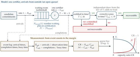
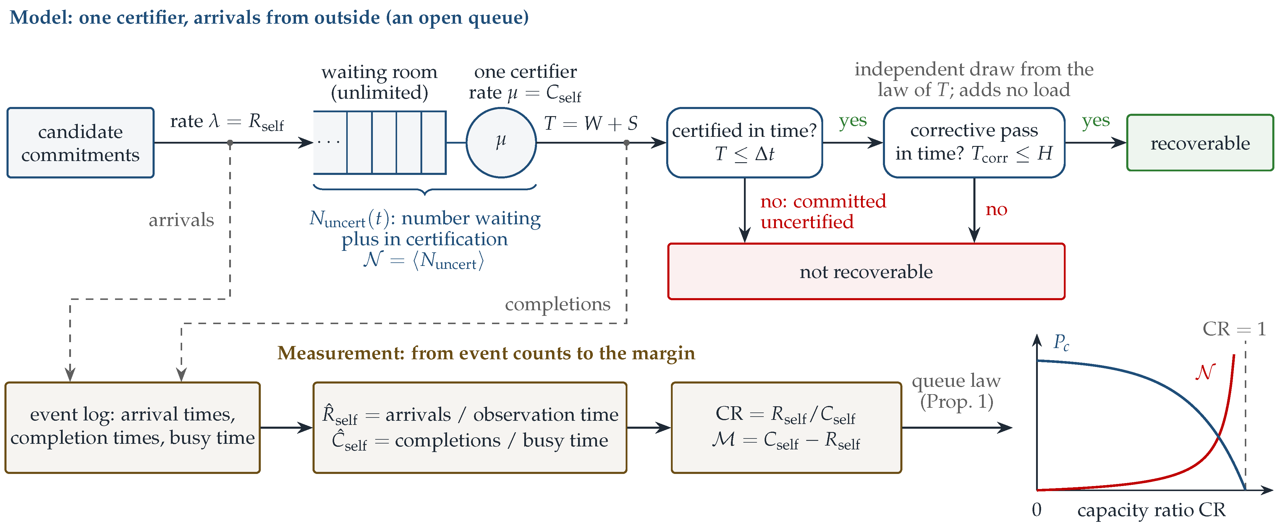
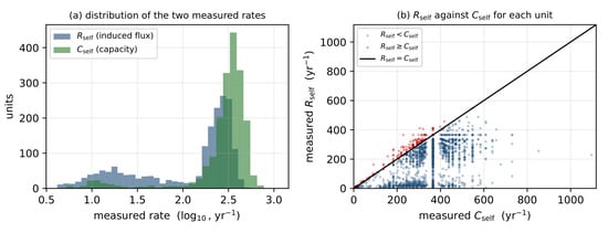
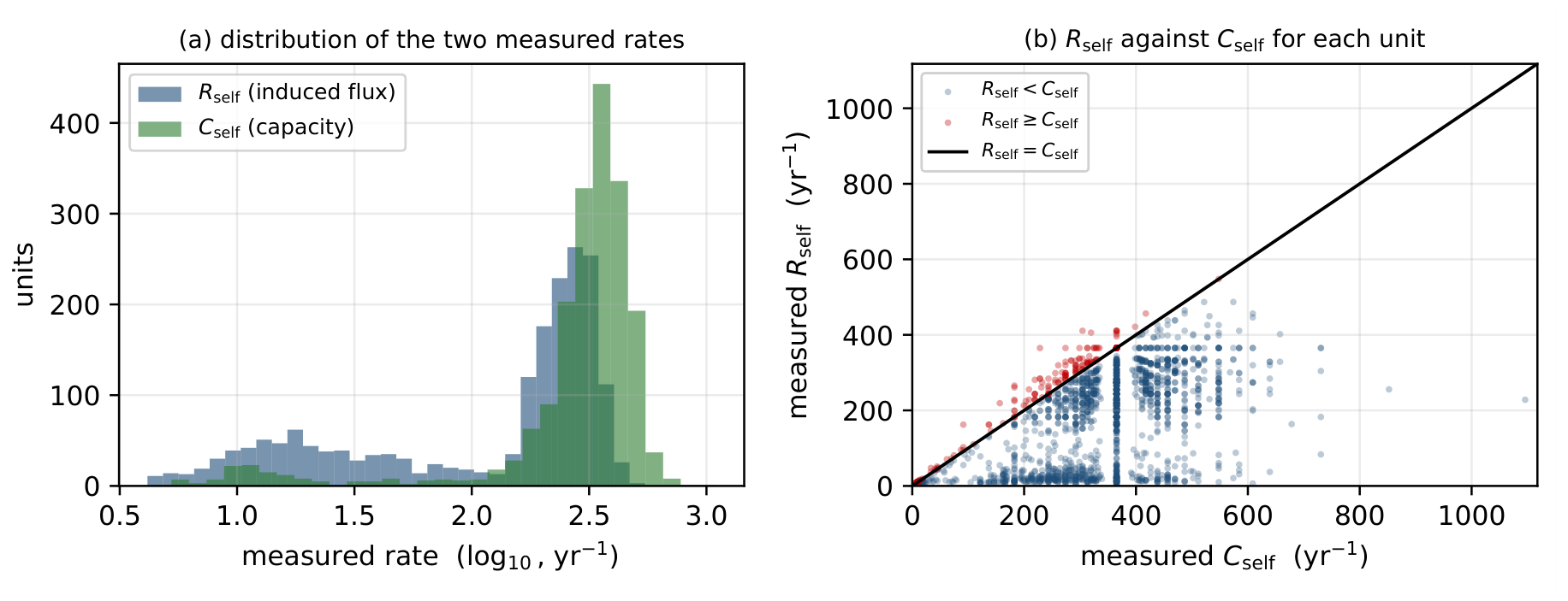
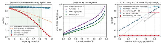
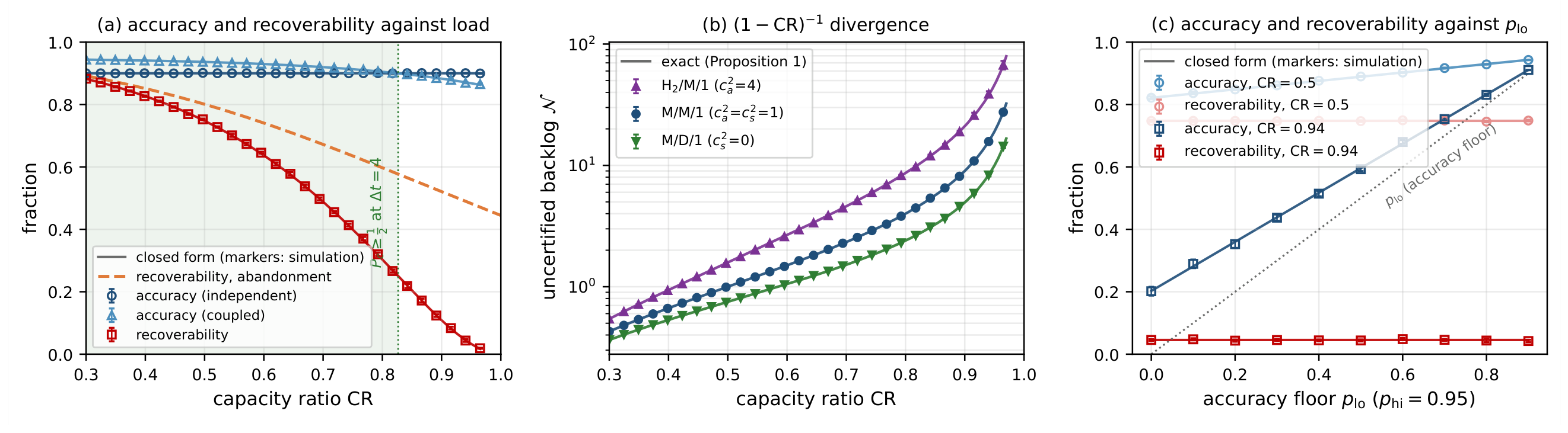

Disclaimer/Publisher’s Note: The statements, opinions and data contained in all publications are solely those of the individual author(s) and contributor(s) and not of MDPI and/or the editor(s). MDPI and/or the editor(s) disclaim responsibility for any injury to people or property resulting from any ideas, methods, instructions or products referred to in the content. |
© 2026 by the author. Licensee MDPI, Basel, Switzerland. This article is an open access article distributed under the terms and conditions of the Creative Commons Attribution (CC BY) license.