Data-Driven Prediction of Photovoltaic System Efficiency: A Case Study of a Rooftop System in Jordan

Abstract

The nature of solar radiation and the high penetration of photovoltaic (PV) systems in the smart electrical grid necessitate the development of models driven by historical operational data capable of precisely estimating the performance of PV systems. In this work, six proposed models are applied to predict the conversion efficiency of a 7.98 kWp rooftop on-grid PV system in Jordan. The dataset comprises 179 daily samples obtained during a single spring–summer period (17 March–24 September 2014). The efficiency modeled is the combined efficiency of the modules and inverter as a system. The proposed models are Decision Tree (DT), Random Forest (RF), Support Vector Machine (SVM), Gradient Boosting (GB), Gaussian Process Regression (GPR), and Elastic Net (EN). The effectiveness of these proposed models is assessed by calculating four performance metrics, namely, the Mean Square Error, prediction accuracy, Coefficient of Determination (R²), and adjusted R², and benchmarking the results with those of six prediction models discussed in our previous work. The results from the unweighted Decision-Making Matrix show that RF showed the best overall performance among the proposed and benchmark models considered. By contrast, the SVM, DT, and GB models exhibited moderate predictive behavior. However, Elastic Net is the worst-performing model among the 12 proposed and benchmark models discussed in this work. Moreover, the RF model’s consistently low prediction error supports its practical utility for PV system performance estimation, despite a slightly higher training cost than simpler models.

1. Introduction

1.1. Machine Learning Algorithms in Solar Photovoltaic Performance Prediction

The widespread adoption of photovoltaic (PV) systems in the smart grid has made PV performance prediction a necessity for grid operators, system designers, and researchers [1], influencing energy management, grid reliability, power quality, scheduling, and economic efficiency [2,3,4]. AI and ML methods are widely used for this task, as they capture complex non-linear relationships between weather parameters and PV output without explicit physical modeling [5]. AI and ML methods often outperform conventional statistical and physical models under variable meteorological conditions [6] and improve via learning [7]. No single method is best for all studies. A method that works well in one context may be worse in another [8,9], and sometimes no method is clearly superior [10,11]. The most common ones are Artificial Neural Network (ANN), Extreme Learning Machine (ELM), traditional/adaptive K-Nearest Neighbor (KNN and A-KNN), Random Forest (RF), Decision Tree (DT), Support Vector Machine (SVM), Gaussian Process Regression (GPR), Gradient Boosting (GB), Elastic Net (EN) and multiple linear regression (MLR).

1.2. Case Studies from Literature

This section outlines significant studies that have employed ML algorithms to predict PV performance. Tree-based methods have been used widely. In [12], a DT regression model was used to find the best input set, a seven-parameter multi-station average, for a large-scale PV system in Pahang, Malaysia, and in [13], a Boosted Decision Tree Regression outperformed the conventional regressors for solar-radiation forecasting in Malaysia.

For Random Forest, combining Smart Persistence with irradiance and prior generation as inputs improved short-term accuracy in Faro, Portugal (nRMSE ≈ 0.25–0.33) [14], while a bagged RF provided one-day-ahead PV output prediction in Australia with built-in cross-validation and robustness to irrelevant inputs [15].

Support Vector Machines have been used to predict the output of a 10 MW station based on module and generation parameters, with low reported error [16]. An SVM regressor tracked the maximum power point more than 94% of the time [17].

XGBoost from the Gradient Boosting family provided the best façade-integrated BIPV power forecasts in Madrid (RMSE of 0.89 and 0.21 kW for south and east arrays) [18], and an Extreme Gradient Boosting Regression with IoT-based logging identified temperature, relative humidity, clear-sky index, and time of day as the most influential inputs [19].

In the case of Gaussian Process Regression, a Bayesian-optimized GPR was found to outperform neural network baselines for short-term forecasting in Canberra, Australia [20], while GPR with a squared-exponential kernel achieved the best accuracy among the kernels tested on an Algerian on-grid system [21].

Regarding Elastic Net, a comparison of 19 linear regression models found that EN was not able to accurately predict power, current, or voltage for two PV modules in Iran [22]. However, EN combined with Bayesian Density Estimation achieved a lower MAE and RMSE than ANN, SVM, RF, and Gradient Boosting machines on large Indian datasets [23].

1.3. Significance of This Work

In this context, the original contributions of this research work are summarized as follows:

• The development of various ML techniques, ranging from simple linear models to complex non-linear data-driven approaches, for estimating a PV system’s performance based on historical weather data and operational conditions.
• The evaluation of the models’ effectiveness and a fair comparison among them aim to identify the best-performing model in terms of efficiency and reliability, which would make it an attractive choice for real-world applications.
• The validation of the investigated models on a real case study involving a 7.98 kWp on-grid PV system installed at the Hashemite University, Jordan. The dataset contains 179 daily samples collected between 17 March and 24 September 2014. The estimation is carried out for the modules and inverter as a combined system.

This study evaluates six additional machine learning models (DT, RF, SVM, GB, GPR and EN) on the same dataset and partition as analyzed in our previous efforts on this system, including the assessment of multiple linear regression and neural network models [24,25] and, more recently, an adaptive K-Nearest-Neighbor model [26]. All twelve models are compared within a single unified framework using an unweighted decision matrix and a performance-gain analysis against a common baseline. Comparative studies change the dataset or the protocol across models. The controlled same-data comparison used here isolates the effect of the learning algorithm itself.

This work is organized as follows: Section 2 presents the experimental setup, and Section 3 describes the data collection and analysis process. Section 4 presents brief ideas about the six proposed prediction models in this paper. Results and discussions are presented and explored in detail in Section 5. Finally, conclusions and future works are highlighted in Section 6.

2. Experimental Setup

To achieve this project’s objective, a 7.98 kWp grid-tied photovoltaic system was installed on the rooftop of the president’s building at Hashemite University (HU) in Zarqa, Jordan. Table 1 summarizes the technical requirements of this photovoltaic system, and Table 2 includes the actual dates of rainy days and cleaning days of the system. The global horizontal irradiance (GHI) was measured using a pyranometer mounted on the rooftop next to the PV array. The ambient temperature was measured using a shielded thermistor. The AC output energy of the inverter was also recorded. The total daily incident energy per unit area used in Equation (1) was obtained by integrating instantaneous irradiance samples over each day. Consequently, the changing solar angle of incidence throughout the day is already included in the daily total. The PV modules are 285 W_p polycrystalline modules, and the inverter is a 3-phase 8 kW string inverter (see Table 1 for specifications). Hence, the modeled efficiency η is a system-level quantity that takes into account module and inverter losses. The effectiveness of the system is determined in the following way:

$$\eta = {\displaystyle \frac{E_{out}}{I \times A}}$$

(1)

where $\eta$ represents the conversion efficiency of the PV system; $E_{out}$ indicates the net AC output energy; $I$ represents the total daily global incident irradiance; and $A$ indicates the total area of the PV modules (=49.061 m²).

Table 1. Technical specification of the PV system employed in this study.

Parameter	Value
Latitude	32.10° N
Longitude	36.18° E
Altitude	575 m
Number of PV modules	28
Nominal power of each module	285 Wp
Number of strings	2
Tilt angle	26°
Azimuth angle	0°
Number of inverters	1
Nominal power of inverter	8 kW (3-phase)

Table 2. Cleaning days during the experiment.

Cleaning Number	Cleaning Dates	Cleaning Type
1	17 March 2014	Naturally by heavy rainfall
2	8 May 2014	Naturally by heavy rainfall
3	12 July 2014	Manually
4	24 September 2014	Manually

The quantity to be modeled is the daily conversion efficiency $\eta$ rather than the AC output energy $E_{out}$ directly. The conversion efficiency is a dimensionless indicator of the system that isolates the effect of dust accumulation and temperature on the array–inverter chain and is comparable between days with very different irradiance. In operation, the $\eta$ forecast can be combined with a separate daily forecast of the incident irradiance, $I$, using Equation (1) to obtain the expected AC output, $E_{out}=\eta \times I\times A$. Operationally, this decoupling is convenient and consistent with how performance is reported in our previous work on this system [24,25,26]. We recognize that $\eta$ and $I$ are not completely independent; there is a weak intrinsic dependence of module efficiency on irradiance and a stronger dependence on cell temperature, which is correlated with irradiance. However, the main limitation of the approximation of treating $\eta$ and I as separable is the issue discussed in Section 6.1.

3. Data Collection/Analysis

The collected dataset includes $N=192$ data points (which are the number of days during the period of the experiment) of pairs of inputs and outputs of daily conditions of the PV system. The inputs comprise the following:

• The counter of the dust accumulation/exposure days (labeled as $D$ in chronological order).
• The average daily ambient temperature (expressed as $T$ in °C).

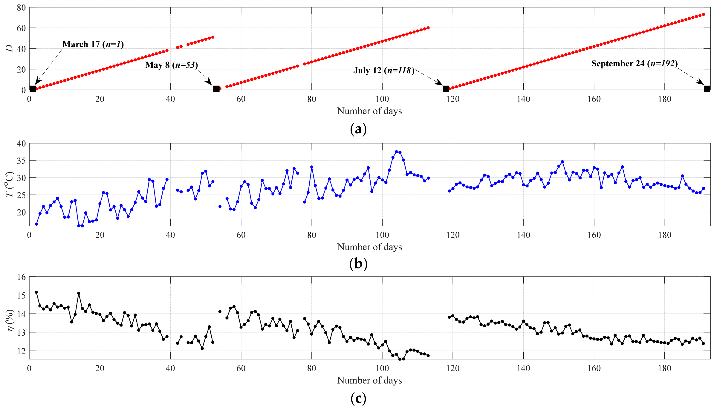
However, the output is the daily measured conversion of the PV system’s efficiency (hereafter denoted as $\eta$ in %). The following data points are removed from the $N=192$ data points: nine outliers (spiked values of efficiency were found due to sensor faults) and four cleaning days. Nine of the 13 excluded points are due to physically implausible efficiency spikes caused by sensor faults, and the remaining four are due to cleaning days. These are measurement artifacts and discrete maintenance events, not normal operating conditions, so their removal (~6.8% of the 192 raw records) should not bias the learned relationship over the remaining 179 points. The nine outliers are spread over the period from D = 39 to D = 120; the four cleaning days are 17 March, 8 May, 12 July, and 24 September 2014.

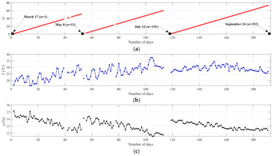
After the 13 data points above are removed, 179 remain for further analysis. Figure 1a–c show the D, the T, and the η, respectively, for the entire experiment period (N = $192$ data points, excluding outliers and cleaning days). In Figure 1c, negative correlations are shown between $D$ and $\eta$ (because the dust accumulation on the PV modules blocks sunlight from reaching the solar cells) and between $T$ and $\eta$ (due to the negative temperature coefficient) [27,28,29]. Moreover, as expected, there are sudden jumps in the $\eta$ during the PV system’s cleaning days. Both predictors have physical significance. The within-cycle efficiency decay is due to the cumulative effect of dust accumulation (D), which induces progressive optical attenuation at the module surface, and increasing ambient temperature ($T$), which reduces efficiency due to the modules’ negative temperature coefficient. The two are in the same direction between cleanings. Using the typical crystalline-silicon temperature coefficient of −0.4%/°C, the ~10 °C temperature increase observed in the first cycle alone accounts for on the order of half of the observed decay. So, the two mechanisms are of similar magnitude in this dataset. As the model uses only these two physically motivated inputs, no automatic feature selection is performed, and the relevance of each input is already apparent from the correlation structure in Figure 1.

Figure 1. The input–output pairs for $N=192$ data points: (a) $D$, (b) $T$, and (c) $\eta$.

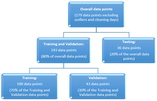
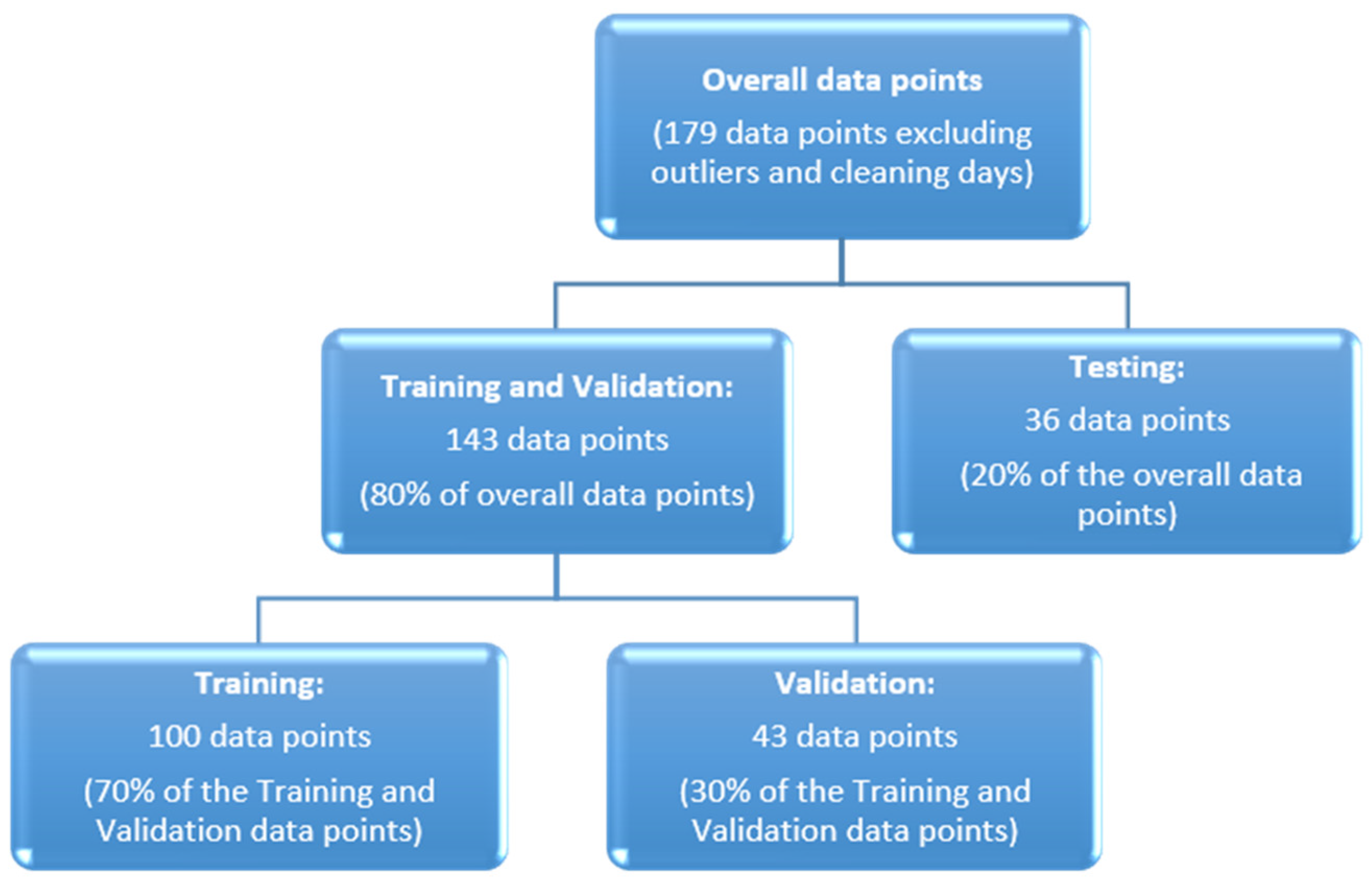
The dataset (N = 179) is split into 80% (143 points) for training and validation and 20% (36 points) for testing. The 143 points are then divided into 70% for training ($N_{train}$ = 100) and 30% for validation ($N_{valid}$ = 43), where the training subset is randomly sampled and used to tune the model configurations. The benchmark and proposed models are evaluated on the 36 held-out test points on metrics defined later in this paper. Figure 2 illustrates the categorization of the data points in this study.

Figure 2. The classification of the data points followed in this work.

4. Methodology

This section provides a brief summary of the prediction models used in this study and the metrics used to assess their performance. The discussion centers on the newly proposed models, whereas the benchmark models—specifically, Multivariate Linear Regression (MLR), Artificial Neural Network (ANN), Extreme Learning Machine (ELM), and traditional/adaptive K-Nearest Neighbor (KNN and A-KNN)—were comprehensively analyzed and delineated in our previous research [24,25,26]. Thus, instead of reiterating their theoretical foundations, Section 4 presents and examines only their respective results for comparative analysis [26].

4.1. Brief Description of the Proposed Prediction Models

4.1.1. Decision Tree (DT)

DT is a parameter-free supervised learning algorithm which can be used for both regression and classification problems. It works by dividing the feature space into smaller and smaller groups of similar characteristics, which leads to a hierarchical tree-like structure that is easy to understand and works well with computers [30,31]. To enhance the predictive power and reduce the overfitting of the DT model, Bayesian optimization (BO) [32] was used for optimization. Tuning was performed on three important hyperparameters: minimum leaf size, maximum number of splits, and number of variables sampled at each node.

4.1.2. Random Forest (RF)

RF is an ensemble learning method that combines the predictions of multiple decision trees. Each tree is constructed independently via bootstrap sampling and random feature selection. For regression tasks, the final output is the average prediction of all the trees [33]. This architecture is robust against overfitting and enables the processing of high-dimensional data. The RF model was built using the bagging method and tuned on three key hyperparameters: the number of learning cycles, the minimum leaf size, and the number of variables sampled per iteration. Once again, we implemented BO to systematically explore the hyperparameter space and find the optimal balance between model complexity and generalization performance [34].

4.1.3. Support Vector Machine (SVM)

Support Vector Machine, in its regression form (SVR), is a supervised learning algorithm that fits the function to the target values within a certain threshold by using a kernel. It also guarantees that the learned function is as flat as possible [35,36]. This paper uses kernel functions to project the inputs into higher-dimensional feature spaces, thus making it suitable for linear and non-linear regression problems. In this research, the prediction accuracy has been improved, and the generalization ability has been maintained by optimizing the box constraint, epsilon value and kernel function selection of the SVR model using BO.

4.1.4. Gradient Boosting (GB)

GB is a sequential ensemble learning method that iteratively combines several weak learners, usually shallow decision trees, into a strong predictive model. Each new learner is trained to correct the previous learner’s errors [37,38]. This formulation makes GB particularly good at identifying complex interactions among variables and non-linear relationships in the data. The GB model was implemented in this study using the LSBoost method, which minimizes least-squares loss, and was optimized for the smallest leaf size, learning rate, and total number of trees in the ensemble. Here, BO was also used to tune these hyperparameters, automatically finding a good trade-off between model predictive performance and performance on new data.

4.1.5. Gaussian Process Regression (GPR)

GPR is a Bayesian inference-based nonparametric and probabilistic regression method. Rather than fitting a single deterministic model, it models a distribution over possible functions [39]. This enables GPR to generate not only point predictions but also well-calibrated uncertainty estimates. This is particularly useful for small- to medium-sized datasets where it is important to measure prediction confidence and capture non-linear trends [40]. Here, we apply BO to optimize the GPR model. The main tuning parameters were the kernel function, basis function, and noise level. This enabled more accurate predictions while still allowing the model to quantify uncertainty.

4.1.6. Elastic Net (EN)

EN is a linear regression method that simultaneously uses L1 (Lasso) and L2 (Ridge) penalty terms. Thus, you can select variables and shrink coefficients at the same time [41]. This dual-penalty formulation is particularly helpful when there is multicollinearity among predictors or when there are more features than observations. We systematically varied the mixing parameter α to allow a flexible trade-off between the L1 and L2 regularization components. We determined the optimal regularization strength, λ, using 10-fold cross-validation. We considered a single strong evaluation sufficient because the EN fitting procedure is deterministic and internally cross-validated, and we did not perform repeated trials with different random data splits.

4.2. Performance Metrics

Similar to [29], this study considers four performance metrics to evaluate the effectiveness of the proposed models against the benchmark models on the test dataset (${\mathbf{X}}_{test}$) in addition to the computational effort required while developing the prediction models. These metrics are the following.

4.2.1. Accuracy (Accuracy)

The accuracy metric designates the average closeness between the estimated and actual daily conversion efficiency, $\eta$, and is defined using the absolute prediction error in Equation (2); defined this way, it is equivalent to one minus the mean absolute percentage error (1 − MAPE), and the absolute deviation ensures that positive and negative errors do not cancel each other out. The higher the accuracy value, the more effective the prediction model:

$$Accuracy={\displaystyle \frac{1}{N_{test}}}{\displaystyle \sum _{i=1}^{N_{test}}}(1-{\displaystyle \frac{\left|{\eta }_i-{\widehat{\eta }}_i\right|}{{\eta }_i}}) \times 100\%$$

(2)

where ${\widehat{\eta }}_i$ and ${\eta }_i$ are the $i$-th estimated and actual daily system’s conversion efficiency, respectively, and $i=1,\dots ,N_{test}$. The higher the values of accuracy, the more effective the prediction model.

4.2.2. Mean Square Error (MSE)

The MSE estimates the average squared difference between the estimated ($\widehat{\eta }$) and actual ($\eta$) daily system’s conversion efficiency provided by all the proposed and benchmark prediction models, and it is expressed as follows:

$$MSE= {\displaystyle \frac{1}{N_{test}}}{\displaystyle \sum _{i=1}^{N_{test}}}{\left({\eta }_i-{\widehat{\eta }}_i\right)}^2$$

(3)

where ${\widehat{\eta }}_i$ and ${\eta }_i$ are the $i$-th estimated and actual daily system’s conversion efficiency, respectively, and $i=1,\dots ,N_{test}$. Based on Equation (3), the smaller the values of MSE, the more effective the prediction model.

4.2.3. Coefficient of Determination ($R^2$) and the Adjusted Version ($R_{adjusted}^2$)

The $R^2$ and its adjusted version ($R_{adjusted}^2$) express the variability of the dependent variable (i.e., output; daily system’s conversion efficiency in this work) estimated by the prediction models and produced by the independent variables (i.e., the inputs that represent dust accumulation and the average ambient temperature in this work). They are presented by Equations (4) and (5), respectively:

$$R^2=\left[1-{\displaystyle \frac{{\sum }_{i=1}^{N_{test}}{\left({\eta }_i-{\widehat{\eta }}_i\right)}^2}{{\sum }_{i=1}^{N_{test}}{\left({\eta }_i-\overline{\eta }\right)}^2}}\right] \times 100\%$$

(4)

$$R_{adjusted}^2=\left[1-\left({\displaystyle \frac{{\sum }_{i=1}^{N_{test}}{\left({\eta }_i-{\widehat{\eta }}_i\right)}^2}{{\sum }_{i=1}^{N_{test}}{\left({\eta }_i-\overline{\eta }\right)}^2}}\right)\left({\displaystyle \frac{N_{test}-1}{N_{test}-3}}\right)\right]\times 100\%$$

(5)

where ${\eta }_i$ and ${\widehat{\eta }}_i$ are the $i$-th actual and estimated daily system’s conversion efficiency, respectively, $i=1,\dots ,N_{test}$, and $\overline{\eta }$ is the average value of $\eta$. An R² value of 100% means that the chosen independent variables, which are dust accumulation and average ambient temperature, can fully explain the variability of the dependent variable. This means that there are no other factors that could have affected the output. On the other hand, a R² value below 100% means that other factors outside of the ones used in the model also affect the dependent variable’s variability, but they have not been included in the current modeling framework [24]. Because the number of predictors is p = 2 (dust accumulation days, D, and average ambient temperature, $T$), the adjusted R² in Equation (5) uses the correction factor ($N_{test}-1)$/($N_{test}-p-1$). Because every model uses the same two predictors, adjusted R² is a strictly monotonic transformation of R² and ranks the models identically; it is reported for completeness rather than as an independent criterion.

Each cross-validation (CV) simulation trial has its own set of performance metrics that are calculated. After gathering all the metrics for each trial, the mean values are calculated and used to compare models.

Finally, we use a performance gain (PG) metric for each of the evaluation criteria listed above—MSE, accuracy, R², and adjusted R²—to measure how much better each prediction model is than the least accurate one. The PG is calculated only for the proposed models, with the model that does the worst being the baseline (BL). It is shown as follows:

$$P{G}_{MSE}=\left|{\displaystyle \frac{{MSE}^{Proposed}-{MSE}^{BL}}{{MSE}^{BL}}}\right|\times 100\%$$

(6)

$$P{G}_{Accuracy}=\left|{\displaystyle \frac{{Accuracy}^{Proposed}-{Accuracy}^{BL}}{{Accuracy}^{BL}}}\right|\times 100\%$$

(7)

$$P{G}_{R^2}=\left|{\displaystyle \frac{{R^2}^{Proposed}-{R^2}^{BL}}{{R^2}^{BL}}}\right|\times 100\%$$

(8)

$$P{G}_{R_{adjusted}^2}=\left|{\displaystyle \frac{{R_{adjusted}^2}^{Proposed}-{R_{adjusted}^2}^{BL}}{{R_{adjusted}^2}^{BL}}}\right|\times 100\%$$

(9)

5. Results and Discussion

This section presents the development, application, and comparison results of the benchmark and proposed prediction models.

5.1. Benchmark Prediction Models

The benchmark prediction models are discussed in detail in [24,25,26]. The most critical features and results are briefly summarized in this section.

5.1.1. Multivariate Linear Regression (MLR)

In [24], MLR analysis is used to establish the mathematical relationship between D and T (i.e., independent variables) and η (i.e., dependent variable), based on the collected data (which consisted of $N=$ 143 observations). Then, the best mathematical equation that represents these data is used to estimate the $\eta$ of each $k$-th test pattern of the test dataset (${\mathbf{X}}_{test}$), $k=1,\dots ,N_{test}$, using the corresponding input test patterns, $D_k$ and $T_k$.

It is worth noting that the computational efficiency of the models will be reported and discussed in this work. MLR took 1.41 s to establish the best mathematical equation in terms of the computational effort of the MLR model. The MLR fit reported in [24,25] on this system yields a coefficient on the ambient temperature term corresponding to a system-level thermal sensitivity of about −0.3 to −0.4% of efficiency per °C, consistent with the typical temperature coefficient of maximum-power for crystalline-silicon modules (−0.35 to −0.45%/°C) reported in the module-degradation literature [27,28]. The coefficient of the dust accumulation term is of the same magnitude for each cleaning cycle, as predicted by the decomposition in Section 3, which indicates that the two inputs have similar contributions to the variation observed in $\eta$.

5.1.2. Artificial Neural Networks (ANNs)

The first version of the ANN prediction model (hereinafter referred to as ANN₁) was developed in [24] using 143 data points with the scaled conjugate gradient back-propagation algorithm, with an RMSE of 10^–5 and a maximum of 100 training epochs. Also, two hidden layers with 10 and 4 hidden neurons were used, respectively. The second version of the ANN prediction model (hereafter referred to as ANN₂) was established in [25] as an improvement over ANN₁ [24], developed for the same purpose. The ANN₂ had one hidden layer with 22 neurons and the “poslin” (ReLU) activation function. As with the ANN₂ model in [25], the ELM model was optimized with respect to the number of hidden neurons and the choice of activation function. The best ELM model was found to be the one with 700 neurons and the activation function “Triangular Basis”. The computational effort was much higher (e.g., >40 min for the ELM model) because of the complexity of ANN₁, ANN₂, and ELM compared to MLR. Likewise, the ANN₁, ANN₂, and ELM benchmark models were used to estimate the system’s conversion efficiency on the test dataset and compared with the MLR model.

5.1.3. Traditional and Adaptive KNN Models

Regarding the traditional and adaptive KNN (KNN and A-KNN, respectively) prediction models discussed in detail in [26], the same 1$43$ data points have been selected to establish the training and validation datasets, respectively. The prediction models required 3.56 s to identify the optimal number of nearest neighbors and estimate the conversion efficiency of the test dataset. After the optimal K is determined, it is used to calculate the system’s conversion efficiency on the test dataset.

5.2. Discussion of the Proposed Prediction Models

The investigated models were optimized using BO with 30 iterations, involving the systematic tuning of key hyperparameters, as clarified in Section 4. Specifically:

• DT was optimized in terms of the minimum leaf size, maximum number of splits, and number of variables to sample. The optimization explored a wide range of values: minimum leaf size varied from 1 to 25, the maximum number of splits ranged from 5 to 100, and the number of variables to sample at each split was set between 1 and 4. It took ~0.41 min to identify the optimal model configuration and estimate the conversion efficiency on the test dataset.
• RF was optimized in terms of the minimum leaf size, number of trees in the ensemble, and number of variables to sample. The optimization explored a wide range of values: the minimum leaf size varied from 1 to 25, the number of trees in the ensemble ranged from 30 to 300, and the number of variables to sample at each split was set between 1 and 4. It took ~43.7 min to identify the optimal model configuration and estimate the conversion efficiency on the test dataset.
• The SVM regressor was optimized in terms of the box constraint, epsilon value, kernel function, and kernel-specific settings. The optimization explored a wide range of values: the box constraint varied from 0.01 to 200, epsilon values ranged from 0.001 to 0.4, and three kernel types were explored: linear, Gaussian, and polynomial. For the latter two kernel types, the kernel scales ranged from 0.01 to 20, while polynomial kernels were further tuned with orders 2, 3, and 4. It took ~1.75 min to identify the optimal model configuration and estimate the conversion efficiency on the test dataset.
• GB was optimized in terms of the minimum leaf size, learning rate, and number of trees in the ensemble. The optimization explored a wide range of values: minimum leaf size varied from 1 to 15, learning rate ranged from 0.005 to 0.3, and the number of trees was set between 30 and 200. It took ~54 min to identify the optimal model configuration and estimate the conversion efficiency on the test dataset.
• GPR was optimized in terms of the kernel function, basis function, and noise level (sigma). The optimization explored five different kernel functions, namely, squaredexponential, matern32, matern52, exponential, and rationalquadratic, along with four types of basis functions, namely, constant, linear, pureQuadratic, and none. Furthermore, the noise level (sigma) was varied over a wide range, from 0.01 to 10. It took ~2.87 min to identify the optimal model configuration and estimate the conversion efficiency on the test dataset.
• EN was optimized in terms of the mixing parameter (α). The optimization explored a wide range of α values, from 0.01 to 0.99. It took ~0.82 min to identify the optimal model configuration and estimate the conversion efficiency on the test dataset.

All models were developed and implemented using MATLAB^® R2024a and executed on a personal computer equipped with an 11th Gen Intel^® Core™ i5-1135G7 processor (2.40 GHz), 8.00 GB of RAM, and a 64-bit Windows operating system. To support reproducibility, the inputs were normalized prior to training, and the same random seed was fixed for all data partitioning and stochastic model components.

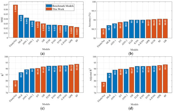
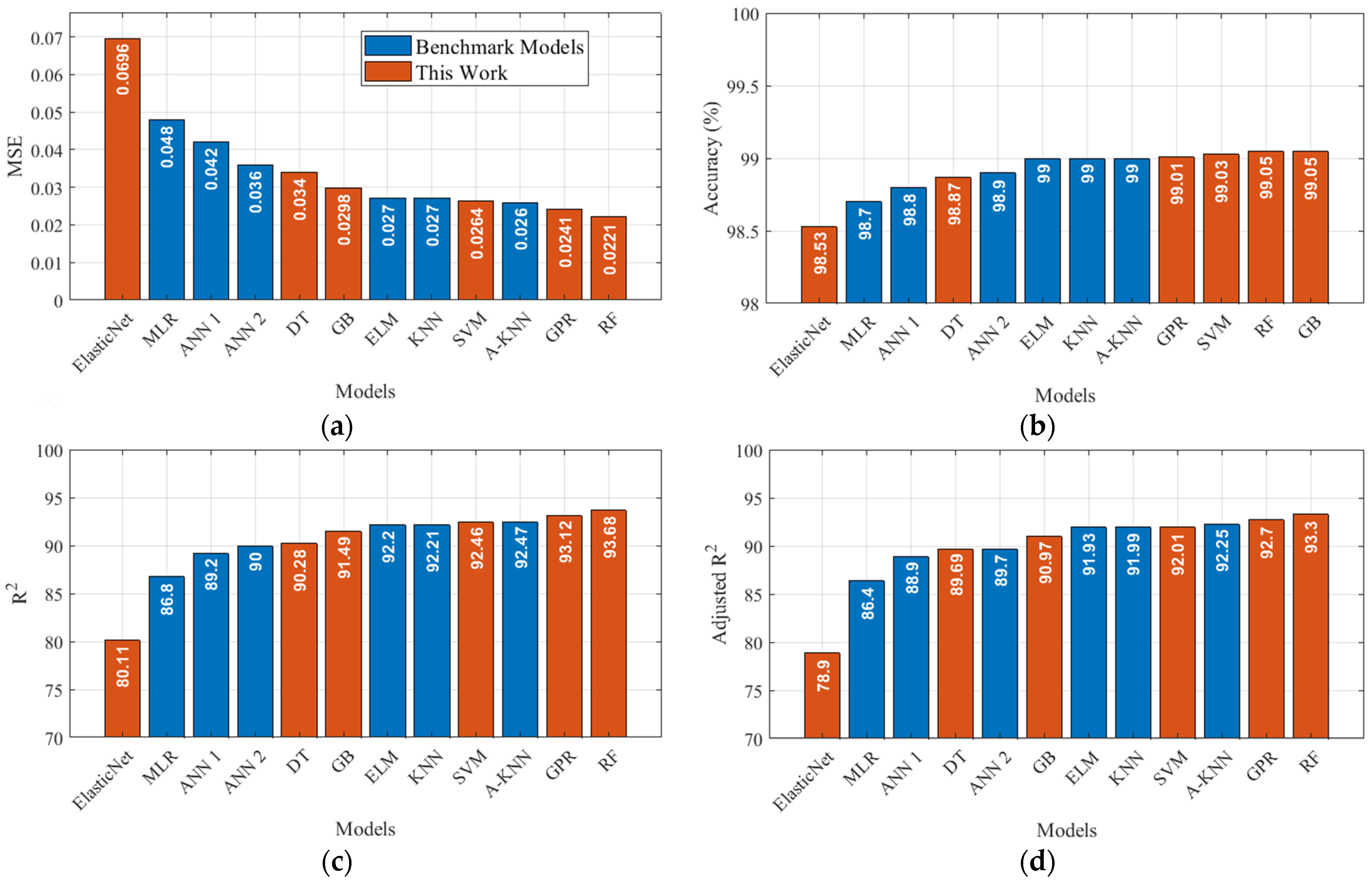
Using the same 143 data points selected for the training and validation and the same 36 data points chosen for the testing of the benchmark prediction models, the six proposed models in this work (RF, DT, SVM, GPR, GB, and EN) have been trained, validated, and tested accordingly to ensure consistency in the evaluation. Figure 3 presents the results of the proposed models in this study compared with the benchmarks. The results are on the 36 test datasets. Figure 3 presents a comprehensive performance comparison between benchmark models (blue bars) and newly proposed models (orange bars) across four critical evaluation metrics—accuracy, MSE, R², and adjusted R²—utilizing Equations (2)–(5). Each of these metrics provides a unique perspective on model performance, which is essential for a comprehensive understanding of predictive effectiveness and robustness across the test dataset.

Figure 3. Comparison results of the proposed prediction model to the benchmark prediction models: (a) MSE, (b) accuracy, (c) R², and (d) $R_{adjusted}^2$.

By inspecting Figure 3, a few observations can be highlighted and discussed. In Figure 3a, an illustration of the MSE is presented, which quantifies the average squared difference between the actual and predicted conversion efficiency. Lower values indicate better prediction and vice versa. It is noted that RF and GPR, the proposed models in this work, exhibit the lowest MSE values of 0.0221 and 0.0241, respectively. These results suggest that the models achieved the lowest errors among the models considered, which makes them well suited to this regression task. However, EN, another proposed model, achieves the highest MSE of 0.0696, significantly worse than all benchmark models, including MLR, which has an MSE of 0.048. This suggests poor predictive alignment with actual conversion efficiency values due to model misspecification. In addition, models such as ANN₁, ANN₂, DT, GB, ELM, KNN, SVM, and A-KNN have MSEs clustered between 0.026 and 0.042, which indicates reasonable to intermediate prediction accuracy. These models demonstrate a transition from linear to non-linear regression, offering trade-offs between simplicity and accuracy.

Accuracy is shown in Figure 3b, referring to the proportion of predictions falling within a defined error tolerance. Higher values denote better prediction. GB and RF (proposed models in this work) achieve the highest recorded accuracy of 99.05%, while SVM and GPR (also newly proposed models) closely follow with 99.03% and 99.01%, respectively, reflecting high predictive reliability. The proposed model EN again underperforms with the lowest accuracy of 98.53%. While the numerical difference may appear minor, in high-precision applications, such performance gaps can be critical. DT and all the benchmark prediction models in this study (MLR, ANN₁, ANN₂, ELM, KNN, and A-KNN) achieve accuracies of 98.7–99.0%, which reflects moderate performance. These models strike a balance but lag behind the more robust ensemble-based approaches.

Figure 3c displays R², which represents the proportion of variance in the target variable explained by the model. A value closer to 100% means a stronger model fit. RF (proposed) stands out with the highest R² value of 93.68%, followed by GPR (93.12%) and A-KNN (92.47%). These models explain a large proportion of the variance in this dataset, which indicates a good fit. However, EN shows an R² of 80.11%, which is the lowest in this experiment. This is followed by MLR, a benchmark model with an R² of 86.8%, which suggests a limited ability to capture complex patterns. Moreover, the SVM, KNN, A-KNN, and DT models achieve R² values ranging from 90% to 92.5%, which indicates strong explanatory power. These are preferable in scenarios, where ensemble methods, such as RF/GB, might be computationally intensive.

Lastly, Figure 3d shows the adjusted R², which adjusts R² for the number of predictors in the model, offering a more conservative estimate, especially for complex models. The reduction in adjusted R² relative to R² suggests potential overfitting or the irrelevance of some predictors. RF again leads with an adjusted R² of 93.3%, followed by GPR (92.7%) and A-KNN (92.25%). These results are consistent with a good fit of the top models on this dataset. The proposed EN model shows the lowest adjusted R² (78.9%), which indicates not only poor fit but also inefficiency in handling model complexity. Models such as MLR, ANN₁, DT, and ANN₂ yield adjusted R² values in the 86.4–89.7% range, offering a good balance between model complexity and explanatory power. However, models such as GB, ELM, KNN, and SVM have adjusted R² values closer to those of the top models, which indicates commendable performance.

The unweighted Decision-Making Matrix (DMM) is presented in Table 3. It is highly important to objectively assess and benchmark the prediction model performance on the basis of multiple statistical metrics, as no single metric can give a comprehensive picture of a model’s efficiency. Therefore, a multi-criteria decision matrix offers a systematic approach to integrating multiple evaluation indicators into a single performance index. This provides a sound basis for comparison between the proposed and benchmark prediction models to guide the selection of the most appropriate prediction model(s). The evaluation was based on four basic criteria: MSE, accuracy, R², and $R_{adjusted}^2$.

Table 3. Decision Matrix (Ranking Matrix).

Criteria	MSE		Accuracy		R2		${\mathit{R}}_{\mathbf{adjusted}}^{\mathbf{2}}$		Rank
Model	Value	Score	Value	Score	Value	Score	Value	Score
RF	0.0221	1	99.05	1	93.68	1	93.3	1	1
GPR	0.0241	2	99.01	2	93.12	2	92.7	2	2
SVM	0.0264	2	99.03	2	92.46	2	92.01	2	2
A-KNN	0.026	2	99	2	92.47	2	92.25	2	2
KNN	0.027	3	99	2	92.21	3	91.99	3	2.75
ELM	0.027	3	99	2	92.2	3	91.93	3	2.75
GB	0.0298	4	99.05	1	91.49	4	90.97	4	3.25
DT	0.034	4	98.87	4	90.28	4	89.69	5	4.25
ANN2	0.036	5	98.9	4	90	5	89.7	4	4.5
ANN1	0.042	5	98.8	5	89.2	5	88.9	5	5
MLR	0.048	5	98.7	5	86.8	5	86.4	5	5
EN	0.0696	6	98.53	6	80.11	6	78.9	6	6

In this approach, each model is scored for each criterion, and the ranks range from 1 to 6, where 1 is the best performance and 6 is the worst. The best and worst models are considered outliers, with the best model scoring 1 and the worst model scoring 6. The performance of the other 10 models is plotted as a distribution and compared across four quartiles. Models in the first quartile receive a score of 2, the second quartile a score of 3, the third quartile a score of 4, and the fourth quartile a score of 5. This is done for all four criteria. Because MSE, R², and adjusted R² are algebraic transformations of each other over a fixed test set, MSE and R² were found to rank the models in the same way. Thus, the matrix is constructed based on two independent criteria, the squared-error criterion (MSE) and accuracy criterion (1 − MAPE), with R² and adjusted R² reported for reference only. The models are ranked for each criterion, and the best and worst models are treated as boundary cases, scoring 1 and 6, respectively. The other ten models are spread across the interquartile range and are scored by quartiles (first quartile: 2, second: 3, third: 4, fourth: 5). The average points score of each model is the arithmetic mean of its scores per criterion. The final ranking is based on the ascending order of the average points, i.e., the lower the value, the better the overall performance of the model.

Then we calculated an average points score, which is the arithmetic mean of the four rankings per model. The final ranking was obtained by sorting the models in increasing order of their average points, where a lower average indicates better overall performance.

As shown in Table 3, RF achieved the best performance in all evaluation dimensions and was ranked first in all criteria. GPR, SVM, and A-KNN were ranked second, with very close scores across all criteria. KNN and ELM have very similar performance and are followed by GB. Performance shows a clear degradation for DT and ANN₂, whereas ANN₁ and MLR perform worse. The worst performance of EN across all criteria, for this dataset, is a clear outlier, with a score significantly lower than that of any of the other eleven models. It is important to note that MSE and R² have the same ranking behavior, which may suggest that it is sufficient to calculate only one of them for the performance analysis. Given the limited test set ($N_{test}=36$), small differences between closely ranked models should be read with caution: RF, GPR, and SVM form a comparable group whose separations lie within the observed run-to-run variability, whereas Elastic Net underperforms every other model on every criterion by a margin well beyond it.

The improved results of RF on this dataset can be explained by the construction of RF: it averages over many decorrelated bootstrap trees to reduce variance and capture the mild non-linearity of the two-feature response while maintaining stability on a small sample. This is something that the linear Elastic Net cannot do and that a single decision tree does less reliably, which agrees with the ordering here.

It is helpful to separate the cost of one-time offline training from the cost of online inference. The reported tuning times (e.g., ~43.7 min for RF, ~54 min for GB) are only incurred during Bayesian optimization; once trained, prediction is effectively instantaneous for all six models on the same hardware, so each is applicable in real time. In terms of scalability, the ensemble methods (RF, GB) have the highest training cost, and the single tree and linear models the lowest. The low-cost models (DT, EN) are suitable for frequent retraining or minimal-budget settings, while the higher-accuracy models (RF, GPR) are appropriate for periodic server-side retraining where accuracy is the priority. Future work will include scalability to larger multi-site datasets and a dedicated hardware/latency study.

5.3. Performance Gain

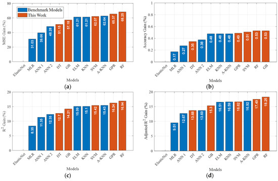
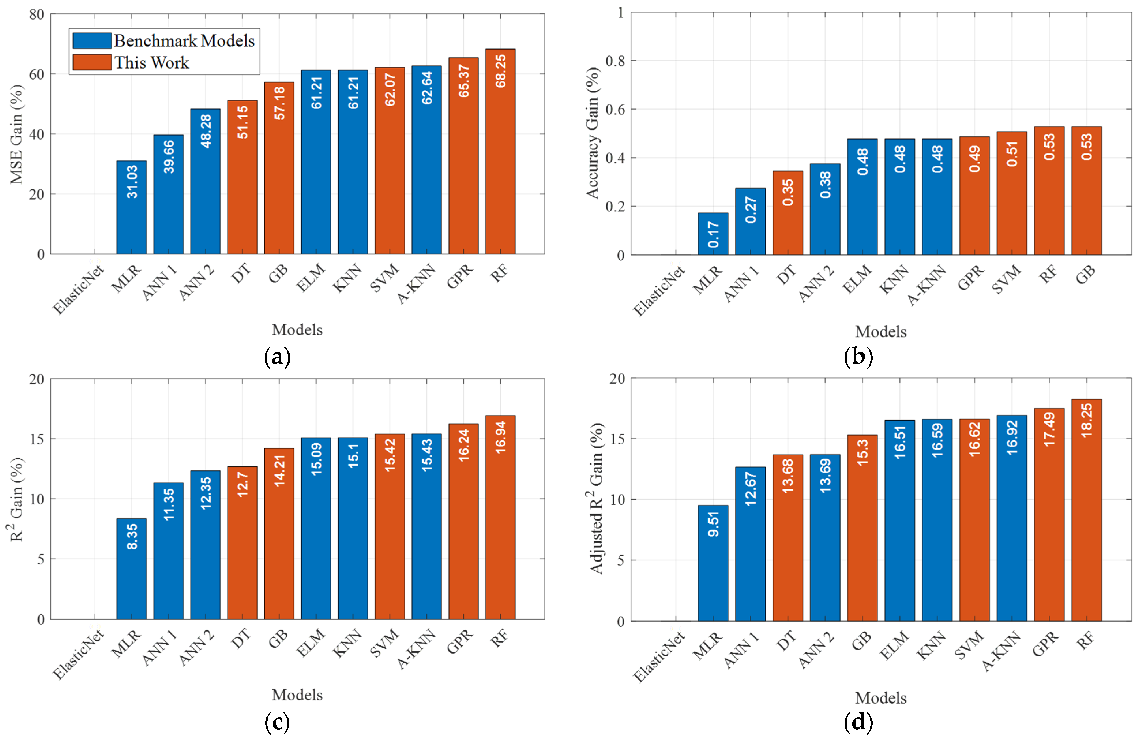
To demonstrate the effectiveness of the proposed prediction model compared to the other benchmarks, the performance gain ($PG$) of each performance metric is calculated using Equations (6)–(9), and the results are displayed in Figure 4. The EN is considered a baseline. Following the estimation of the performance of the proposed prediction models alongside other benchmark models using the four selected metrics, the following comments can be made:

Figure 4. The performance gain of each performance metric for the benchmarks and proposed prediction models: (a) $P{G}_{MSE}$, (b) $P{G}_{Accuracy}$, (c) $P{G}_{R^2}$, and (d) $P{G}_{R_{adjusted}^2}$.

• The RF model (proposed) achieved the highest MSE performance gain, $P{G}_{MSE}$, at 68.25%, followed closely by the GPR model with 65.37%. However, MLR, ANN₁, and ANN₂ (benchmark) exhibited the lowest improvement at 31.03%, 39.66%, and 48.28%, respectively. Models such as DT (51.15%, proposed), GB (57.18%, proposed), ELM (61.21%, benchmark), KNN (61.21%, benchmark), SVM (62.07%, proposed), and A-KNN (62.64%, benchmark) showed moderate performance gains.
• The proposed prediction models GB and RF tied for the highest accuracy performance gain $P{G}_{Accuracy}$ at 0.53%, closely followed by SVM (0.51%). The MLR (benchmark) had the lowest accuracy gain, at 0.17%, followed by ANN1 (benchmark) at 0.27%, DT (proposed) at 0.35%, and ANN2 (benchmark) at 0.38%. The ELM, KNN, A-KNN (all benchmark models), and GPR (proposed model) performance gains were in the 0.48–0.49% range.
• RF (proposed) led with the highest R² performance gain, $P{G}_{R^2}$, at 16.94%, followed by GPR (16.24%, proposed). MLR (benchmark) had the lowest $P{G}_{R^2}$ at 8.35%, with ANN₁, ANN₂ (benchmark), and DT (proposed) at 11.35%, 12.35%, and 12.70%, respectively. Models such as GB (14.21%, proposed), ELM (15.09%, benchmark), KNN (15.1%, benchmark), SVM (15.42%, proposed), and A-KNN (15.43%, benchmark) fell within the mid-range.
• Regarding the performance gain of $R_{adjusted}^2$, $P{G}_{R_{adjusted}^2}$, RF (proposed) again outperformed others with 18.25%, followed by GPR (17.49%). MLR (benchmark) showed the smallest improvement at 9.51%, with ANN₁ (benchmark), DT (proposed), and ANN₂ slightly higher at 12.67%, 13.68%, and 13.69%, respectively. GB, ELM, KNN, SVM, and A-KNN showed $P{G}_{R_{adjusted}^2}$ ranging from 15.30% to 16.92%.

RF achieved the largest gains over the baseline, particularly in MSE, R², and adjusted R². The proposed and benchmark models overlap in the mid-range, and no single class is uniformly superior. Conversely, traditional models, such as MLR and early neural network variants (ANN₁), exhibited the least improvement, which underscores the effectiveness of the advanced ensemble- and kernel-based techniques proposed in this work.

5.4. Actual vs. Predicted Efficiency

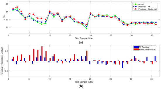
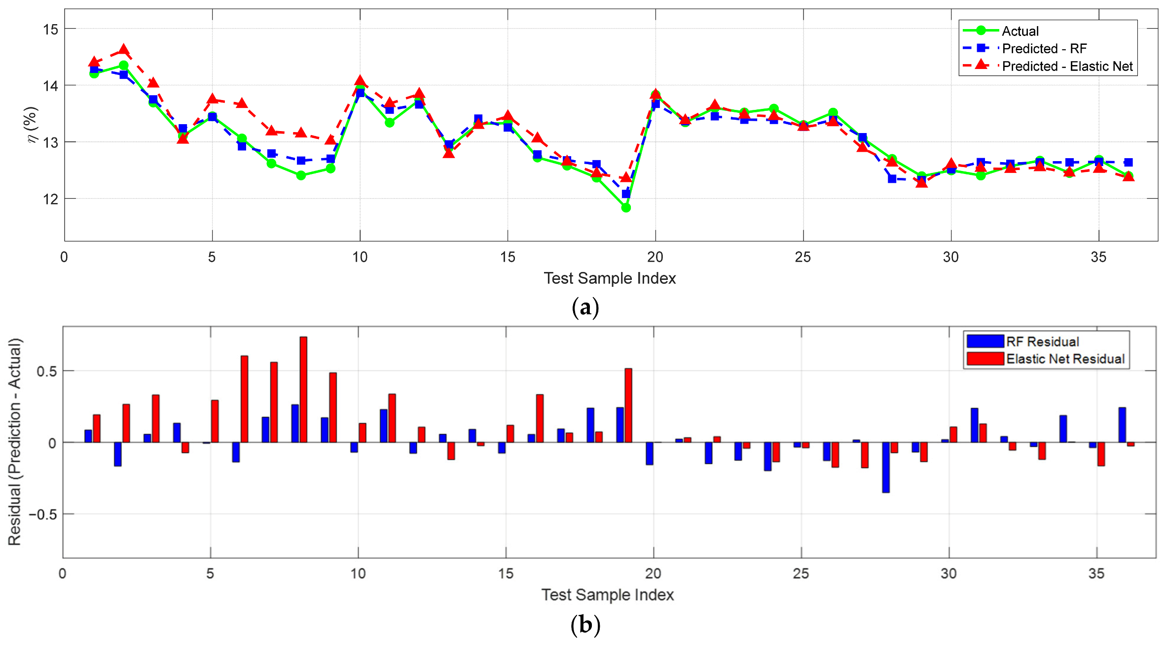
For completeness, Figure 5a shows the actual measured efficiency, η (in %), for each of the 36 independent test samples (green circles connected by a solid line), alongside the efficiencies predicted by two regression models: the RF predictor (blue squares, dashed line) and the EN predictor (red triangles, dashed line). Sample indices range from 1 to 36 on the horizontal axis, while the vertical axis displays efficiency values ranging from approximately 11.8% to 14.7%. Overall, both models capture the general trends in the experimental data, yet discrepancies are evident. In particular, the EN model systematically overpredicts the efficiencies for the first ten testing samples. By contrast, the RF predictions remain more tightly clustered around the measured values throughout the entire range of samples.

Figure 5. (a) The actual and estimated PV daily system conversion efficiency obtained by the RF and EN prediction models for the test dataset, (b) the residuals for prediction models at each sample index.

In Figure 5b, the residuals for each model are plotted as vertical bars at each sample index: RF residuals in blue and EN residuals in red. The residual is defined as the estimated efficiency ($\widehat{\eta }$) minus the actual measured efficiency ($\eta$), so positive bars indicate overprediction and negative bars indicate underprediction. The RF residuals remain small in magnitude (approximately ±0.3 %), with no apparent systematic bias, demonstrating tightly centered, zero-mean errors. By contrast, the EN residuals exhibit a clear positive bias for the first ten samples—peaking at around +0.7 % for sample 8—and remain larger in variance throughout. Between samples 20 and 30, both models slightly underpredict efficiency (negative residuals), but the RF underprediction is limited to approximately –0.2%, whereas EN again displays larger deviations (up to –0.3%). Across the 36 test samples, RF consistently shows the fewest errors in nearly two-thirds of the samples.

These residual patterns have a physical significance. Elastic Net applies a joint L1/L2 penalty to an essentially linear model and over-regularizes in small samples, failing to reproduce the mild curvature of the D-T-eta relationship. Its overprediction over the first ten test samples coincides with the post-cleaning regime, where efficiency is the highest and drops steeply as dust re-accumulates; the linear model lags a non-linear transient, so it overshoots. The tree- and kernel-based models represent this curvature and are, thus, the most different from EN in these transition regions, with the models coming together in the flatter high-dust regime later in each cycle.

6. Conclusions and Future Works

The high penetration of photovoltaic (PV) systems in electrical grids requires accurate prediction of their performance. Statistical and physical models may be used. But they may not be able to learn the complexity of the input–output relationship. In addition, the computational effort and cost can be enormous. Therefore, the previous constraints can be removed by employing Artificial Intelligence (AI) and machine learning (ML) models that can forecast the performance of complex PV systems with high accuracy and with less computational time and cost. In this paper, six proposed AI and ML models are tested to predict the performance of a 7.98 kWp on-grid PV system in Jordan and benchmarked against statistical models discussed in our previous works. The models proposed in this work are Decision Tree (DT), Random Forest (RF), Support Vector Machine (SVM), Gradient Boosting (GB), Gaussian Process Regression (GPR) and Elastic Net (EN). However, the benchmark models in our previous works are two Artificial Neural Network (ANN) variants, Extreme Learning Machine (ELM) and multiple linear regression (MLR), and conventional KNN and adaptive KNN.

Four performance metrics commonly employed in the literature are evaluated to assess the performance of the proposed and benchmark models. The metrics used for model comparison are Mean Square Error (MSE), accuracy, Coefficient of Determination (R²) and adjusted R² ($R_{adjusted}^2$). The results showed that some of the proposed models outperformed some benchmark models, while others outperformed some proposed models, indicating that no single class of model is universally better than another.

Based on the Decision Matrix, RF has performed better than all proposed and benchmark models overall. Simultaneously, EN is the worst prediction model among all 12 of the proposed and benchmark models discussed in this work. The remaining proposed models (GPR, SVM, DT and GB) showed intermediate predictive performance.

The proposed RF model outperforms the others for all four metrics with low error, high accuracy and good explanatory power. Models such as these are suitable candidates for PV efficiency prediction tasks. However, the proposed model (EN) performs poorly in all metrics and is consistently the least effective in this analysis. It may not have found a good fit for the current dataset given its linear assumptions or over-regularization. The other proposed models, such as GPR, SVM, DT, and GB, offer more balanced trade-offs and are appropriate when computational resources are limited or interpretability is not essential.

The comparative analysis indicates that the RF model performed the best on this dataset, suggesting that ensemble and non-linear methods can help on small PV datasets of this type. This means that RF’s high explanatory power and low error, consistent across the dataset, support its practical use for PV system performance prediction, despite its longer training time than simpler models.

6.1. Limitations

The results should be read within the scope of the case considered. The analysis is limited to a single 7.98 kWp rooftop system at a single site using 179 days of data from a single spring–summer period and two physically motivated inputs; performance at other capacities, dust intensities, climate zones, seasons, and richer input sets was not explored. As the two predictors evolve slowly over time, the random train/test split provides a fair basis for relative comparisons among models—all share the same split—but the absolute metric levels may be somewhat optimistic relative to a strictly chronological deployment. A blocked, leave-one-cleaning-cycle-out validation is identified below to quantify this. The deployment recommendations are, therefore, suggestive rather than conclusive and should be validated on other systems.

6.2. Future Work

There are several specific directions. First, the input space may be augmented with extra meteorological and soiling variables (e.g., humidity, wind, a measured soiling ratio). Secondly, hybrid physical machine learning models can embed the physics of temperature and soiling within a data-driven predictor. Third, the RF predictions can be used to optimize the PV cleaning schedule, balancing the predicted efficiency recovery and cleaning cost. Fourth, the framework can be extended from same-day estimation to multi-day-ahead time-series forecasting, with chronological, blocked, leave-one-cleaning-cycle-out validation. Finally, the models must be validated across multiple PV systems with varying capacities, dust intensities, climate zones, and seasons.

References

- Sobri, S.; Koohi-Kamali, S.; Rahim, N.A. Solar Photovoltaic Generation Forecasting Methods: A Review. Energy Convers. Manag. 2018, 156, 459–497. [Google Scholar] [CrossRef] [Scilit]
- Iheanetu, K.J. Solar Photovoltaic Power Forecasting: A Review. Sustainability 2022, 14, 17005. [Google Scholar] [CrossRef] [Scilit]
- Sharma, J.; Soni, S.; Paliwal, P.; Saboor, S.; Chaurasiya, P.K.; Sharifpur, M.; Khalilpoor, N.; Afzal, A. A Novel Long Term Solar Photovoltaic Power Forecasting Approach Using LSTM with Nadam Optimizer: A Case Study of India. Energy Sci. Eng. 2022, 10, 2909–2929. [Google Scholar] [CrossRef] [Scilit]
- Akhter, M.N.; Mekhilef, S.; Mokhlis, H.; Shah, N.M. Review on Forecasting of Photovoltaic Power Generation Based on Machine Learning and Metaheuristic Techniques. IET Renew. Power Gener. 2019, 13, 1009–1023. [Google Scholar] [CrossRef] [Scilit]
- Mellit, A.; Kalogirou, S.A. Artificial Intelligence Techniques for Photovoltaic Applications: A Review. Prog. Energy Combust. Sci. 2008, 34, 574–632. [Google Scholar] [CrossRef] [Scilit]
- Ramadhan, R.A.A.; Heatubun, Y.R.J.; Tan, S.F.; Lee, H.J. Comparison of Physical and Machine Learning Models for Estimating Solar Irradiance and Photovoltaic Power. Renew. Energy 2021, 178, 1006–1019. [Google Scholar] [CrossRef] [Scilit]
- Abdullah, A.S.; Joseph, A.; Kandeal, A.W.; Alawee, W.H.; Peng, G.; Thakur, A.K.; Sharshir, S.W. Application of Machine Learning Modeling in Prediction of Solar Still Performance: A Comprehensive Survey. Results Eng. 2024, 21, 101800. [Google Scholar] [CrossRef] [Scilit]
- Abubakar Mas’ud, A. Comparison of Three Machine Learning Models for the Prediction of Hourly PV Output Power in Saudi Arabia. Ain Shams Eng. J. 2022, 13, 101648. [Google Scholar] [CrossRef] [Scilit]
- Yılmaz, H.; Şahin, M. Solar Panel Energy Production Forecasting by Machine Learning Methods and Contribution of Lifespan to Sustainability. Int. J. Environ. Sci. Technol. 2023, 20, 10999–11018. [Google Scholar] [CrossRef] [Scilit]
- Long, H.; Zhang, Z.; Su, Y. Analysis of Daily Solar Power Prediction with Data-Driven Approaches. Appl. Energy 2014, 126, 29–37. [Google Scholar] [CrossRef] [Scilit]
- Wang, F.; Zhen, Z.; Wang, B.; Mi, Z. Comparative Study on KNN and SVM Based Weather Classification Models for Day Ahead Short Term Solar PV Power Forecasting. Appl. Sci. 2017, 8, 28. [Google Scholar] [CrossRef] [Scilit]
- Kassim, N.M.; Santhiran, S.; Alkahtani, A.A.; Islam, M.A.; Tiong, S.K.; Mohd Yusof, M.Y.; Amin, N. An Adaptive Decision Tree Regression Modeling for the Output Power of Large-Scale Solar (LSS) Farm Forecasting. Sustainability 2023, 15, 13521. [Google Scholar] [CrossRef] [Scilit]
- Jumin, E.; Basaruddin, F.B.; Yusoff, Y.B.M.; Latif, S.D.; Ahmed, A.N. Solar Radiation Prediction Using Boosted Decision Tree Regression Model: A Case Study in Malaysia. Environ. Sci. Pollut. Res. 2021, 28, 26571–26583. [Google Scholar] [CrossRef] [Scilit] [PubMed]
- Tato, J.H.; Brito, M.C. Using Smart Persistence and Random Forests to Predict Photovoltaic Energy Production. Energies 2019, 12, 100. [Google Scholar] [CrossRef] [Scilit]
- Lahouar, A.; Mejri, A.; Ben Hadj Slama, J. Importance Based Selection Method for Day-Ahead Photovoltaic Power Forecast Using Random Forests. In Proceedings of the 2017 International Conference on Green Energy and Conversion Systems; GECS 2017; IEEE: New York, NY, USA, 2017. [Google Scholar]
- Ahmad, A.; Jin, Y.; Zhu, C.; Javed, I.; Waqar Akram, M.; Buttar, N.A. Support Vector Machine Based Prediction of Photovoltaic Module and Power Station Parameters. Int. J. Green Energy 2020, 17, 219–232. [Google Scholar] [CrossRef] [Scilit]
- Mahesh, P.V.; Meyyappan, S.; Alia, R.K.R. Support Vector Regression Machine Learning Based Maximum Power Point Tracking for Solar Photovoltaic Systems. Int. J. Electr. Comput. Eng. Syst. 2023, 14, 100–108. [Google Scholar] [CrossRef] [Scilit]
- Polo, J.; Martín-Chivelet, N.; Alonso-Abella, M.; Sanz-Saiz, C.; Cuenca, J.; de la Cruz, M. Exploring the PV Power Forecasting at Building Façades Using Gradient Boosting Methods. Energies 2023, 16, 1495. [Google Scholar] [CrossRef] [Scilit]
- Rinesh, S.S.; Deepa, R.T.; Nandan, R.S.; Sachin, S.V.; Thamil, R.; Akash, M.; Prajitha, C.; Senthil Kumar, A.P. Prediction and Classification of Solar Photovoltaic Power Generation Using Extreme Gradient Boosting Regression Model. Int. J. Low-Carbon Technol. 2024, 19, 2420–2430. [Google Scholar] [CrossRef] [Scilit]
- Islam, M.S.S.; Ghosh, P.; Faruque, M.O.; Islam, M.R.; Hossain, M.A.; Alam, M.S.; Islam Sheikh, M.R. Optimizing Short-Term Photovoltaic Power Forecasting: A Novel Approach with Gaussian Process Regression and Bayesian Hyperparameter Tuning. Processes 2024, 12, 546. [Google Scholar] [CrossRef] [Scilit]
- Achouri, F.; Damou, M.; Harrou, F.; Sun, Y.; Bouyeddou, B. Gaussian Processes for Efficient Photovoltaic Power Prediction. In Proceedings of the 2023 International Conference on Decision Aid Sciences and Applications; DASA 2023; IEEE: New York, NY, USA, 2023. [Google Scholar]
- Yaghoubi, A.A.; Gandomzadeh, M.; Gholami, A.; Gavagsaz-Ghoachani, R.; Zandi, M.; Phattanasak, M. Harnessing Machine Learning with Advanced Linear Regression Models to Forecast PV System. In Proceedings of the 2024 International Conference on Materials and Energy: Energy in Electrical Engineering (ICOME-EE), Bangkok, Thailand, 30 October–1 November 2024; IEEE: New York, NY, USA, 2024; pp. 1–4. [Google Scholar]
- Mohanasundaram, V.; Rangaswamy, B. Elastic Net with Bayesian Density Estimation Model for Feature Selection for Photovoltaic Energy Prediction. Sci. Rep. 2025, 15, 8736. [Google Scholar] [CrossRef] [Scilit] [PubMed]
- Hammad, B.; Al-Abed, M.; Al-Ghandoor, A.; Al-Sardeah, A.; Al-Bashir, A. Modeling and Analysis of Dust and Temperature Effects on Photovoltaic Systems’ Performance and Optimal Cleaning Frequency: Jordan Case Study. Renew. Sustain. Energy Rev. 2018, 82, 2218–2234. [Google Scholar] [CrossRef] [Scilit]
- Al-Kouz, W.; Al-Dahidi, S.; Hammad, B.; Al-Abed, M. Modeling and Analysis Framework for Investigating the Impact of Dust and Temperature on PV Systems’ Performance and Optimum Cleaning Frequency. Appl. Sci. 2019, 9, 1397. [Google Scholar] [CrossRef] [Scilit]
- Al-Dahidi, S.; Hammad, B.; Alrbai, M.; Al-Abed, M. A Novel Dynamic/Adaptive K-Nearest Neighbor Model for the Prediction of Solar Photovoltaic Systems’ Performance. Results Eng. 2024, 22, 102141. [Google Scholar] [CrossRef] [Scilit]
- Rahman, T.; Mansur, A.A.; Hossain Lipu, M.S.; Rahman, M.S.; Ashique, R.H.; Houran, M.A.; Elavarasan, R.M.; Hossain, E. Investigation of Degradation of Solar Photovoltaics: A Review of Aging Factors, Impacts, and Future Directions toward Sustainable Energy Management. Energies 2023, 16, 3706. [Google Scholar] [CrossRef] [Scilit]
- Shenouda, R.; Abd-Elhady, M.S.; Kandil, H.A. A Review of Dust Accumulation on PV Panels in the MENA and the Far East Regions. J. Eng. Appl. Sci. 2022, 69, 8. [Google Scholar] [CrossRef] [Scilit]
- Hammad, B.K.; Rababeh, S.M.; Al-Abed, M.A.; Al-Ghandoor, A.M. Performance Study of On-Grid Thin-Film Photovoltaic Solar Station as a Pilot Project for Architectural Use. Jordan J. Mech. Ind. Eng. 2013, 7, 1–9. [Google Scholar]
- Mienye, I.D.; Jere, N. A Survey of Decision Trees: Concepts, Algorithms, and Applications. IEEE Access 2024, 12, 86716–86727. [Google Scholar] [CrossRef] [Scilit]
- Priyanka; Kumar, D. Decision Tree Classifier: A Detailed Survey. Int. J. Inf. Decis. Sci. 2020, 12, 246. [Google Scholar] [CrossRef] [Scilit]
- Močkus, J. On Bayesian Methods for Seeking the Extremum. In Proceedings of the Optimization Techniques IFIP Technical Conference, Novosibirsk, Russia, 1–7 July 1974; Springer: Berlin/Heidelberg, Germany, 1975; pp. 400–404. [Google Scholar]
- Salman, H.A.; Kalakech, A.; Steiti, A. Random Forest Algorithm Overview. Babylon. J. Mach. Learn. 2024, 2024, 69–79. [Google Scholar] [CrossRef] [Scilit] [PubMed]
- Wu, J.; Chen, X.Y.; Zhang, H.; Xiong, L.D.; Lei, H.; Deng, S.H. Hyperparameter Optimization for Machine Learning Models Based on Bayesian Optimization. J. Electron. Sci. Technol. 2019, 17, 26–40. [Google Scholar] [CrossRef]
- Tian, Y.; Shi, Y.; Liu, X. Recent Advances on Support Vector Machines Research. Technol. Econ. Dev. Econ. 2012, 18, 5–33. [Google Scholar] [CrossRef] [Scilit]
- Wang, D.; Wang, C.; Xiao, J.; Xiao, Z.; Chen, W.; Havyarimana, V. Bayesian Optimization of Support Vector Machine for Regression Prediction of Short-Term Traffic Flow. Intell. Data Anal. 2019, 23, 481–497. [Google Scholar] [CrossRef] [Scilit]
- Sibindi, R.; Mwangi, R.W.; Waititu, A.G. A Boosting Ensemble Learning Based Hybrid Light Gradient Boosting Machine and Extreme Gradient Boosting Model for Predicting House Prices. Eng. Rep. 2023, 5, e12599. [Google Scholar] [CrossRef] [Scilit]
- Friedman, J.H. Greedy Function Approximation: A Gradient Boosting Machine. Ann. Stat. 2001, 29, 1189–1232. [Google Scholar] [CrossRef] [Scilit]
- Seeger, M. Gaussian Processes for Machine Learning. Int. J. Neural Syst. 2004, 14, 69–106. [Google Scholar] [CrossRef] [Scilit] [PubMed]
- Bharti; Naheliya, B.; Kumar, K. Short-Term Traffic Flow Prediction in Heterogeneous Traffic Conditions Using Gaussian Process Regression. Int. J. Inf. Technol. 2024, 17, 5661–5671. [Google Scholar] [CrossRef] [Scilit]
- Zou, H.; Hastie, T. Regularization and Variable Selection via the Elastic Net. J. R. Stat. Soc. Ser. B Stat. Methodol. 2005, 67, 301–320. [Google Scholar] [CrossRef] [Scilit]
Disclaimer/Publisher’s Note: The statements, opinions and data contained in all publications are solely those of the individual author(s) and contributor(s) and not of MDPI and/or the editor(s). MDPI and/or the editor(s) disclaim responsibility for any injury to people or property resulting from any ideas, methods, instructions or products referred to in the content. |
© 2026 by the authors. Licensee MDPI, Basel, Switzerland. This article is an open access article distributed under the terms and conditions of the Creative Commons Attribution (CC BY) license.