Periodic Orbits and KAM Tori in the Hénon–Heiles Hamiltonian System: The 1: ω Resonance Case

Abstract

We prove the existence and determine the linear stability of periodic orbits in the Hénon–Heiles Hamiltonian system under a $1:\omega$ resonance, with $\omega \ge 2$. The analysis combines Lie–Deprit normalization with regular and singular reduction. We also establish the persistence of two-dimensional KAM tori surrounding the linearly stable periodic orbits and derive periodic asymptotic parametrizations in the original variables.

1. Introduction

The Hénon–Heiles system is one of the paradigmatic models in nonlinear Hamiltonian dynamics. Originally introduced in galactic dynamics in connection with the search for a third integral of motion [1], it has become a classical framework for studying resonances, integrability, and chaotic behavior in Hamiltonian systems. Hénon–Heiles Hamiltonians and their generalizations have been extensively used to analyze periodic orbits, bifurcations, stability transitions, and the coexistence of regular and chaotic regions in phase space [2,3,4,5].

From the point of view of integrability, Hénon–Heiles-type Hamiltonians exhibit a rich structure. Although some exceptional cases are Liouville-integrable, the generic case is nonintegrable and gives rise to complex dynamics [6,7,8]. Further results on integrability, completeness, and separability for cubic and quartic Hénon–Heiles Hamiltonians can be found, for instance, in [9,10].

A relevant family of generalized Hénon–Heiles Hamiltonians is given by

$$\mathcal{H}(x,y)={\displaystyle \frac{1}{2}}(y_1^2+y_2^2)+{\displaystyle \frac{1}{2}}({\omega }_1^2{x}_1^2+{\omega }_2^2{x}_2^2)+a{x}_1^2{x}_2+b{x}_2^3,$$

(1)

where $a,b\in \mathbb{R}$ and ${\omega }_1,{\omega }_2>0$. The classical Hénon–Heiles Hamiltonian is recovered by taking ${\omega }_1={\omega }_2=1$ and $b=-a/3$. Special choices of the parameters lead to distinguished integrable cases. These include the Sawada–Kotera case, $b=a/3$ with ${\omega }_2={\omega }_1$, corresponding to the $1:1$ resonance; the Korteweg–de Vries case, $b=2a$, whose subcase ${\omega }_2=2{\omega }_1$ corresponds to the $1:2$ resonance; and the Kaup–Kupershmidt case, $b=16a/3$ with ${\omega }_2=4{\omega }_1$, corresponding to the $1:4$ resonance [7,9,10,11].

Motivated by this framework, we consider the perturbed Hamiltonian

$${\mathcal{H}}_{\epsilon }(x,y)={\displaystyle \frac{1}{2}}(y_1^2+y_2^2)+{\displaystyle \frac{1}{2}}({\omega }_1^2{x}_1^2+{\omega }_2^2{x}_2^2)+\epsilon \left(a{x}_1^2{x}_2+b{x}_2^3\right),$$

(2)

where $\epsilon$ is a small real parameter. After the linear symplectic scaling

$$x_i\mapsto {\displaystyle \frac{x_i}{\sqrt{{\omega }_i}}}, y_i\mapsto \sqrt{{\omega }_i}{y}_i,i=1,2,$$

and the time rescaling $t\mapsto t/{\omega }_1$, Hamiltonian (2) becomes

$${\mathcal{H}}_{\epsilon }(x,y)={\displaystyle \frac{1}{2}}(x_1^2+y_1^2)+{\displaystyle \frac{\omega }{2}}(x_2^2+y_2^2)+\epsilon \left(\alpha x_1^2{x}_2+\beta x_2^3\right),$$

(3)

where

$$\omega ={\displaystyle \frac{{\omega }_2}{{\omega }_1}},\alpha ={\displaystyle \frac{a}{{\omega }_1^2\sqrt{\omega {\omega }_1}}},\beta ={\displaystyle \frac{b}{\omega {\omega }_1^2\sqrt{\omega {\omega }_1}}}.$$

Throughout this work, we assume that

$${\displaystyle \frac{{\omega }_2}{{\omega }_1}}=\omega \in \mathbb{N}.$$

The unperturbed part of (3) is

$${\mathcal{H}}_0(x,y)={\displaystyle \frac{1}{2}}(x_1^2+y_1^2)+{\displaystyle \frac{\omega }{2}}(x_2^2+y_2^2),$$

which defines an anisotropic harmonic oscillator in $1:\omega$ resonance. Thus, the Hamiltonian (3) is a Hénon–Heiles-type perturbation of this integrable resonant oscillator.

The isotropic case $\omega =1$ has been studied in connection with periodic orbits, integrability, and bifurcations; see, for instance, [4,7,12]. We therefore focus on the anisotropic resonant case $\omega \ge 2$.

Hamiltonians of the form (3) arise naturally in the study of resonant periodic motions and invariant structures near elliptic equilibria. In this setting, reduction, averaging, and normal form methods provide effective tools for detecting periodic orbits and for analyzing their bifurcations and linear stability [13,14,15,16]. Moreover, normal form techniques provide accurate local models for the regular regime of the dynamics, the persistence of invariant structures, and the transition to chaos in generalized Hénon–Heiles Hamiltonians [5,17]. The persistence of quasi-periodic invariant tori is obtained by applying the higher-order properly degenerate KAM theorem of Han, Li, and Yi both in the $1:2$ case and for the higher resonances with $\omega \ge 3$ [18].

Works [19,20] develop geometric averaging methods for periodic solutions and their stability, including KAM persistence, whereas [16] develops singular reduction for resonant Hamiltonian systems. In the Hénon–Heiles setting, ref. [15] applies Reeb’s theorem to study periodic orbits in a rotating potential. Building on these results, we give a unified analysis of Hamiltonian (3) for every integer $1:\omega$ resonance with $\omega \ge 2$. Our contribution combines the separate treatment of the cubic $1:2$ resonance and the higher-order resonances with $\omega \ge 3$, the reconstruction of periodic orbits from both regular and singular critical points, their linear stability classification, the persistence of surrounding KAM tori, and periodic asymptotic parametrizations in the original variables.

The paper is organized as follows. In Section 2, we introduce the polynomial invariants associated with ${\mathcal{H}}_0$, compute the normal form of Hamiltonian (3) using the Lie–Deprit method, and express the reduced Hamiltonian in terms of these invariants. We also determine the corresponding Poisson structure and characterize the critical points of the reduced system. In Section 3, we construct symplectic coordinates $(L,Q,\ell ,P)$ adapted to the $1:\omega$ resonance and derive explicit relations between these coordinates and the polynomial invariants describing the reduced space. In Section 4, we reconstruct periodic orbits from the critical points by applying Reeb’s theorem and singular reduction results, and we determine their linear stability or instability using parametric stability criteria [21,22]. We also prove the persistence of two-dimensional invariant tori around the linearly stable periodic orbits. In Section 5, we derive and verify periodic asymptotic parametrizations in the original variables, compare them with direct numerical integrations, and illustrate the nearby KAM structure by means of Poincaré sections. Section 6 summarizes the main results and outlines directions for future research. Finally, the collects the main tools used throughout the paper, including Reeb-type results for resonant Hamiltonian systems and KAM results for degenerate Hamiltonian systems.

2. Reduction and Normalization

To describe the orbit space associated with the unperturbed Hamiltonian ${\mathcal{H}}_0$, we identify ${\mathbb{R}}^4$ with ${\mathbb{C}}^2$ through the complex coordinates ${\zeta }_1=x_1+i{y}_1$ and ${\zeta }_2=x_2+i{y}_2$. In these variables,

$${\mathcal{H}}_0={\displaystyle \frac{1}{2}}\left(|{\zeta }_1{|}^2+\omega {\left|{\zeta }_2\right|}^2\right),$$

(4)

and the Hamiltonian flow of ${\mathcal{H}}_0$ generates the $S^1$-action $\phi :S^1\times {\mathbb{C}}^2\to {\mathbb{C}}^2$ given by

$$\phi (t,\zeta )=\left(e^{-it}{\zeta }_1,e^{-i\omega t}{\zeta }_2\right).$$

This action is proper. For every $h>0$, its restriction to the energy level ${\mathcal{N}}_0\left(h\right)={\mathcal{H}}_0^{-1}\left(h\right)$ is free when $\omega =1$ and locally free when $\omega \ge 2$. Consequently, the quotient

$$\mathcal{B}\left(h\right)={\mathcal{N}}_0\left(h\right)/S^1$$

is a compact symplectic manifold for $\omega =1$ and a compact symplectic orbifold for $\omega \ge 2$. This quotient is the reduced space associated with the resonant $S^1$-action; see, for example, [16,23,24].

Since

$${\mathcal{N}}_0\left(h\right)=\{\zeta \in {\mathbb{C}}^2:|{\zeta }_1{|}^2+\omega |{\zeta }_2{|}^2=2h\}$$

is a three-dimensional manifold, the reduced space $\mathcal{B}\left(h\right)$ has dimension two. For $\omega =1$, it is diffeomorphic to ${\mathbb{CP}}^1$, whereas for $\omega \ge 2$ it can be naturally realized as a weighted projective space with a singular point corresponding to the second normal mode.

The reduced space can be described in terms of polynomial invariants of the $1:\omega$ resonant oscillator. We denote these invariants by ${\pi }_1,{\pi }_2,{\pi }_3,{\pi }_4$. They are first integrals of ${\mathcal{H}}_0$, that is,

$$\{{\mathcal{H}}_0,{\pi }_j\}=0,j=1,2,3,4,$$

and generate the algebra of polynomial invariants associated with the induced $S^1$-action; see [16,25]. Explicitly,

$$\begin{array}{cccccc}\hfill {\pi }_1& =& x_1^2+y_1^2,\hfill & \hfill {\pi }_2& =& x_2^2+y_2^2,\hfill \\ \hfill {\pi }_3& =& Re\left[{(x_1-i{y}_1)}^{\omega }(x_2+i{y}_2)\right],\hfill & \hfill {\pi }_4& =& Im\left[{(x_1-i{y}_1)}^{\omega }(x_2+i{y}_2)\right].\hfill \end{array}$$

(5)

These invariants satisfy the algebraic relations

$${\pi }_3^2+{\pi }_4^2={\pi }_1^{\omega }{\pi }_2,{\pi }_1+\omega {\pi }_2=2{\mathcal{H}}_0,$$

(6)

together with

$${\pi }_1\ge 0,{\pi }_2\ge 0.$$

(7)

Table 1 displays the Poisson structure induced by the invariants, which is obtained by a direct computation of their standard Poisson brackets.

Table 1. Poisson brackets among the invariants ${\pi }_1,\dots ,{\pi }_4$.

$\left\{{\mathit{\pi }}_{\mathit{j}},{\mathit{\pi }}_{\mathit{k}}\right\}$	${\mathit{\pi }}_1$	${\mathit{\pi }}_2$	${\mathit{\pi }}_3$	${\mathit{\pi }}_4$
${\pi }_1$	0	0	$2\omega {\pi }_4$	$-2\omega {\pi }_3$
${\pi }_2$	0	0	$-2{\pi }_4$	$2{\pi }_3$
${\pi }_3$	$-2\omega {\pi }_4$	$2{\pi }_4$	0	${\pi }_1^{\omega -1}({\pi }_1-{\omega }^2{\pi }_2)$
${\pi }_4$	$2\omega {\pi }_3$	$-2{\pi }_3$	$-{\pi }_1^{\omega -1}({\pi }_1-{\omega }^2{\pi }_2)$	0

This Poisson structure will be used below to write the reduced Hamiltonian in invariant coordinates.

We exploit the resonant symmetry of the anisotropic oscillator by applying the Lie–Deprit normalization method to Hamiltonian (3) [13,14]. The first nonzero resonant terms depend on the resonance order: for $\omega =2$, cubic resonant terms appear at order $\epsilon$; for $\omega \ge 3$, all cubic terms are nonresonant and can be removed, so the first effective contribution appears at order ${\epsilon }^2$ and has degree four.

For completeness, we specify the Lie–Deprit normalization conventions used below; see [14,21]. Set $z=(x,y)$, $Z=(X,Y),$ and denote the cubic perturbation in (3) by

$${\mathcal{P}}_3\left(z\right)=\alpha x_1^2{x}_2+\beta x_2^3,{\mathcal{H}}_{\epsilon }\left(z\right)={\mathcal{H}}_0\left(z\right)+\epsilon {\mathcal{P}}_3\left(z\right).$$

We use the convention ${\mathcal{L}}_g\left(f\right)=\left\{f,g\right\}$ and the generating function

$$W(\epsilon ,z)={\displaystyle \sum _{j=0}^{\infty }}{\displaystyle \frac{{\epsilon }^j}{j!}}{W}_{j+1}\left(z\right)=W_1\left(z\right)+\epsilon W_2\left(z\right)+\dots ,$$

where each $W_j$ is a homogeneous polynomial of degree $j+2$ in z. The associated near-identity symplectic transformation $z=z(\epsilon ,Z)$ is generated by

$${\displaystyle \frac{\partial z}{\partial \epsilon }}(\epsilon ,Z)=\mathbb{J}\nabla W\left(\epsilon ,z(\epsilon ,Z)\right),z(0,Z)=Z,$$

where $\mathbb{J}$ is the standard symplectic matrix.

Writing the transformed Hamiltonian as

$${\mathcal{H}}_{\epsilon }^N={\mathcal{H}}_0+\epsilon {\mathcal{H}}_1+{\epsilon }^2{\mathcal{H}}_2+O\left({\epsilon }^3\right),$$

the first two rows of the Lie–Deprit triangle yield the homological equations

$${\mathcal{H}}_1={\mathcal{P}}_3+\left\{{\mathcal{H}}_0,W_1\right\},2{\mathcal{H}}_2=\left\{{\mathcal{P}}_3,W_1\right\}+\left\{{\mathcal{H}}_0,W_2\right\}+\left\{{\mathcal{H}}_1,W_1\right\}.$$

At each order, $W_j$ is chosen so that the corresponding normal-form term satisfies

$$\left\{{\mathcal{H}}_0,{\mathcal{H}}_j\right\}=0.$$

For $\omega =2$, the resonant cubic term ${\mathcal{H}}_1$ is nonzero. For $\omega \ge 3$, all cubic terms are nonresonant, so ${\mathcal{H}}_1=0$, and the second homological equation reduces to

$${\mathcal{H}}_2={\displaystyle \frac{1}{2}}\left(\left\{{\mathcal{P}}_3,W_1\right\}+\left\{{\mathcal{H}}_0,W_2\right\}\right).$$

After computing the normal form, we relabel Z as z and ${\mathcal{H}}_{\epsilon }^N$ as ${\mathcal{H}}_{\epsilon }$.

For $\omega =2$, the normal form of Hamiltonian (3) contains resonant cubic terms and is given by

$${\mathcal{H}}_{\epsilon }(x,y)={\displaystyle \frac{1}{2}}(x_1^2+y_1^2)+x_2^2+y_2^2+\epsilon {\mathcal{H}}_1(x,y)+O\left({\epsilon }^2\right),$$

(8)

where

$${\mathcal{H}}_1(x,y)={\displaystyle \frac{\alpha }{4}}(2x_1{y}_1{y}_2+x_1^2{x}_2-x_2{y}_1^2).$$

This normal form is obtained, up to the first order, from the symplectic near-identity transformation

$$(x,y)=(X,Y)+\epsilon {\mathcal{L}}_{W_1}(X,Y)+O\left({\epsilon }^2\right),$$

(9)

where ${\mathcal{L}}_{W_1}(X,Y)=\mathbb{J}\nabla W_1(X,Y)$, and

$$W_1=-{\displaystyle \frac{\alpha }{16}}(2x_1{x}_2{y}_1+5x_1^2{y}_2+3y_1^2{y}_2)-{\displaystyle \frac{\beta }{6}}{y}_2(3x_2^2+2y_2^2).$$

Thus, Hamiltonian (8) can be written in invariant coordinates as

$${\mathcal{H}}_{\epsilon }\left(\pi \right)={\displaystyle \frac{1}{2}}({\pi }_1+2{\pi }_2)+\epsilon \left({\displaystyle \frac{\alpha }{4}}{\pi }_3\right)+O\left({\epsilon }^2\right).$$

(10)

For $\omega \ge 3$, the normalized Hamiltonian contains terms of degree four at order ${\epsilon }^2$ and is given by

$${\mathcal{H}}_{\epsilon }(x,y)={\displaystyle \frac{1}{2}}(x_1^2+y_1^2)+{\displaystyle \frac{\omega }{2}}(x_2^2+y_2^2)+{\epsilon }^2{\mathcal{H}}_2(x,y)+O\left({\epsilon }^3\right),$$

(11)

where

$${\mathcal{H}}_2(x,y)=\gamma {(x_1^2+y_1^2)}^2+\delta (x_1^2+y_1^2)(x_2^2+y_2^2)+\mu {(x_2^2+y_2^2)}^2$$

with

$$\gamma ={\displaystyle \frac{{\alpha }^2(8-3{\omega }^2)}{16\omega ({\omega }^2-4)}},\delta ={\displaystyle \frac{\alpha (12\beta +2\alpha \omega -3\beta {\omega }^2)}{4\omega ({\omega }^2-4)}},\mu =-{\displaystyle \frac{15{\beta }^2}{16\omega }}.$$

Note that $\gamma \le 0$ and $\mu \le 0$ for $\omega \ge 3$; these inequalities are strict when $\alpha \ne 0$ and $\beta \ne 0$, respectively.

The normal form (11) is obtained, up to the second order, from the symplectic near-identity transformation

$$(x,y)=(X,Y)+\epsilon {\mathcal{L}}_{W_1}(X,Y)+{\displaystyle \frac{{\epsilon }^2}{2}}\left({\mathcal{L}}_{W_1}^2+{\mathcal{L}}_{W_2}\right)(X,Y)+O\left({\epsilon }^3\right),$$

(12)

where

$$\begin{array}{cc}\hfill W_1(x,y)=& {\displaystyle \frac{\alpha }{\omega ({\omega }^2-4)}}\left[(2-{\omega }^2)x_1^2{y}_2+2\omega x_1{x}_2{y}_1+2y_1^2{y}_2\right]-{\displaystyle \frac{\beta }{3\omega }}(3x_2^2{y}_2+2y_2^3),\hfill \\ \hfill W_2(x,y)=& {\displaystyle \frac{{\alpha }^2}{8\omega ({\omega }^2-4)}}{x}_1{y}_1\left[(5{\omega }^2-8)x_1^2+(3{\omega }^2-8)y_1^2\right]\hfill \\ \hfill & +{\displaystyle \frac{\alpha (4\beta -2\alpha \omega -3\beta {\omega }^2-4\alpha {\omega }^3+2\beta {\omega }^4)}{2{\omega }^2({\omega }^2-1)({\omega }^2-4)}}{x}_1^2{x}_2{y}_2\hfill \\ \hfill & +{\displaystyle \frac{\alpha (4\beta +8\alpha \omega -10\beta {\omega }^2-2\alpha {\omega }^3+3\beta {\omega }^4)}{2\omega ({\omega }^2-1)({\omega }^2-4)}}{x}_1{x}_2^2{y}_1\hfill \\ \hfill & +{\displaystyle \frac{\alpha (8\beta -4\alpha \omega -8\beta {\omega }^2-2\alpha {\omega }^3+3\beta {\omega }^4)}{2\omega ({\omega }^2-1)({\omega }^2-4)}}{x}_1{y}_1{y}_2^2\hfill \\ \hfill & +{\displaystyle \frac{\alpha (4\beta +6\alpha \omega -7\beta {\omega }^2)}{2{\omega }^2({\omega }^2-1)({\omega }^2-4)}}{x}_2{y}_1^2{y}_2+{\displaystyle \frac{3{\beta }^2}{8{\omega }^2}}{x}_2{y}_2(3x_2^2+5y_2^2).\hfill \end{array}$$

In terms of the invariants, Hamiltonian (11) can be written as

$${\mathcal{H}}_{\epsilon }\left(\pi \right)={\displaystyle \frac{1}{2}}({\pi }_1+\omega {\pi }_2)+{\epsilon }^2\left(\gamma {\pi }_1^2+\delta {\pi }_1{\pi }_2+\mu {\pi }_2^2\right)+O\left({\epsilon }^3\right).$$

(13)

The reduction is carried out by introducing the Hilbert map ${\rho }_{\pi }:{\mathbb{R}}^4\to {\mathbb{R}}^4$, defined by ${\rho }_{\pi }(x_1,x_2,y_1,y_2)=({\pi }_1,{\pi }_2,{\pi }_3,{\pi }_4)$. The image of this map is the orbit space of the ${\mathcal{H}}_0$-action, and the image of ${\mathcal{N}}_0\left(h\right)$ under ${\rho }_{\pi }$ is the reduced space; that is, $\mathcal{B}\left(h\right)={\rho }_{\pi }\left({\mathcal{N}}_0\left(h\right)\right)$.

Consider the projection $\mathfrak{p}:{\mathbb{R}}^4\to {\mathbb{R}}^3$ defined by

$$\mathfrak{p}({\pi }_1,{\pi }_2,{\pi }_3,{\pi }_4)=({\pi }_1,{\pi }_3,{\pi }_4).$$

Using the constraints (6) and (7), the reduced space $\mathcal{B}\left(h\right)$ can be identified with the surface $\overline{\mathcal{B}}\left(h\right)=\mathfrak{p}\left(\mathcal{B}\left(h\right)\right)$; namely,

$$\overline{\mathcal{B}}\left(h\right)=\left\{({\pi }_1,{\pi }_3,{\pi }_4)\in {\mathbb{R}}^3:{\pi }_3^2+{\pi }_4^2={\pi }_1^{\omega }\left({\displaystyle \frac{2h-{\pi }_1}{\omega }}\right),0\le {\pi }_1\le 2h\right\}.$$

(14)

The reduced Hamiltonian is obtained from (10) and (13) by restricting the first nonconstant terms to the fixed energy surface ${\mathcal{H}}_0=h$. Thus,

$$\overline{\mathcal{H}}=\left\{\begin{array}{cc}{\displaystyle \frac{\alpha }{4}}{\pi }_3,\hfill & \mathrm{if}\omega =2,\hfill \\ \gamma {\pi }_1^2+\delta {\pi }_1{\pi }_2+\mu {\pi }_2^2,\hfill & \mathrm{if}\omega \ge 3.\hfill \end{array}\right.$$

To compute the vector field associated with $\overline{\mathcal{H}}$ in the coordinates $({\pi }_1,{\pi }_2,{\pi }_3,{\pi }_4)$, we use Table 1 together with the relations

$${\displaystyle \frac{d{\pi }_j}{dt}}=\{{\pi }_j,\overline{\mathcal{H}}\}={\displaystyle \sum _{k=1}^4}\left\{{\pi }_j,{\pi }_k\right\}{\displaystyle \frac{\partial \overline{\mathcal{H}}}{\partial {\pi }_k}},j=1,\dots ,4.$$

(15)

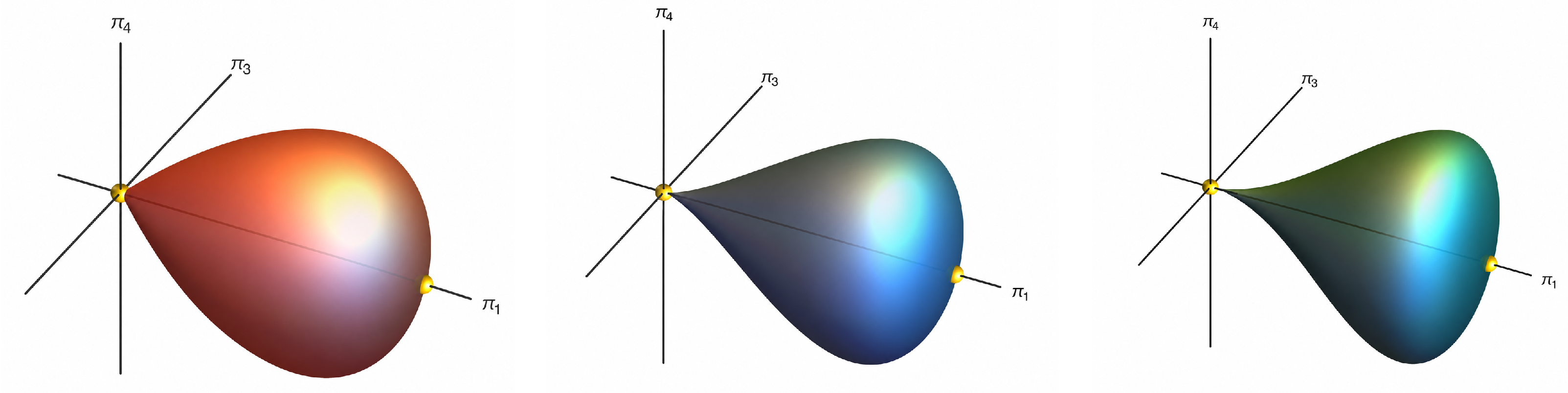
In the $1:\omega$ resonance, the reduced space $\mathcal{B}\left(h\right)$ has a singular point of peak-type at $\left(0,\frac{2h}{\omega },0,0\right)$, corresponding to the second normal mode of the unperturbed system. The remaining points of $\mathcal{B}\left(h\right)$ are regular and are called plateau points; see [16]. Denoting by ${\mathcal{O}}_0$ and ${\mathcal{O}}_1$ the points corresponding to the two normal modes, we obtain the following results.

Proposition 1.  

Assume that $\omega =2$ and $\alpha \ne 0$. On the reduced space $\mathcal{B}\left(h\right)$, the vector field (15) has three isolated critical points. One of them is the singular critical point ${\mathcal{O}}_0=(0,h,0,0)$, and the other two are the regular critical points

$${\mathcal{O}}_2=\left({\displaystyle \frac{4h}{3}},{\displaystyle \frac{h}{3}},{\displaystyle \frac{4h}{3}}\sqrt{{\displaystyle \frac{h}{3}}},0\right),{\mathcal{O}}_3=\left({\displaystyle \frac{4h}{3}},{\displaystyle \frac{h}{3}},-{\displaystyle \frac{4h}{3}}\sqrt{{\displaystyle \frac{h}{3}}},0\right).$$

Proof. 

For $\omega =2$, the reduced Hamiltonian obtained from (10) is

$$\overline{\mathcal{H}}={\displaystyle \frac{\alpha }{4}}{\pi }_3.$$

(16)

Using Table 1 and the relations (6), the critical points of the vector field (15) satisfy

$$\begin{array}{cc}\hfill {\pi }_4=& 0,\hfill \\ \hfill {\pi }_1({\pi }_1-4{\pi }_2)=& 0,\hfill \\ \hfill {\pi }_1+2{\pi }_2-2h=& 0,\hfill \\ \hfill {\pi }_3^2+{\pi }_4^2-{\pi }_1^2{\pi }_2=& 0.\hfill \end{array}$$

(17)

Solving system (17) gives the result. □

Remark 1.  

The critical point ${\mathcal{O}}_0=(0,h,0,0)$ corresponds to the singular point $(0,0,0)$ of the projected reduced space $\overline{\mathcal{B}}\left(h\right)$, shown in the left panel of Figure 1, whereas ${\mathcal{O}}_2$ and ${\mathcal{O}}_3$ correspond to regular points of this space.

Figure 1. Projected reduced spaces $\overline{\mathcal{B}}\left(h\right)$ in the coordinates $({\pi }_1,{\pi }_3,{\pi }_4)$ for a fixed energy $h>0$: $\omega =2$ (left), $\omega =3$ (middle), and $\omega =4$ (right). The highlighted points correspond to the two normal modes: the singular peak at ${\pi }_1=0$ and the endpoint at ${\pi }_1=2h$.

Proposition 2.  

Suppose that $\omega \ge 3$ and $(\alpha ,\beta )\ne (0,0)$. On the reduced space $\mathcal{B}\left(h\right)$, the system (15) always has the two critical points

$${\mathcal{O}}_0=\left(0,{\displaystyle \frac{2h}{\omega }},0,0\right),{\mathcal{O}}_1=(2h,0,0,0).$$

More precisely:

• If $(2\omega \gamma -\delta )(\omega \delta -2\mu )\ge 0$, then ${\mathcal{O}}_0$ and ${\mathcal{O}}_1$ are the only critical points.
• If $(2\omega \gamma -\delta )(\omega \delta -2\mu )<0$, then, in addition to ${\mathcal{O}}_0$ and ${\mathcal{O}}_1$, the system has a continuum of critical points of the form

  $$\left({\pi }_1^{*},{\displaystyle \frac{2h-{\pi }_1^{*}}{\omega }},{\pi }_3^{*},{\pi }_4^{*}\right)$$

  satisfying ${\left({\pi }_3^{*}\right)}^2+{\left({\pi }_4^{*}\right)}^2={\left({\pi }_1^{*}\right)}^{\omega }(2h-{\pi }_1^{*})/\omega$, where ${\pi }_1^{*}=\frac{(2\mu -\omega \delta )h}{{\omega }^2\gamma -\omega \delta +\mu }$.

Proof. 

For $\omega \ge 3$, the reduced Hamiltonian obtained from (13) is

$$\overline{\mathcal{H}}=\gamma {\pi }_1^2+\delta {\pi }_1{\pi }_2+\mu {\pi }_2^2.$$

(18)

Using Table 1 and the relations (6), the critical points of the vector field (15) in $\mathcal{B}\left(h\right)$ satisfy

$$\begin{array}{cc}\hfill {\pi }_3\left[(2\omega \gamma -\delta ){\pi }_1+(\omega \delta -2\mu ){\pi }_2\right]=& 0,\hfill \\ \hfill {\pi }_4\left[(2\omega \gamma -\delta ){\pi }_1+(\omega \delta -2\mu ){\pi }_2\right]=& 0,\hfill \\ \hfill {\pi }_1+\omega {\pi }_2-2h=& 0,\hfill \\ \hfill {\pi }_3^2+{\pi }_4^2-{\pi }_1^{\omega }{\pi }_2=& 0.\hfill \end{array}$$

(19)

The two coefficients appearing in the first two equations of (19) are

$$2\omega \gamma -\delta ={\displaystyle \frac{\alpha \left[\alpha \omega (4-3{\omega }^2)+6\beta ({\omega }^2-4)\right]}{8\omega ({\omega }^2-4)}}$$

and

$$\omega \delta -2\mu ={\displaystyle \frac{2\alpha \omega (12\beta +2\alpha \omega -3\beta {\omega }^2)+15{\beta }^2({\omega }^2-4)}{8\omega ({\omega }^2-4)}}.$$

For $\omega \ge 3$, a direct computation gives $(2\omega \gamma -\delta ,\omega \delta -2\mu )=(0,0)$ if and only if $(\alpha ,\beta )=(0,0)$. Hence, under the hypothesis $(\alpha ,\beta )\ne (0,0)$, these coefficients cannot vanish simultaneously. If $(2\omega \gamma -\delta )(\omega \delta -2\mu )\ge 0$, the first two equations in (19) imply that

$$(2\omega \gamma -\delta ){\pi }_1+(\omega \delta -2\mu ){\pi }_2=0$$

or ${\pi }_3={\pi }_4=0$. In the first case, since ${\pi }_1,{\pi }_2\ge 0$ and the two coefficients do not have opposite signs and cannot vanish simultaneously, we obtain ${\pi }_1{\pi }_2=0$. In the second case, the last equation in (19) gives the same conclusion. Thus, in both cases, ${\pi }_1{\pi }_2=0$ and ${\pi }_3={\pi }_4=0$. Using ${\pi }_1+\omega {\pi }_2=2h$, we obtain

$${\mathcal{O}}_0=\left(0,{\displaystyle \frac{2h}{\omega }},0,0\right),{\mathcal{O}}_1=(2h,0,0,0).$$

On the other hand, if $(2\omega \gamma -\delta )(\omega \delta -2\mu )<0$, then the factor $(2\omega \gamma -\delta ){\pi }_1+(\omega \delta -2\mu ){\pi }_2$ may vanish for points with $({\pi }_3,{\pi }_4)\ne (0,0)$. Thus, we solve the linear system

$$(2\omega \gamma -\delta ){\pi }_1+(\omega \delta -2\mu ){\pi }_2=0,{\pi }_1+\omega {\pi }_2=2h.$$

The determinant of its coefficient matrix is

$$\Delta =2({\omega }^2\gamma -\omega \delta +\mu )=-{\displaystyle \frac{3}{8\omega ({\omega }^2-4)}}\left[5({\omega }^2-4){\left(\beta -{\displaystyle \frac{2\omega }{5}}\alpha \right)}^2+{\displaystyle \frac{{\omega }^2({\omega }^2+16)}{5}}{\alpha }^2\right].$$

(20)

Since $\omega \ge 3$ and $(\alpha ,\beta )\ne (0,0)$, we have $\Delta <0$. Therefore, we obtain

$${\pi }_1^{*}={\displaystyle \frac{(2\mu -\omega \delta )h}{{\omega }^2\gamma -\omega \delta +\mu }},{\pi }_2^{*}={\displaystyle \frac{2h-{\pi }_1^{*}}{\omega }}.$$

Finally, the relation defining $\mathcal{B}\left(h\right)$ gives

$${\left({\pi }_3^{*}\right)}^2+{\left({\pi }_4^{*}\right)}^2={\left({\pi }_1^{*}\right)}^{\omega }{\pi }_2^{*}={\displaystyle \frac{1}{\omega }}{\left({\pi }_1^{*}\right)}^{\omega }(2h-{\pi }_1^{*}).$$

This proves the result. □

Remark 2.  

On the level surface ${\mathcal{N}}_0\left(h\right)={\mathcal{H}}_0^{-1}\left(h\right)$, the critical points obtained in Propositions 1 and 2 correspond to periodic orbits of the unperturbed Hamiltonian

$${\mathcal{H}}_0(x,y)={\displaystyle \frac{1}{2}}(x_1^2+y_1^2)+{\displaystyle \frac{\omega }{2}}(x_2^2+y_2^2).$$

Regular critical points correspond to periodic motions with period $2\pi$, whereas the singular point associated with the second normal mode has period $2\pi /\omega$. The periodic orbits associated with the isolated critical points are candidates to be continued as periodic orbits of the full Hamiltonian (3).

When $(2\omega \gamma -\delta )(\omega \delta -2\mu )<0$, the additional critical circle corresponds to a resonant two-dimensional invariant torus of the second-order truncated normal form, foliated by a one-parameter family of periodic orbits. The second-order analysis does not determine whether this torus persists in the full Hamiltonian, and its persistence is beyond the scope of this paper.

3. Symplectic Transformations

In this section, we introduce symplectic transformations adapted to the $1:\omega$ resonance. The resulting coordinates combine action–angle variables with rectangular coordinates, so that the unperturbed Hamiltonian becomes ${\mathcal{H}}_0=L$. This formulation is well suited for applying Reeb’s theorem and the singular reduction results and for describing the local dynamics near both regular and singular critical points of the reduced space.

First, we introduce the Poincaré action–angle variables $(I,\varphi )=(I_1,I_2,{\varphi }_1,{\varphi }_2)$, defined by

$$\begin{array}{cc}{x}_1=\sqrt{2I_1}cos{\varphi }_1,\hfill & x_2=\sqrt{2I_2}cos{\varphi }_2,\hfill \\ y_1=\sqrt{2I_1}sin{\varphi }_1,\hfill & y_2=\sqrt{2I_2}sin{\varphi }_2.\hfill \end{array}$$

(21)

The zeroth-order term of Hamiltonian (3) is $I_1+\omega I_2$. We now introduce a linear canonical change of variables from $(I_1,I_2,{\varphi }_1,{\varphi }_2)$ to $(L,J_2,\ell ,{\theta }_2)$, so that the zeroth-order term becomes one of the new actions, namely $L=I_1+\omega I_2$. Then, the resonant normal form depends on the angle combination ${\theta }_2={\varphi }_2-\omega {\varphi }_1$. More precisely, the linear change is given by

$$\begin{array}{cc}L=I_1+\omega I_2,\hfill & J_2=I_2,\hfill \\ \ell ={\varphi }_1,\hfill & {\theta }_2={\varphi }_2-\omega {\varphi }_1.\hfill \end{array}$$

(22)

The angle ℓ, conjugate to L, parametrizes the resonant $S^1$-action and will be referred to as the Reeb angle. We then introduce rectangular canonical coordinates associated with $(J_2,{\theta }_2)$ by

$$Q=\sqrt{2J_2}cos{\theta }_2,P=\sqrt{2J_2}sin{\theta }_2.$$

(23)

Combining (21)–(23), we obtain symplectic coordinates $(L,Q,\ell ,P)$ through the transformation $T_1:{\Omega }_1\to {\mathbb{R}}^4$ given by

$$\begin{array}{cc}{x}_1=\sqrt{2L-\omega (Q^2+P^2)}cos\ell ,\hfill & y_1=\sqrt{2L-\omega (Q^2+P^2)}sin\ell ,\hfill \\ x_2=Qcos(\omega \ell )-Psin(\omega \ell ),\hfill & y_2=Pcos(\omega \ell )+Qsin(\omega \ell ),\hfill \end{array}$$

(24)

where ${\Omega }_1=\{(L,Q,\ell ,P):\omega (Q^2+P^2)<2L,0\le \ell <2\pi \}$. The change (24) is the particularization for the $1:\omega$ resonance of the construction of local symplectic maps for resonant Hamiltonian systems with n degrees of freedom; see [16].

The coordinates $(L,Q,\ell ,P)$ combine an action–angle pair with rectangular coordinates and are well defined near regular critical points, that is, at points satisfying ${\pi }_1>0$.

Combining the relations in (5) and (24), the coordinates Q and P can be expressed in terms of the invariants. After simplification, one obtains

$$Q={\displaystyle \frac{{\pi }_3}{{\pi }_1^{\omega /2}}},P={\displaystyle \frac{{\pi }_4}{{\pi }_1^{\omega /2}}}.$$

(25)

The inverse transformation is

$$\begin{array}{cc}{\pi }_1=2L-\omega (Q^2+P^2),\hfill & {\pi }_2=Q^2+P^2,\hfill \\ {\pi }_3=Q{\left(2L-\omega (Q^2+P^2)\right)}^{\omega /2},\hfill & {\pi }_4=P{\left(2L-\omega (Q^2+P^2)\right)}^{\omega /2}.\hfill \end{array}$$

(26)

Thus, the map ${\psi }_1:U_1\to {\mathbb{R}}^2$, defined by ${\psi }_1\left(\pi \right)=(Q,P)$, with Q and P as in (25), is a local chart for the reduced space $\mathcal{B}\left(h\right)$, where $U_1=\{\pi =({\pi }_1,\dots ,{\pi }_4)\in \mathcal{B}\left(h\right):{\pi }_1>0\}$.

The isolated regular critical points of the vector field (15) are identified with points of ${\mathbb{R}}^2$ through the chart $(U_1,{\psi }_1)$. Their coordinates are listed in Table 2.

Table 2. Isolated regular critical points of $\overline{\mathcal{H}}$ in the variables $(Q,P)$.

Case	Critical Point	$({\mathit{U}}_1,{\mathit{\psi }}_1)$
$\omega =2$	$\left({\displaystyle \frac{4h}{3}},{\displaystyle \frac{h}{3}},\pm {\displaystyle \frac{4h}{3}}\sqrt{{\displaystyle \frac{h}{3}}},0\right)$	$\left(\pm \sqrt{{\displaystyle \frac{h}{3}}},0\right)$
$\omega \ge 3$	$(2h,0,0,0)$	$(0,0)$

To study the local behavior of the singular point ${\mathcal{O}}_0$, we introduce coordinates $(L,Q,\ell ,P)$ through the transformation $T_2:{\Omega }_2\to {\mathbb{R}}^4$ given by

$$\begin{array}{cc}{x}_1=Qcos\ell -Psin\ell ,\hfill & y_1=Pcos\ell +Qsin\ell ,\hfill \\ x_2=\sqrt{\frac{2L-(Q^2+P^2)}{\omega }}cos(\omega \ell ),\hfill & y_2=\sqrt{\frac{2L-(Q^2+P^2)}{\omega }}sin(\omega \ell ),\hfill \end{array}$$

(27)

where ${\Omega }_2=\{(L,Q,\ell ,P):Q^2+P^2<2L,0\le \ell <2\pi \}$. Using the relations (5) and (27), we get the unfolding transformation

$$\begin{array}{c}{\pi }_1=Q^2+P^2,{\pi }_2=\frac{2L-Q^2-P^2}{\omega },\hfill \\ {\displaystyle {\pi }_3={\left(\frac{2L-Q^2-P^2}{\omega }\right)}^{1/2}{\displaystyle \sum _{k=0}^{\lfloor \omega /2\rfloor }}{(-1)}^k\left(\genfrac{}{}{0pt}{}{\omega }{2k}\right)Q^{\omega -2k}{P}^{2k},}\hfill \\ {\displaystyle {\pi }_4=-{\left(\frac{2L-Q^2-P^2}{\omega }\right)}^{1/2}{\displaystyle \sum _{k=0}^{\lfloor (\omega -1)/2\rfloor }}{(-1)}^k\left(\genfrac{}{}{0pt}{}{\omega }{2k+1}\right)Q^{\omega -2k-1}{P}^{2k+1}.}\hfill \end{array}$$

(28)

This transformation is well defined near $Q=P=0$ and introduces an $\omega :1$ covering; see [16]. Using (28), the singular critical point ${\mathcal{O}}_0=(0,2h/\omega ,0,0)$ corresponds to the origin in the coordinates $(Q,P)$. Finally, to obtain the Hamiltonian on the reduced space $\mathcal{B}\left(h\right)$ in the coordinates $(Q,P)$, we substitute either (26) or (28) into $\overline{\mathcal{H}}$, set $L=h$, and remove the constant terms depending only on h.

4. Periodic Orbits and KAM Tori

As shown in the following theorems, the non-degenerate regular critical points of $\overline{\mathcal{H}}$, as well as the singular peak, can be reconstructed as periodic orbits of the Hamiltonian system associated with (3). The regular critical points are treated by Reeb’s theorem [26], whereas the peak is treated by Theorem A4, based on the singular reduction results in [16]. In the regular case, the corresponding period is close to $2\pi$, whereas the period associated with the peak is close to $2\pi /\omega$.

In what follows, we denote by

$$p(t,\epsilon )=\left(x_1(t,\epsilon ),x_2(t,\epsilon ),y_1(t,\epsilon ),y_2(t,\epsilon )\right)$$

a solution of the Hamiltonian system associated with (3). For each critical point under consideration, $p^{*}\left(t\right)$ denotes the corresponding unperturbed periodic orbit.

Theorem 1.  

Fix $h>0$, consider the energy level ${\mathcal{H}}_0=h$, and assume that $\alpha \ne 0$. For the Hamiltonian system associated to Hamiltonian (3) with $\omega =2$, there exist three $T_j\left(\epsilon \right)$-periodic orbits $p_j(t,\epsilon )$, $j=0,2,3$ such that $p_j(t,0)=p_j^{*}\left(t\right)$, where $T_2\left(0\right)=T_3\left(0\right)=2\pi$ and $T_0\left(0\right)=\pi .$ The periodic orbits associated with ${\mathcal{O}}_2$ and ${\mathcal{O}}_3$ are linearly stable, and their characteristic multipliers are

$$1,1,1\pm 2\pi \alpha \sqrt{h}i\epsilon +O\left({\epsilon }^2\right).$$

In contrast, the periodic orbit corresponding to ${\mathcal{O}}_0$ is unstable in the Lyapunov sense, and its characteristic multipliers are

$$1,1,-1\pm {\displaystyle \frac{1}{2}}\pi \alpha \sqrt{h}\epsilon +O\left({\epsilon }^2\right).$$

Proof. 

In the coordinates $(Q,P)$ defined by (25), the reduced Hamiltonian $\overline{\mathcal{H}}$ is given by

$$\overline{\mathcal{H}}={\displaystyle \frac{\alpha }{2}}Q(h-Q^2-P^2).$$

(29)

The points ${\mathcal{O}}_2=(\sqrt{h/3},0)$ and ${\mathcal{O}}_3=(-\sqrt{h/3},0)$ are non-degenerate critical points of (29), since

$$det{D}^2\overline{\mathcal{H}}\left({\mathcal{O}}_{2,3}\right)={\alpha }^{2}h.$$

The eigenvalues of $\overline{A}=\mathbb{J}{D}^2\overline{\mathcal{H}}\left({\mathcal{O}}_{2,3}\right)$ are $\pm \alpha \sqrt{h}i$. Therefore, Theorem A2 gives the corresponding periodic orbits and their characteristic multipliers. Moreover, $\overline{A}$ is parametrically stable; hence, Theorem A3 implies that these periodic orbits are linearly stable.

At the singular point ${\mathcal{O}}_0$, the reduced Hamiltonian in local symplectic coordinates is

$$\overline{\mathcal{H}}={\displaystyle \frac{\alpha }{4\sqrt{2}}}\sqrt{2h-Q^2-P^2}(Q^2-P^2).$$

(30)

At this point,

$$det{D}^2\overline{\mathcal{H}}\left({\mathcal{O}}_0\right)=-{\displaystyle \frac{{\alpha }^{2}h}{4}},$$

and the eigenvalues of $\overline{A}=\mathbb{J}{D}^2\overline{\mathcal{H}}\left({\mathcal{O}}_0\right)$ are $\pm \alpha \sqrt{h}/2$. Since ${\mathcal{O}}_0$ is a peak with frequency $k_s=2$, Theorem A5 yields the corresponding periodic orbit, its period $T_0\left(\epsilon \right)=\pi +O\left(\epsilon \right)$, and the stated characteristic multipliers. One of the nontrivial multipliers lies outside the unit circle for sufficiently small $\epsilon \ne 0$; hence, this periodic orbit is Lyapunov-unstable. □

Theorem 2. 

Fix $h>0$, consider the energy level ${\mathcal{H}}_0=h$, and suppose that $\omega \ge 3$ and $(\alpha ,\beta )\ne (0,0)$. For the Hamiltonian system associated with (3), the following results hold:

• If $\delta \ne 2\omega \gamma$, then there exists a $T_1\left(\epsilon \right)$-periodic orbit $p_1(t,\epsilon )$ associated with ${\mathcal{O}}_1$, such that $p_1(t,0)=p_1^{*}\left(t\right)$ and $T_1\left(0\right)=2\pi$. This periodic orbit is linearly stable, with characteristic multipliers

  $$1,1,1\pm 8\pi (\delta -2\omega \gamma )hi{\epsilon }^2+O\left({\epsilon }^3\right).$$
• If $2\mu \ne \omega \delta$, then there exists a $T_0\left(\epsilon \right)$-periodic orbit $p_0(t,\epsilon )$ associated with ${\mathcal{O}}_0$, such that $p_0(t,0)=p_0^{*}\left(t\right)$ and $T_0\left(0\right)=2\pi /\omega$. This periodic orbit is linearly stable, with characteristic multipliers

  $$1,1,e^{\pm 2\pi i/\omega }\left(1\pm {\displaystyle \frac{8\pi i(\omega \delta -2\mu )h}{{\omega }^3}}{\epsilon }^2\right)+O\left({\epsilon }^4\right).$$

Proof. 

For $\omega \ge 3$, the reduced Hamiltonian (18) in the coordinates $(Q,P)$ defined in (25), after eliminating the constant terms, takes the form

$$\overline{\mathcal{H}}=2(\delta -2\omega \gamma )h(Q^2+P^2)+({\omega }^2\gamma -\omega \delta +\mu ){(Q^2+P^2)}^2.$$

(31)

The point ${\mathcal{O}}_1$ is a critical point of (31), and

$$det{D}^2\overline{\mathcal{H}}\left({\mathcal{O}}_1\right)=16h^2{(\delta -2\omega \gamma )}^2.$$

Thus, if $\delta \ne 2\omega \gamma$, the eigenvalues of $\overline{A}=\mathbb{J}{D}^2\overline{\mathcal{H}}\left({\mathcal{O}}_1\right)$ are $\pm 4(\delta -2\omega \gamma )hi.$ Hence, Theorem A2 yields the periodic orbit associated with ${\mathcal{O}}_1$ and its characteristic multipliers. Since $\overline{A}$ is parametrically stable, Theorem A3 also gives its linear stability.

At the singular point ${\mathcal{O}}_0$, the reduced Hamiltonian is

$$\overline{\mathcal{H}}={\displaystyle \frac{2(\omega \delta -2\mu )h}{{\omega }^2}}(Q^2+P^2)+{\displaystyle \frac{{\omega }^2\gamma -\omega \delta +\mu }{{\omega }^2}}{(Q^2+P^2)}^2.$$

(32)

At this point,

$$det{D}^2\overline{\mathcal{H}}\left({\mathcal{O}}_0\right)={\displaystyle \frac{16h^2{(\omega \delta -2\mu )}^2}{{\omega }^4}},$$

and the eigenvalues of $\overline{A}=\mathbb{J}{D}^2\overline{\mathcal{H}}\left({\mathcal{O}}_0\right)$ are $\pm \frac{4(\omega \delta -2\mu )h}{{\omega }^2}i.$ If $2\mu \ne \omega \delta$, Theorem A5, applied to the peak ${\mathcal{O}}_0$ with $k_s=\omega$ and the perturbation parameter ${\epsilon }^2$, yields a periodic orbit with period $T_0\left(\epsilon \right)=2\pi /\omega +O\left({\epsilon }^2\right)$ and the stated characteristic multipliers. □

Theorem 3. 

Under the assumptions of Theorem 1, the linearly stable periodic orbits associated with ${\mathcal{O}}_2$ and ${\mathcal{O}}_3$ are surrounded by families of two-dimensional invariant KAM tori for sufficiently small ε values. In each case, these invariant tori form a majority in the sense that the measure of the complement of their union is of order $O\left({\epsilon }^{3/2}\right)$.

Proof. 

First, we shift each of the critical points ${\mathcal{O}}_2$ and ${\mathcal{O}}_3$ to the origin and scale the reduced coordinates through the linear change

$$\overline{Q}={\epsilon }^{-1/4}\left(Q\mp \sqrt{{\displaystyle \frac{h}{3}}}\right),\overline{P}={\epsilon }^{-1/4}P,$$

(33)

which is conformally symplectic with the multiplier ${\epsilon }^{-1/2}$. Applying this change to Hamiltonian (29), multiplying the resulting Hamiltonian by this multiplier, and rescaling time by dividing by ${\epsilon }^{-1/2}$, we obtain

$$\overline{\mathcal{H}}=\pm {\displaystyle \frac{\alpha h^{3/2}}{3\sqrt{3}}}\mp {\displaystyle \frac{\alpha \sqrt{h}}{2\sqrt{3}}}{\epsilon }^{1/2}\left(3{\overline{Q}}^2+{\overline{P}}^2\right)+O\left({\epsilon }^{3/4}\right),$$

(34)

where the upper sign applies to ${\mathcal{O}}_2$, whereas the lower sign applies to ${\mathcal{O}}_3$.

Next, we introduce appropriate action–angle variables defined by

$$\overline{Q}=3^{-1/4}\sqrt{2I}cos\varphi ,\overline{P}=3^{1/4}\sqrt{2I}sin\varphi .$$

In the coordinates $(I,\varphi )$, the Hamiltonian (34) assumes the form

$$\overline{\mathcal{H}}=\pm {\displaystyle \frac{\alpha h^{3/2}}{3\sqrt{3}}}\mp \alpha \sqrt{h}{\epsilon }^{1/2}I+O\left({\epsilon }^{3/4}\right).$$

(35)

We now restore the terms involving the action L that were omitted in the reduction, the factor $\epsilon$ multiplying the first-order normal-form term in (8), and the original time scale. Setting $\eta ={\epsilon }^{1/4}$, we obtain

$${\mathcal{H}}_{\epsilon }(L,I,\ell ,\varphi )=h_0\left(L\right)+{\eta }^4{h}_1\left(L\right)+{\eta }^6{h}_2(L,I)+O\left({\eta }^7\right),$$

(36)

where

$$h_0=L,h_1=\pm {\displaystyle \frac{\alpha }{3\sqrt{3}}}{L}^{3/2},h_2=\mp \alpha L^{1/2}I.$$

Due to degeneracy, we apply the Han–Li–Yi theorem [18] with $n=2$, $a=2$, $m_1=4$, $m_2=6$, $n_0=1$, $n_1=1$, $n_2=2$, $I^{n_0}={\overline{I}}^{n_0}=I^{n_1}={\overline{I}}^{n_1}=L$, $I^{n_2}=(L,I)$, and ${\overline{I}}^{n_2}=I$. In this case, the frequency vector is three-dimensional and is given by

$$\Omega (L,I)=\left({\displaystyle \frac{\partial h_0}{\partial L}},{\displaystyle \frac{\partial h_1}{\partial L}},{\displaystyle \frac{\partial h_2}{\partial I}}\right)=\left(1,\pm {\displaystyle \frac{\alpha }{2\sqrt{3}}}{L}^{1/2},\mp \alpha L^{1/2}\right).$$

Since $\alpha \ne 0$, a direct computation gives $Rank\{\Omega ,{\partial }_L\Omega ,{\partial }_I\Omega \}=2$. Therefore, Theorem A6 guarantees the existence of families of two-dimensional invariant KAM tori surrounding both periodic orbits.

According to Remark A1, we have $b={\sum }_{j=1}^2{m}_j(n_j-n_{j-1})=6,s=1$. Since the remainder in (36) is $O\left({\eta }^7\right)$ and $sb+\sigma =6+\sigma <7$ for $0<\sigma <1/5$, the improved measure estimate applies. Therefore, in each case, the complement of the union of these quasi-periodic invariant tori has measure $O\left({\eta }^b\right)=O\left({\eta }^6\right)=O\left({\epsilon }^{3/2}\right)$. □

Theorem 4. 

Under the assumptions of Theorem 2, each linearly stable periodic orbit associated with ${\mathcal{O}}_0$ or ${\mathcal{O}}_1$ is surrounded by a family of two-dimensional invariant KAM tori for sufficiently small ε values. In each case, these invariant tori form a majority in the sense that the measure of the complement of their union is of order $O\left({\epsilon }^2\right)$.

Proof. 

In classical action–angle variables $(I,\varphi )$, the reduced Hamiltonian (31), defined near ${\mathcal{O}}_1$, becomes

$$\overline{\mathcal{H}}=4(\delta -2\omega \gamma )hI+4({\omega }^2\gamma -\omega \delta +\mu )I^2.$$

(37)

Incorporating into (37) the action L dropped in the reduction process and setting $h=L$, we obtain

$${\mathcal{H}}_{\epsilon }(L,I,\ell ,\varphi )=h_0\left(L\right)+{\epsilon }^2{h}_1(L,I)+O\left({\epsilon }^3\right),$$

(38)

where

$$h_0=L,h_1=4\gamma L^2+4(\delta -2\omega \gamma )LI+4({\omega }^2\gamma -\omega \delta +\mu )I^2.$$

Due to degeneracy, we proceed as in the proof of Theorem 3 and apply Theorem A6 with $n=2$, $a=1$, $m_1=2$, $n_0=1$, $n_1=2$, $I^{n_0}={\overline{I}}^{n_0}=L$, $I^{n_1}=(L,I)$, and ${\overline{I}}^{n_1}=I$. The corresponding frequency vector is

$${\Omega }_1(L,I)=\left({\displaystyle \frac{\partial h_0}{\partial L}},{\displaystyle \frac{\partial h_1}{\partial I}}\right)=\left(1,4(\delta -2\omega \gamma )L+8({\omega }^2\gamma -\omega \delta +\mu )I\right).$$

Since ${\omega }^2\gamma -\omega \delta +\mu <0$ by (20), we have ${\partial }_I{\Omega }_1\ne (0,0)$. Hence,

$$Rank\{{\Omega }_1,{\partial }_L{\Omega }_1,{\partial }_I{\Omega }_1\}=2.$$

Therefore, Theorem A6 applies with $s=1$ and gives a family of two-dimensional invariant KAM tori surrounding the periodic orbit associated with ${\mathcal{O}}_1$.

Proceeding similarly with the Hamiltonian (32) defined in a neighborhood of ${\mathcal{O}}_0$, we obtain

$${\mathcal{H}}_{\epsilon }(L,I,\ell ,\varphi )=h_0\left(L\right)+{\epsilon }^2{h}_1(L,I)+O\left({\epsilon }^3\right),$$

(39)

where

$$h_0=L,h_1={\displaystyle \frac{4\mu }{{\omega }^2}}{L}^2+{\displaystyle \frac{4(\omega \delta -2\mu )}{{\omega }^2}}LI+{\displaystyle \frac{4({\omega }^2\gamma -\omega \delta +\mu )}{{\omega }^2}}{I}^2.$$

In this case, the frequency vector is

$${\Omega }_0(L,I)=\left(1,{\displaystyle \frac{4(\omega \delta -2\mu )}{{\omega }^2}}L+{\displaystyle \frac{8({\omega }^2\gamma -\omega \delta +\mu )}{{\omega }^2}}I\right).$$

Again, ${\partial }_I{\Omega }_0\ne (0,0)$, and hence $Rank\{{\Omega }_0,{\partial }_L{\Omega }_0,{\partial }_I{\Omega }_0\}=2$. Therefore, Theorem A6 also applies with $s=1$ and gives a family of two-dimensional invariant KAM tori surrounding the periodic orbit associated with ${\mathcal{O}}_0$.

Finally, in the notation of Remark A1, in both cases we have $b=m_1(n_1-n_0)=2,s=1.$ Since the remainder is $O\left({\epsilon }^3\right)$ and $sb+\sigma =2+\sigma <3$ for $0<\sigma <1/5$, the improved measure estimate applies. Consequently, in each case, the complement of the union of these quasi-periodic invariant tori has measure $O\left({\epsilon }^b\right)=O\left({\epsilon }^2\right)$. □

5. Approximate Periodic Orbits

Having established the existence and stability of the periodic orbits in Section 4, we now derive periodic asymptotic parametrizations in the original variables. To avoid secular terms, we use the Reeb angle ℓ introduced in Section 3. Since $(L,\ell )$ is an action–angle pair, Hamilton’s equations give

$$\dot{\ell }=-{\displaystyle \frac{\partial {\mathcal{H}}_{\epsilon }}{\partial L}}.$$

For each periodic orbit, let ${\Omega }_j\left(\epsilon \right)$ denote the value of $\partial {\mathcal{H}}_{\epsilon }/\partial L$ along the corresponding orbit. Then

$$\ell ={\ell }_0-{\Omega }_j\left(\epsilon \right)t.$$

This angular parametrization absorbs the frequency corrections responsible for the secular terms and yields periodic approximations. The corresponding physical periods are recovered from ${\Omega }_j\left(\epsilon \right)$.

5.1. Periodic Orbits for the $1:2$ Resonance

For $\omega =2$, the reduced Hamiltonian has three critical points, namely ${\mathcal{O}}_2=\left(\sqrt{\frac{h}{3}},0\right)$, ${\mathcal{O}}_3=\left(-\sqrt{\frac{h}{3}},0\right)$, and ${\mathcal{O}}_0=(0,0)$. Fixing $L=h$, the transformations (24) and (27) determine the corresponding unperturbed periodic orbits ${\phi }_j^0(\ell )$, $j=0,2,3$, where

$$\begin{array}{ccc}\hfill {\phi }_2^0(\ell )& =& \sqrt{{\displaystyle \frac{h}{3}}}\left(2cos\ell ,cos(2\ell ),2sin\ell ,sin(2\ell )\right),\hfill \\ \hfill {\phi }_3^0(\ell )& =& \sqrt{{\displaystyle \frac{h}{3}}}\left(2cos\ell ,-cos(2\ell ),2sin\ell ,-sin(2\ell )\right),\hfill \\ \hfill {\phi }_0^0(\ell )& =& \sqrt{h}\left(0,cos(2\ell ),0,sin(2\ell )\right).\hfill \end{array}$$

Near the regular critical points, the normalized Hamiltonian takes the form

$${\mathcal{H}}_{\epsilon }=L+{\displaystyle \frac{\alpha }{2}}\epsilon Q(L-Q^2-P^2)+O\left({\epsilon }^2\right).$$

Therefore, at $(Q,P)=(\pm \sqrt{h/3},0)$,

$${\Omega }_2\left(\epsilon \right)=1+{\displaystyle \frac{\alpha \sqrt{h}}{2\sqrt{3}}}\epsilon +O\left({\epsilon }^2\right),{\Omega }_3\left(\epsilon \right)=1-{\displaystyle \frac{\alpha \sqrt{h}}{2\sqrt{3}}}\epsilon +O\left({\epsilon }^2\right).$$

Near the singular critical point, the normalized Hamiltonian is

$${\mathcal{H}}_{\epsilon }=L+{\displaystyle \frac{\alpha }{4\sqrt{2}}}\epsilon \sqrt{2L-Q^2-P^2}(Q^2-P^2)+O\left({\epsilon }^2\right).$$

Since ${\mathcal{O}}_0$ corresponds to $(Q,P)=(0,0)$, we obtain

$${\Omega }_0\left(\epsilon \right)=1+O\left({\epsilon }^2\right).$$

The corresponding physical periods are

$$T_2\left(\epsilon \right)=2\pi \left(1-{\displaystyle \frac{\alpha \sqrt{h}}{2\sqrt{3}}}\epsilon \right)+O\left({\epsilon }^2\right),T_3\left(\epsilon \right)=2\pi \left(1+{\displaystyle \frac{\alpha \sqrt{h}}{2\sqrt{3}}}\epsilon \right)+O\left({\epsilon }^2\right),$$

and

$$T_0\left(\epsilon \right)=\pi +O\left({\epsilon }^2\right).$$

The corresponding periodic orbits of the normalized Hamiltonian (8) admit the parametrizations

$${\phi }_{2,j}^N(\ell ,\epsilon )={\phi }_j^0(\ell )+O\left({\epsilon }^2\right),j=0,2,3.$$

Substituting $(X,Y)={\phi }_{2,j}^N(\ell ,\epsilon )$ into the near-identity transformation (9), we obtain the following periodic asymptotic parametrizations of the orbits of (3):

$${\phi }_{2,j}(\ell ,\epsilon )={\phi }_j^0(\ell )+\epsilon {\tilde{\phi }}_j^1(\ell )+O\left({\epsilon }^2\right),j=0,2,3,$$

where

$$\begin{array}{cc}\hfill {\tilde{\phi }}_2^1(\ell )=& -{\displaystyle \frac{h}{12}}(\alpha (2cos\ell -cos(3\ell )),4\alpha +3\beta +\alpha cos(2\ell )-\beta cos(4\ell ),\hfill \\ \hfill & -\alpha (2sin\ell +3sin(3\ell \left)\right),-\alpha sin(2\ell )-2\beta sin(4\ell )),\hfill \\ \hfill {\tilde{\phi }}_3^1(\ell )=& -{\displaystyle \frac{h}{12}}(\alpha (-2cos\ell +cos(3\ell )),4\alpha +3\beta +\alpha cos(2\ell )-\beta cos(4\ell ),\hfill \\ \hfill & \alpha (2sin\ell +3sin(3\ell \left)\right),-\alpha sin(2\ell )-2\beta sin(4\ell )),\hfill \\ \hfill {\tilde{\phi }}_0^1(\ell )=& -{\displaystyle \frac{\beta h}{4}}\left(0,3-cos(4\ell ),0,-2sin(4\ell )\right).\hfill \end{array}$$

5.2. Periodic Orbits for the $1:\omega$ Resonance

For $\omega \ge 3$, the reduced Hamiltonian has two critical points, ${\mathcal{O}}_1$ and ${\mathcal{O}}_0$, corresponding to the first and second normal modes, respectively. Fixing $L=h$, the transformations (24) and (27) determine the unperturbed periodic orbits

$$\begin{array}{cc}\hfill {\phi }_1^0(\ell )& =\sqrt{2h}\left(cos\ell ,0,sin\ell ,0\right),{\phi }_0^0(\ell )=\sqrt{{\displaystyle \frac{2h}{\omega }}}\left(0,cos(\omega \ell ),0,sin(\omega \ell )\right).\hfill \end{array}$$

Near the regular critical point, the normalized Hamiltonian is

$${\mathcal{H}}_{\epsilon }=L+{\epsilon }^2\left[4\gamma L^2+2(\delta -2\omega \gamma )L(Q^2+P^2)+({\omega }^2\gamma -\omega \delta +\mu ){(Q^2+P^2)}^2\right]+O\left({\epsilon }^3\right).$$

Since ${\mathcal{O}}_1$ corresponds to $(Q,P)=(0,0)$, we obtain

$${\Omega }_1\left(\epsilon \right)=1+8\gamma h{\epsilon }^2+O\left({\epsilon }^3\right)=1-{\displaystyle \frac{{\alpha }^{2}h(3{\omega }^2-8)}{2\omega ({\omega }^2-4)}}{\epsilon }^2+O\left({\epsilon }^3\right).$$

Near the singular critical point, the normalized Hamiltonian takes the form

$${\mathcal{H}}_{\epsilon }=L+{\epsilon }^2\left[{\displaystyle \frac{4\mu }{{\omega }^2}}{L}^2+{\displaystyle \frac{2(\omega \delta -2\mu )}{{\omega }^2}}L(Q^2+P^2)+{\displaystyle \frac{{\omega }^2\gamma -\omega \delta +\mu }{{\omega }^2}}{(Q^2+P^2)}^2\right]+O\left({\epsilon }^3\right).$$

Since ${\mathcal{O}}_0$ corresponds to $(Q,P)=(0,0)$, we obtain

$${\Omega }_0\left(\epsilon \right)=1+{\displaystyle \frac{8\mu h}{{\omega }^2}}{\epsilon }^2+O\left({\epsilon }^3\right)=1-{\displaystyle \frac{15{\beta }^{2}h}{2{\omega }^3}}{\epsilon }^2+O\left({\epsilon }^3\right).$$

The corresponding physical periods are

$$T_1\left(\epsilon \right)=2\pi \left(1-8\gamma h{\epsilon }^2\right)+O\left({\epsilon }^3\right)=2\pi \left(1+{\displaystyle \frac{{\alpha }^{2}h(3{\omega }^2-8)}{2\omega ({\omega }^2-4)}}{\epsilon }^2\right)+O\left({\epsilon }^3\right),$$

and

$$T_0\left(\epsilon \right)={\displaystyle \frac{2\pi }{\omega }}\left(1-{\displaystyle \frac{8\mu h}{{\omega }^2}}{\epsilon }^2\right)+O\left({\epsilon }^3\right)={\displaystyle \frac{2\pi }{\omega }}\left(1+{\displaystyle \frac{15{\beta }^{2}h}{2{\omega }^3}}{\epsilon }^2\right)+O\left({\epsilon }^3\right).$$

The corresponding periodic orbits of the normalized Hamiltonian (11) admit the parametrizations

$${\phi }_{\omega ,j}^N(\ell ,\epsilon )={\phi }_j^0(\ell )+O\left({\epsilon }^3\right),j=0,1.$$

The periodic orbits of (3) are recovered from (12), evaluated along ${\phi }_{\omega ,j}^N(\ell ,\epsilon )$, and admit the periodic asymptotic parametrizations

$${\phi }_{\omega ,j}(\ell ,\epsilon )={\phi }_j^0(\ell )+\epsilon {\tilde{\phi }}_j^1(\ell )+{\epsilon }^2{\tilde{\phi }}_j^2(\ell )+O\left({\epsilon }^3\right),j=0,1,$$

where

$$\begin{array}{cc}\hfill {\tilde{\phi }}_1^1(\ell )& ={\displaystyle \frac{\alpha h}{\omega ({\omega }^2-4)}}\left(0,4-{\omega }^2-{\omega }^{2}cos(2\ell ),0,-2\omega sin(2\ell )\right),\hfill \\ \hfill {\tilde{\phi }}_0^1(\ell )& ={\displaystyle \frac{\beta h}{{\omega }^2}}\left(0,-3+cos(2\omega \ell ),0,2sin(2\omega \ell )\right),\hfill \end{array}$$

and

$$\begin{array}{cc}\hfill {\tilde{\phi }}_1^2(\ell )& ={\displaystyle \frac{{\alpha }^2{h}^{3/2}}{4\sqrt{2}\omega {({\omega }^2-4)}^2}}\left((64-48{\omega }^2+6{\omega }^4)cos\ell -{\omega }^2({\omega }^2-4)cos(3\ell ),0,\right.\hfill \\ \hfill & \left.-(64-32{\omega }^2+6{\omega }^4)sin\ell -3{\omega }^2({\omega }^2-4)sin(3\ell ),0\right),\hfill \\ \hfill {\tilde{\phi }}_0^2(\ell )& ={\displaystyle \frac{{\beta }^2{h}^{3/2}}{4\sqrt{2}{\omega }^{7/2}}}\left(0,22cos(\omega \ell )+3cos(3\omega \ell ),0,-38sin(\omega \ell )+9sin(3\omega \ell )\right).\hfill \end{array}$$

5.3. Verification of the Periodic Approximations

Finally, we verify the accuracy of the above approximations by direct substitution into the original Hamilton equations. For $\phi =(x_1,x_2,y_1,y_2)$, these equations are

$$\dot{\phi }=\mathbb{J}\nabla {\mathcal{H}}_{\epsilon }\left(\phi \right)=\left(y_1,\omega y_2,-x_1-2\alpha \epsilon x_1{x}_2,-\omega x_2-\epsilon (\alpha x_1^2+3\beta x_2^2)\right).$$

Since $\ell ={\ell }_0-{\Omega }_j\left(\epsilon \right)t$, we define the residuals

$${\mathcal{R}}_{2,j}(\ell ,\epsilon )=-{\Omega }_j\left(\epsilon \right){\displaystyle \frac{\partial {\phi }_{2,j}}{\partial \ell }}-\mathbb{J}\nabla {\mathcal{H}}_{\epsilon }\left({\phi }_{2,j}(\ell ,\epsilon )\right),j=0,2,3,$$

and

$${\mathcal{R}}_{\omega ,j}(\ell ,\epsilon )=-{\Omega }_j\left(\epsilon \right){\displaystyle \frac{\partial {\phi }_{\omega ,j}}{\partial \ell }}-\mathbb{J}\nabla {\mathcal{H}}_{\epsilon }\left({\phi }_{\omega ,j}(\ell ,\epsilon )\right),j=0,1.$$

Using the expressions obtained above, direct computation gives

$${\mathcal{R}}_{2,j}(\ell ,\epsilon )=O\left({\epsilon }^2\right),j=0,2,3,$$

and

$${\mathcal{R}}_{\omega ,j}(\ell ,\epsilon )=O\left({\epsilon }^3\right),j=0,1.$$

Substitution into the original Hamiltonian also gives

$$\begin{array}{ccc}\hfill {\mathcal{H}}_{\epsilon }\left({\phi }_{2,2}(\ell ,\epsilon )\right)& =& h+{\displaystyle \frac{\alpha h^{3/2}}{3\sqrt{3}}}\epsilon +O\left({\epsilon }^2\right),\hfill \\ \hfill {\mathcal{H}}_{\epsilon }\left({\phi }_{2,3}(\ell ,\epsilon )\right)& =& h-{\displaystyle \frac{\alpha h^{3/2}}{3\sqrt{3}}}\epsilon +O\left({\epsilon }^2\right),\hfill \\ \hfill {\mathcal{H}}_{\epsilon }\left({\phi }_{2,0}(\ell ,\epsilon )\right)& =& h+O\left({\epsilon }^2\right),\hfill \end{array}$$

whereas, for $\omega \ge 3$,

$$\begin{array}{ccc}\hfill {\mathcal{H}}_{\epsilon }\left({\phi }_{\omega ,1}(\ell ,\epsilon )\right)& =& h+4\gamma h^2{\epsilon }^2+O\left({\epsilon }^3\right),\hfill \\ \hfill {\mathcal{H}}_{\epsilon }\left({\phi }_{\omega ,0}(\ell ,\epsilon )\right)& =& h+{\displaystyle \frac{4\mu h^2}{{\omega }^2}}{\epsilon }^2+O\left({\epsilon }^3\right).\hfill \end{array}$$

These expressions are independent of ℓ to the computed order. Thus, the periodic parametrizations satisfy the original Hamilton equations and remain on their corresponding energy levels up to the stated orders.

5.4. Numerical Illustration

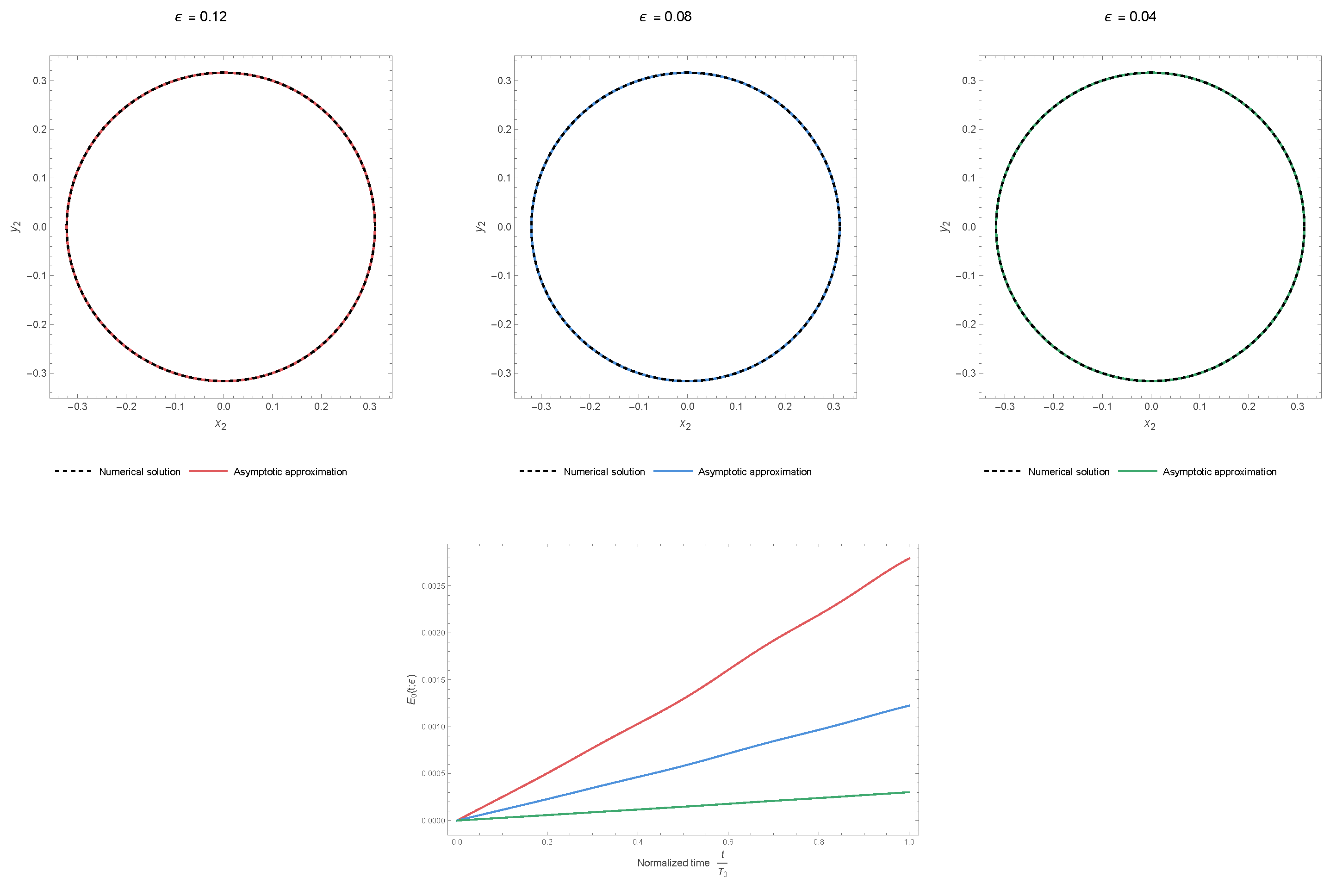
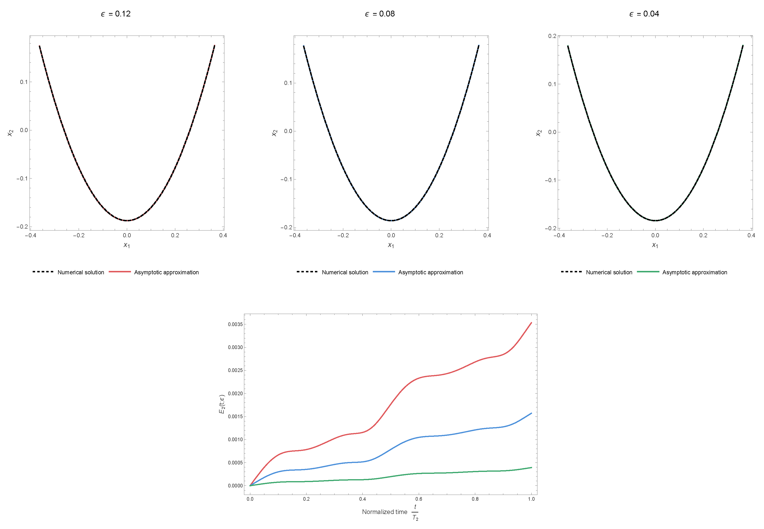
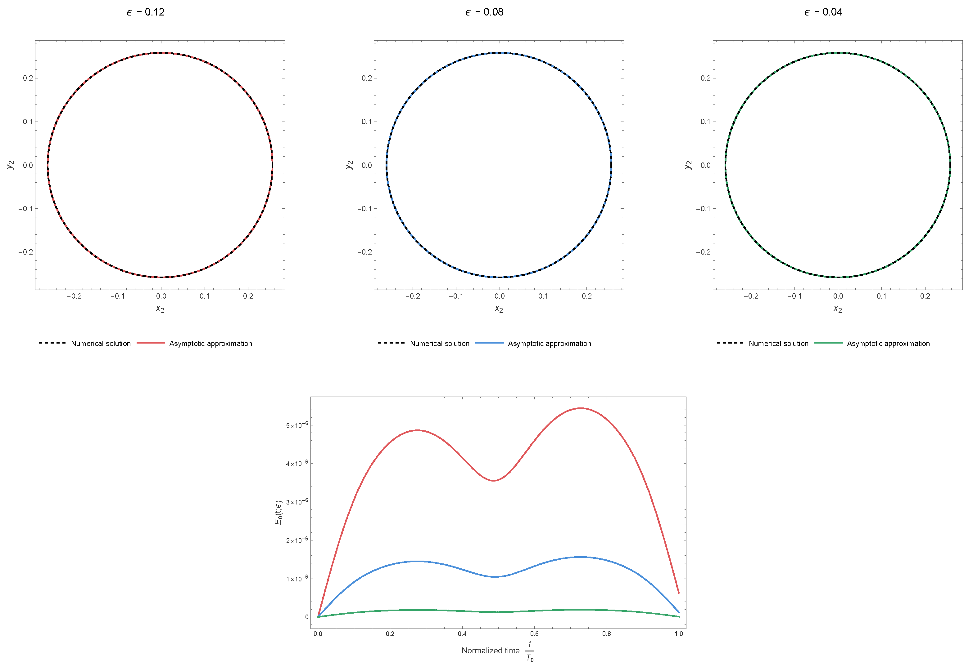
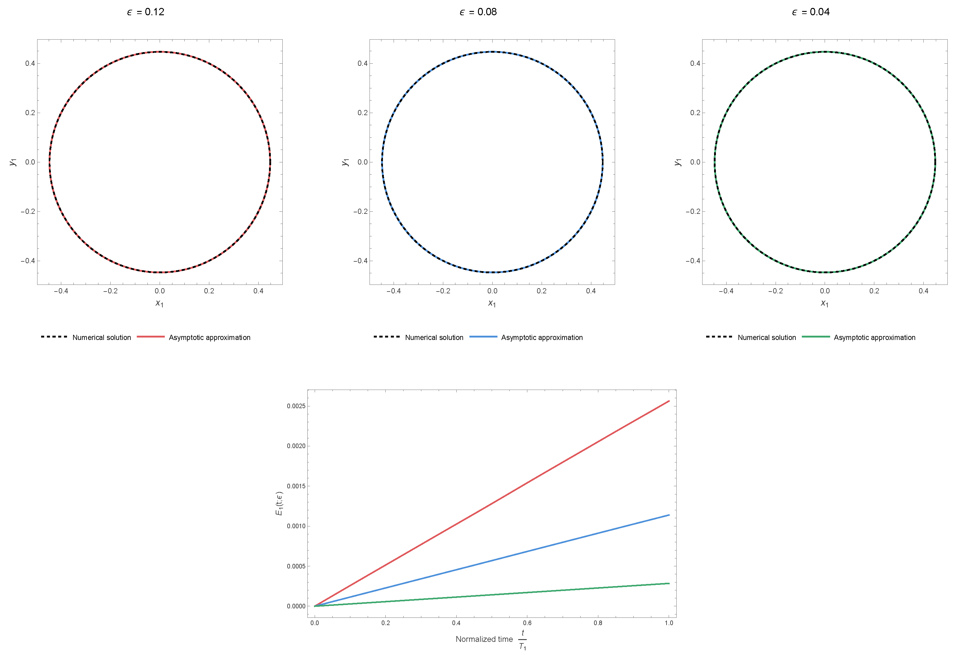
To illustrate the accuracy of the periodic approximations, we set $\alpha =\beta =1,h=0.1$, and ${\ell }_0=0,$ and compare them with numerical integrations of the full Hamiltonian system for $\epsilon =0.12,0.08,$ and $0.04$. The numerical computations and figures were obtained with Wolfram Mathematica 15.0. In physical time, the asymptotic approximation associated with ${\mathcal{O}}_j$ is defined by

$${\phi }_j^{\mathrm{app}}(t;\epsilon ):={\phi }_j\left({\ell }_0-{\Omega }_j\left(\epsilon \right)t,\epsilon \right),$$

where ${\Omega }_j\left(\epsilon \right)$ is the corresponding frequency. For each value of $\epsilon$, the numerical solution is initialized at

$${\phi }_j^{\mathrm{num}}(0;\epsilon )={\phi }_j^{\mathrm{app}}(0;\epsilon ).$$

The colored curves represent the asymptotic approximations, whereas the black dashed curves represent the numerical solutions. The approximation error is defined by

$$E_j(t;\epsilon )={∥{\phi }_j^{\mathrm{num}}(t;\epsilon )-{\phi }_j^{\mathrm{app}}(t;\epsilon )∥}_{{\mathbb{R}}^4}$$

and is displayed as a function of the normalized time $t/T_j\left(\epsilon \right)\in [0,1]$.

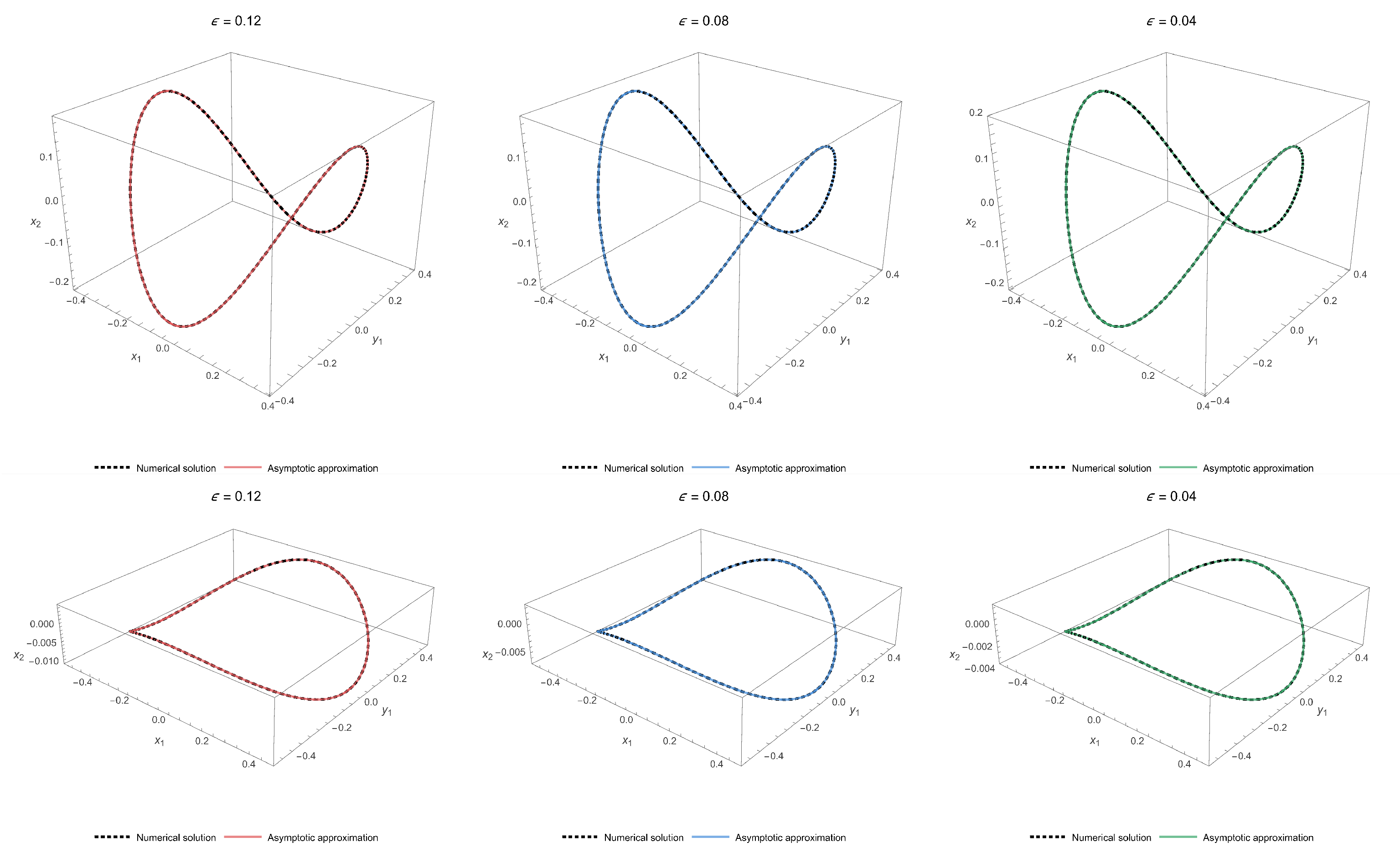
The periodic orbit associated with ${\mathcal{O}}_0$ lies in the invariant plane $x_1=y_1=0$ and is therefore represented in the $(x_2,y_2)$-plane. The regular periodic orbits associated with ${\mathcal{O}}_2$ and ${\mathcal{O}}_1$ are displayed in the $(x_1,x_2)$- and $(x_1,y_1)$-planes, respectively. Their three-dimensional projections are included in Appendix B.

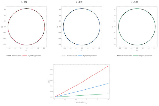
We first consider the $1:2$ resonance. Figure 2 and Figure 3 show the results associated with the singular point ${\mathcal{O}}_0$ and the regular point ${\mathcal{O}}_2$, respectively. Since the behavior associated with ${\mathcal{O}}_3$ is analogous to that associated with ${\mathcal{O}}_2$, it is not displayed.

Figure 2. Numerical and asymptotic trajectories associated with ${\mathcal{O}}_0$ for the $1:2$ resonance in the $(x_2,y_2)$-phase plane, together with the approximation error $E_0(t;\epsilon )$ over one period.

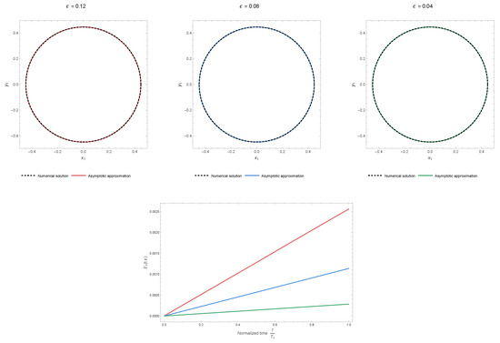
Figure 3. Numerical and asymptotic trajectories associated with ${\mathcal{O}}_2$ for the $1:2$ resonance. The upper row shows the projection onto the $(x_1,x_2)$-plane, and the lower panel shows $E_2(t;\epsilon )$ over one period.

We next consider the $1:\omega$ resonance with $\omega =3$. Figure 4 and Figure 5 show the results associated with the second and first normal modes, respectively.

Figure 4. Numerical and asymptotic trajectories associated with ${\mathcal{O}}_0$ for the $1:3$ resonance in the $(x_2,y_2)$-phase plane, together with $E_0(t;\epsilon )$ over one period.

Figure 5. Numerical and asymptotic trajectories associated with ${\mathcal{O}}_1$ for the $1:3$ resonance. The upper row shows the projection onto the $(x_1,y_1)$-plane, and the lower panel shows $E_1(t;\epsilon )$ over one period.

In all cases, the agreement between the numerical and asymptotic trajectories improves as $\epsilon$ decreases. The observed error decay is consistent with the residual orders $O\left({\epsilon }^2\right)$ for the $1:2$ resonance and $O\left({\epsilon }^3\right)$ for the $1:\omega$ resonance.

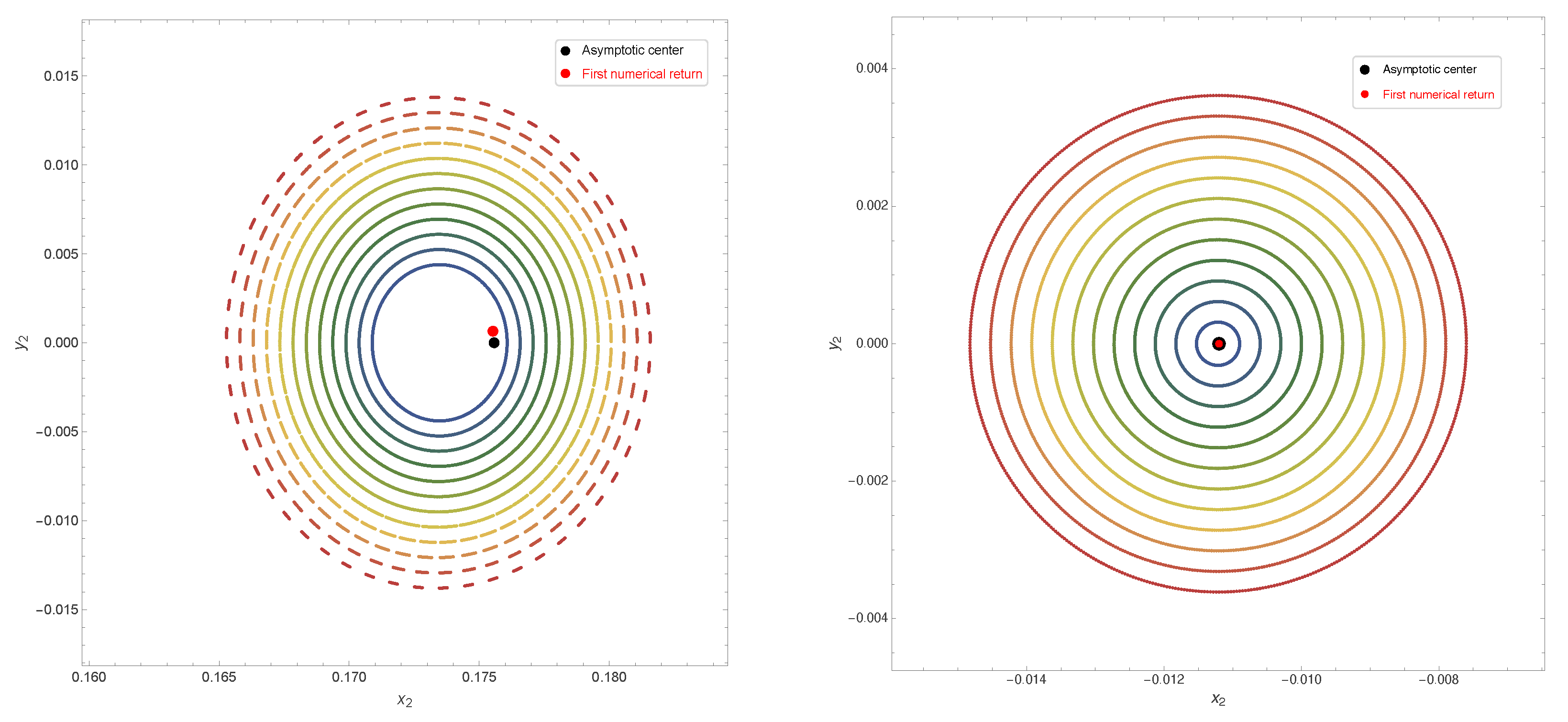
5.5. Poincaré Sections near the Stable Periodic Orbits

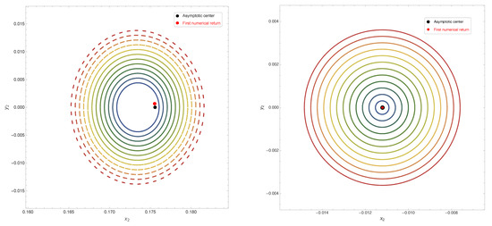
As representative examples, we illustrate the KAM structure near the stable regular periodic orbits associated with ${\mathcal{O}}_2$ for the $1:2$ resonance and with ${\mathcal{O}}_1$ for the $1:3$ resonance. We compute Poincaré sections of the full Hamiltonian system on

$$\Sigma =\left\{(x_1,x_2,y_1,y_2):{\mathcal{H}}_{\epsilon }=h,y_1=0,x_1>0\right\}$$

and represent the successive intersections in the $(x_2,y_2)$-plane. In both cases, we set

$$\alpha =\beta =1,h=0.1,\epsilon =0.12.$$

To obtain a clear and consistent representation of the invariant curves, we computed 800 successive intersections for each nearby trajectory in both cases.

The asymptotic periodic approximation is used only to determine the location of the center in the $(x_2,y_2)$-plane. Its lift to the Poincaré section, as well as the nearby initial conditions, is adjusted so that all initial points lie on the exact energy level ${\mathcal{H}}_{\epsilon }=h$. All intersections are then obtained by numerical integration of the full Hamiltonian system.

Figure 6 shows the Poincaré sections near the stable regular periodic orbits associated with ${\mathcal{O}}_2$ for the $1:2$ resonance and with ${\mathcal{O}}_1$ for the $1:3$ resonance.

Figure 6. Poincaré sections near the stable regular periodic orbits: (left) the $1:2$ resonance near ${\mathcal{O}}_2$; (right) the $1:3$ resonance near ${\mathcal{O}}_1$. The black and red points indicate the asymptotic center and the first numerical return, respectively. The colored closed curves are generated by nearby numerical trajectories of the full Hamiltonian system.

In both cases, the nested closed curves are intersections of quasi-periodic trajectories with the section and provide a numerical illustration of the KAM structure surrounding the corresponding linearly stable periodic orbit.

6. Conclusions

We studied the periodic orbits and invariant tori of the Hénon–Heiles Hamiltonian system under a $1:\omega$ resonance, with $\omega \ge 2$. The combination of Lie–Deprit normalization with regular and singular reduction provides a unified description of the regular and singular critical points of the reduced Hamiltonian and the periodic orbits associated with them.

For the $1:2$ resonance, the reduced system has three isolated critical points. The two regular critical points generate linearly stable periodic orbits with periods close to $2\pi$, whereas the periodic orbit associated with the singular peak has a period close to $\pi$ and is Lyapunov-unstable. For $\omega \ge 3$, the two normal modes generate periodic orbits with periods close to $2\pi$ and $2\pi /\omega$, respectively. Under the corresponding non-degeneracy conditions, both periodic orbits are linearly stable.

We also proved that families of two-dimensional invariant KAM tori surround the linearly stable periodic orbits. In each case, the complement of the union of these tori has measure $O\left({\epsilon }^{3/2}\right)$ for the $1:2$ resonance and $O\left({\epsilon }^2\right)$ for $\omega \ge 3$. Finally, the Lie transformations provide explicit asymptotic parametrizations of the periodic orbits in the original variables, distinguishing the first-order resonant contribution in the $1:2$ case from the second-order contribution for $\omega \ge 3$.

Direct substitution verifies the stated accuracy of the periodic approximations, while numerical integrations and Poincaré sections illustrate the nearby KAM structure. These results provide a unified local description of the periodic and quasi-periodic dynamics generated by the $1:\omega$ resonances. The degenerate parameter cases, for which the reduced Hamiltonian is constant or has a continuum of critical points at the computed order, require higher-order normalization. The next nonzero resonant term is needed to determine whether this degeneracy persists or is removed; this higher-order analysis lies beyond the scope of the present work. A further direction is to extend the analysis to general resonant frequency pairs

$$({\omega }_1,{\omega }_2)\in {(\mathbb{R}\setminus \left\{0\right\})}^2,{\displaystyle \frac{{\omega }_1}{{\omega }_2}}\in \mathbb{Q}.$$

References

- Hénon, M.; Heiles, C. The applicability of the third integral of motion: Some numerical experiments. Astron. J. 1964, 69, 73–79. [Google Scholar] [CrossRef] [Scilit]
- Braun, M. On the applicability of the third integral of motion. J. Differ. Equ. 1973, 13, 300–318. [Google Scholar] [CrossRef] [Scilit][Green Version]
- Caranicolas, N.D. Orbits in global and local galactic potentials. Astron. Astrophys. Trans. 2004, 23, 241–252. [Google Scholar] [CrossRef] [Scilit]
- Churchill, R.C.; Pecelli, G.; Rod, D.L. A survey of the Hénon–Heiles Hamiltonian with applications to related examples. In Stochastic Behavior in Classical and Quantum Hamiltonian Systems; Casati, G., Ford, J., Eds.; Lecture Notes in Physics; Springer: Berlin/Heidelberg, Germany, 1979; Volume 93, pp. 76–136. [Google Scholar] [CrossRef] [Scilit]
- Contopoulos, G.; Tzemos, A.C.; Zanias, F. Integrals and chaos in generalized Hénon–Heiles Hamiltonians. Phys. Scr. 2025, 100, 045225. [Google Scholar] [CrossRef] [Scilit]
- Bountis, T.; Segur, H.; Vivaldi, F. Integrable Hamiltonian systems and the Painlevé property. Phys. Rev. A 1982, 25, 1257–1264. [Google Scholar] [CrossRef] [Scilit]
- Grammaticos, B.; Dorizzi, B.; Padjen, R. Painlevé property and integrals of motion for the Hénon–Heiles system. Phys. Lett. A 1982, 89, 111–113. [Google Scholar] [CrossRef] [Scilit]
- Verhulst, F. Integrability and non-integrability of Hamiltonian normal forms. Acta Appl. Math. 2015, 137, 253–272. [Google Scholar] [CrossRef] [Scilit]
- Conte, R.; Musette, M.; Verhoeven, C. Completeness of the cubic and quartic Hénon–Heiles Hamiltonians. Theor. Math. Phys. 2005, 144, 888–898. [Google Scholar] [CrossRef] [Scilit]
- Wojciechowski, S. Separability of an integrable case of the Hénon–Heiles system. Phys. Lett. A 1984, 100, 277–278. [Google Scholar] [CrossRef] [Scilit]
- Ballesteros, Á.; Blasco, A. Integrable Hénon–Heiles Hamiltonians: A Poisson algebra approach. Ann. Phys. 2010, 325, 2787–2799. [Google Scholar] [CrossRef] [Scilit]
- Miller, B.R. The Lissajous transformation. III. Parametric bifurcations. Celest. Mech. Dyn. Astron. 1991, 51, 251–270. [Google Scholar] [CrossRef] [Scilit]
- Churchill, R.C.; Kummer, M.; Rod, D.L. On averaging, reduction, and symmetry in Hamiltonian systems. J. Differ. Equ. 1983, 49, 359–414. [Google Scholar] [CrossRef] [Scilit]
- Deprit, A. Canonical transformations depending on a small parameter. Celest. Mech. 1969, 1, 12–30. [Google Scholar] [CrossRef] [Scilit]
- Lanchares, V.; Pascual, A.I.; Iñarrea, M.; Salas, J.P.; Palacián, J.F.; Yanguas, P. Reeb’s theorem and periodic orbits for a rotating Hénon–Heiles potential. J. Dyn. Differ. Equ. 2021, 33, 445–461. [Google Scholar] [CrossRef] [Scilit]
- Meyer, K.R.; Palacián, J.F.; Yanguas, P. Singular reduction of resonant Hamiltonians. Nonlinearity 2018, 31, 2854–2894. [Google Scholar] [CrossRef] [Scilit]
- Gimeno, J.; Jorba, À.; Jorba-Cuscó, M.; Zou, M. Explicit numerical computation of normal forms for Poincaré maps. Commun. Nonlinear Sci. Numer. Simul. 2025, 149, 108913. [Google Scholar] [CrossRef] [Scilit]
- Han, Y.; Li, Y.; Yi, Y. Invariant tori in Hamiltonian systems with high order proper degeneracy. Ann. Henri Poincaré 2010, 10, 1419–1436. [Google Scholar] [CrossRef] [Scilit]
- Meyer, K.R.; Palacián, J.F.; Yanguas, P. Geometric averaging of Hamiltonian systems: Periodic solutions, stability, and KAM tori. SIAM J. Appl. Dyn. Syst. 2011, 10, 817–856. [Google Scholar] [CrossRef] [Scilit]
- Yanguas, P.; Palacián, J.F.; Meyer, K.R.; Dumas, H.S. Periodic solutions in Hamiltonian systems, averaging, and the lunar problem. SIAM J. Appl. Dyn. Syst. 2008, 7, 311–340. [Google Scholar] [CrossRef] [Scilit]
- Meyer, K.R.; Offin, D.C. Introduction to Hamiltonian Dynamical Systems and the N-Body Problem, 3rd ed.; Applied Mathematical Sciences; Springer: Cham, Switzerland, 2017; Volume 90. [Google Scholar] [CrossRef] [Scilit]
- Yakubovich, V.A.; Starzhinskii, V.M. Linear Differential Equations with Periodic Coefficients; Louvish, D., Translator; John Wiley & Sons: New York, NY, USA, 1975; Volume 1–2. [Google Scholar]
- Cushman, R.H.; Bates, L.M. Global Aspects of Classical Integrable Systems, 2nd ed.; Birkhäuser: Basel, Switzerland, 2015. [Google Scholar] [CrossRef] [Scilit]
- Marsden, J.E.; Weinstein, A. Reduction of symplectic manifolds with symmetry. Rep. Math. Phys. 1974, 5, 121–130. [Google Scholar] [CrossRef] [Scilit]
- Meyer, K.R. Symmetries and integrals in mechanics. In Dynamical Systems; Peixoto, M.M., Ed.; Academic Press: New York, NY, USA, 1973; pp. 259–272. [Google Scholar] [CrossRef] [Scilit]
- Reeb, G. Sur certaines propriétés topologiques des trajectoires des systèmes dynamiques. In Mémoires de l’Académie Royale de Belgique, Classe des Sciences, Collection in-8°, 2e Série; Ort, Verlag: Bruxelles, Belgium, 1952; Volume 27, pp. 1–64. [Google Scholar]
Disclaimer/Publisher’s Note: The statements, opinions and data contained in all publications are solely those of the individual author(s) and contributor(s) and not of MDPI and/or the editor(s). MDPI and/or the editor(s) disclaim responsibility for any injury to people or property resulting from any ideas, methods, instructions or products referred to in the content. |
© 2026 by the authors. Licensee MDPI, Basel, Switzerland. This article is an open access article distributed under the terms and conditions of the Creative Commons Attribution (CC BY) license.