


Abstract
Complex Network Analysis (CNA) models river systems as networks of nodes (junctions) and edges (channels) to quantify structure and potential transport pathways. Unlike conventional river-network characterization, which often relies on multiple metric-specific analyses of stream hierarchy, branching, drainage density, and topographic characteristics, a graph-based approach provides a unified mathematical framework to assess the entire structural topology and connectivity of the basin simultaneously. In this study, the river networks of Leyte Island were analyzed using 5 m-resolution Interferometric Synthetic Aperture Radar (IfSAR)-derived Digital Terrain Model (DTM) data. River networks were represented as upstream-to-downstream direction graphs, with flow direction assigned based on elevation, and key network parameters, including the number of nodes, average degree centrality, closeness centrality, clustering coefficient, and betweenness centrality, were computed. Simple river networks consisting of two nodes were dominant across Leyte Island, while relatively few large and structurally complex networks were identified. The network metrics generally indicated tree-like or dendritic topologies. Comparison with randomly generated tree networks revealed both similarities and differences in several network metrics across different network sizes. Although both network types exhibit tree-like structures and consequently have zero average clustering coefficients, the differences in other metrics suggest that river networks may exhibit structural characteristics that are not fully represented by randomly generated tree networks. Slope analysis revealed a significant but weak negative correlation between river-network slope and the number of nodes. A key strength of CNA is its data-driven integration of topographic information into the network design, such as slope and elevation, enabling consistent and reproducible characterization of river networks. Future work could further enhance the accuracy of river-network representation through additional spatial validation using higher-resolution geospatial data.
1. Introduction
Rivers constitute independent ecological systems characterized by their linear organization within interconnected and dynamic network structures [1]. These networks serve as critical channels for the distribution of water between ecological environments and human societies, playing an essential role in sustaining both systems amid ongoing global change [1]. River network structure refers to the spatial and geometric arrangement of its components, encompassing the lengths, positions, and connectivity of individual streams, together with the overall organization and topology of the entire system [2]. Characterizing the structure of river networks is essential because it provides insight into hydrologic connectivity, which governs the movement and transport of water, sediments, nutrients, and pollutants within a catchment system [3,4]. River network parameters describe the geometric and structural properties of a drainage system and provide the basis for quantitatively classifying different river network types, offering valuable insights for the development of hydrological models that can support more effective flood risk assessment and disaster preparedness [5,6]. Furthermore, several studies have demonstrated that the structural configuration of river networks can influence and be associated with water and ecological quality and biodiversity [7,8,9,10]. Theoretical and empirical studies from Carrara et al. [11] and Terui et al. [12] suggest that the structure of network topology plays a crucial role in sustaining metapopulation stability and shaping patterns of biodiversity.
A variety of parameters have been proposed to characterize the structural properties of river networks, including river density [5], water surface ratio [8], river flow direction [5], river sinuosity [5], and fractal dimension [2]. River networks form complex and spatially heterogeneous systems whose structural characteristics are challenging to describe using simple morphological indicators alone [2]. Although these measures offer valuable insights into river network structure, they rely on datasets encompassing both natural and artificial features, which may not always be accessible or complete in all regions.
Complex network analysis (CNA) applies concepts from graph theory that can quantify topological and topographic indices that describe river connectivity and structure [4]. A number of studies have represented river networks as directed graphs characterized by complex topologies, in which vertices or nodes are linked by directed edges corresponding to the flow direction of water [3,4,13,14,15,16]. Some studies model rivers as complex networks using graph theory, allowing the characterization of river structure and connectivity through simulation algorithms and network metrics [13,15,16,17]. Others focus on employing CNA metrics as indicators of hydrological connectivity [3,8], while some apply these approaches directly to real river systems to assess their structural and functional properties [4].
CNA facilitates both the visualization and quantitative evaluation of connectivity within river basins and delta channels [3]. While many available metrics may exhibit uncertainty in reflecting actual functional connectivity, betweenness centrality, a metric derived from CNA, has emerged as both a reliable and consistent indicator of river network connectivity, which is important in assessing the functional role of key river junctions and guiding watershed management and conservation strategies [18]. CNA can also be used to compute environmental impact indices by modeling pollutant transport and dispersion throughout river systems, enabling assessment of how network structure influences environmental connectivity and contamination pathways [4]. CNA provides a systematic and sophisticated framework for representing interactions within river systems and for examining their underlying structure and dynamics. A major advantage of CNA over traditional in situ observations is that it enables the analysis of river networks remotely using readily available satellite-derived data, reducing the need for extensive fieldwork while facilitating comprehensive, large-scale assessments. Geospatial analysis techniques and satellite observations have been widely employed in river system analysis, as demonstrated in several studies [19,20,21,22]. Their applications vary from the characterization of river networks through the development of functional process zone nomenclature [19] to the estimation of total river surface area [20,21] and the calculation of river width [22].
Most studies applying CNA have primarily focused on the structure of individual river basins, such as the Guadalquivir River Basin in southern Spain [4], or on theoretical and simulated river network models [13,16]. Comparatively less attention has been given to the systematic application of graph-based metrics across multiple drainage systems within a common geographic setting. An island provides a well-defined geographic domain for such an analysis, allowing multiple river networks to be characterized using a consistent framework and compared across contrasting topographic settings. This approach enables the identification of differences and similarities in network organization among drainage systems that may not be apparent from studies of individual catchments. However, graph-based studies that systematically characterize and compare multiple river networks across an entire island remain limited.
The overall aim of this study is therefore to characterize and compare the structural organization of river networks across Leyte Island, Philippines, using a consistent CNA framework. Specifically, the study aims to (1) characterize the distribution of river-network size and topology across the island using the number of nodes, average degree, closeness centrality, clustering coefficient, and betweenness centrality; (2) determine the extent to which variation in these graph metrics is associated with overall network size; (3) test whether network size and complexity differ between steep and low-gradient catchments; and (4) assess the sensitivity of river-network metrics to variations in the processing parameters used during the extraction and graph representation of river networks. By addressing these objectives, the study provides a consistent graph-based inventory of Leyte’s drainage systems and a reproducible workflow for extracting, characterizing, and comparing multiple river networks from high-resolution topographic data.
By examining river networks at this broader spatial scale, the research offers a more comprehensive understanding of hydrological organization and generates valuable insights that may support island-wide water resource management, ecological assessment, and environmental planning. Furthermore, integrating complex network metrics with geomorphological and hydrological processes will provide new perspectives on connectivity, system resilience, and flood dynamics in small, steep, and highly dynamic tropical catchments. Focusing on a typhoon-prone tropical island also highlights the potential of linking the structural properties derived from this study to future flood hazard and hydrological modeling applications.
2. Methodology
2.1. Study Area
Leyte Island covers approximately 7368 km2 and is the eighth-largest island in the Philippines (Figure 1) [23]. Leyte Island, located in Region VIII (Eastern Visayas) in the central Philippines, is composed of the provinces of Leyte and Southern Leyte. Leyte province is administratively divided into five congressional districts, comprising two cities and 40 municipalities, and encompasses a total of 1478 barangays (i.e., villages) and a population of about 1.8 million based on the 2024 census [24,25]. The province of Southern Leyte has 1 city, 18 municipalities, and 500 barangays and has a population of approximately 430 thousand [25,26].
Figure 1.
Map of Leyte Island showing the municipalities and the island’s location within the Philippines. Grid coordinates are expressed in meters using the PRS92/Philippines Zone 5 coordinate reference system (EPSG:3125).
Based on the thirty-two (32) water bodies in Leyte Island listed by the Environmental Monitoring Bureau of the Department of Environment and Natural Resources (EMB-DENR) [27], most of them (78%) are classified as Class C (waters support a range of uses, including fisheries, secondary recreational activities like boating and fishing, and agricultural purposes such as irrigation and livestock watering). Only a small portion falls under Class A (waters need full conventional treatment—coagulation, sedimentation, filtration, and disinfection) or Class B (waters are intended for primary contact recreation, such as swimming and bathing) [27].
In terms of ecological water quality, Forio et al. [23] indicated that many of the studied river sites exhibited good to very good ecological quality class based on the Biological Monitoring Working Party-Vietnam (BMWP-Viet) index. The southern part of the island or the mountainous regions constitute the most diverse sites in terms of macroinvertebrate composition, while the west coast has low diversity. This makes Leyte Island an interesting location for complex network analysis of river systems.
2.2. Open Street Map and DEM-Derived River Networks Comparison
River networks derived from OpenStreetMap (OSM) and DEM were compared to evaluate their structural and spatial agreement.
2.2.1. River Network Derived from Open Street Map
River network data for Leyte, Eastern Visayas, Philippines, were obtained from OpenStreetMap (OSM) using the BBBike OpenStreetMap Extract Service version 3.18. The extraction covered the geographic extent of 124.051–125.396° E longitude and 9.820–11.736° N latitude, encompassing the study area of Leyte Island. The data were downloaded in GeoPackage (.gpkg) format and used as the reference river network for comparison with the 5 m Interferometric Synthetic Aperture Radar Digital Terrain Model (5 m IfSAR DTM)-derived river network.
The extracted dataset covered an area of approximately 31,402 km2 and had a granularity of 100, corresponding to approximately 1.1 cm in the extracted map representation. The OSM database used for the extraction was last updated on 11 August 2026 at 23:00 UTC. The dataset was obtained under the OpenStreetMap [28] License.
The OSM river network was subsequently processed in QGIS [29] version 3.40.10 Bratislava to identify and extract river channels within the study area. The resulting network was used as the reference dataset for evaluating the channel omission, channel addition, and positional agreement of the 5 m IfSAR DTM river network.
2.2.2. DEM-Derived River Network
The river network used in this study was obtained from the Geospatial Research, Innovation, and Development (GRID) Center of Visayas State University (VSU), Baybay, Leyte. The river network shapefile was generated through the processing of elevation data using Geographic Information System (GIS) techniques and was provided by the GRID Center for use in the present study. The elevation data underlying the river network are products of the Philippine Light Detection and Ranging (Phil-LiDAR) Program [30], a nationwide geospatial mapping initiative implemented through the Department of Science and Technology (DOST), the University of the Philippines, and participating State Universities and Colleges (SUCs) and Higher Education Institutions (HEIs). The Phil-LiDAR Program developed from the Disaster Risk and Exposure Assessment for Mitigation (DREAM) Program, which was established to generate detailed and high-resolution three-dimensional elevation and flood-hazard information for Philippine river basins. The river network dataset was provided as an ESRI Shapefile consisting of 1229 MultiLineString features and was referenced to the WGS 84 geographic coordinate system (EPSG:4326). The dataset covers approximately 124.284–125.294° E and 9.937–11.548° N.
The river network represents a drainage network extracted from elevation data rather than a directly mapped river inventory. Although LiDAR-derived elevation data provide substantially finer spatial information than conventional remotely sensed elevation products, complete high-resolution LiDAR coverage is not available across all areas of Leyte. A 5 m resolution IfSAR-derived DTM of Leyte Island was used as the elevation source for the analysis. The DTM was provided as a single-band GeoTIFF raster with 32-bit floating-point elevation values and a spatial resolution of 5 m × 5 m. The raster contained elevation values ranging from 0 to 1098.46 m, with a mean elevation of 180.34 m and a standard deviation of 209.91 m. The DTM was used to extract elevation values along the river network and to calculate elevation differences and river-channel slopes.
2.2.3. Comparison Methodology
Three river networks representing different levels of network complexity were randomly selected for comparative analysis based on the number of nodes: (1) a simple network with two nodes, (2) an intermediate network with 10–15 nodes, and (3) a complex network with more than 40 nodes. The selection of networks with varying numbers of nodes was intended to assess whether differences between DEM-derived and OSM-derived river networks vary with network complexity.
For each selected river network, the total channel length was calculated separately for the DEM-derived and OSM-derived datasets. The ratio of the total DEM-derived channel length to the corresponding OSM-derived channel length was then calculated using the following:
where RL is the channel-length ratio, LDEM is the total channel length of the DEM-derived network, and LOSM is the total channel length of the OSM-derived network.
The river networks with more than 40 nodes, representing the more complex networks, were subjected to a more detailed spatial comparison. This analysis evaluated three primary characteristics: (1) channel omission, (2) channel addition, and (3) positional agreement. Channel omission refers to channels present in the OSM-derived network but absent from the DEM-derived network, while channel addition refers to channels identified in the DEM-derived network that were not represented in the OSM-derived network. Positional agreement was assessed by examining the spatial correspondence between the two networks, including their general alignment, connectivity, and representation of channel patterns such as meandering.
2.3. River Network Processing
The overall methodological workflow is summarized in Figure 2.
Figure 2.
General flowchart of the methodology.
Considering an actual river system shown in Figure 3A, river networks were derived using a 5 m IfSAR DTM. This river network (Figure 3B) can then be transformed into a directed graph (Figure 3C), where arrows indicate the direction of water flow. In this representation, node 1, 2 and 3 correspond to the river sources, node 4 and 5 represent branching junctions where the river diverges into multiple channels, and node 6 indicate the outlet where the river discharges into the ocean. It should also be noted that a node may represent a converging junction, where two or more tributaries meet and merge within the river network.
Figure 3.
Illustration of the river network and directed graph generation. Based on the generated directed graphs and nodes, network metrics were derived. (A) Actual river system; (B) derived river network; and (C) corresponding directed graph, with arrows indicating the direction of water flow.
The overall workflow for processing and extracting the river network is illustrated in Figure 4 below.
Figure 4.
River network processing workflow.
2.3.1. River Network Preprocessing
To determine the most appropriate image thresholding technique for extracting river networks from rasterized river data, several thresholding methods available in the scikit-image (skimage) v0.19.2 library [31], implemented using Python v3.9.12 [32], were evaluated. The analysis included nine thresholding techniques: Isodata [33], Li [34], Local [34,35], Mean [36], Minimum [37], Niblack [38], Sauvola [39], Triangle [40], Yen [41], and Otsu [42]. Additional information is found in Supplementary Note S1.
Additionally, details on filtering/removing spurious nodes can be found in Supplementary Note S2, which describes the methodology when the initial node-detection procedure generally produced a higher number of nodes than the expected or reference network; an additional node-filtering procedure based on a spatial distance threshold was implemented.
2.3.2. River Network Data Processing
The 5 m IfSAR DTM river network shapefile processed in QGIS version 3.40.10-Bratislava [29] is shown in Figure 5A. River length data were obtained using the edge length measurement module in QGIS, which calculates the total length of each river segment based on the spatial geometry of the vector river network. This approach ensures accurate representation of river extents by accounting for meanders and curvature, allowing for precise quantification of river network structure and facilitating subsequent analyses of connectivity, network metrics, and spatial patterns across the study area.
Figure 5.
Workflow for converting river networks into directed graph representations (A) Selected river network used as the input dataset; (B) conversion of the river network into a binary raster image, with river channels represented as continuous linear features; (C) thresholding and skeletonization to produce single-pixel-wide representations of the river channels; (D) automated node detection and generation from the processed network, followed by distance-based filtering to remove spurious nodes; (E) assignment of flow direction to network edges based on upstream-to-downstream elevation, resulting in a directed network; and (F) calculation of key network metrics, including in-degree and out-degree, degree centrality, closeness centrality, clustering coefficient, and betweenness centrality.
Each river network was then imported into Python v3.9.12 [32] and converted into a directed graph representation using the NetworkX v2.7.1 library [43].
The direction of the river network was assigned based on the elevation information derived from the IfSAR Digital Terrain Model (DTM). Elevation values were extracted for the nodes and/or river-segment endpoints, and the relative elevation of connected locations was used to establish the direction of flow. River segments were oriented from locations with higher elevation (upstream) toward locations with lower elevation (downstream), consistent with the natural tendency of surface water to flow downslope. This procedure converted the extracted river network into a directed graph, where each directed edge represents a river segment and its orientation corresponds to the inferred flow direction.
The preprocessing workflow involved delineating selected river networks and converting them into binary raster images (Figure 5B), where river channels were represented as continuous linear features. Image processing techniques, including thresholding and skeletonization (implemented using scikit-image), were applied to reduce the river network to single-pixel-wide paths representing flow channels (Figure 5C). Nodes were then identified and generated from the processed network (Figure 5D). Additional filtering of nodes was performed using a distance threshold to remove spurious nodes introduced during the automated detection process.
Flow direction was subsequently assigned to each edge to reflect the natural direction of river flow (Figure 5E), resulting in a directed network representation. Finally, key network metrics, including in-degree and out-degree, degree centrality, closeness centrality, clustering coefficient, and betweenness centrality (Figure 5F), were computed to characterize the network properties of each river network.
River networks for which flow direction could not be reliably determined, particularly those lacking clear downstream continuity toward a receiving water body such as a lake or the ocean, were excluded from the analysis. River networks that exhibited discontinuities or ambiguities resulting from the thresholding process, such that network nodes could not be clearly identified and represented, were likewise excluded. These exclusion criteria were applied to ensure that only river networks with sufficiently clear spatial continuity, identifiable nodes, and reliable flow direction were included in the subsequent network analysis. This study adopts a rivers-to-sea perspective [44] or ridge-to-reef model [45], which emphasizes the connectivity between land-based activities, freshwater drainage systems, coastal environments, and the ocean. Rivers play a critical role in ocean forecasting by influencing coastal and basin-scale circulation through their hydrological and biogeochemical inputs, which affect water-mass distribution, mixing, and upwelling processes [46]. River networks provide a principal pathway through which water and land-derived materials can be transported from terrestrial catchments toward coastal and marine environments. This perspective is particularly relevant to island systems such as Leyte, where surface drainage generally converges toward coastal outlets. Accordingly, the present study considers only river networks with a continuous downstream connection to the ocean. This criterion does not imply that internally draining or disconnected river systems are ecologically unimportant; rather, it defines the scope of the analysis around land-to-ocean connectivity and enables the structural characteristics of river networks to be interpreted in relation to their potential role in connecting land-based populations and activities with downstream coastal and marine environments.
2.4. River Network Metrics
The equations, definitions, and implications of the network metrics are summarized in the Table 1 below. More detailed illustrations and explanations are provided in Supplementary Note S3.
Table 1.
Summary of network metrics, equations, and their definitions and implications.
Python NetworkX Implementation
The river networks were represented as directed graphs using NetworkX (nx.DiGraph), with edges oriented from upstream to downstream according to the direction of river flow. Network metrics were then calculated to characterize the structural properties of each network (Table 2). Degree centrality was computed to quantify overall node connectivity, while in-degree and out-degree centrality were calculated separately to describe the number of upstream connections entering and downstream connections leaving each node, respectively. Closeness centrality was used to measure the accessibility of nodes within the directed network, clustering coefficient to quantify the local interconnectedness of neighboring nodes, and betweenness centrality to identify nodes that frequently occur along shortest paths between other nodes. The mean values of these node-level metrics were subsequently calculated to obtain an overall structural characterization of each river network.
Table 2.
Summary of network metrics and corresponding NetworkX code.
The river network was represented as a directed graph to account for the direction of flow within the network. The corresponding NetworkX code and implementation details are provided in the associated GitHub repository [50], while additional information on the use and implementation of NetworkX can be found in [47].
2.5. River Network Slope Analysis
The DEM-derived river network was first reprojected to EPSG:32651 (WGS 84/UTM Zone 51N) to ensure that distances were expressed in meters. The river segments were then draped over the 5 m IFSAR DTM in QGIS to assign elevation values to the vertices of each river segment. The first (z_first) and last (z_last) elevation values extracted from the draped network were used to determine the elevation difference (ΔZ) between the endpoints, while the segment length (L) was obtained from the reprojected river geometry. The longitudinal slope S(%) of each river segment was then calculated as follows:
where Zfirst and Zlast are the extracted elevations at the first and last vertices, respectively, and L is the river-segment length in meters. The absolute value was used to express the magnitude of the elevation gradient, regardless of the digitized direction of the river segment.
For multiple interconnected river networks, the average slope was calculated across the individual river segments to obtain an overall slope value for the network.
3. Results
3.1. Comparison of DEM-Derived and OSM-Derived River Networks
3.1.1. Total Length Ratio
As shown in Table 3, rivers with simpler network structures, characterized by a smaller number of nodes and fewer interconnected channels, tend to exhibit a higher total length ratio closer to 1. This indicates that the total river length derived from the 5m-IFSAR DTM river network is relatively comparable to that of the reference OSM network, indicating greater agreement between the two datasets than observed for more complex river networks. More complex networks, such as rivers with nodes greater than 40 and highly interconnected river networks, tend to have a lower total length ratio, reflecting a larger discrepancy in the total channel length between the DEM-derived and OSM networks. This difference may arise from the DEM’s tendency to omit smaller tributaries, simplify meandering patterns, or introduce additional channels, resulting in greater structural differences between the two representations.
Table 3.
Total length ratio of DEM-derived and OSM-derived river networks.
3.1.2. Assessment of River Channel Positional Agreement, Omission, and Addition
A general trend in the positional agreement of the data (DEM and OSM) was observed for all samples; it was shown that DEM data is parallel to OSM data, but it was not able to capture the meanderings. The analysis of complex river networks in terms of channel omission, addition, and positional agreement is discussed further below, considering three complex river cases with more than 40 nodes: the Binahaan River, Daguitan River Complex, and Pagsangahan River Complex. Detailed results and illustrations of the comparison between the OSM- and DEM-derived river networks are provided in Supplementary Note S4. A summary of the key findings is presented below:
Case 1: Binahaan River
The comparison identified 19 omitted channels and 41 additional channels in the DEM-derived network relative to OSM. The results indicate that the DEM-derived network generally captures the major spatial configuration of the Binahaan River complex but differs from OSM in channel density, connectivity, and representation of fine-scale meandering. The DEM-derived network tends to produce a more complex channel structure while occasionally failing to preserve specific connections or smaller meandering channels represented in OSM.
Case 2: Daguitan River Complex
The comparison shows that the DEM-derived network generally follows the major spatial alignment of the OSM river network but has limitations in representing the finer-scale complexity of river meandering. The degree of channel omission and addition varies among the rivers, with the largest discrepancy observed in the Marabang River.
Case 3: Pagsangahan River Complex
The Pagsangahan River Complex had 136 omitted channels and 29 additional channels in the DEM-derived network relative to OSM. The comparison indicates that the DEM-derived network generally preserves the broad spatial alignment of the major rivers but substantially simplifies the finer-scale channel structure, particularly the smaller tributaries and meandering patterns. The most substantial discrepancies were observed in Bagalongon, Matagob, and Casa, where numerous OSM channels were omitted or, in the cases of Matagob and Casa, the entire river networks were absent from the DEM-derived data.
The DEM-derived river network was used for data processing and calculation of the network metrics presented in the succeeding sections.
3.2. River Network Preprocessing Results
A summary of the relative differences in the number of detected nodes produced by the different thresholding methods is presented in Table 4 below and illustrated in Figure 6. The results showed that the initial node-detection procedure generally produced a higher number of nodes than the expected or suitable number of nodes, as discussed in Supplemental Note S1. This overestimation may be attributed to the presence of false or spurious nodes generated during image thresholding and skeletonization. Such false nodes may arise from small artifacts, irregularities in the extracted channel boundaries, fragmented channel segments, or minor branches that do not represent meaningful river-network junctions. Among the evaluated methods, otsu, isodata, li, minimum, and sauvola produced promising results for river network segmentation. Otsu’s thresholding method was selected because it is a simple, efficient, parameter-free, and reproducible method for consistent processing of the river-network datasets [51]. An additional filtering method was implemented as discussed in the Supplementary Note S2 to remove spurious nodes.
Table 4.
Thresholding method and node count.
Figure 6.
Thresholding methods for sample node count and placement.
The effect of varying the distance threshold is summarized in the Supplementary Table S1. A low distance threshold is insufficient to remove spurious nodes, whereas an intermediate range (2.5–6) effectively filters these nodes while preserving the essential network structure. In contrast, excessively high distance thresholds may eliminate important nodes, as illustrated in Figure 7.
Figure 7.
Illustration of varying the distance threshold on the number of retained nodes.
3.3. Network Metric Results for the Analyzed River Network
The analysis identified 256 distinct river systems across Leyte Island, exhibiting a broad range of network configurations, from relatively simple drainage patterns to more complex and highly interconnected structures. The summary statistics of the resulting network metrics are presented in Table 5 below.
Table 5.
Statistical summary of the network characteristics of river systems in Leyte Island.
3.3.1. Number of Nodes, Average in and out Degree
A Pearson correlation analysis revealed an exceptionally strong, statistically significant positive linear relationship between the number of nodes and total river length (r = 0.92, p < 0.001), illustrated in Figure 8. This indicates that river networks with a higher density or count of nodes consistently correspond to greater total stream lengths across the analyzed catchments.
Figure 8.
Relationship between network complexity (number of nodes) and scale (total river length). A strong, positive linear correlation is observed (r = 0.92, p < 0.001), with the linear regression trendline (red) indicating that 84.5% of the variance in total channel length is explained by node count (R2 = 0.845).
Single-river networks, defined as river networks consisting of two nodes, comprise the dominant network configuration in the dataset, as shown in Figure 9. Further analysis of these two-node river networks indicates that their edge lengths exhibit a characteristic distribution, as illustrated in Supplementary Figure S1. The distribution of total edge lengths shows that most two-node river networks fall within the 1001–3000 m range. The frequency generally decreases as edge length increases beyond 3000 m, while very short networks (<1000 m) are relatively less common. Only a small number of relatively long (>5000 m) two-node river networks are observed.
Figure 9.
Distribution of the river network in terms of the number of nodes.
The majority of the river systems in Leyte Island are composed of small and less complex drainage networks. In contrast, only a few river networks exhibit significantly larger sizes, reflected by higher node counts and longer total edge lengths. These larger systems show a roughly linear increase in total edge length as the number of nodes increases, suggesting that as the network grows, additional river segments are added in a proportional manner. This pattern highlights the dominance of small river systems in the region while indicating the presence of a limited number of extensive river networks that contribute significantly to the island’s overall drainage structure.
The average out-degree (Figure 10) and average out-degree centrality (Figure 11) of the river systems in Leyte Island, Philippines, are presented below. The distributions of in-degree and out-degree, as well as the corresponding average in-degree and out-degree centrality, exhibit similar patterns, as expected from graph theory. When river networks consisting of a single edge are considered, the average in-degree and out-degree centrality commonly take a value of approximately 0.5. In contrast, excluding these single-edge networks results in a more diverse distribution of centrality values, reflecting greater variation in the network complexity of the river systems.
Figure 10.
Average out-degree of river networks.
Figure 11.
Average out-degree centrality of river networks.
3.3.2. Average Clustering Coefficient
Almost no triangular connections were observed in the river networks, as indicated by the average clustering coefficient being zero for 98% of the networks (Figure 12). Even after excluding single-edge networks, 94% of the networks retained an average clustering coefficient of zero, indicating that triangular or locally interconnected structures are largely absent from the analyzed river networks. This suggests that the rivers are predominantly arranged in tree-like or branching structures with minimal loops, meaning that most river segments connect in a hierarchical, linear manner rather than forming closed cycles. This structural characteristic is typical of dendritic drainage patterns.
Figure 12.
Average clustering pie chart of river networks.
3.3.3. Average Closeness Centrality
The observed peak near 0.5 in Figure 13 may reflect the predominance of small and structurally simple river networks, including single-edge and short-chain configurations, where the limited network extent results in relatively high normalized closeness values. For average closeness centrality excluding the single-edged river networks, average closeness centrality varied substantially among the river networks, with most networks exhibiting relatively low-to-moderate values and one network showing a pronounced maximum. The higher closeness values indicate that nodes within these networks are separated by relatively short, directed paths. This pattern may be associated with differences in network size and topology, as smaller and structurally compact networks generally produce shorter path distances and consequently higher normalized closeness values. Thus, the observed maximum should not necessarily be interpreted as greater network complexity but rather as greater structural proximity among the nodes within the network.
Figure 13.
Average closeness centrality of river networks.
3.3.4. Average Betweenness Centrality
The betweenness centrality of all nodes within each individual river network was computed to quantify the relative importance of nodes in facilitating connectivity and flow across the network. Sample illustrations of these computations are presented below in Figure 14 and Figure 15, highlighting key junctions that serve as critical pathways for water, sediment, and nutrient transport, as well as nodes with lower centrality that occupy peripheral or terminal positions within the river system. These visualizations provide an intuitive representation of how flow and connectivity are distributed throughout the network and allow for the identification of structurally significant nodes that may influence hydrological and ecological processes.
Figure 14.
Sample betweenness centrality values of different Leyte Island river networks.
Figure 15.
Spatial distribution of river-network nodes with high betweenness centrality across Leyte Island. Orange and red dots represent networks with 5–40 nodes, with betweenness centrality values of 0.20–0.29 and ≥0.30, respectively. Purple dots represent networks with more than 40 nodes, with betweenness centrality values of 0.025–0.09.
Most average betweenness centrality values are close to zero (Figure 16), indicating that the majority of nodes in the river network do not serve as critical intermediaries for the flow between other nodes. In other words, most river junctions are not positioned along the shortest paths connecting different parts of the network and therefore play a limited role in controlling connectivity or flow transfer across the system. This pattern suggests that only a small number of nodes act as key bridging points or major confluences where multiple tributaries merge. Such a distribution of betweenness centrality is typical of river systems that exhibit a predominantly branching or dendritic structure, where flow paths are largely direct and hierarchical rather than highly interconnected. As a result, only a few strategically located junctions significantly influence the overall connectivity and transport processes within the river network. Producing different betweenness centrality maps enables the identification of critical nodes within the river network, as illustrated in Figure 15. These high-centrality nodes represent key connectivity points that play a significant role in maintaining flow continuity and structural integrity of the river system. Their identification is important, as they often correspond to strategic locations for understanding hydrological connectivity, potential flow bottlenecks, and areas that may be highly sensitive to environmental changes or disturbances.
Figure 16.
Average betweenness centrality of river networks.
3.3.5. Comparison of River Network Metrics with Random Tree Networks
The network metrics of the generated river networks and randomly generated tree networks are presented in Table 6, with the corresponding sample graphical comparisons illustrated in the Supplementary Figure S5. For each specified number of nodes, 10 random-tree trials were generated, and the average network metrics across the trials are reported in the table.
Table 6.
Network metrics of the generated random tree networks.
The network metrics of the river networks were calculated as the average values across the nodes of individual rivers, grouped according to the corresponding number of nodes. The resulting averaged network metrics are presented in Table 7 below.
Table 7.
Average network metrics of river networks across different numbers of nodes.
The comparison with randomly generated tree networks provides a baseline for assessing whether the structural characteristics of the extracted river networks differ from those expected under random branching. Comparison with randomly generated tree networks revealed both similarities and differences in several network metrics across different network sizes. The average in-degree and out-degree centrality showed similar values between the river and random tree networks for networks with 10 and 15 nodes (illustrated in Supplementary Figures S3 and S4), but differed for networks with 5 nodes (illustrated in Supplementary Figure S2). In contrast, the average betweenness and closeness centrality differed between the two network types for networks with 10 and 15 nodes (illustrated in Supplementary Figures S3 and S4). For the 5-node networks (illustrated in Supplementary Figure S2), however, the relatively large standard deviations indicate substantial variability, such that the observed differences were not statistically significant. Although both network types exhibit tree-like structures and consequently have zero average clustering coefficients, the differences in other metrics suggest that river networks may exhibit structural characteristics that are not fully represented by randomly generated tree networks. Actual river networks are constrained by topography, elevation gradients, drainage patterns, and hydrological processes. Consequently, differences in network metrics between the observed and random networks may reflect the influence of these physical and hydrological constraints on the organization and development of river networks. These constraints can be captured within the network representation used in CNA, where the design of the graph incorporates relevant spatial and hydrological characteristics of the river system. For example, representing the network as a directed graph preserves the inferred upstream-to-downstream flow direction associated with differences in elevation among connected nodes, while the resulting network topology captures the branching and connectivity patterns imposed by the underlying terrain. Thus, CNA provides a means of quantifying how these physical and hydrological constraints are reflected in the structural organization of river networks.
3.4. Relationship Between River Slope and Network Structure
Figure 17 presents a spatial representation of Leyte Island, illustrating the distribution of river networks with varying levels of network complexity and their corresponding slope values. The areas characterized by more complex river networks generally coincide with catchments larger than 250 km2, consistent with the catchment characteristics reported for Leyte Island by Boothroyd et al. [52]. The maps show that low-slope rivers (0–0.2160%), represented predominantly by blue, are generally associated with more complex river-network structures, particularly within the larger catchments identified by Boothroyd et al. [52]. In contrast, higher slopes (6.8964–38.8440%), represented by yellow, are predominantly associated with simpler river-network structures, particularly along the eastern coast of Leyte Island. These spatial patterns suggest that river-network complexity varies geographically and may be associated with differences in local topography and slope. Steep slopes tend to generate short, linear, and dendritic streams with limited branching, while flatter plains allow rivers to meander, bifurcate, and form interconnected channels, increasing structural complexity. Investigation by Twidale [53] showed that slope plays a fundamental role in shaping river network morphology, influencing the development of particular drainage patterns and channel organization.
Figure 17.
Graphic representation of the map of Leyte showing the spatial distribution of simple and complex river-network structures and their corresponding slope values in Leyte Island.
Further analysis of average river-network slope across different node-count ranges is presented in Supplementary Table S2, while the relationship between slope and the number of nodes, including the corresponding correlation analysis, is illustrated in Figure 18. These analyses provide additional insight into the relationship between topographic slope and river-network structural complexity.
Figure 18.
Relationship between average river-network slope and number of nodes, indicating a weak but statistically significant negative correlation (Pearson’s r = −0.16, p = 0.009).
Simple river networks, characterized by fewer nodes (e.g., two-node networks), tend to exhibit higher average slopes than more complex networks, although their relatively large standard deviations indicate considerable variation in slope among individual networks. Overall, the results suggest a weak negative relationship between average slope and node count, whereby networks with more nodes generally tend to have slightly lower average slopes. However, the weak relationship indicates that slope alone does not strongly explain variations in river-network complexity.
These findings are consistent with Jung et al. [6], who reported that pre-existing slope does not appear to be a primary factor influencing river-network development in South Korea. Similarly, variation in channel slope for a given catchment area, represented by total stream power, has been found to be insufficient on its own to distinguish between different river types [54]. Nevertheless, slope remains an important factor in other aspects of river-system dynamics. Steeper terrain has been associated with greater environmental influence than relatively flat terrain, while landscape structure and configuration can affect river water quality across different spatial scales [55]. Moreover, slope has been shown to exert a strong influence on riverbed recovery following flood events [56]. Thus, while slope may have a limited direct relationship with river-network structural complexity, it can play an important role in hydrological processes, water quality, and riverbed dynamics.
4. Discussion
4.1. Main Topological Characteristics of Leyte River Networks
Single-river networks, defined here as river networks consisting of two nodes, represent the dominant network configuration in the dataset. The near absence of triangular connections and the predominance of tree-like structures further characterize the observed river networks. Comparisons with randomly generated tree networks revealed both similarities and variations in several network metrics across different network sizes. Although both simulated and observed networks may exhibit tree-like configurations with zero clustering coefficients, natural river networks are shaped by topographic conditions, elevation gradients, drainage organization, and hydrological processes, which cannot be fully represented by random tree structures.
A key strength of the CNA framework is its ability to integrate topographic information, such as slope and elevation, into the extraction and characterization of spatially distributed river networks. The workflow also makes use of readily available geospatial data that can be processed systematically across multiple river systems. This data-driven approach reduces reliance on manual delineation and subjective classification, providing a more consistent and reproducible framework for characterizing river-network structure.
The overall results demonstrate that Complex Network Analysis (CNA) provides an alternative description of how river systems across the island behave at a large spatial scale. Through network-based metrics, CNA captures the structural organization and connectivity patterns of the island’s drainage system.
4.2. Comparison of CNA with Other River Network Analysis Approaches
CNA provides several advantages over traditional approaches for characterizing river networks. Conventional methods, such as drainage density, stream order, or morphometric indices, primarily describe geometric and hierarchical properties of river networks but often fail to capture the full extent of connectivity and interaction among different parts of the system. In contrast, CNA represents river networks as interconnected graphs, enabling both quantitative and visual analysis of relationships between nodes and flow paths across the entire system. Additionally, using CNA to represent river networks provides the advantage of properly designing the river networks through the incorporation of topographical features such as elevation and slope, which cannot be easily achieved in other methods. CNA can reveal structural scaling relationships in river networks, such as how connectivity and node degree distributions change with network size, but it does not directly represent traditional geomorphological scaling laws based on physical catchment properties. CNA metrics differ from conventional catchment-level morphometric measures, such as drainage density and the Gravelius compactness coefficient [52,57] as well as traditional river-ordering and branching approaches, such as Horton–Strahler stream ordering and Tokunaga branching laws [58,59]. While these methods primarily describe basin-scale spatial characteristics, hierarchical organization, and branching patterns, CNA focuses on system-wide connectivity and the structural and functional importance of individual nodes within the river network.
From the insights gained in this study, a key strength of CNA is its ability to incorporate structural and topographical features of river networks into the network design and quantify connectivity [3,18] and functional roles [60] within the network using metrics such as degree, closeness, and betweenness centrality [8]. These measures allow for the identification of critical junctions, key transport pathways, and structurally important nodes that influence the movement of water, sediments, nutrients, and pollutants [4]. Moreover, CNA captures system-level and emergent properties, making it particularly suitable for analyzing large-scale river networks where interactions between sub-basins and channels are complex. Another advantage is its flexibility in integrating with modern data sources and models. CNA can be readily applied to GIS and remotely sensed datasets [60], allowing for large-scale and data-efficient analysis without extensive field measurements. It can also be coupled with hydrological and hydraulic models to better understand dynamic processes and temporal changes in connectivity. While traditional methods remain valuable for basic characterization, CNA offers a more comprehensive and integrative framework that enhances the understanding of river network structure [13], connectivity [18], and function [60], particularly at broader spatial scales.
4.3. Limitations, Uncertainty, and Practical Implications
Despite its advantages, CNA has several limitations when applied to river networks. It simplifies rivers as static networks, which may not fully represent their dynamic and evolving nature. CNA also lacks explicit incorporation of temporal variability and flow magnitude, often treating all connections equally regardless of discharge or seasonal changes. Previous studies have demonstrated that river network structure undergoes dynamic changes over time [61], particularly in response to hydrological variability, extreme weather events and climate change [62], and urbanization [63]. These temporal variations can significantly alter flow pathways, network structure, and overall connectivity within river networks. Building on this, future research could investigate how network metrics evolve under extreme events such as floods and typhoons. Integrating CNA with rainfall data, irrigation information, and land-use datasets, as well as coupling it with hydraulic models, would further enhance the analysis by linking network structure with hydrological processes. Such an integrated approach would provide deeper insights into how changes in connectivity influence river ecosystem dynamics, including sediment transport, nutrient distribution, and habitat connectivity, ultimately supporting more informed and adaptive water resource management strategies. Additionally, the results are highly sensitive to data quality and methodological choices, such as spatial resolution and network extraction techniques.
Validation of complex network analysis (CNA) results for river networks remains challenging because direct field-based benchmarks of large-scale river-network structures are often limited. Although satellite and remotely sensed datasets provide reliable and comprehensive spatial coverage [20,21], their accuracy is influenced by spatial resolution [64] and preprocessing procedures, which may introduce uncertainties into the extracted network representation. Consequently, CNA results should be interpreted with caution and, where possible, validated using ground observations, higher-resolution datasets, and complementary hydrological information or models.
A key limitation of the present study is the dependence of the generated river-network graphs on the quality and spatial resolution of the DEM used for network extraction. The comparison between DEM-derived and OpenStreetMap (OSM)-derived networks revealed both omitted and additional channels, indicating discrepancies in channel representation that may affect network topology and, consequently, the calculated CNA metrics. Such differences can influence measures including node count, connectivity, and other structural properties of the network. The use of higher-resolution elevation datasets, such as LiDAR-derived digital terrain models, could improve channel detection and provide a more accurate representation of river-network structure. Similarly, field-based ground truthing would provide an important independent reference for validating the extracted channels and network topology.
Despite these limitations, the results provide useful evidence that topographic slope may be associated with variations in river-network structure. The observed relationship between slope and network complexity suggests that terrain characteristics can contribute to differences in river-network organization, although slope alone does not fully explain network complexity. Future studies combining higher-resolution topographic data, field observations, and hydrological datasets or models could provide a more robust assessment of the factors governing river-network structure and improve the reliability of CNA-based analyses.
4.4. Potential Applications and Future Directions
The application of CNA-based characterization of river networks offers potential usefulness for improving the analysis of river networks, particularly in the Philippines. The Philippines is considered one of the most disaster-prone countries globally due to its exposure to multiple natural hazards such as earthquakes, volcanic eruptions, typhoons, droughts, and landslides [65]. Within this context, Leyte is particularly vulnerable, frequently experiencing intense typhoons and associated flooding and landslides and has recorded some of the highest disaster-related mortality rates in the Philippines. Notably, the 1991 Ormoc flash flood and Typhoon Haiyan (locally known as Yolanda) resulted in significant loss of life and caused widespread destruction across affected communities [65,66,67]. These extreme weather events have caused severe impacts on human lives, ecosystems, and infrastructure, often requiring prolonged recovery periods for both local governments and national economies [68]. In this context, understanding river network structure is particularly important because previous studies have demonstrated strong links between river characteristics and flood behavior. For example, Pallard et al. [69] showed that drainage density is strongly associated with flood frequency regimes through numerical simulations, conceptual hydrological models, and real-world data analysis, highlighting its value as an indicator of flood risk in ungauged basins. Similarly, Lu et al. [70] examined the effects of river network connectivity on flood characteristics and found that variations in watershed connectivity influence the slope of the flow duration curve, particularly under low-magnitude storm conditions, while also significantly reducing flood intensity.
Another potential application of the quantified and characterized river network lies in ecological modeling and analyses. Several studies have shown that the structural configuration of river networks is closely linked to water and ecological quality, biodiversity, and metapopulation stability [7,8,9,10]. Therefore, further investigation into the relationships between river network metrics and ecological processes through ecological modeling and assessment would provide valuable insights for identifying locations of ecological interest and prioritizing areas for conservation or management interventions.
Future work should focus on validating river-network structures using high-resolution imagery and expanding the CNA framework through additional metrics, such as cyclomatic number, link-node ratio, drainage density, branching ratio, number of bifurcations, maximum Strahler order, junction density, and other bifurcation characteristics. The analysis could also be extended to more complex river configurations, including anabranching and non-dendritic networks, to evaluate the applicability of CNA metrics beyond predominantly dendritic systems.
5. Conclusions
Complex Network Analysis (CNA) provides a useful framework for characterizing river-network structure at an island-wide scale. Representing rivers as directed networks, with elevation data used to establish flow direction using readily available geospatial data, enabled the quantitative assessment of their structural characteristics. CNA’s data-driven workflow reduces reliance on manual and subjective methods, providing a consistent and reproducible approach to network analysis.
The river networks across Leyte Island were predominantly small and simple, with only a limited number exhibiting greater size and structural complexity. Overall, the networks followed predominantly linear and branching (dendritic) configurations with low interconnectivity, characterized by direct and hierarchical flow paths rather than densely interconnected structures. Single-river networks represented the dominant network configuration in the dataset.
Comparison with randomly generated tree networks revealed both similarities and differences in network metrics across different node numbers, indicating that although river networks share fundamental tree-like characteristics, their structures are influenced by the physical and hydrological constraints of natural drainage systems.
Slope analysis further showed a significant but weak correlation between the number of nodes and average network slope, while a strong positive correlation was observed between the number of nodes and total network length, indicating that larger networks generally contain greater channel extent.
The sensitivity analysis showed that the accuracy and reliability of river-network metrics depend on the choice of processing parameters used to transform river data into graph representations. An appropriate network representation, together with properly selected processing parameters, is therefore necessary to preserve the structural characteristics of the actual river network and obtain reliable measures of network complexity and connectivity.
The analysis also highlights an important limitation of the directed graph approach: its results are highly dependent on the quality and characteristics of the underlying spatial data. Differences between OSM- and DEM-derived river networks demonstrate that inconsistencies in river representation can influence network structure and the resulting CNA metrics. Therefore, the use of higher-resolution spatial data, supported by field validation, is recommended to improve the accuracy and reliability of river-network extraction and subsequent network analysis.
Supplementary Materials
The following supporting information can be downloaded at: https://www.mdpi.com/article/10.3390/appliedmath6090159/s1, Table S1: Results of distance-threshold filtering for river-network node detection.; Table S2: Average river-network slope across different node-count ranges; Figure S1: Total Length Distribution of River Networks with Two Nodes; Figure S2: Comparison of network metrics between randomly generated tree networks and river networks with five (5) nodes; Figure S3: Comparison of network metrics between randomly generated tree networks and river networks with ten (10) nodes; Figure S4: Comparison of network metrics between randomly generated tree networks and river networks with fifteen (15) nodes; Figure S5: Sample random tree networks generated with varying numbers of nodes; Note S1: Evaluation of Thresholding Methods for River Network Extraction; Note S2: Filtering/Removing of spurious nodes; Note S3: Discussion of the Network Metrics; Note S4: Results of OSM and DEM-Derived River Networks Comparison; Figure S6: Node in and out degree illustration. A network in Figure A is considered, Figure B shows the in degree while Figure C shows the out degree of the network; Figure S7: Closeness Centrality Illustration; Figure S8: Clustering Coefficient Illustration; Figure S9: Betweenness Centrality Illustration; Figure S10: Binahaan River; Figure S11: Daguitan River Complex; Figure S12: Pagsangahan River Complex. Reference [71] is cited in the supplementary materials.
Author Contributions
Conceptualization, all authors; methodology and investigation, H.R.A.; writing—original draft preparation, H.R.A.; writing—review and editing, all authors; supervision, M.L. and M.A.E.F. All authors have read and agreed to the published version of the manuscript.
Funding
Hannah Rissah Abad received financial support from the Department of Science and Technology–Science Education Institute (DOST-SEI), Philippines, under the Accelerated Science and Technology Human Resource Development Program (DOST-ASTHRDP).
Data Availability Statement
All original data generated and/or analyzed during this study are included in the Supporting Information of the article.
Acknowledgments
Hannah Rissah Abad gratefully acknowledges Visayas State University for granting study leave, which facilitated the conduct and completion of this research. The authors also express their sincere gratitude to the Visayas State University Geospatial Research, Innovation, and Development (GRID) Center for its valuable support and assistance throughout the study. The authors gratefully acknowledge Oliver Semblante and John Nino Derecho for their assistance with data acquisition and processing. The authors used ChatGPT (GPT-5.6 Luna, OpenAI, 2026) solely to improve the language, grammar, and readability of the manuscript. The authors reviewed and edited all AI-assisted text and take full responsibility for the content of the manuscript.
Conflicts of Interest
Author Marissa Liponhay was employed by the Rizal Commercial Banking Corporation. The remaining authors declare that the research was conducted in the absence of any commercial or financial relationships that could be construed as a potential conflict of interest.
References
- Décamps, H. River networks as biodiversity hotlines. C. R. Biol. 2011, 334, 420–434. [Google Scholar] [CrossRef] [Scilit] [PubMed]
- Dong, Y.; Wang, P.; Hua, Z.; Liu, X. River networks evolution under multiple stresses: A geometric and structural fractal perspective. J. Clean. Prod. 2024, 448, 141411. [Google Scholar] [CrossRef] [Scilit]
- Dwivedi, D.; Poeppl, R.E.; Wohl, E. Hydrological connectivity: A review and emerging strategies for integrating measurement, modeling, and management. Front. Water 2025, 7, 1496199. [Google Scholar] [CrossRef] [Scilit]
- Rodríguez-Alarcón, R.; Lozano, S. Complex network modeling of a river basin: An application to the Guadalquivir River in Southern Spain. J. Hydroinform. 2022, 24, 559–573. [Google Scholar] [CrossRef] [Scilit]
- Fawen, L.; Qingyang, L.; Yong, Z. Characterization and Classification of River Network Types. Water Resour. Manag. 2023, 37, 6219–6236. [Google Scholar] [CrossRef] [Scilit]
- Jung, K.; Lee, M.; An, H.; Um, M.-J.; Park, D. Characterization and classification of river networks in South Korea. Environ. Model. Softw. 2022, 156, 105495. [Google Scholar] [CrossRef] [Scilit]
- Yu, Z.; Wang, Q.; Xu, Y.; Lu, M.; Lin, Z.; Gao, B. Dynamic impacts of changes in river structure and connectivity on water quality under urbanization in the Yangtze River Delta plain. Ecol. Indic. 2022, 135, 108582. [Google Scholar] [CrossRef] [Scilit]
- Li, X.; Mo, X.; Zhang, C.; Wang, Q.; Xu, L.; Ren, Z.; McCarty, G.W.; Cui, B. Unraveling the Impacts of River Network Connectivity on Ecological Quality Dynamics at a Basin Scale. Remote Sens. 2024, 16, 2370. [Google Scholar] [CrossRef] [Scilit]
- Shao, X.; Fang, Y.; Jawitz, J.W.; Yan, J.; Cui, B. River network connectivity and fish diversity. Sci. Total Environ. 2019, 689, 21–30. [Google Scholar] [CrossRef] [Scilit] [PubMed]
- Tonkin, J.D.; Heino, J.; Altermatt, F. Metacommunities in river networks: The importance of network structure and connectivity on patterns and processes. Freshw. Biol. 2018, 63, 1–5. [Google Scholar] [CrossRef] [Scilit]
- Carrara, F.; Altermatt, F.; Rodriguez-Iturbe, I.; Rinaldo, A. Dendritic connectivity controls biodiversity patterns in experimental metacommunities. Proc. Natl. Acad. Sci. USA 2012, 109, 5761–5766. [Google Scholar] [CrossRef] [Scilit] [PubMed]
- Terui, A.; Ishiyama, N.; Urabe, H.; Ono, S.; Finlay, J.C.; Nakamura, F. Metapopulation stability in branching river networks. Proc. Natl. Acad. Sci. USA 2018, 115, E5963–E5969. [Google Scholar] [CrossRef] [Scilit] [PubMed]
- Sanchirico, A.; Fiorentino, M. River networks in the framework of complex network theory. Phys. Rev. E 2025, 112, 014307. [Google Scholar] [CrossRef] [Scilit] [PubMed]
- Rodriguez-Iturbe, I.; Muneepeerakul, R.; Bertuzzo, E.; Levin, S.A.; Rinaldo, A. River networks as ecological corridors: A complex systems perspective for integrating hydrologic, geomorphologic, and ecologic dynamics. Water Resour. Res. 2009, 45, 2008WR007124. [Google Scholar] [CrossRef] [Scilit]
- Wu, X.; Li, L.; Qu, Y. Modelling and analysis of river networks based on complex networks theory. In Proceedings of the 2012 2nd International Conference on Computer and Information Applications (ICCIA 2012); Atlantis Press: Beijing, China, 2014. [Google Scholar] [CrossRef] [Scilit]
- Tejedor, A.; Longjas, A.; Zaliapin, I.; Foufoula-Georgiou, E. Delta channel networks: 1. A graph-theoretic approach for studying connectivity and steady state transport on deltaic surfaces. Water Resour. Res. 2015, 51, 3998–4018. [Google Scholar] [CrossRef] [Scilit]
- Lee, F.; Simon, K.S.; Perry, G.L.W. River networks: An analysis of simulating algorithms and graph metrics used to quantify topology. Methods Ecol. Evol. 2022, 13, 1374–1387. [Google Scholar] [CrossRef] [Scilit]
- Xingyuan, Z.; Fawen, L.; Shuhui, S. Study on the consistency of evaluation methods for river network connectivity in data-scarce watersheds. J. Hydrol. 2024, 645, 132267. [Google Scholar] [CrossRef] [Scilit]
- Thoms, M.; Scown, M.; Flotemersch, J. Characterization of River Networks: A GIS Approach and Its Applications. JAWRA J. Am. Water Resour. Assoc. 2018, 54, 899–913. [Google Scholar] [CrossRef] [Scilit] [PubMed]
- Allen, G.H.; Pavelsky, T.M. Global extent of rivers and streams. Science 2018, 361, 585–588. [Google Scholar] [CrossRef] [Scilit] [PubMed]
- Allen, G.H.; Pavelsky, T.M. Patterns of river width and surface area revealed by the satellite-derived North American River Width data set. Geophys. Res. Lett. 2015, 42, 395–402. [Google Scholar] [CrossRef] [Scilit]
- Scherelis, V.; Doering, M.; Laube, P. HydroWidth: A small-scale approach to calculate river width and its variability. Trans. GIS 2023, 27, 1503–1525. [Google Scholar] [CrossRef] [Scilit]
- Forio, M.A.E.; Lock, K.; Radam, E.D.; Bande, M.; Asio, V.; Goethals, P.L.M. Assessment and analysis of ecological quality, macroinvertebrate communities and diversity in rivers of a multifunctional tropical island. Ecol. Indic. 2017, 77, 228–238. [Google Scholar] [CrossRef] [Scilit]
- Philippine Statistics Authority. PSGC Classification: Province of Leyte. Available online: https://psa.gov.ph/classification/psgc/citimuni/0803700000 (accessed on 12 May 2026).
- Philippine Statistics Authority. Table A—Population and PGR by Region and Provinces/HUC. 2024 Census of Population (POPCEN) Population Counts Declared Official by the President. Available online: https://psa.gov.ph/content/2024-census-population-popcen-population-counts-declared-official-president (accessed on 10 April 2026).
- Philippine Statistics Authority. PSGC Classification: Province of Southern Leyte. Available online: https://psa.gov.ph/classification/psgc/citimuni/0806400000 (accessed on 12 May 2026).
- Department of Environment and Natural Resources, Environmental Management Bureau Region 8, “Region 8, List of Water Bodies.”. Available online: https://water.emb.gov.ph (accessed on 17 March 2026).
- OpenStreetMap Contributors, “Planet Dump.” OpenStreetMap Foundation. 2026. Available online: https://www.openstreetmap.org (accessed on 3 August 2026).
- QGIS Development Team. QGIS Geographic Information System QGIS Association; QGIS Association: Zurich, Switzerland, 2026; Available online: https://www.qgis.org/ (accessed on 15 January 2026).
- Blanco, A.C.; Tamondong, A.M.; Perez, A.M.C.; Ang, M.R.C.O.; Paringit, E.C. The PHIL-LIDAR 2 program: National resource inventory of the Philippines using Lidar and other remotely sensed data. Int. Arch. Photogramm. Remote Sens. Spat. Inf. Sci. 2015, XL-7/W3, 1123–1127. [Google Scholar] [CrossRef] [Scilit]
- Pedregosa, F.; Varoquaux, G.; Gramfort, A.; Michel, V.; Thirion, B.; Grisel, O.; Blondel, M.; Prettenhofer, P.; Weiss, R.; Dubourg, V.; et al. Scikit-learn: Machine Learning in Python. J. Mach. Learn. Res. 2011, 12, 2825–2830. [Google Scholar]
- Python Core Team. Python: A Dynamic, Open Source Programming Language Python Software Foundation; Python Software Foundation: Beaverton, OR, USA, 2024; Available online: https://www.python.org/ (accessed on 20 January 2025).
- Ridler, T.; Calvard, S. Picture thresholding using an iterative selection method. IEEE Trans. Syst. Man Cybern. 1978, 8, 630–632. [Google Scholar] [CrossRef] [Scilit]
- Li, C.H.; Lee, H.-J. Minimum cross entropy thresholding. Pattern Recognit. 1993, 26, 617–625. [Google Scholar] [CrossRef] [Scilit]
- Chow, C.K.; Kaneko, T. Automatic boundary detection of the left ventricle from cineangiograms. Comput. Biomed. Res. 1972, 5, 388–410. [Google Scholar] [CrossRef] [Scilit] [PubMed]
- Gonzalez, R.C.; Woods, R.E. Digital Image Processing, 4th ed.; Pearson: Hong Kong, China, 2018. [Google Scholar]
- Prewitt, J.M.; Mendelsohn, M.L. The analysis of cell images. Ann. N. Y. Acad. Sci. 1966, 128, 1035–1053. [Google Scholar] [CrossRef] [Scilit] [PubMed]
- Niblack, W. An Introduction to Digital Image Processing; Prentice-Hall International: Hoboken, NJ, USA, 1986. [Google Scholar]
- Sauvola, J.; Pietikäinen, M. Adaptive document image binarization. Pattern Recognit. 2000, 33, 225–236. [Google Scholar] [CrossRef] [Scilit]
- Zack, G.; Rogers, W.; Latt, S. Automatic measurement of sister chromatid exchange frequency. J. Histochem. Cytochem. 1977, 25, 741–753. [Google Scholar] [CrossRef] [Scilit] [PubMed]
- Yen, J.-C.; Chang, F.-J.; Chang, S. A new criterion for automatic threshold selection. IEEE Trans. Image Process. 1995, 4, 370–378. [Google Scholar] [CrossRef] [Scilit] [PubMed]
- Otsu, N. A threshold selection method from gray-level histograms. IEEE Trans. Syst. Man Cybern. 1979, 9, 62–66. [Google Scholar] [CrossRef] [Scilit]
- Hagberg, A.A.; Schult, D.A.; Swart, P.J. Exploring Network Structure, Dynamics, and Function using NetworkX. In Proceedings of the Python in Science Conference, Pasadena, CA, USA, 19–24 August 2008; pp. 11–15. [Google Scholar] [CrossRef] [Scilit]
- Moolna, A. Ocean inspiration for a sustainable future: Rivers to Seas engagement and a UN Ocean Agency? Ambio 2026, 55, 775–782. [Google Scholar] [CrossRef] [Scilit] [PubMed]
- Sandin, S.A.; Becker, P.A.; Becker, C.; Brown, K.; Erazo, G.E.; Figuerola, C.; Fisher, R.N.; Friedlander, A.M.; Fukami, T.; Graham, N.A.J.; et al. Harnessing island–ocean connections to maximize marine benefits of island conservation. Proc. Natl. Acad. Sci. USA 2022, 119, e2122354119. [Google Scholar] [CrossRef] [Scilit] [PubMed]
- Matte, P.; Wilkin, J.; Staneva, J. The Representation of Rivers in Operational Ocean Forecasting Systems: A Review. State Planet 2025, 5, 1–21. [Google Scholar] [CrossRef] [Scilit]
- Hagberg, A.A.; Schult, D.A.; Swart, P.J.; NetworkX Developers. NetworkX: Network Analysis in Python; Zenodo: Geneva, Switzerland, 2024; Available online: https://github.com/networkx/networkx (accessed on 1 September 2026).
- Chen, D.-B.; Lü, L.; Shang, M.-S.; Zhang, Y.-C.; Zhou, T. Identifying influential nodes in complex networks. Phys. Stat. Mech. Appl. 2012, 391, 1777–1787. [Google Scholar] [CrossRef] [Scilit]
- Fagiolo, G. Clustering in complex directed networks. Phys. Rev. E 2007, 76, 026107. [Google Scholar] [CrossRef] [Scilit] [PubMed]
- Hahriz. Hahriz/River-Networks-Processing: Version 1.0.0—Initial Release; Zenodo: Geneva, Switzerland, 2026. [Google Scholar] [CrossRef]
- Sha, C.; Hou, J.; Cui, H. A robust 2D Otsu’s thresholding method in image segmentation. J. Vis. Commun. Image Represent. 2016, 41, 339–351. [Google Scholar] [CrossRef] [Scilit]
- Boothroyd, R.J.; Williams, R.D.; Hoey, T.B.; MacDonell, C.; Tolentino, P.L.M.; Quick, L.; Guardian, E.L.; Reyes, J.C.M.O.; Sabillo, C.J.; Perez, J.E.G.; et al. National-scale geodatabase of catchment characteristics in the Philippines for river management applications. PLoS ONE 2023, 18, e0281933. [Google Scholar] [CrossRef] [Scilit] [PubMed]
- Twidale, C. River patterns and their meaning. Earth-Sci. Rev. 2004, 67, 159–218. [Google Scholar] [CrossRef]
- Tolentino, P.L.M.; Perez, J.E.G.; Guardian, E.L.; Boothroyd, R.J.; Hoey, T.B.; Williams, R.D.; Fryirs, K.A.; Brierley, G.J.; David, C.P.C. River Styles and stream power analysis reveal the diversity of fluvial morphology in a Philippine tropical catchment. Geosci. Lett. 2022, 9, 6. [Google Scholar] [CrossRef] [Scilit]
- Liu, F.; Qin, T.; Wang, H.; Liu, S.; Nie, H.; Wang, J. Scale Effect of Sloping Landscape Characteristics on River Water Quality in the Upper Reaches of the Si River in East-Central China. Land 2023, 12, 457. [Google Scholar] [CrossRef] [Scilit]
- Kostynick, R.; Prata, J.; Bower, J.; Masteller, C. Slope-dependent riverbed strengthening and the evolution of the threshold for motion in gravel-bed rivers. Geology 2026. [Google Scholar] [CrossRef] [Scilit]
- Sassolas-Serrayet, T.; Cattin, R.; Ferry, M. The shape of watersheds. Nat. Commun. 2018, 9, 3791. [Google Scholar] [CrossRef] [Scilit] [PubMed]
- Pradhan, M.P. Automatic Association of Stream Order for Vector Hydrograph using Spiral Traversal Technique. IOSR J. Comput. Eng. 2012, 1, 9–12. [Google Scholar] [CrossRef] [Scilit]
- Kovchegov, Y.; Zaliapin, I.; Foufoula-Georgiou, E. Critical Tokunaga model for river networks. Phys. Rev. E 2022, 105, 014301. [Google Scholar] [CrossRef] [Scilit] [PubMed]
- Funk, A.; Baldan, D.; Bondar-Kunze, E.; Brizuela, S.R.; Kowal, J.; Hein, T. Connectivity as a driver of river-floodplain functioning: A dynamic, graph theoretic approach. Ecol. Indic. 2023, 154, 110877. [Google Scholar] [CrossRef] [Scilit]
- Willett, S.D.; McCoy, S.W.; Perron, J.T.; Goren, L.; Chen, C.-Y. Dynamic Reorganization of River Basins. Science 2014, 343, 1248765. [Google Scholar] [CrossRef] [Scilit] [PubMed]
- Nile, B.K.; Al-Saadi, R.J.M.; Abdulameer, L.; Al Maimuri, N.M.L.; Al-Dujaili, A.N. Climate Change Impacts on River Hydraulics: A Global Synthesis of Hydrological Shifts, Ecological Consequences, and Adaptive Strategies. Water Conserv. Sci. Eng. 2025, 10, 48. [Google Scholar] [CrossRef] [Scilit]
- Wang, J.; Qin, Z.; Shi, Y.; Yao, J. Multifractal Analysis of River Networks under the Background of Urbanization in the Yellow River Basin, China. Water 2021, 13, 2347. [Google Scholar] [CrossRef] [Scilit]
- Vaze, J.; Teng, J.; Spencer, G. Impact of DEM accuracy and resolution on topographic indices. Environ. Model. Softw. 2010, 25, 1086–1098. [Google Scholar] [CrossRef] [Scilit]
- Rivera, A.T.; Dela Vega, J.B.G. From vulnerability to resilience: Addressing the causes, impacts, and solutions for recurrent flash floods in the Philippines. Trop. Cyclone Res. Rev. 2025, 14, 301–310. [Google Scholar] [CrossRef] [Scilit]
- Park, J.; Hong, I. Innovative Solutions for Climate-Resilient Flood Management in the Poorer and Vulnerable Province of Leyte, The Philippines. In Advances in Hydroinformatics; Gourbesville, P., Caignaert, G., Eds.; Springer: Singapore, 2020; pp. 593–605. [Google Scholar] [CrossRef] [Scilit]
- Takagi, H.; Leon, M.D.; Esteban, M.; Mikami, T.; Nakamura, R. Storm Surge Due to 2013 Typhoon Yolanda (Haiyan) in Leyte Gulf, the Philippines. In Handbook of Coastal Disaster Mitigation for Engineers and Planners; Elsevier: Amsterdam, The Netherlands, 2015; pp. 133–144. [Google Scholar] [CrossRef] [Scilit]
- Santos, C.T.; Toda, L.; Orduña, J.R.; Santos, F.D.; Ferrão, J. The impacts of Typhoon Haiyan in the Philippines: Implications to land use planning. Clim. Disaster Dev. J. 2015, 1, 57–66. [Google Scholar] [CrossRef] [Scilit]
- Pallard, B.; Castellarin, A.; Montanari, A. A look at the links between drainage density and flood statistics. Hydrol. Earth Syst. Sci. 2009, 13, 1019–1029. [Google Scholar] [CrossRef] [Scilit]
- Lu, M.; Wan, B.; Zhang, X.; Yu, Z.; Peng, Z.; Fu, X.; Xu, P.; Yao, Q. Impacts of River Network Connectivity on Flood Signatures and Severity Regulated by Flood Control Projects. Water 2024, 16, 2390. [Google Scholar] [CrossRef] [Scilit]
- Barabási, A.-L. Network Science. Available online: https://networksciencebook.com/ (accessed on 25 August 2026).
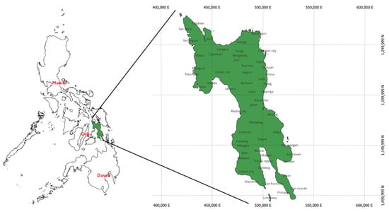
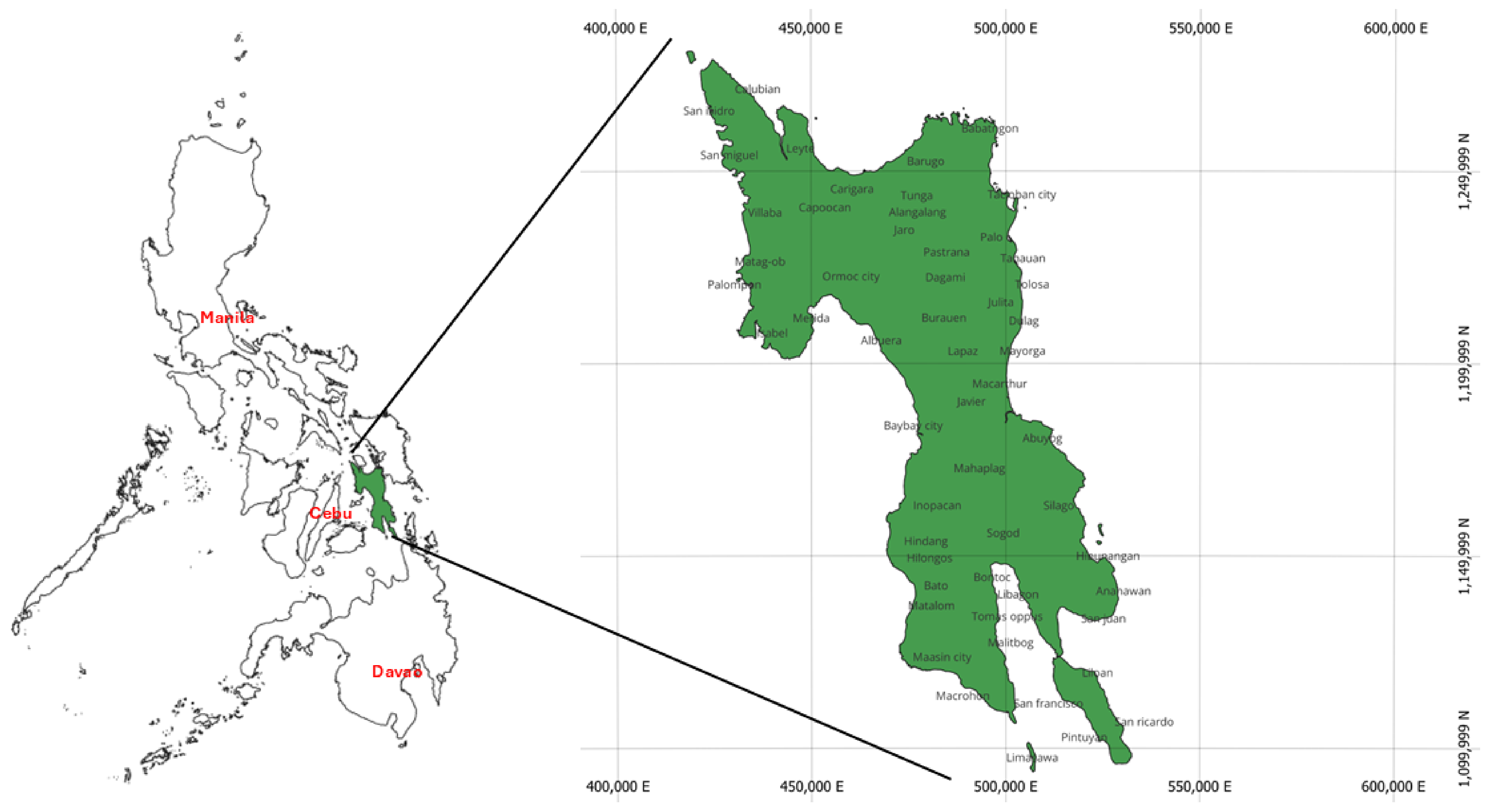
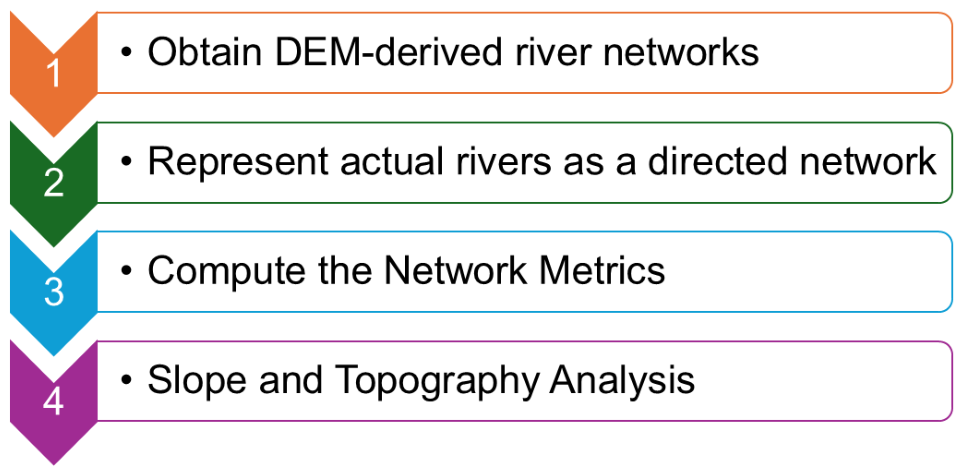
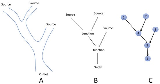
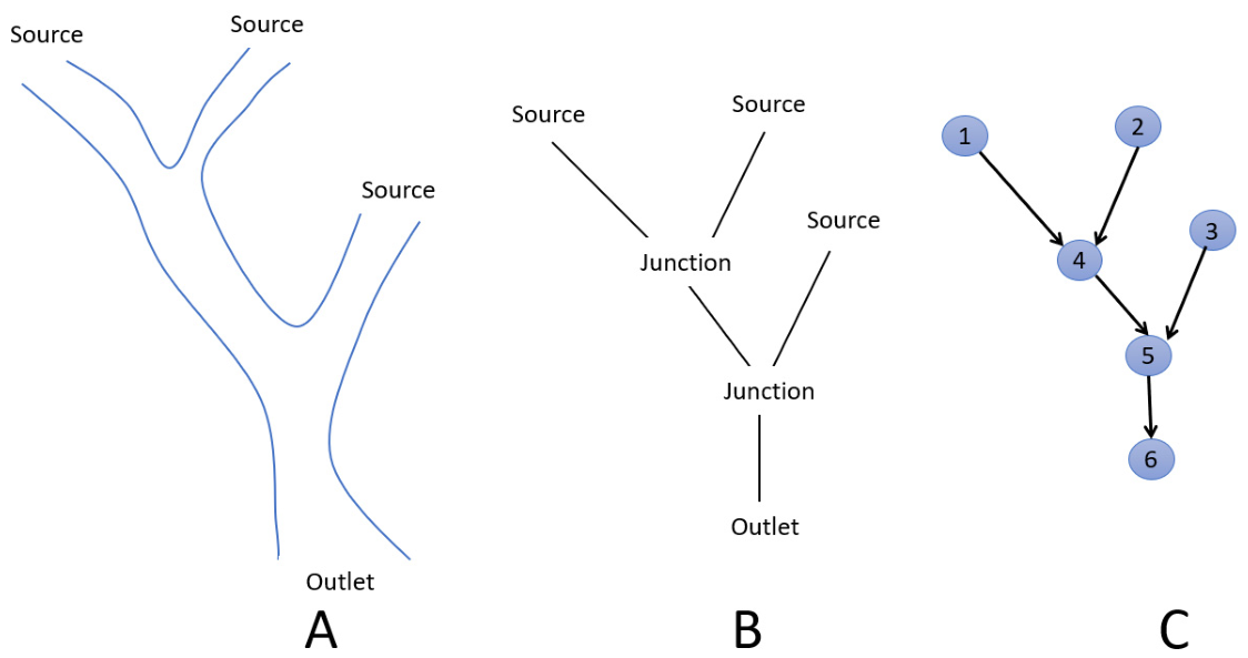
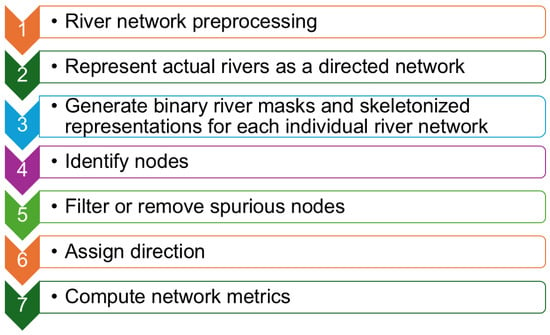
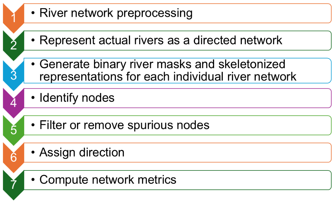
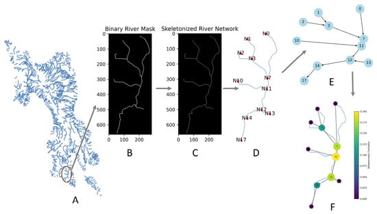
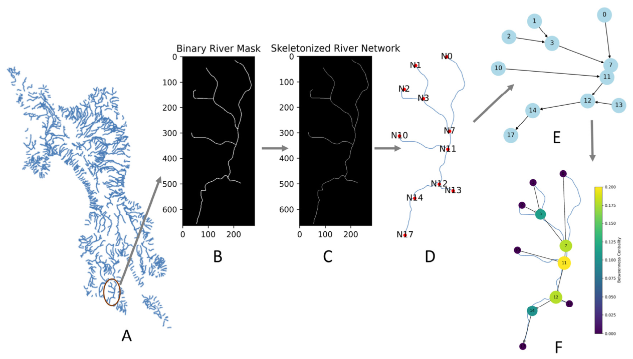
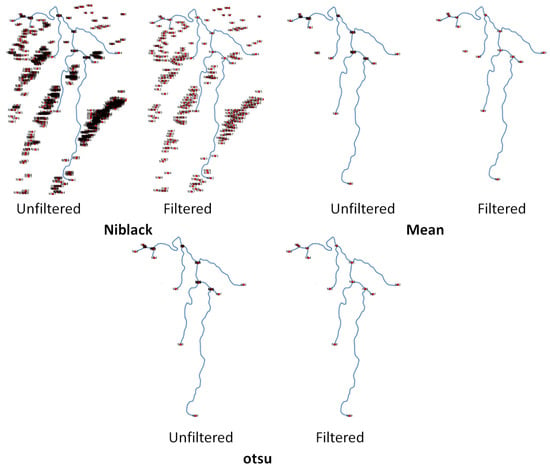
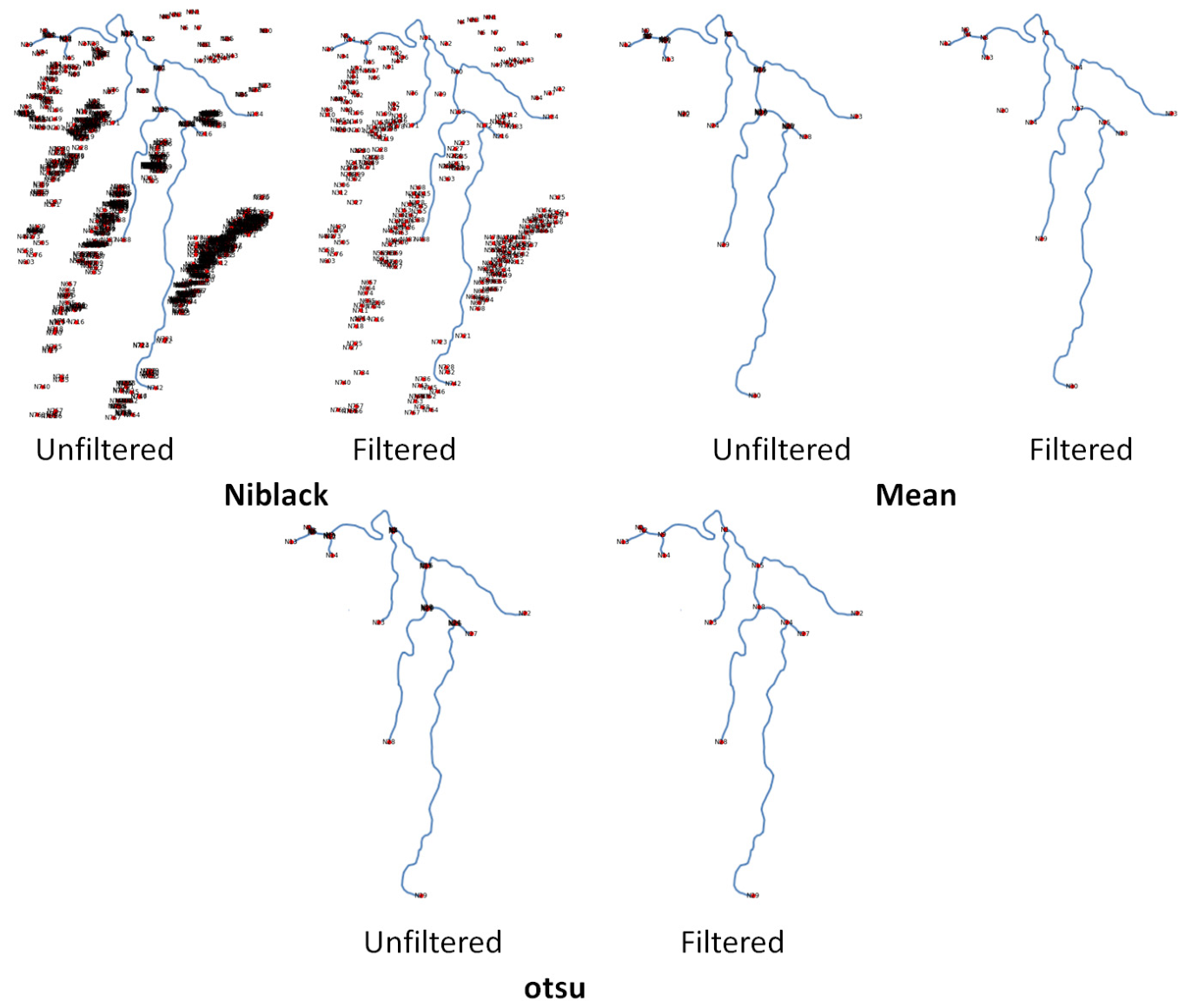
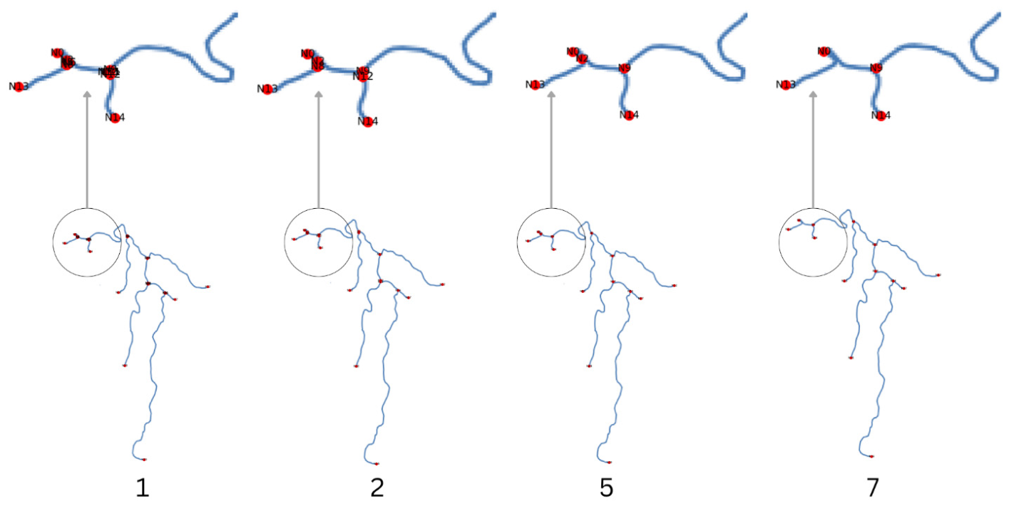
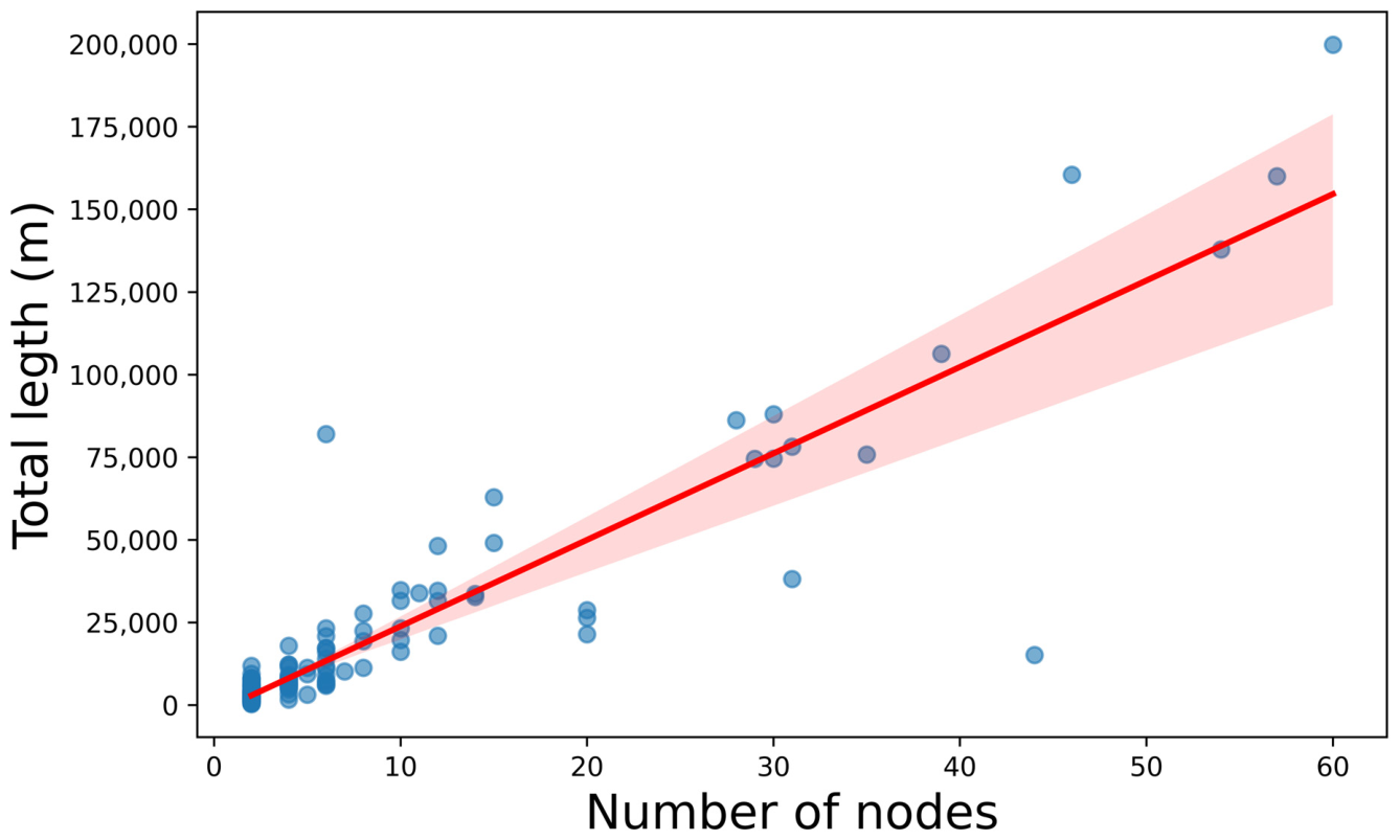
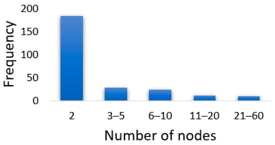
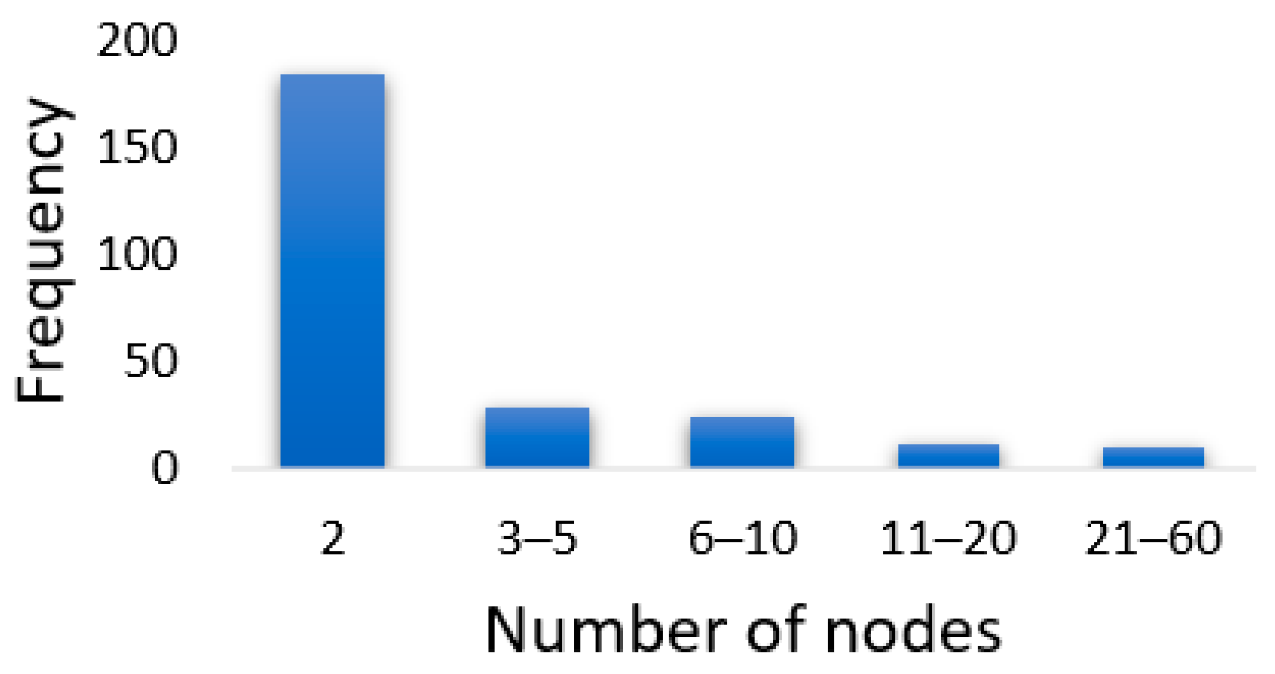
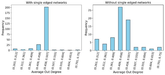
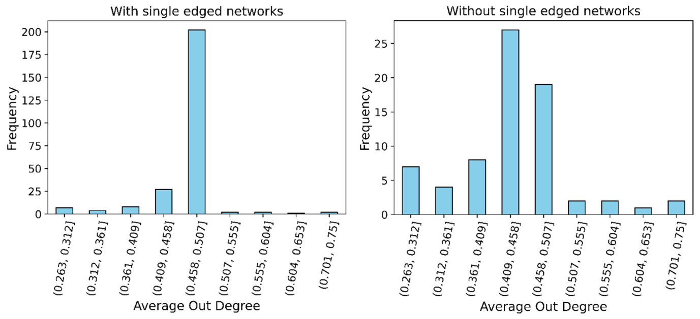
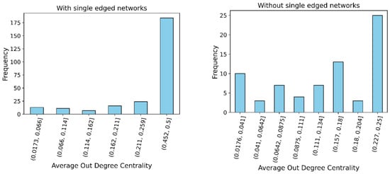
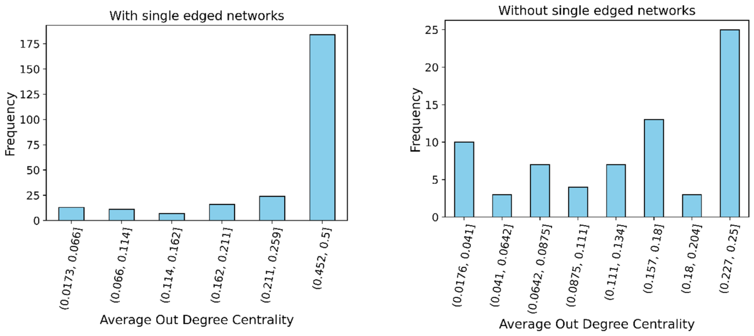
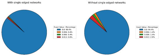
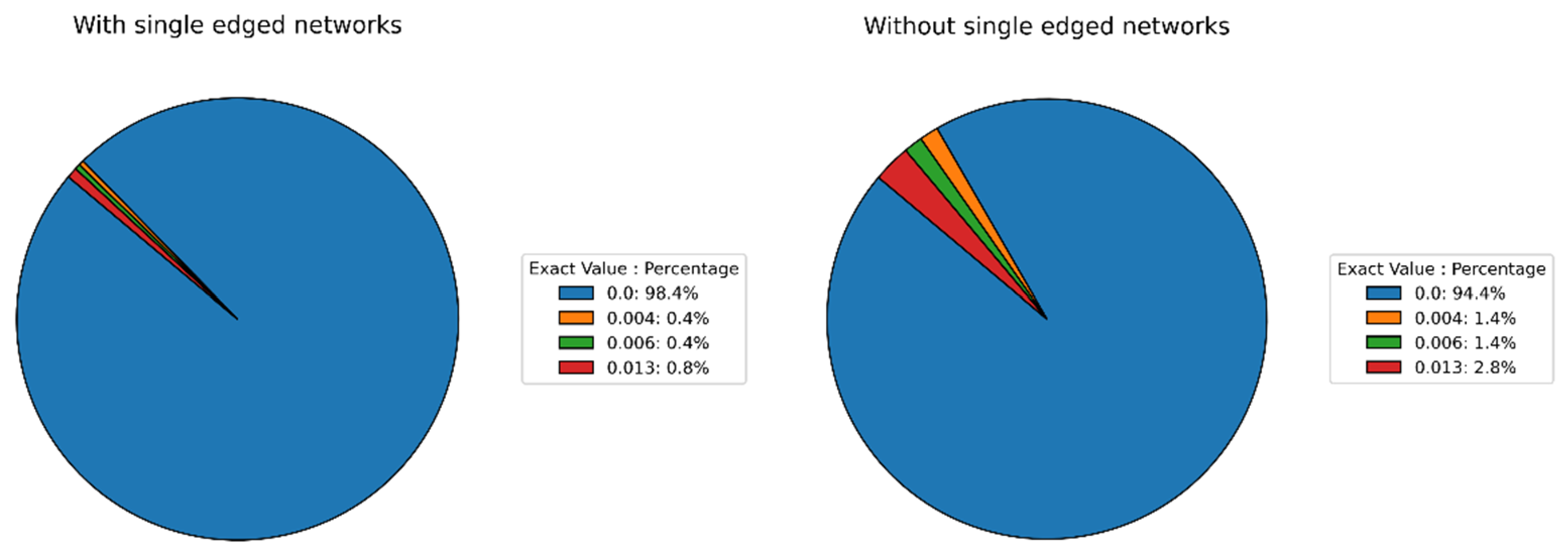
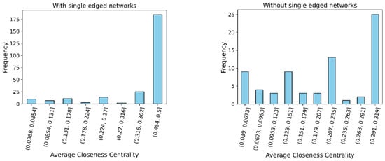
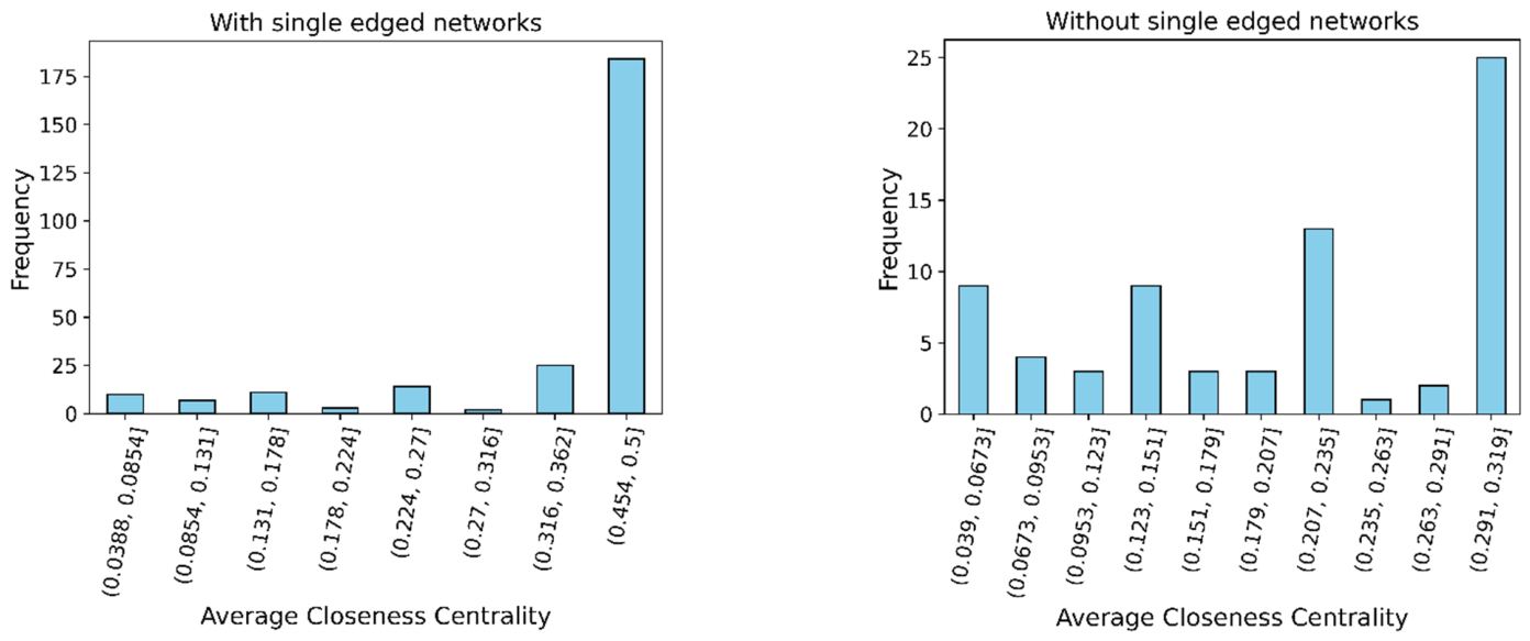
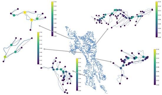
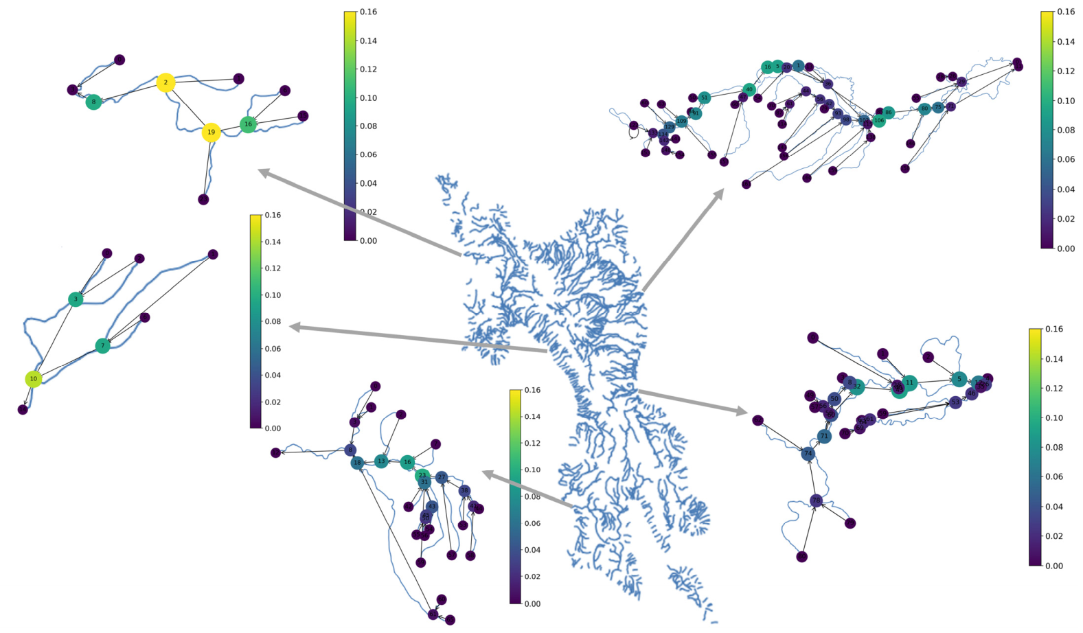
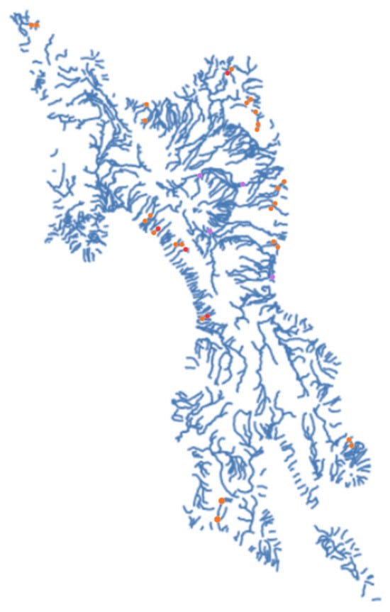
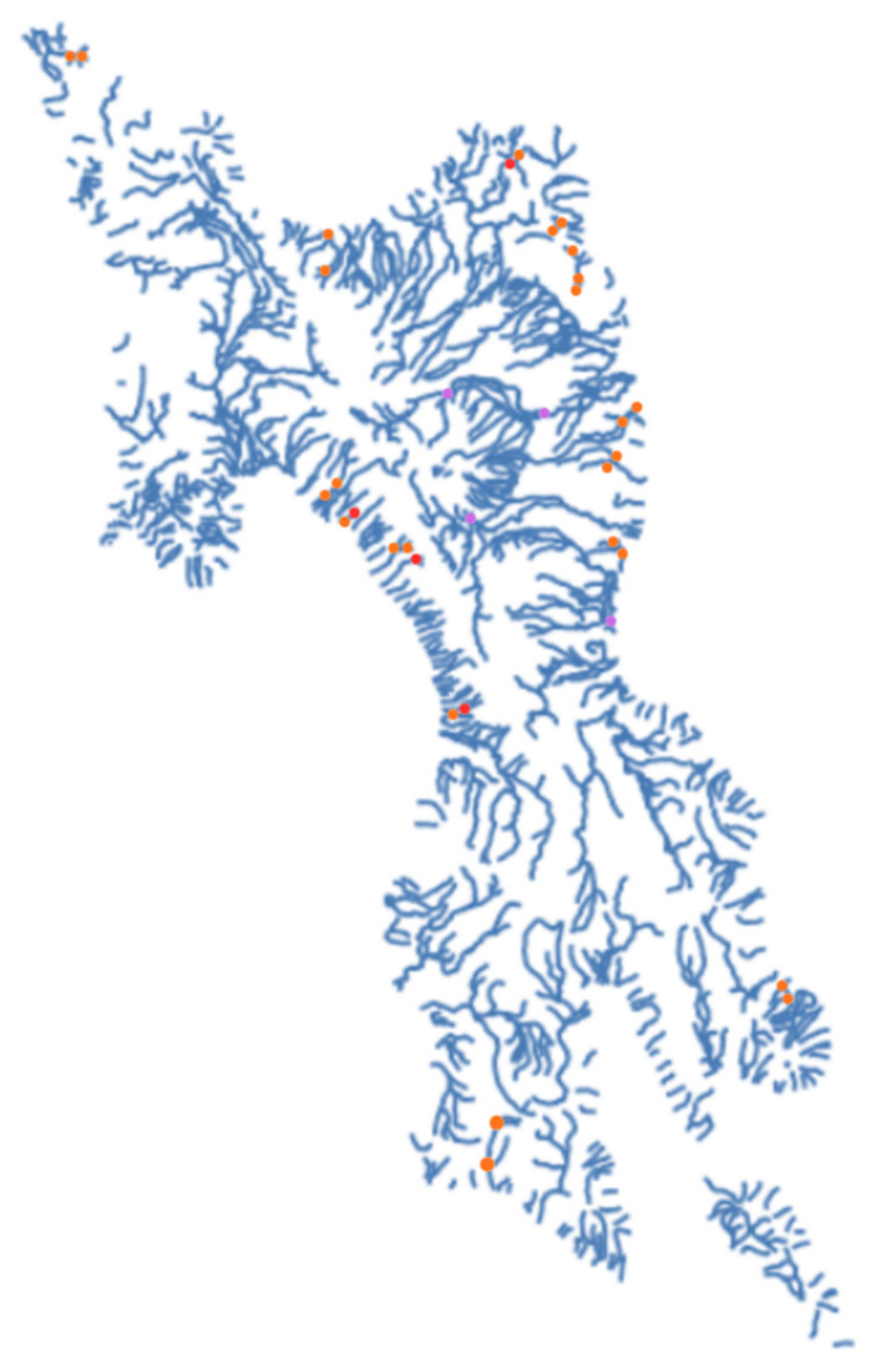
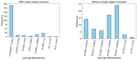
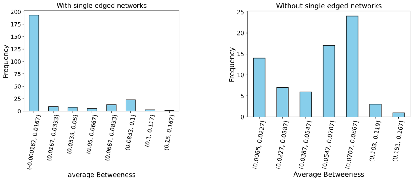
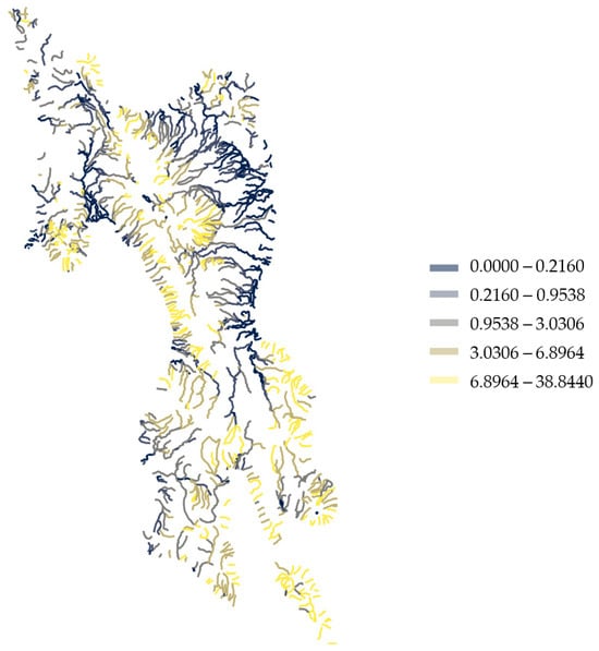
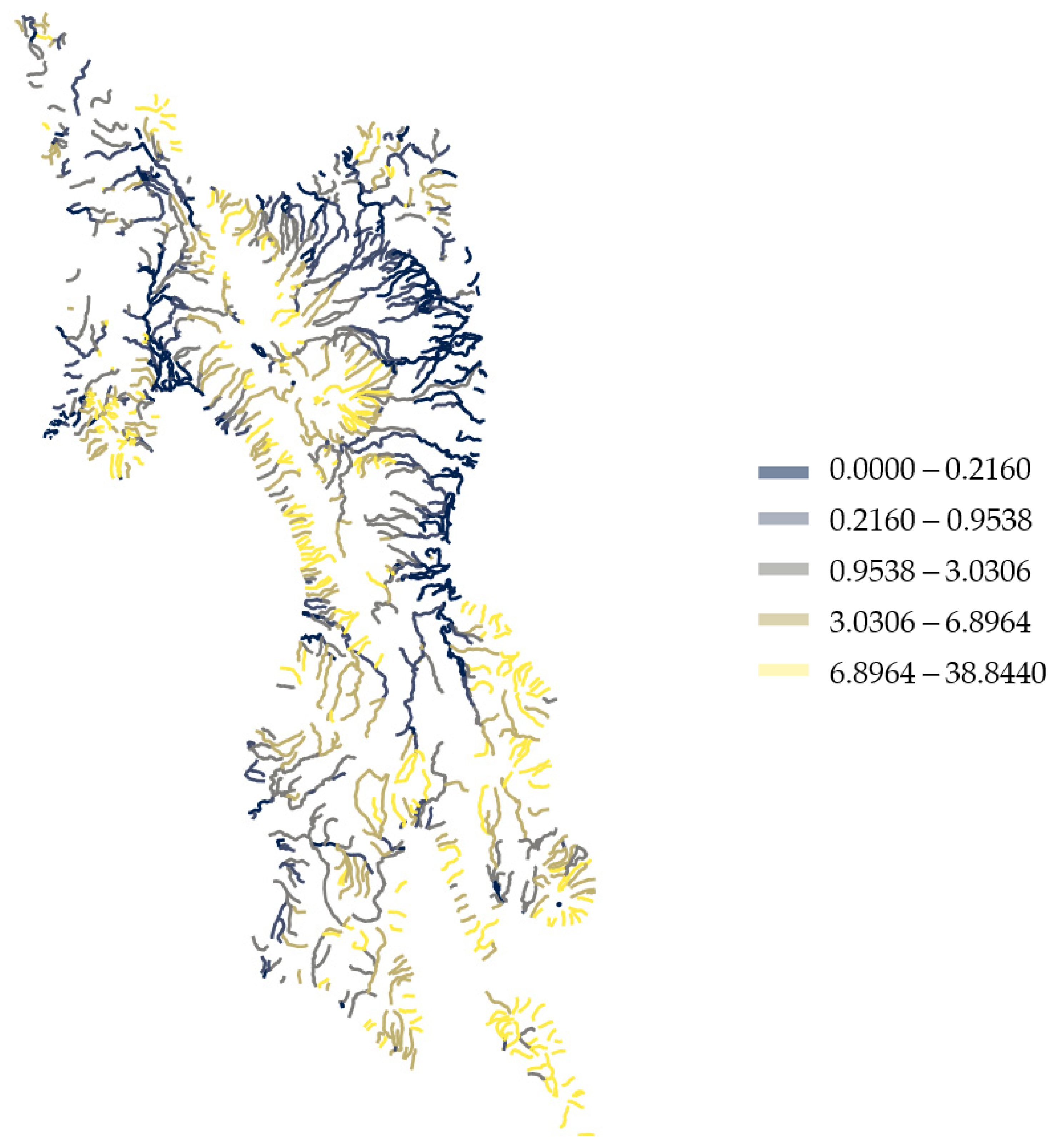
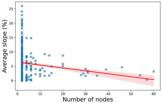
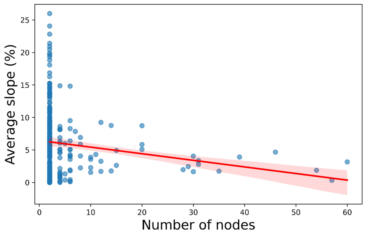

Disclaimer/Publisher’s Note: The statements, opinions and data contained in all publications are solely those of the individual author(s) and contributor(s) and not of MDPI and/or the editor(s). MDPI and/or the editor(s) disclaim responsibility for any injury to people or property resulting from any ideas, methods, instructions or products referred to in the content. |
© 2026 by the authors. Licensee MDPI, Basel, Switzerland. This article is an open access article distributed under the terms and conditions of the Creative Commons Attribution (CC BY) license.