A New Quantile Differential Family with an Explicit Quadratic Distribution: Theory, Statistical Properties, and Applications

Abstract

Quantile functions provide a natural representation of probability distributions and offer direct advantages for random variate generation, simulation, and quantile-based statistical analysis. In this paper, we develop a quantile-differential construction in which a probability model is characterized through a differential equation satisfied directly by its quantile function. Within this framework, we introduce a one-parameter continuous model, termed the quadratic quantile distribution (QQD), whose explicit quantile representation leads to a simple and analytically tractable probability model. Closed-form expressions are obtained for the cumulative distribution function, probability density function, survival function, hazard rate, and cumulative hazard function. Several structural properties are also investigated, including shape characteristics, stochastic ordering, entropy measures, fractional moments, and quantile-based descriptive measures. Particular attention is devoted to the upper-tail behavior. The survival function is regularly varying with index $-1$, so that the QQD has a Pareto-type tail with tail index one. Consequently, the ordinary mean is infinite, whereas fractional moments exist only for orders less than one. This feature makes quantile-, survival-, and tail-based summaries more appropriate than conventional moment-based descriptions. Maximum likelihood estimation is developed for the model parameter, and its finite-sample behavior is examined through an extensive Monte Carlo study. The simulation results show a progressive reduction in bias, root mean squared error, and mean absolute error as the sample size increases, providing numerical evidence consistent with the expected large-sample behavior of the estimator without treating simulation as a proof of asymptotic consistency. The empirical performance of the QQD is examined using three right-skewed datasets from reliability and biomedical applications. Comparisons with established one- and two-parameter distributions show that the QQD can provide a competitive likelihood-based fit while retaining the simplicity of a single unknown parameter. Graphical comparisons further complement the numerical criteria, particularly in assessing the behavior of the fitted models in the upper tail. Overall, the results suggest that the QQD offers a parsimonious and analytically convenient alternative for selected strongly right-skewed positive data, while its suitability should be assessed on a case-by-case basis in view of its heavy-tailed structure.

1. Introduction

Probability distributions form a fundamental part of statistical modeling and play an important role in reliability engineering, actuarial science, economics, finance, environmental studies, biomedical research, and many other scientific areas. Since the pioneering work of Pearson [1], a wide range of continuous distributions has been developed to accommodate the variety of shapes and tail behaviors encountered in real data. Classical treatments of continuous distributions can be found in Johnson and Kotz [2]. Nevertheless, the increasing complexity of modern datasets continues to motivate the search for models that combine flexibility with analytical simplicity.

One important line of research has focused on generator-based methods for constructing new families of distributions. Representative examples include the Marshall–Olkin family [3], the beta-generated family [4], the T–X family of Alzaatreh et al. [5], and the quantile-based T–X construction introduced by Aljarrah et al. [6]. These approaches have considerably enlarged the range of available probability models and provide useful mechanisms for introducing additional shape flexibility. At the same time, repeated transformations or additional parameters may lead to increasingly complicated distributional forms. This has encouraged the development of alternative constructions in which tractability and interpretability remain central considerations.

A natural possibility is to work directly with the quantile function. Unlike a density or distribution function, the quantile function gives a complete description of a continuous distribution while offering several practical advantages. An explicit quantile representation facilitates random variate generation, supports robust quantile-based summaries, and may simplify the study of distributional characteristics that are less easily accessible from the density alone. Early contributions to quantile-function modeling include the work of Parzen [7], while a comprehensive treatment is given by Gilchrist [8]. More recently, quantile-based methods have received renewed attention in statistical modeling and data analysis, as illustrated by Redivo et al. [9].

Several probability models have consequently been developed directly through explicit quantile representations. Examples include the quantile model of Sankaran et al. [10], the quantile-based flattened logistic distribution of Sharma and Chakrabarty [11], its subsequent generalization [12], and the reduced quantile-function family introduced by Chukwuma et al. [13]. These contributions demonstrate that the quantile function itself can serve as a useful starting point for distributional modeling rather than being recovered only after a density or cumulative distribution function has been specified.

In parallel, considerable attention has been given to parsimonious lifetime distributions that can describe positively skewed observations without introducing a large number of parameters. Examples include the XLindley distribution [14], reliability extensions of the Zeghdoudi distribution [15], the quadratic exponential distribution [16], and other recent continuous models with useful analytical and practical properties [17]. Such developments reflect the continuing need for simple models that retain sufficient flexibility for reliability and lifetime data.

The present work adopts a complementary quantile-based viewpoint. Instead of specifying the quantile only through a direct parametric formula, we consider it as the solution of a first-order differential equation of the form

$$Q^{\prime }\left(u\right)=\mathrm{\Psi }(u,Q\left(u\right)),0<u<1.$$

Here, the function $\mathrm{\Psi }$ governs the local evolution of the quantile curve. This formulation creates a direct connection between ordinary differential equations and probability modeling and provides a convenient way to study monotonicity and other structural features of the resulting quantile function. Although differential equations are well established in many areas of applied mathematics, their direct use as a mechanism for generating quantile functions appears to have received comparatively limited attention in the literature on distribution construction.

We refer to this constructive mechanism as a quantile differential family (QDF). Positivity of the differential generator alone is not sufficient to guarantee a valid probability model. Accordingly, the framework is formulated under regularity conditions ensuring existence, uniqueness, continuation of the solution on $(0,1)$, strict monotonicity, and appropriate endpoint behavior. Under these conditions, the solution can serve as an admissible quantile function, from which the corresponding distribution and density functions can be recovered. The QDF is therefore intended as a constructive quantile-based methodology rather than as a replacement for existing distribution-generating families.

As a concrete illustration, we introduce the quadratic quantile distribution (QQD), a one-parameter continuous model with quantile function

$$Q(u;\theta )=\theta {\displaystyle \frac{u(2-u)}{1-u}},0<u<1,\theta >0.$$

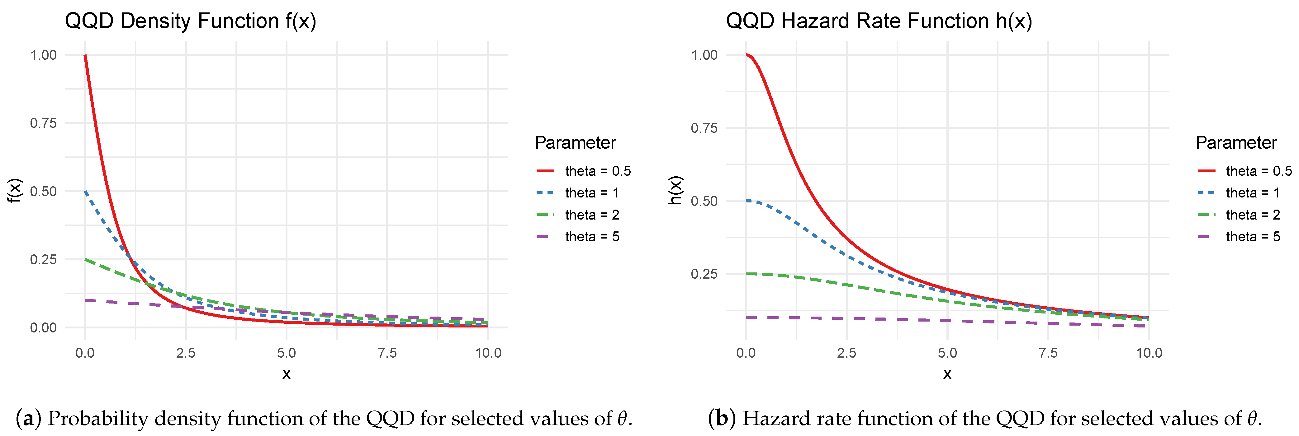
The model admits explicit expressions for its cumulative distribution function, density, survival function, hazard rate, and cumulative hazard function. It has a strictly decreasing density and hazard rate, while $\theta$ acts as a scale parameter. A distinctive feature of the QQD is its Pareto-type upper tail:

$$\overline{F}\left(x\right)\sim {\displaystyle \frac{\theta }{x}},x\to \infty .$$

Consequently, the distribution has tail index one and does not possess a finite ordinary mean. This makes quantiles, survival probabilities, exceedance probabilities, and other tail-oriented summaries particularly relevant for its interpretation.

Statistical inference for the QQD is developed through maximum likelihood estimation. The finite-sample behavior of the estimator is examined by Monte Carlo simulation, with attention to bias, root mean squared error, mean absolute error, and sampling variability. These numerical experiments are used to assess finite-sample performance and are not interpreted as a proof of asymptotic consistency.

The practical performance of the QQD is further examined using three right-skewed datasets from reliability and biomedical applications, namely, Kevlar failure times, aircraft failure intervals, and bladder-cancer remission times. Comparisons are made with several established one- and two-parameter distributions using likelihood-based information criteria and graphical diagnostics. The aim is not to claim universal superiority but rather to examine whether the QQD can provide a competitive and parsimonious description of selected strongly right-skewed positive data while retaining the simplicity of a single unknown parameter.

The remainder of the paper is organized as follows. Section 2 introduces the quantile-differential construction, states the admissibility conditions, and derives the QQD together with its principal distributional and reliability functions. Section 3 studies the main mathematical properties of the model, including its upper-tail behavior, fractional moments, transform properties, entropy measures, stochastic ordering, and quantile-based descriptive measures. Section 4 develops maximum likelihood inference and presents the Monte Carlo study. Section 5 investigates the empirical performance of the QQD using three real datasets and compares it with established competing models. Finally, Section 6 summarizes the main findings, discusses the limitations of the model, and outlines possible directions for further research.

2. Quantile Differential Construction of the Proposed Distribution

This section presents the quantile-differential construction used to define the proposed quadratic quantile distribution (QQD). Rather than starting from a probability density or cumulative distribution function, the construction takes the quantile function as the primary modeling object and characterizes it through a first-order differential equation. We first specify the conditions under which such an equation yields an admissible quantile function and then introduce the QQD as an explicit illustration of this approach.

2.1. The Quantile Differential Construction

Let X be a continuous random variable with cumulative distribution function F and quantile function

$$Q\left(u\right)=F^{-1}\left(u\right),0<u<1.$$

We consider a first-order initial-value problem of the form

$$Q^{\prime }\left(u\right)=\mathrm{\Psi }(u,Q\left(u\right)),Q\left(u_0\right)=q_0,u_0\in (0,1),$$

(1)

where

$$\mathrm{\Psi }:(0,1)\times \mathbb{R}⟶(0,\infty )$$

is referred to as the quantile differential generator.

Positivity of $\mathrm{\Psi }$ ensures monotonicity of a solution but by itself does not guarantee its existence, uniqueness, or continuation over the whole interval $(0,1)$. We therefore call a generator $\mathrm{\Psi }$ admissible when the following conditions are satisfied:

(A1)

$\mathrm{\Psi }(u,x)$ is continuous on $(0,1)\times \mathbb{R}$ and $\mathrm{\Psi }(u,x)>0$.

(A2)

For every compact interval $I\subset (0,1)$, $\mathrm{\Psi }$ is locally Lipschitz continuous in its second argument, uniformly with respect to $u\in I$.

(A3)

For every compact interval $I\subset (0,1)$, there exist constants $a_I,b_I>0$ such that

$$\left|\mathrm{\Psi }(u,x)\right|\le a_I+b_I\left|x\right|,(u,x)\in I\times \mathbb{R}.$$

(A4)

The resulting solution possesses endpoint limits

$$q_{-}=\underset{u\downarrow 0}{\lim }Q\left(u\right),q_{+}=\underset{u\uparrow 1}{\lim }Q\left(u\right),$$

with

$$-\infty \le q_{-}<q_{+}\le +\infty .$$

Under conditions (A1)–(A3), standard existence and uniqueness results for ordinary differential equations ensure that the solution of (1) is uniquely continued throughout $(0,1)$. Moreover, because $\mathrm{\Psi }>0$,

$$Q^{\prime }\left(u\right)>0,0<u<1,$$

so that Q is strictly increasing. Together with condition (A4), this allows Q to serve as the quantile function of a continuous distribution supported on $(q_{-},q_{+})$. We use the term quantile differential family (QDF) for distributions obtained through admissible quantile-differential constructions of this type.

The basic link between the quantile differential equation and the corresponding probability density is summarized by the following standard identity.

Lemma 1.

Let Q be an admissible quantile function satisfying (1). Then,

$$f\left(Q\left(u\right)\right)={\displaystyle \frac{1}{Q^{\prime }\left(u\right)}}={\displaystyle \frac{1}{\mathrm{\Psi }(u,Q(u\left)\right)}},0<u<1.$$

Equivalently,

$$f\left(x\right)={\displaystyle \frac{1}{\mathrm{\Psi }\left(F\right(x),x)}}.$$

Indeed, the result follows immediately by differentiating the identity $F\left(Q\right(u\left)\right)=u$. Thus, once an admissible quantile solution is known, its density can be recovered directly without introducing an additional distribution-generating transformation.

2.2. Construction of the Quadratic Quantile Distribution

We now consider an explicit one-parameter quantile function that provides a simple illustration of the preceding construction. For $\theta >0$, define

$$Q\left(u\right)=\theta {\displaystyle \frac{u(2-u)}{1-u}},0<u<1.$$

(2)

Differentiating (2) correctly gives

$$\begin{array}{c}\hfill Q^{\prime }\left(u\right)=\theta {\displaystyle \frac{u^2-2u+2}{{(1-u)}^2}}=\theta \left[1+{\displaystyle \frac{1}{{(1-u)}^2}}\right],0<u<1.\end{array}$$

(3)

Since

$$u^2-2u+2={(1-u)}^2+1>0,$$

we have $Q^{\prime }\left(u\right)>0$ throughout $(0,1)$. The corresponding differential generator may therefore be written as

$$\begin{array}{c}\hfill {\mathrm{\Psi }}_{\theta }(u,x)=\theta {\displaystyle \frac{u^2-2u+2}{{(1-u)}^2}},0<u<1,\end{array}$$

(4)

which, in this particular example, does not depend explicitly on x. It is continuous and positive on $(0,1)$ and is trivially locally Lipschitz in its second argument. Moreover,

$$\begin{array}{c}\hfill {\displaystyle \underset{u\downarrow 0}{\lim }}Q\left(u\right)=0,{\displaystyle \underset{u\uparrow 1}{\lim }}Q\left(u\right)=+\infty .\end{array}$$

Consequently, (2) defines a continuous probability distribution on $(0,\infty )$, which we call the quadratic quantile distribution, denoted by $X\sim \mathrm{QQD}\left(\theta \right)$.

Distribution and Reliability Functions

To obtain the cumulative distribution function, set $x=Q\left(u\right)$ in (2). This gives

$$\theta u^2-(x+2\theta )u+x=0.$$

The root belonging to $(0,1)$ is

$$F\left(x\right)={\displaystyle \frac{x+2\theta -\sqrt{x^2+4{\theta }^2}}{2\theta }},x\ge 0.$$

(5)

Differentiating (5) yields the probability density function

$$f\left(x\right)={\displaystyle \frac{\sqrt{x^2+4{\theta }^2}-x}{2\theta \sqrt{x^2+4{\theta }^2}}},x\ge 0.$$

(6)

For numerical and analytical purposes, the equivalent form

$$\begin{array}{c}\hfill f\left(x\right)={\displaystyle \frac{2\theta }{\sqrt{x^2+4{\theta }^2}\left(x+\sqrt{x^2+4{\theta }^2}\right)}}\end{array}$$

(7)

is sometimes more convenient. As a consistency check, substituting $x=Q\left(u\right)$ into (6) gives

$$f\left(Q\left(u\right)\right)={\displaystyle \frac{1}{Q^{\prime }\left(u\right)}},$$

in agreement with Lemma  1.

The survival function is

$$S\left(x\right)=1-F\left(x\right)={\displaystyle \frac{\sqrt{x^2+4{\theta }^2}-x}{2\theta }},x\ge 0.$$

(8)

Rationalizing the numerator gives the useful equivalent representation

$$\begin{array}{c}\hfill S\left(x\right)={\displaystyle \frac{2\theta }{x+\sqrt{x^2+4{\theta }^2}}},x\ge 0.\end{array}$$

(9)

This form will be particularly useful in Section 3 when examining the upper-tail behavior of the model.

Combining Equations (6) and (8), the hazard rate is

$$h\left(x\right)={\displaystyle \frac{f\left(x\right)}{S\left(x\right)}}={\displaystyle \frac{1}{\sqrt{x^2+4{\theta }^2}}},x\ge 0.$$

(10)

Accordingly, the cumulative hazard function takes the convenient form

$$\begin{array}{c}\hfill H\left(x\right)=-\log S\left(x\right)=\log \left({\displaystyle \frac{x+\sqrt{x^2+4{\theta }^2}}{2\theta }}\right),x\ge 0.\end{array}$$

(11)

Thus, despite being defined through a quantile differential equation, the QQD retains explicit expressions for all of its principal distributional and reliability functions. This tractability is useful both for theoretical analysis and for likelihood-based inference.

2.3. Basic Shape Characteristics

Only the main shape features needed to interpret the model are recorded here; further analytical properties are developed in Section 3. From (6),

$$\begin{array}{c}\hfill f^{\prime }\left(x\right)=-{\displaystyle \frac{2\theta }{{(x^2+4{\theta }^2)}^{3/2}}}<0,x>0,\end{array}$$

so the density is strictly decreasing and attains its maximum at the left endpoint $x=0$. Similarly,

$$\begin{array}{c}\hfill h^{\prime }\left(x\right)=-{\displaystyle \frac{x}{{(x^2+4{\theta }^2)}^{3/2}}}<0,x>0,\end{array}$$

showing that the QQD has a decreasing failure rate. In addition,

$$Q(u;\theta )=\theta Q(u;1),$$

so $\theta$ acts as a scale parameter: increasing $\theta$ stretches the distribution while preserving its basic shape.

Figure 1 illustrates these features for $\theta =0.5,1,2,$ and 5. As $\theta$ increases, the density spreads over a wider range, whereas the hazard function remains decreasing for all parameter values.

3. Mathematical Properties of the Quadratic Quantile Distribution

The explicit quantile representation of the QQD makes it possible to study several properties that are particularly relevant for heavy-tailed data. Since the basic distributional and shape characteristics were established in Section 2, we focus here on the upper-tail behavior, moment existence, information measures, stochastic ordering, and quantile-based descriptive measures. This organization avoids repeating elementary consequences of the distribution and density functions.

3.1. Tail Behavior, Moments, and Transform Properties

The upper-tail behavior is one of the most distinctive features of the QQD. Using the rationalized form of the survival function obtained in Section 2,

$$S\left(x\right)={\displaystyle \frac{2\theta }{x+\sqrt{x^2+4{\theta }^2}}},x\ge 0,$$

its asymptotic behavior follows directly.

Theorem 1

(Tail behavior). Let $X\sim \mathrm{QQD}\left(\theta \right)$, $\theta >0$. Then,

$$S\left(x\right)\sim {\displaystyle \frac{\theta }{x}},x\to \infty .$$

Consequently, the survival function is regularly varying at infinity with index $-1$, and the QQD has a Pareto-type upper tail with tail index one.

Proof. 

From the rationalized survival function,

$$xS\left(x\right)={\displaystyle \frac{2\theta }{1+\sqrt{1+4{\theta }^2/x^2}}}.$$

Hence,

$$\underset{x\to \infty }{\lim }xS\left(x\right)={\displaystyle \frac{2\theta }{1+1}}=\theta ,$$

which proves that

$$S\left(x\right)\sim {\displaystyle \frac{\theta }{x}}.$$

The regular variation property follows immediately:

$$\underset{x\to \infty }{\lim }{\displaystyle \frac{S\left(cx\right)}{S\left(x\right)}}={\displaystyle \frac{1}{c}},c>0.$$

   □

The preceding result has an important consequence for moment existence. In particular, the ordinary mean is infinite. More generally, an exact expression can be obtained for the fractional moments that do exist.

Proposition 1

(Fractional moments). For $-1<r<1$,

$$\mathbb{E}\left(X^r\right)={\displaystyle \frac{{\theta }^r}{2}}B\left({\displaystyle \frac{1-r}{2}},r+1\right),$$

where $B(·,·)$ denotes the beta function. In contrast,

$$\mathbb{E}\left(X^r\right)=\infty ,r\ge 1.$$

In particular,

$$\mathbb{E}\left(X\right)=\infty .$$

Proof. 

Using the quantile representation,

$$\mathbb{E}\left(X^r\right)={\int }_0^{1}Q{\left(u\right)}^{r}du.$$

Setting $t=1-u$ gives

$$Q\left(u\right)=\theta {\displaystyle \frac{1-t^2}{t}},$$

and therefore,

$$\mathbb{E}\left(X^r\right)={\theta }^r{\int }_0^1{t}^{-r}{(1-t^2)}^{r}dt.$$

With $y=t^2$,

$$\mathbb{E}\left(X^r\right)={\displaystyle \frac{{\theta }^r}{2}}{\int }_0^1{y}^{(1-r)/2-1}{(1-y)}^{r}dy,$$

which yields

$$\mathbb{E}\left(X^r\right)={\displaystyle \frac{{\theta }^r}{2}}B\left({\displaystyle \frac{1-r}{2}},r+1\right).$$

The beta integral is finite precisely for $-1<r<1$. For $r\ge 1$, divergence also follows from the Pareto-type tail established in Theorem 1.    □

Remark 1.

The QQD therefore does not possess a moment generating function in the usual sense. Indeed,

$$M_X\left(t\right)=\mathbb{E}\left(e^{tX}\right)=\infty ,t>0.$$

For $t<0$, the quantity $\mathbb{E}\left(e^{tX}\right)$ is finite and corresponds to the Laplace transform evaluated at $-t$. Thus, Laplace- or quantile-based summaries are more appropriate than an MGF-based description for this heavy-tailed model.

The infinite mean should be kept in mind when the QQD is applied to insurance losses, rainfall extremes, network latencies, and related positive data. In such settings, the model is primarily intended to describe distributional shape and upper-tail behavior; quantiles, survival probabilities, and exceedance measures are therefore more informative than moment-based summaries.

3.2. Shannon Entropy

The Shannon entropy can be derived conveniently from the quantile density. For a continuously differentiable and strictly increasing quantile function,

$$\mathcal{H}\left(X\right)={\int }_0^1\log Q^{\prime }\left(u\right)du.$$

Theorem 2

(Shannon entropy). Let $X\sim \mathrm{QQD}\left(\theta \right)$, $\theta >0$. Then,

$$\begin{array}{|c|}\hline \mathcal{H}\left(X\right)=\log \left(2\theta \right)+{\displaystyle \frac{\pi }{2}}.\\ \hline\end{array}$$

Proof. 

From Section 2,

$$Q^{\prime }\left(u\right)=\theta \left[1+{\displaystyle \frac{1}{{(1-u)}^2}}\right].$$

Setting $t=1-u$ gives

$$\begin{array}{cc}\hfill \mathcal{H}\left(X\right)& =\log \theta +{\int }_0^1\log \left({\displaystyle \frac{1+t^2}{t^2}}\right)dt\hfill \\ & =\log \theta +{\int }_0^1\log (1+t^2)dt-2{\int }_0^1\log tdt.\hfill \end{array}$$

Using

$${\int }_0^1\log tdt=-1$$

and

$${\int }_0^1\log (1+t^2)dt=\log 2-2+{\displaystyle \frac{\pi }{2}},$$

we obtain

$$\mathcal{H}\left(X\right)=\log \left(2\theta \right)+{\displaystyle \frac{\pi }{2}}.$$

   □

3.3. Rényi Entropy

For $\gamma >0$, $\gamma \ne 1$, the Rényi entropy of order $\gamma$ is defined by

$${\mathcal{R}}_{\gamma }\left(X\right)={\displaystyle \frac{1}{1-\gamma }}\log \left({\int }_0^{\infty }f{\left(x\right)}^{\gamma }dx\right).$$

Proposition 2

(Rényi entropy). Let $X\sim \mathrm{QQD}\left(\theta \right)$ and let

$$\gamma >{\displaystyle \frac{1}{2}},\gamma \ne 1.$$

Then,

$$\begin{array}{|c|}\hline {\mathcal{R}}_{\gamma }\left(X\right)=\log \theta +{\displaystyle \frac{1}{1-\gamma }}\log \left[{\displaystyle \frac{{}_{2}F_1\left(\gamma -\frac{1}{2},\gamma -1;\gamma +\frac{1}{2};-1\right)}{2\gamma -1}}\right],\\ \hline\end{array}$$

where ${}_{2}F_1$ denotes the Gauss hypergeometric function.

Proof. 

Using $x=Q\left(u\right)$ and

$$f\left(Q\left(u\right)\right)={\displaystyle \frac{1}{Q^{\prime }\left(u\right)}},$$

we have

$${\int }_0^{\infty }f{\left(x\right)}^{\gamma }dx={\int }_0^1{Q}^{\prime }{\left(u\right)}^{1-\gamma }du.$$

With $t=1-u$ and

$$Q^{\prime }\left(u\right)=\theta {\displaystyle \frac{1+t^2}{t^2}},$$

this becomes

$${\int }_0^{\infty }f{\left(x\right)}^{\gamma }dx={\theta }^{1-\gamma }{\int }_0^1{t}^{2\gamma -2}{(1+t^2)}^{1-\gamma }dt.$$

The integral converges when $\gamma >1/2$ and admits the representation

$${\int }_0^1{t}^{2\gamma -2}{(1+t^2)}^{1-\gamma }dt={\displaystyle \frac{1}{2\gamma -1}}{}_{2}F_1\left(\gamma -{\displaystyle \frac{1}{2}},\gamma -1;\gamma +{\displaystyle \frac{1}{2}};-1\right).$$

Substitution into the definition of Rényi entropy gives the stated result.    □

The Shannon entropy is recovered in the limiting case:

$$\underset{\gamma \to 1}{\lim }{\mathcal{R}}_{\gamma }\left(X\right)=\log \left(2\theta \right)+{\displaystyle \frac{\pi }{2}},$$

in agreement with Theorem 2. No separate proof is needed here.

3.4. Stochastic Ordering

Since $\theta$ acts as a scale parameter, the stochastic ordering of two QQD variables follows directly from their quantile functions.

Proposition 3.

Let

$$X_1\sim \mathrm{QQD}\left({\theta }_1\right),X_2\sim \mathrm{QQD}\left({\theta }_2\right),$$

with

$$0<{\theta }_1<{\theta }_2.$$

Then,

$$X_1{\le }_{\mathrm{st}}{X}_2.$$

Equivalently,

$$F_1\left(x\right)\ge F_2\left(x\right),x\ge 0,$$

or

$$S_1\left(x\right)\le S_2\left(x\right),x\ge 0.$$

Proof. 

For every $u\in (0,1)$,

$$Q_i\left(u\right)={\theta }_i{\displaystyle \frac{u(2-u)}{1-u}},i=1,2.$$

Since

$${\displaystyle \frac{u(2-u)}{1-u}}>0,$$

the inequality ${\theta }_1<{\theta }_2$ implies

$$Q_1\left(u\right)<Q_2\left(u\right),0<u<1.$$

The standard quantile characterization of the usual stochastic order therefore yields

$$X_1{\le }_{\mathrm{st}}{X}_2.$$

   □

Thus, increasing $\theta$ shifts the distribution toward larger values without changing its basic shape, confirming its interpretation as a scale parameter.

3.5. Quantile-Based Descriptive Measures

Because the QQD has an infinite first moment, conventional moment-based summaries such as the coefficient of variation and moment-based skewness are not appropriate. Quantile-based measures provide natural and robust alternatives.

Using the quantile function already given in Section 2, the first quartile, median, and third quartile are

$$Q_1={\displaystyle \frac{7}{12}}\theta ,Q_2={\displaystyle \frac{3}{2}}\theta ,Q_3={\displaystyle \frac{15}{4}}\theta .$$

Hence, the median is

$$\begin{array}{|c|}\hline Med\left(X\right)={\displaystyle \frac{3}{2}}\theta ,\\ \hline\end{array}$$

while the interquartile range is

$$\begin{array}{|c|}\hline IQR\left(X\right)=Q_3-Q_1={\displaystyle \frac{19}{6}}\theta .\\ \hline\end{array}$$

Bowley’s quartile coefficient of skewness [18] is defined by

$$B={\displaystyle \frac{Q_3+Q_1-2Q_2}{Q_3-Q_1}}.$$

For the QQD,

$$\begin{array}{|c|}\hline B={\displaystyle \frac{8}{19}}\approx 0.4211.\\ \hline\end{array}$$

The positive value of B confirms the right-skewed character of the QQD. Unlike conventional moment-based skewness, Bowley’s coefficient remains well defined despite the non-existence of the ordinary mean and higher moments.

4. Maximum Likelihood Estimation and Monte Carlo Study

This section develops maximum likelihood estimation for the parameter $\theta$ and examines its finite-sample behavior by Monte Carlo simulation. The explicit quantile representation of the QQD is particularly convenient for this purpose, since random samples can be generated directly without numerical inversion or acceptance–rejection procedures.

4.1. Maximum Likelihood Estimation

Let

$$X_1,X_2,\dots ,X_n$$

be a random sample from $\mathrm{QQD}\left(\theta \right)$, with $\theta >0$. From Section 2, the density can be written in the numerically convenient form

$$f(x;\theta )={\displaystyle \frac{2\theta }{\sqrt{x^2+4{\theta }^2}\left(x+\sqrt{x^2+4{\theta }^2}\right)}},x>0.$$

For notational simplicity, define

$$r_i\left(\theta \right)=\sqrt{x_i^2+4{\theta }^2},i=1,\dots ,n.$$

The likelihood function is

$$L\left(\theta \right)={\displaystyle \prod _{i=1}^n}{\displaystyle \frac{2\theta }{r_i\left(\theta \right)\{r_i\left(\theta \right)+x_i\}}},$$

and the corresponding log-likelihood is

$$\ell \left(\theta \right)=n\log \left(2\theta \right)-{\displaystyle \sum _{i=1}^n}\log r_i\left(\theta \right)-{\displaystyle \sum _{i=1}^n}\log \left\{r_i\left(\theta \right)+x_i\right\}.$$

(12)

Differentiating (12) gives the score function

$$U\left(\theta \right)={\displaystyle \frac{n}{\theta }}-4\theta {\displaystyle \sum _{i=1}^n}\left[{\displaystyle \frac{1}{r_i{\left(\theta \right)}^2}}+{\displaystyle \frac{1}{r_i\left(\theta \right)\{r_i\left(\theta \right)+x_i\}}}\right].$$

(13)

The maximum likelihood estimator $\widehat{\theta }$ is therefore obtained as the positive solution of

$$U(\widehat{\theta })=0,$$

or, equivalently, by direct numerical maximization of (12). Since no simple closed-form solution is available, numerical optimization is used throughout the study.

To ensure the positivity constraint automatically, we optimize with respect to

$$\eta =\log \theta ,\theta =e^{\eta },$$

using the BFGS algorithm implemented in the optim() function in R. The estimate on the original scale is then recovered as

$$\widehat{\theta }=e^{\widehat{\eta }}.$$

For reference, the Fisher information in one observation is

$$I_1\left(\theta \right)={\displaystyle \frac{1}{{\theta }^2}}\left({\displaystyle \frac{\pi }{4}}-{\displaystyle \frac{1}{3}}\right),$$

(14)

so that

$$I_n\left(\theta \right)={\displaystyle \frac{n}{{\theta }^2}}\left({\displaystyle \frac{\pi }{4}}-{\displaystyle \frac{1}{3}}\right).$$

Under the usual regularity conditions for maximum likelihood estimation, this gives the large-sample approximation

$$\sqrt{n}\left(\widehat{\theta }-\theta \right)\stackrel{d}{⟶}N\left(0,{\displaystyle \frac{{\theta }^2}{\frac{\pi }{4}-\frac{1}{3}}}\right).$$

Accordingly, an approximate standard error is

$$se\left(\widehat{\theta }\right)\approx {\displaystyle \frac{\widehat{\theta }}{\sqrt{n\left(\frac{\pi }{4}-\frac{1}{3}\right)}}}.$$

The Monte Carlo experiment below is intended to assess the finite-sample behavior of the estimator and should not be interpreted as a proof of these asymptotic properties.

4.2. Simulation Design and Performance Measures

Random observations are generated directly from the QQD quantile function. Specifically, if

$$U\sim \mathcal{U}(0,1),$$

then

$$X=Q\left(U\right)=\theta {\displaystyle \frac{U(2-U)}{1-U}}$$

(15)

has the $\mathrm{QQD}\left(\theta \right)$ distribution.

The simulation considers four representative parameter values,

$$\theta \in \{0.5,1,2,5\},$$

and five sample sizes,

$$n\in \{20,50,100,200,500\}.$$

For each combination of $\theta$ and n, $N=5000$ independent samples are generated, and the parameter is estimated by maximum likelihood.

Let ${\widehat{\theta }}_j$ denote the estimate obtained from the jth replication. The finite-sample performance is summarized by the empirical mean

$$\overline{\widehat{\theta }}={\displaystyle \frac{1}{N}}{\displaystyle \sum _{j=1}^N}{\widehat{\theta }}_j,$$

the empirical bias

$$Bias={\displaystyle \frac{1}{N}}{\displaystyle \sum _{j=1}^N}\left({\widehat{\theta }}_j-\theta \right),$$

the mean absolute error

$$MAE={\displaystyle \frac{1}{N}}{\displaystyle \sum _{j=1}^N}\left|{\widehat{\theta }}_j-\theta \right|,$$

and the root mean squared error

$$RMSE={\left[{\displaystyle \frac{1}{N}}{\displaystyle \sum _{j=1}^N}{\left({\widehat{\theta }}_j-\theta \right)}^2\right]}^{1/2}.$$

These measures describe complementary aspects of finite-sample performance: the empirical mean and bias assess systematic estimation error, whereas the MAE and RMSE quantify overall estimation accuracy.

4.3. Monte Carlo Results

The Monte Carlo results are summarized in

Table 1. Monte Carlo performance of the maximum likelihood estimator of $\theta$ for the QQD based on $N=5000$ replications.

$\mathit{\theta }$	n	Mean	Bias	RMSE	MAE
$0.5$	20	0.52836	0.02836	0.18918	0.14043
	50	0.51305	0.01305	0.11192	0.08627
	100	0.50568	0.00568	0.07552	0.05944
	200	0.50266	0.00266	0.05096	0.04066
	500	0.50107	0.00107	0.03326	0.02651
1	20	1.05012	0.05012	0.36684	0.27535
	50	1.02176	0.02176	0.22044	0.17190
	100	1.00993	0.00993	0.15117	0.11876
	200	1.00503	0.00503	0.10696	0.08478
	500	1.00438	0.00438	0.06658	0.05259
2	20	2.11117	0.11117	0.73989	0.55049
	50	2.03396	0.03396	0.43508	0.33864
	100	2.02727	0.02727	0.30595	0.23859
	200	2.00889	0.00889	0.21420	0.17009
	500	2.00251	0.00251	0.13474	0.10728
5	20	5.30414	0.30414	1.85032	1.37455
	50	5.10720	0.10720	1.09024	0.84311
	100	5.05994	0.05994	0.75264	0.58848
	200	5.02577	0.02577	0.53231	0.42267
	500	5.00990	0.00990	0.33342	0.26482

. For each configuration, $N=5000$ independent samples were generated using the explicit QQD quantile function. The same simulation design was used for

$$\theta \in \{0.5,1,2,5\},n\in \{20,50,100,200,500\}.$$

To ensure reproducibility, the random-number generator was initialized with the fixed seed 20260904.

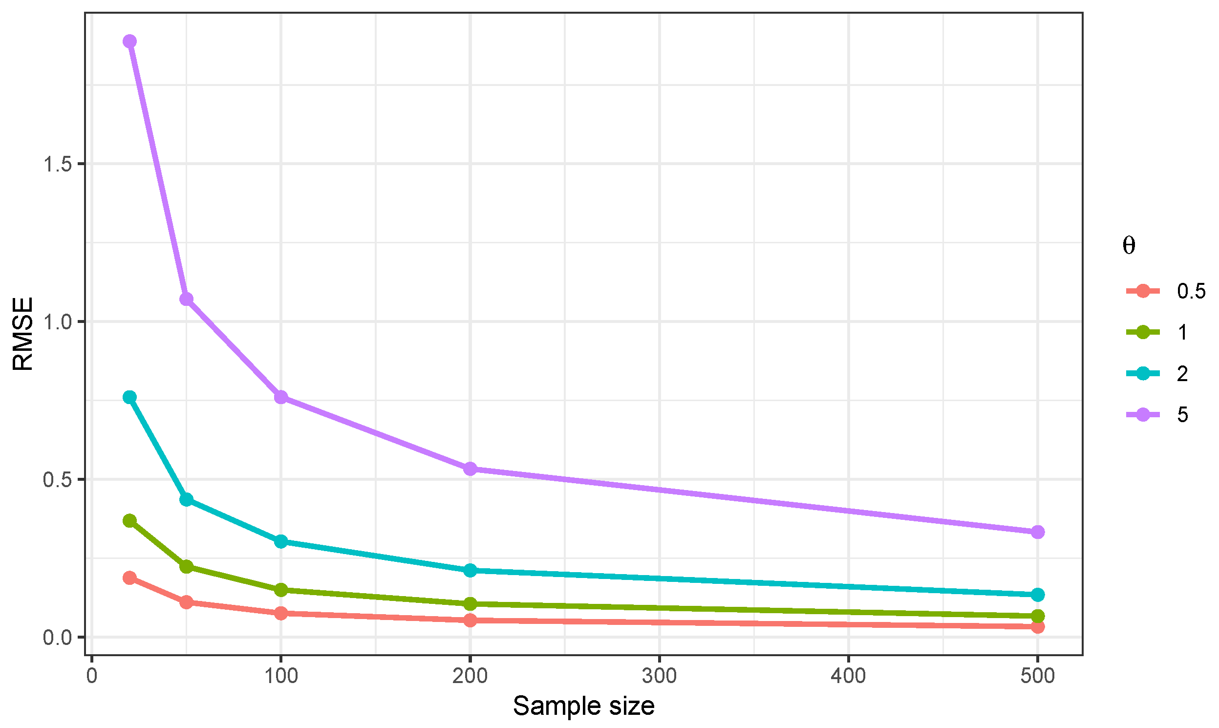
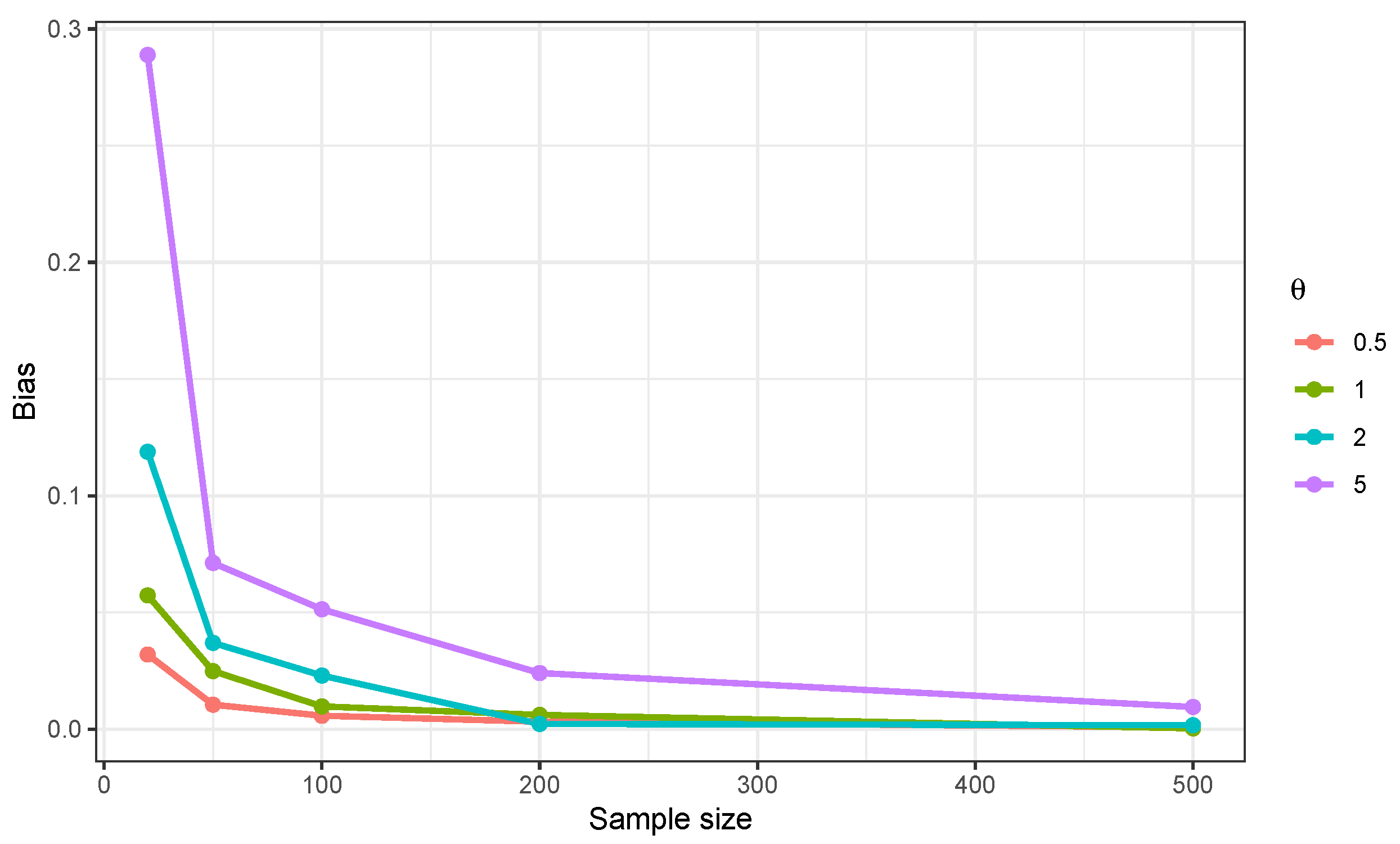
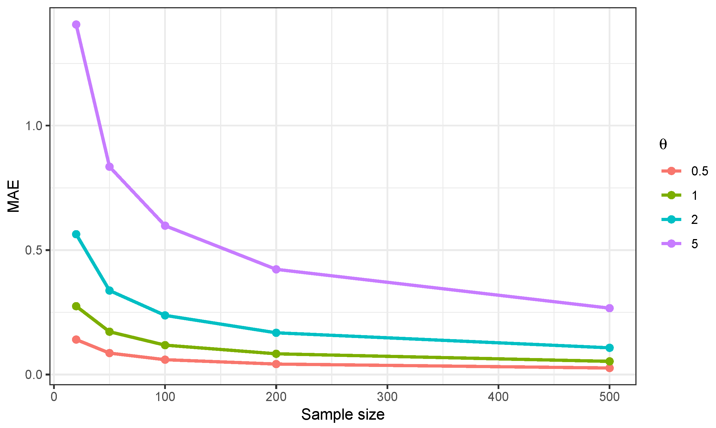
Table 1 shows a clear improvement in estimation accuracy as the sample size increases. For all four values of $\theta$, the empirical mean moves closer to the true parameter value, while the bias, RMSE, and MAE decrease substantially with increasing n.

For example, when $\theta =0.5$, the bias decreases from $0.02836$ at $n=20$ to $0.00107$ at $n=500$. Over the same range of sample sizes, the RMSE decreases from $0.18918$ to $0.03326$, and the MAE decreases from $0.14043$ to $0.02651$. A similar pattern is observed for the other parameter values.

When $\theta =1$, the RMSE decreases from $0.36684$ at $n=20$ to $0.06658$ at $n=500$, whereas for $\theta =2$, it decreases from $0.73989$ to $0.13474$. For $\theta =5$, the corresponding reduction is from $1.85032$ to $0.33342$. Thus, although the absolute estimation error increases with the magnitude of $\theta$, the overall pattern is similar across the four settings. This is consistent with the role of $\theta$ as a scale parameter.

A small positive finite-sample bias is visible, particularly for $n=20$, but it becomes substantially smaller for moderate and large sample sizes. The simultaneous decrease in bias, RMSE, and MAE indicates that the maximum likelihood estimates become increasingly concentrated around the true parameter value as more observations are available.

These findings provide numerical evidence of satisfactory finite-sample performance and are consistent with the expected large-sample behavior of the maximum likelihood estimator. As emphasized earlier, however, the Monte Carlo experiment is intended to assess finite-sample performance and should not be interpreted as a mathematical proof of consistency.

4.4. Graphical Assessment

The finite-sample behavior of the maximum likelihood estimator is further examined through Figure 2, Figure 3, Figure 4, Figure 5 and Figure 6. These graphical summaries complement the numerical results reported in Table 1 and illustrate the evolution of bias, estimation error, and sampling variability as the sample size increases.

Figure 2, Figure 3 and Figure 4 show a systematic reduction in bias, RMSE, and MAE as the sample size increases. This pattern is observed across all considered parameter values and is consistent with the numerical results in Table 1.

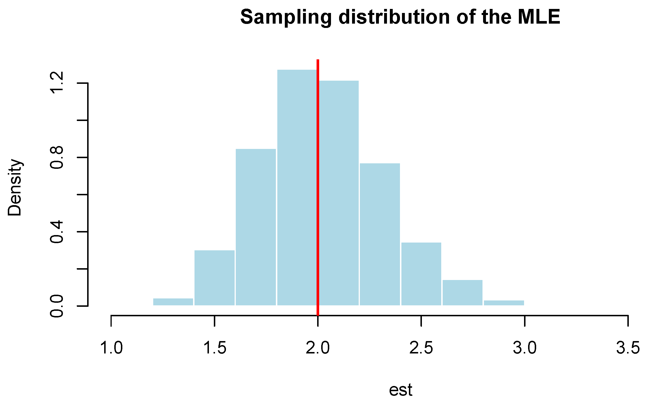
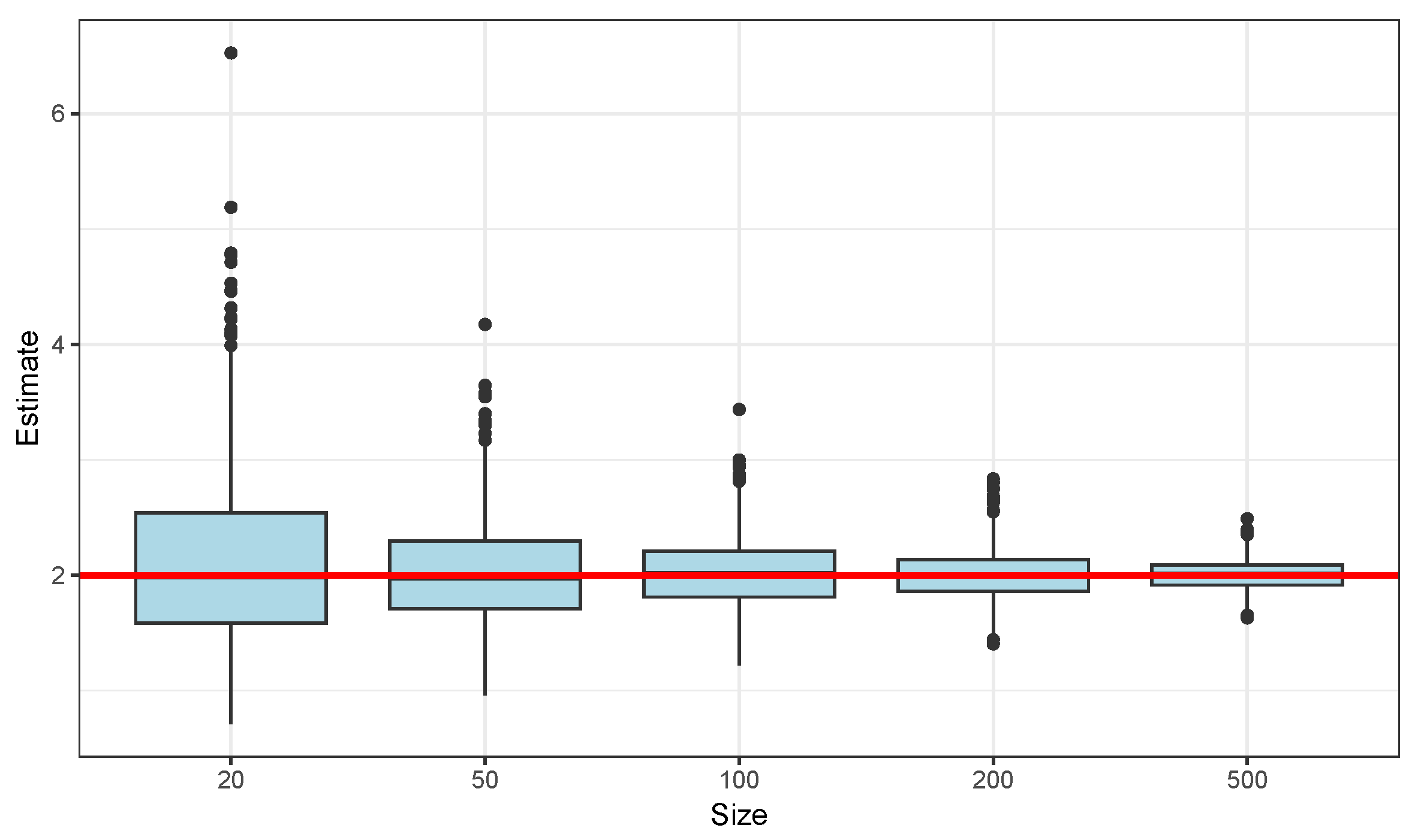
Figure 5 shows that for $\theta =2$ and $n=100$, the sampling distribution of $\widehat{\theta }$ is centered close to the true parameter value and is approximately symmetric. Likewise, Figure 6 illustrates the progressive reduction in sampling dispersion as n increases, while the median remains close to the generating value.

Taken together, the graphical and numerical results indicate that the maximum likelihood estimates become increasingly accurate and concentrated around the true parameter value as the sample size grows. These findings provide numerical evidence consistent with the expected large-sample behavior of the estimator.

5. Applications

To complement the theoretical results and the Monte Carlo study, we examine the empirical performance of the proposed one-parameter quadratic quantile distribution (QQD) using three positive datasets from reliability and biomedical studies. The first concerns failure times of Kevlar 373/Epoxy specimens, a dataset widely used in lifetime and reliability modeling [19,20]. The second consists of aircraft air-conditioning failure intervals originally considered by Proschan [21], while the third contains bladder-cancer remission times reported in the survival-analysis literature [22]. These datasets display different degrees of positive skewness and upper-tail variability and therefore provide useful settings for assessing the practical behavior of the QQD.

Throughout the applications, the QQD is fitted using exactly the one-parameter formulation developed in Section 2, Section 3 and Section 4,

$$Q(u;\theta )=\theta {\displaystyle \frac{u(2-u)}{1-u}},0<u<1,\theta >0,$$

so that only the parameter $\theta$ is estimated.

To place the QQD in a reasonably broad empirical context, we consider both classical and more recent lifetime distributions. The classical benchmarks include the Exponential, Gamma, Log-normal, Inverse Gaussian, Half-normal, Rayleigh, and Maxwell distributions [23], together with the Weibull [24], Lomax [25], and generalized Exponential [26] models. The one-parameter comparisons also include the Lindley distribution [27,28], XLindley [14], New XLindley [29], Q-Lindley [30], Shanker [31], Xgamma [32], Akash [33], Sujatha [34], Ishita [35], Pranav [36], and the Length-biased Lindley distribution [37]. For the extended one-parameter comparisons, the Aradhana [38], Amarendra [39], and Rama [40] distributions are also considered.

All unknown parameters are estimated by maximum likelihood. Model comparison is based on the maximized log-likelihood together with the Akaike information criterion (AIC) [41], its small-sample correction AICc [42], the Bayesian information criterion (BIC) [43], the Hannan–Quinn information criterion (HQIC) [44], and the consistent Akaike information criterion (CAIC) [45]. Specifically,

$$\mathrm{AIC}=-2\ell \left(\widehat{\mathsf{\eta }}\right)+2k,$$

$$\mathrm{AICc}=\mathrm{AIC}+{\displaystyle \frac{2k(k+1)}{n-k-1}},$$

$$\mathrm{BIC}=-2\ell \left(\widehat{\mathsf{\eta }}\right)+k\log n,$$

$$\mathrm{HQIC}=-2\ell \left(\widehat{\mathsf{\eta }}\right)+2k\log \left(\log n\right),$$

and

$$\mathrm{CAIC}=-2\ell \left(\widehat{\mathsf{\eta }}\right)+k(\log n+1),$$

where $\widehat{\mathsf{\eta }}$ denotes the vector of maximum likelihood estimates and k denotes the number of estimated parameters. Larger maximized log-likelihood values and smaller information-criterion values indicate a more favorable likelihood-based fit.

The first application uses a relatively broad comparison involving both one- and two-parameter distributions. The aircraft and bladder-cancer applications focus mainly on selected one-parameter competitors, which allows the QQD to be compared with models of the same dimensionality. Accordingly, the corresponding tables should be interpreted as within-class comparisons rather than exhaustive rankings of every model examined during the numerical analysis.

A distinctive feature of the QQD is its Pareto-type upper tail,

$$\overline{F}\left(x\right)\sim {\displaystyle \frac{\theta }{x}},x\to \infty .$$

Thus, the distribution has tail index one and does not possess a finite ordinary mean. This property is relevant when interpreting the real-data examples: the QQD is more naturally assessed through its distributional shape, quantiles, survival and exceedance probabilities, and upper-tail behavior than through mean-based summaries. The purpose of these applications is therefore not to establish universal dominance but to examine whether a simple one-parameter model with an explicit quantile representation can provide a competitive and parsimonious description of strongly right-skewed positive data.

5.1. Kevlar 373/Epoxy Failure-Time Data

The first application considers a sample of $n=60$ Kevlar 373/Epoxy failure times. The observations are positive and strongly right-skewed, with a relatively large concentration of short failure times and a smaller number of substantially larger observations. This feature makes the dataset particularly informative for assessing a distribution such as the QQD, which combines a decreasing density with a slowly decaying upper tail.

A broad benchmark comparison is considered in this application. In addition to the QQD, eleven one-parameter distributions are fitted: Exponential, Lindley, XLindley, New XLindley, QLindley, Shanker, Xgamma, Akash, Ishita, Sujatha, and Pranav. Seven two-parameter alternatives are also included: Weibull, Gamma, Log-normal, Lomax, Inverse Gaussian, generalized Exponential, and Gompertz [46].

Table 2. Likelihood-based comparison for the Kevlar 373/Epoxy failure-time data ($n=60$). The best likelihood/information-criterion values are shown in bold.

Model	k	LogL	AIC	AICc	BIC	HQIC	CAIC
QQD	1	$-\mathbf{46}.\mathbf{43}$	$\mathbf{94}.\mathbf{85}$	$\mathbf{94}.\mathbf{92}$	$\mathbf{96}.\mathbf{95}$	$\mathbf{95}.\mathbf{67}$	$\mathbf{97}.\mathbf{95}$
Lomax	2	$-47.08$	98.16	98.37	102.35	99.80	104.35
Inverse Gaussian	2	$-47.92$	99.83	100.04	104.02	101.47	106.02
Weibull	2	$-52.02$	108.04	108.25	112.23	109.68	114.23
Gamma	2	$-54.53$	113.07	113.28	117.25	114.71	119.25
Gen. Exponential	2	$-55.03$	114.05	114.26	118.24	115.69	120.24
Exponential	1	$-56.91$	115.83	115.90	117.92	116.65	118.92
Gompertz	2	$-56.92$	117.84	118.05	122.03	119.48	124.03
Log-normal	2	$-57.22$	118.44	118.65	122.63	120.08	124.63
XLindley	1	$-58.48$	118.96	119.03	121.06	119.78	122.06
Pranav	1	$-58.56$	119.12	119.19	121.22	119.94	122.22
Ishita	1	$-59.83$	121.67	121.74	123.76	122.49	124.76
Shanker	1	$-60.78$	123.57	123.64	125.66	124.39	126.66
Xgamma	1	$-62.10$	126.20	126.27	128.29	127.02	129.29
Lindley	1	$-62.24$	126.48	126.55	128.57	127.30	129.57
Akash	1	$-62.97$	127.95	128.02	130.04	128.77	131.04
New XLindley	1	$-64.30$	130.60	130.67	132.70	131.42	133.70
Sujatha	1	$-65.97$	133.93	134.00	136.03	134.75	137.03
QLindley	1	$-66.84$	135.68	135.75	137.77	136.50	138.77

reports the maximized log-likelihood and the five information criteria for all fitted models.

The results in Table 2 are consistently favorable to the QQD for this dataset. The proposed model attains the largest maximized log-likelihood, $\log L=-46.43$, as well as the smallest values of all five information criteria:

$$\mathrm{AIC}=94.85,\mathrm{AICc}=94.92,\mathrm{BIC}=96.95,$$

$$\mathrm{HQIC}=95.67,\mathrm{CAIC}=97.95.$$

Thus, the preference for the QQD is not specific to a single penalty criterion.

The closest competitor is the two-parameter Lomax distribution, with $\log L=-47.08$, AIC $=98.16$, AICc $=98.37$, BIC $=102.35$, HQIC $=99.80$, and CAIC $=104.35$. In particular,

$$\mathsf{\Delta }\mathrm{AIC}=98.16-94.85=3.31,$$

whereas

$$\mathsf{\Delta }\mathrm{BIC}=102.35-96.95=5.40.$$

The likelihoods of the two models are relatively close, but the additional Lomax parameter leads to a larger penalty under each information criterion.

The Inverse Gaussian distribution is the next closest alternative, with AIC $=99.83$ and BIC $=104.02$. The Weibull, Gamma, generalized Exponential, Gompertz, and Log-normal models produce appreciably larger information-criterion values.

The comparison with models of equal complexity is more pronounced. Among the competing one-parameter distributions, the Exponential model has the next smallest AIC, equal to $115.83$, which is approximately $20.98$ units larger than that of the QQD. The XLindley and Pranav models yield AIC values of $118.96$ and $119.12$, respectively, while the remaining Lindley-type alternatives give still larger values.

These results suggest that the QQD provides a particularly favorable combination of likelihood fit and parsimony for this sample. Its slowly decaying upper tail may help accommodate the small number of large observations without introducing a second shape parameter. Nevertheless, this conclusion is dataset-specific and should not be interpreted as evidence that the QQD will dominate competing lifetime models in general.

5.2. Aircraft Failure-Time Data

The second application considers $n=30$ aircraft failure intervals. The observations are strongly right-skewed, with a substantial concentration of relatively short failure intervals accompanied by a small number of considerably larger observations. Such a pattern provides a useful setting for examining the ability of the QQD to represent positive reliability data with pronounced upper-tail variability.

For this application, we present a focused comparison with selected one-parameter lifetime distributions. The comparison includes the New XLindley, Half-normal, XLindley, Lindley, Shanker, Xgamma, Sujatha, Length-biased Lindley, Akash, Ishita, Rayleigh, Pranav, and Maxwell distributions. All models in the table contain exactly one unknown parameter. Consequently, differences among the information criteria are driven directly by differences in the maximized likelihood.

The table is deliberately presented as a selected benchmark comparison and should not be interpreted as an exhaustive ranking of every one-parameter distribution considered during the numerical screening.

Within the selected comparison reported in

Table 3. Likelihood-based comparison of the QQD with selected one-parameter lifetime models for the aircraft failure-time data ($n=30$). The best likelihood/information-criterion values are shown in bold.

Model	LogL	AIC	AICc	BIC	HQIC	CAIC
QQD	$-\mathbf{152}.\mathbf{929}$	$\mathbf{307}.\mathbf{859}$	$\mathbf{308}.\mathbf{002}$	$\mathbf{309}.\mathbf{260}$	$\mathbf{308}.\mathbf{306}$	$\mathbf{310}.\mathbf{260}$
New XLindley	$-154.409$	310.817	310.960	312.218	311.264	313.218
Half-normal	$-157.575$	317.149	317.292	318.550	317.596	319.550
XLindley	$-160.728$	323.456	323.599	324.857	323.903	325.857
Lindley	$-161.637$	325.274	325.417	326.675	325.721	327.675
Shanker	$-162.872$	327.744	327.887	329.145	328.191	330.145
Xgamma	$-170.327$	342.654	342.797	344.055	343.101	345.055
Sujatha	$-176.233$	354.466	354.609	355.867	354.913	356.867
Length-biased Lindley	$-176.792$	355.584	355.727	356.985	356.031	357.985
Akash	$-177.439$	356.878	357.021	358.279	357.325	359.279
Ishita	$-178.264$	358.528	358.671	359.929	358.975	360.929
Rayleigh	$-180.064$	362.128	362.271	363.529	362.575	364.529
Pranav	$-195.620$	393.239	393.382	394.640	393.686	395.640
Maxwell	$-208.253$	418.505	418.648	419.906	418.952	420.906

, the QQD provides the most favorable likelihood-based fit. Its maximized log-likelihood is $\log L=-152.929$, and it attains the smallest values of all five information criteria:

$$\mathrm{AIC}=307.859,\mathrm{AICc}=308.002,\mathrm{BIC}=309.260,$$

$$\mathrm{HQIC}=308.306,\mathrm{CAIC}=310.260.$$

The closest displayed competitor is the New XLindley distribution, whose AIC is $310.817$. Hence,

$$\mathsf{\Delta }\mathrm{AIC}=310.817-307.859=2.958.$$

Since both distributions contain a single unknown parameter, the same difference is essentially preserved under the other penalized likelihood criteria. For example,

$$\mathsf{\Delta }\mathrm{BIC}=312.218-309.260=2.958.$$

The Half-normal distribution is the next closest model, with AIC $=317.149$, approximately $9.29$ units larger than the QQD value. The differences become progressively larger for the XLindley, Lindley, and Shanker distributions, which give AIC values of $323.456$, $325.274$, and $327.744$, respectively.

The QQD is even more clearly separated from the Xgamma, Sujatha, Length-biased Lindley, Akash, Ishita, Rayleigh, Pranav, and Maxwell distributions. In particular, their AIC values range from $342.654$ for Xgamma to $418.505$ for Maxwell.

Because all models displayed in Table 3 contain exactly one parameter, the favorable performance of the QQD cannot be attributed to a smaller dimensional penalty. Instead, its position is driven directly by its larger maximized likelihood relative to the selected competitors.

The result is consistent with the structural characteristics of the aircraft data. The concentration of relatively short failure intervals is compatible with the decreasing density of the QQD, while the small number of substantially larger observations can be accommodated by its slowly decaying upper tail. Hence, within this selected class of parsimonious lifetime models, the QQD provides a favorable likelihood-based representation of the aircraft failure-time data.

Nevertheless, this conclusion is intentionally restricted to the models reported in Table 3 and should not be interpreted as evidence that the QQD provides the smallest information criteria among every distribution examined.

5.3. Bladder-Cancer Remission-Time Data

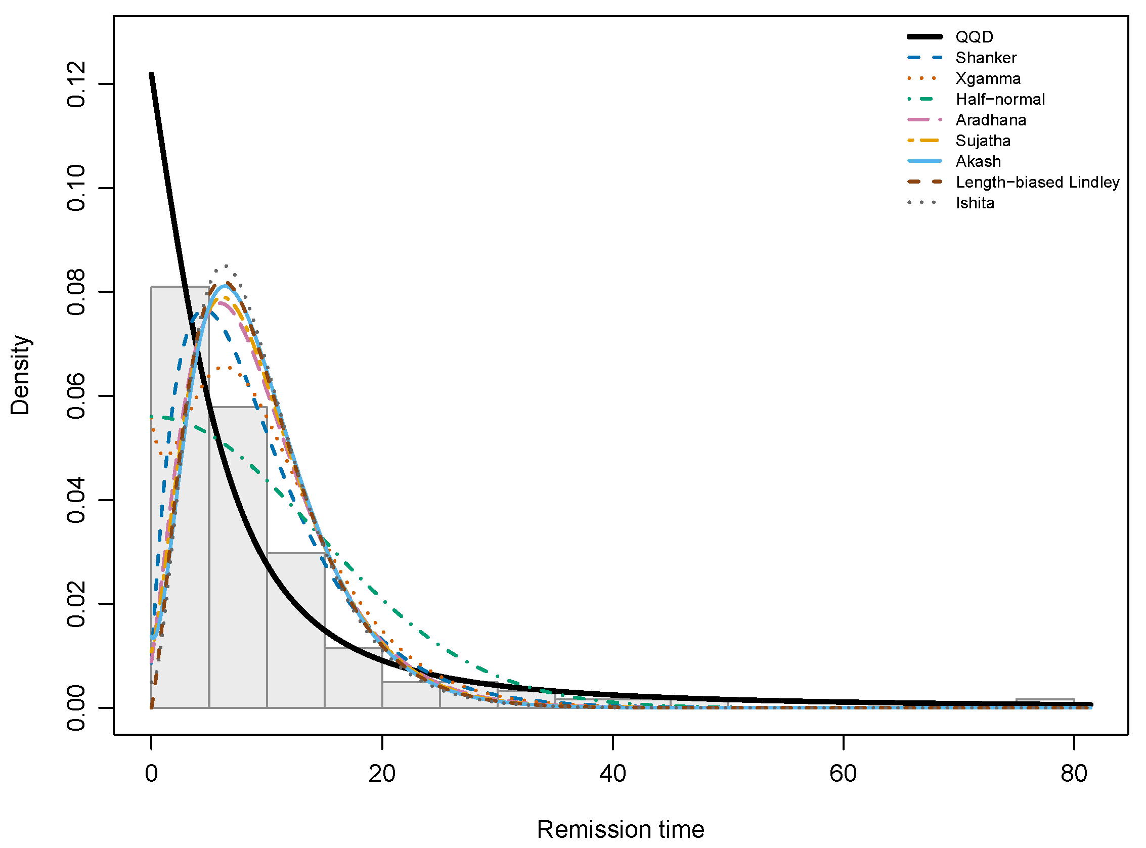
The third application considers the bladder-cancer remission-time data, consisting of $n=121$ positive observations. The sample exhibits marked positive skewness and substantial upper-tail variability, with most remission times concentrated in the lower and intermediate part of the support and a relatively small number of considerably larger observations. These characteristics provide a useful setting for examining the ability of the QQD to describe right-skewed biomedical duration data.

As in the preceding application, we consider a focused comparison among one-parameter lifetime distributions. In addition to the proposed QQD, the displayed competitors include the Shanker, Xgamma, Half-normal, Aradhana, Sujatha, Akash, Length-biased Lindley, Ishita, Amarendra, Rama, Pranav, Rayleigh, and Maxwell distributions. These models were selected from the broader numerical screening because the QQD attains smaller information-criterion values than each of them. Accordingly,

Table 4. Likelihood-based comparison of the QQD with selected one-parameter distributions for the bladder-cancer remission-time data ($n=121$). The best likelihood/information-criterion values are shown in bold.

Model	$\widehat{\mathit{\theta }}$	LogL	AIC	AICc	BIC	HQIC	CAIC
QQD	$\mathbf{4}.\mathbf{103}$	$-\mathbf{402}.\mathbf{036}$	$\mathbf{806}.\mathbf{072}$	$\mathbf{806}.\mathbf{105}$	$\mathbf{808}.\mathbf{867}$	$\mathbf{807}.\mathbf{207}$	$\mathbf{809}.\mathbf{867}$
Shanker	0.208	$-402.263$	806.526	806.559	809.321	807.661	810.321
Xgamma	0.266	$-407.130$	816.259	816.293	819.055	817.395	820.055
Half-normal	14.244	$-409.239$	820.479	820.512	823.275	821.614	824.275
Aradhana	0.287	$-415.006$	832.012	832.045	834.807	833.147	835.807
Sujatha	0.295	$-417.328$	836.655	836.689	839.451	837.791	840.451
Akash	0.306	$-420.982$	843.963	843.997	846.759	845.099	847.759
Length-biased Lindley	0.302	$-425.798$	853.595	853.629	856.391	854.730	857.391
Ishita	0.317	$-427.626$	857.252	857.285	860.048	858.387	861.048
Amarendra	0.401	$-446.018$	894.036	894.070	896.832	895.172	897.832
Rama	0.417	$-454.331$	910.662	910.696	913.458	911.798	914.458
Pranav	0.425	$-460.394$	922.789	922.822	925.585	923.924	926.585
Rayleigh	10.072	$-466.250$	934.501	934.534	937.297	935.636	938.297
Maxwell	8.224	$-546.246$	1094.493	1094.526	1097.289	1095.628	1098.289

should be interpreted as a selected benchmark comparison rather than as a complete ranking of every model examined computationally.

All models contain exactly one unknown parameter and are estimated by maximum likelihood. Consequently, differences among AIC, AICc, BIC, HQIC, and CAIC are driven entirely by differences in the maximized log-likelihood.

Within the selected comparison reported in Table 4, the QQD provides the most favorable likelihood-based fit. Its maximum likelihood estimate is

$$\widehat{\theta }=4.103,$$

and the maximized log-likelihood is $\log L=-402.036$. The model also attains the smallest values of all five information criteria,

$$\mathrm{AIC}=806.072,\mathrm{AICc}=806.105,\mathrm{BIC}=808.867,$$

$$\mathrm{HQIC}=807.207,\mathrm{CAIC}=809.867.$$

The Shanker distribution is the closest displayed competitor. Its maximized log-likelihood is $-402.263$, with AIC $=806.526$ and BIC $=809.321$. Hence,

$$\mathsf{\Delta }\mathrm{AIC}=806.526-806.072=0.454,$$

and

$$\mathsf{\Delta }\mathrm{BIC}=809.321-808.867=0.454.$$

Because both models contain exactly one unknown parameter, the same difference is retained, apart from rounding, for AICc, HQIC, and CAIC. The numerical separation between the QQD and Shanker distributions is therefore small, indicating that both models provide very similar likelihood-based representations of these remission-time data.

The distinction becomes clearer for the remaining competitors. The Xgamma distribution gives AIC $=816.259$, which is approximately $10.187$ units larger than the QQD value, while the Half-normal model has AIC $=820.479$, yielding a difference of approximately $14.407$. The Aradhana and Sujatha distributions produce AIC values of $832.012$ and $836.655$, respectively.

Still larger information-criterion values are obtained for the Akash, Length-biased Lindley, and Ishita distributions. Their AIC values are $843.963$, $853.595$, and $857.252$, respectively. The separation is particularly pronounced for the Amarendra, Rama, Pranav, Rayleigh, and Maxwell models, whose AIC values range from $894.036$ to $1094.493$.

Since all distributions displayed in Table 4 have the same number of unknown parameters, the favorable position of the QQD is not produced by a smaller model-complexity penalty. Rather, it follows directly from its larger maximized likelihood relative to the selected competitors.

From a distributional perspective, the result is consistent with the characteristics of the remission-time data. The QQD places substantial probability near the lower part of the support while retaining a slowly decaying upper tail. This combination is potentially useful for samples such as the present one, in which relatively short and moderate remission times coexist with a small number of considerably larger observations.

Overall, the bladder-cancer application provides evidence that the QQD can offer a competitive and parsimonious representation of strongly right-skewed biomedical duration data. The very small information-criterion difference between the QQD and Shanker distributions, however, suggests that their relative performance should not be judged from numerical criteria alone. Fitted cumulative-distribution and survival-function plots are therefore useful complements for assessing their agreement with the data, particularly in the upper tail.

The conclusions of this application are deliberately restricted to the models displayed in Table 4; they should not be interpreted as evidence that the QQD dominates every distribution considered in the broader numerical screening.

5.4. Overall Empirical Assessment

The three applications show that the QQD can provide a useful and parsimonious description of strongly right-skewed positive data. For the Kevlar 373/Epoxy sample, the model achieves a favorable balance between likelihood fit and simplicity. In the aircraft application, it performs well relative to the selected one-parameter competitors, while for the bladder-cancer data, its fit is very close to that of the Shanker distribution.

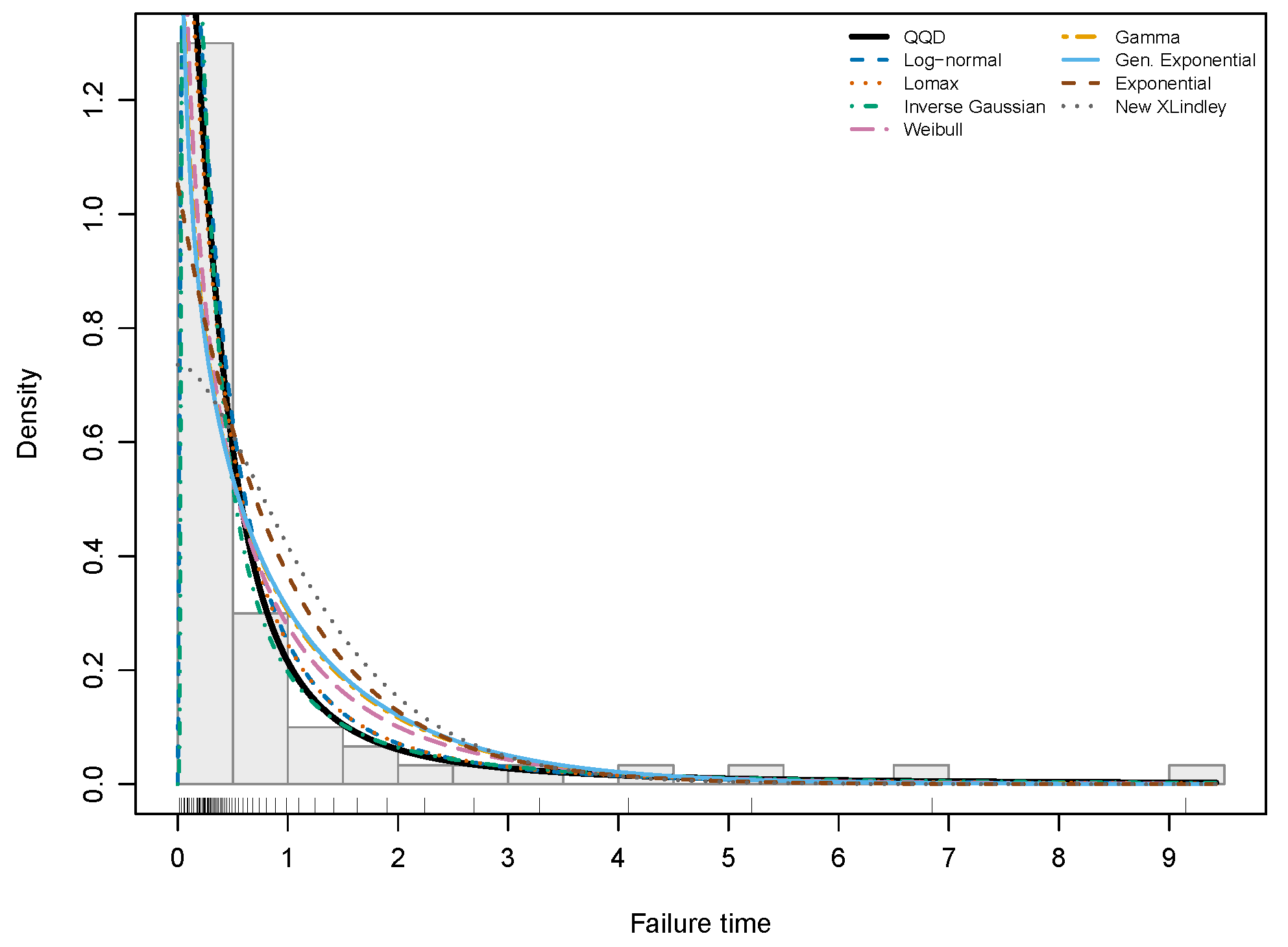
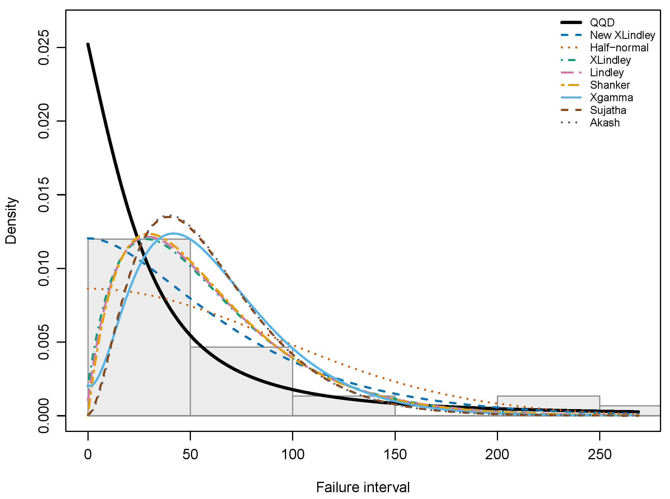
The graphical comparisons in Figure 7, Figure 8 and Figure 9 complement the information criteria by showing how the fitted models represent different parts of the data. This is especially important for the upper tail, since the QQD satisfies

$$\overline{F}\left(x\right)\sim {\displaystyle \frac{\theta }{x}},x\to \infty ,$$

and therefore has a slowly decaying Pareto-type tail.

This heavy-tail behavior is both a strength and a modeling limitation. It allows the QQD to accommodate unusually large observations, but it also implies an infinite ordinary mean. For this reason, the model is most naturally interpreted through quantiles, survival probabilities, and exceedance probabilities rather than mean-based summaries.

Overall, the empirical results support the QQD as a competitive one-parameter alternative for selected skewed datasets, without suggesting universal dominance. Its suitability should be assessed case by case using likelihood-based criteria together with graphical diagnostics, particularly in the upper tail.

6. Conclusions

This paper developed a quantile-based framework for constructing continuous probability distributions through differential equations satisfied directly by their quantile functions. In contrast with generator-based approaches that begin from a density or distribution function, the proposed quantile differential family (QDF) takes the quantile function as the primary modeling object. Under appropriate regularity conditions, the framework provides conditions ensuring the existence, uniqueness, and monotonicity of the resulting quantile function and, hence, the validity of the induced probability distribution.

As a concrete illustration, we introduced the one-parameter quadratic quantile distribution (QQD), whose quantile function is available in the explicit form

$$Q(u;\theta )=\theta {\displaystyle \frac{u(2-u)}{1-u}},0<u<1,\theta >0.$$

This simple representation leads to closed-form expressions for the distribution, density, survival, hazard, and cumulative hazard functions. Several additional properties were obtained, including quantile-based measures, entropy, stochastic ordering, and a detailed description of the upper-tail behavior.

A distinctive feature of the QQD is its regularly varying survival function,

$$\overline{F}\left(x\right)\sim {\displaystyle \frac{\theta }{x}},x\to \infty ,$$

which gives the model a Pareto-type tail with index one. This property allows the QQD to accommodate substantial upper-tail variability, but it also implies that the ordinary mean is infinite. The model should therefore be used in settings where such heavy-tailed behavior is scientifically plausible, with interpretation based primarily on quantiles, survival probabilities, exceedance probabilities, and other tail-oriented summaries.

Maximum likelihood estimation was developed for the QQD, and its finite-sample behavior was examined through Monte Carlo experiments. The simulations show that the estimator becomes increasingly accurate and less variable as the sample size grows over the scenarios considered. These numerical findings provide evidence of favorable finite-sample performance, but they are not intended to replace a formal proof of consistency or other asymptotic properties.

The empirical usefulness of the model was examined using three right-skewed datasets from reliability and biomedical applications. The QQD provided a competitive likelihood-based fit in the comparisons reported, while retaining only one unknown parameter. The real-data results also showed that relative performance depends on the dataset and on the competing models considered. Accordingly, the numerical results should not be interpreted as evidence of universal superiority. Likelihood-based criteria are most informative when considered together with graphical diagnostics, particularly in the upper tail where the QQD differs structurally from many light-tailed lifetime models.

More broadly, the QQD serves as one example of what can be obtained from the QDF construction. Other choices of the quantile differential generator may lead to models with different tail behavior, hazard shapes, and levels of flexibility. Possible extensions include multi-parameter and regression versions, inference under censoring or truncation, Bayesian estimation, and multivariate or dependent quantile-based constructions. These directions may help clarify the scope of the proposed framework and its usefulness in reliability, survival analysis, actuarial modeling, finance, and other areas where quantile-based descriptions are especially relevant.