Dynamic Behaviors of a Stage-Structured Commensalism Model with Holling Type II Benefits and Birth-Related Allee Effect

Abstract

Low adult density can suppress recruitment through mate limitation or cooperative reproductive failure, even when a host improves adult survival. Motivated by this ecological tension, we introduce a fecundity-related component Allee effect into a stage-structured commensalism model with a Holling type II host benefit. The nonlinear recruitment term is $f\left(x_2\right)=\alpha x_2^2/(x_2+A)$, and the independently growing host converges to its carrying capacity, yielding an asymptotically autonomous commensal subsystem. We obtain a complete analytical classification. If the long-term host benefit D exceeds mature mortality ${\delta }_2$, a unique coexistence equilibrium attracts every nontrivial commensal population. If the benefit is insufficient, fecundity limitation can instead create two positive equilibria: a low-density saddle whose stable set is the basin boundary and a stable high-density coexistence state. Thus, extinction and coexistence are both possible, depending on initial stage composition and host abundance. Stronger fecundity limitation enlarges the extinction region, whereas greater recruitment, maturation or host benefit promotes persistence. At the critical boundary, the positive equilibria merge in a non-degenerate saddle-node bifurcation. Rigorous global arguments and numerical comparisons with the linear-recruitment model show how a component Allee effect can induce strong-Allee-type demographic behavior, including bistability and threshold-mediated extinction.

1. Introduction

Commensalism is an ecological interaction in which one species benefits while the other is not directly affected. Classical examples include epiphytic plants growing on host trees, remoras attached to sharks, and inquiline organisms living in the nests or burrows of other species. Although commensalism has been modeled less often than competition, predation or mutualism, it is an important component of ecological networks and can substantially influence persistence, community assembly and biodiversity patterns. General discussions of symbiosis and commensalism go back to the classical ecological literature [1,2,3], and deterministic models for commensal symbiosis now range over Lotka–Volterra type systems, Holling-type benefit models, Michaelis–Menten response models, harvesting models, discrete-time systems and stage-structured systems.

Allee-type mechanisms have entered commensal symbiosis models from several directions. Chen [4] studied a two-species commensal model with an Allee effect in which one species cannot survive independently. Wu, Li and Lin [5] considered a Holling-type commensal symbiosis model involving the Allee effect, and Lin [6] showed that, under suitable conditions, the Allee effect may increase the final density of the affected species in a Lotka–Volterra commensal system. Lei [7] analyzed a Holling-type commensal system in which the first species is subject to an Allee effect. Commensalism models with additive or multiplicative Allee effects, discrete dynamics, spatial dispersal and harvesting are discussed in [8,9,10,11] and the references therein.

Harvesting and functional-response mechanisms have also been incorporated into commensalism models. Chen [12] analyzed a Lotka–Volterra commensal system with Michaelis–Menten-type harvesting, and boundary equilibria, persistence and stability for commensal or mixed symbiotic systems with harvesting were subsequently treated in [13,14,15,16,17]. Su et al. [18] studied a discrete commensalism model with non-selective harvesting, and further contributions have dealt with discrete systems, multi-species commensalism–amensalism models, delayed or stochastic commensal systems and bifurcation phenomena [19,20,21,22,23,24]. Among these, Chen, Li and Chen [25] investigated a stage-structured commensalism system with Holling Type II commensalistic benefits, which provides the starting point for the present work. Even though one species is not directly affected by the interaction, commensalistic systems can exhibit persistence, extinction, stability switches and bifurcations.

Stage structure is another fundamental feature of population dynamics. Individuals in different life stages differ in survival, reproduction, maturation and ecological roles, and stage-structured models, beginning with Aiello and Freedman [26], have been widely used in single-species dynamics, predator–prey interactions and symbiotic systems. In a stage-structured commensal population, only mature individuals reproduce, and immature individuals mature at a certain rate; low mature density can therefore severely suppress population growth even when immature individuals are abundant. This mechanism makes stage-structured populations particularly susceptible to Allee-type phenomena.

The Allee effect, first discussed by Allee and later formalized in population ecology, refers to a positive relationship between individual fitness and population density at low densities [27,28,29,30,31]. Its mechanisms include mate-finding limitation, cooperative breeding failure, predator dilution, social facilitation and genetic constraints. Allee effects may be weak or strong: a weak Allee effect reduces the per-capita growth rate at low densities without making it negative at zero density, whereas a strong Allee effect introduces a critical threshold below which the population declines to extinction [32,33,34,35,36]. Allee effects have been incorporated into single-species models, age- and stage-structured models, predator–prey systems, epidemic-ecological models and spatial dispersal models [37,38,39,40,41,42]. Birth-related or fecundity-related Allee effects are biologically natural when reproduction is limited by mature population density, mating success or cooperative reproduction.

Empirical mechanisms motivating such a recruitment law include pollen limitation in sparse animal-pollinated plants, gamete dilution in broadcast spawning marine invertebrates, failure to locate mates in rare or invading populations, and reduced breeding success in cooperatively reproducing vertebrates. In a stage-structured population, these mechanisms act primarily through mature individuals, while juveniles contribute only after maturation. The examples motivate the functional form qualitatively; the present study is a theoretical investigation and is not calibrated to a particular taxon.

Chen, Li and Chen [25] proposed the stage-structured commensalism model

$$\left\{\begin{array}{c}{\displaystyle \frac{d{x}_1}{dt}}=\alpha x_2-(\beta +{\delta }_1)x_1,\hfill \\ {\displaystyle \frac{d{x}_2}{dt}}=\beta x_1-{\delta }_2{x}_2-\gamma x_2^2+d·{\displaystyle \frac{y}{{\eta }_1+{\eta }_{2}y}}·x_2,\hfill \\ {\displaystyle \frac{dy}{dt}}=y(b_2-a_{2}y),\hfill \end{array}\right.$$

(1)

in which $x_1$ and $x_2$ are the immature and mature densities of the commensal species and y is the host density; all parameters are positive. In (1), the birth rate of immature commensals is linear in the mature density. If mature individuals are scarce, however, mate-finding difficulties or cooperative reproductive failure reduce the per-capita birth rate. To capture this effect, we replace the linear birth term by the saturating weak-Allee birth function

$$\alpha x_2⟼{\displaystyle \frac{\alpha x_2^2}{x_2+A}},A>0.$$

(2)

This function satisfies $f\left(0\right)=0$, $f\left(x\right)>0$ for $x>0$, $f\left(x\right)<\alpha x$ for $x>0$, and $f\left(x\right)/x\to 0$ as $x\to 0^{+}$, which is consistent with a weak birth-related Allee effect.

Our aim is to determine how this modification changes the global dynamics of (1). The sign of $D-{\delta }_2$, where D denotes the commensal benefit at the host equilibrium, divides the parameter space into two regimes. If $D>{\delta }_2$, the commensal benefit is strong enough to guarantee global coexistence; if $D<{\delta }_2$, the Allee effect creates a threshold phenomenon, and, depending on reproductive capacity and the intensity of the Allee effect, the system is either bistable between extinction and coexistence or loses all positive equilibria through a saddle-node bifurcation. When $A=0$, system (3) reduces to the stage-structured commensalism model studied in [25], which admits neither bistability nor threshold-driven extinction; the birth-related Allee effect is thus the sole mechanism responsible for the bistable and saddle-node structures obtained below. We distinguish carefully between a component Allee effect in fecundity and a strong Allee effect in net population growth. Here, recruitment is nonnegative but its per-capita value tends to zero at low mature density. When host benefit does not compensate mature mortality, that component mechanism produces strong-Allee-type demographic behavior: an unstable low-density coexistence state and a basin boundary between extinction and persistence (Remark 1). Our contribution is therefore not a new host–commensal architecture, nor a claim that bistability itself is new; it is an analytical characterization of how this particular fecundity mechanism changes the established stage-structured model (Table 1).

Table 1. Comparison with the linear-recruitment model of Chen, Li and Chen [25].

Feature	Earlier Model ($\mathit{A}=0$)	Present Model ($\mathit{A}>0$)
Recruitment	$\alpha x_2$	$\alpha x_2^2/(x_2+A)$
Per-capita recruitment near zero	approaches α	approaches zero
Positive equilibria	no Allee-generated pair	zero, one double or two
Low-density basin boundary	absent from this mechanism	stable set of a low-density saddle
New qualitative consequence	no fecundity-induced saddle-node	bistability, threshold-mediated extinction and saddle-node bifurcation

The remainder of this paper is organized as follows. Section 2 formulates the model, records the basic invariance and boundedness facts, and derives all equilibria. Section 3 gives the local stability criteria. Section 4 treats the strong-benefit case $D>{\delta }_2$ and proves global stability of the unique positive equilibrium. Section 5 analyzes the weak-benefit case $D<{\delta }_2$, including the existence threshold, bistability, threshold-driven extinction and the associated Allee threshold. Section 6 discusses the boundary case $D={\delta }_2$ and the saddle-node bifurcation, and presents a parameter-regime diagram. Section 7 reports numerical experiments, and Section 8 concludes.

2. The Model and Preliminaries

We study the stage-structured commensalism model

$$\left\{\begin{array}{c}{\displaystyle \frac{d{x}_1}{dt}}={\displaystyle \frac{\alpha x_2^2}{x_2+A}}-(\beta +{\delta }_1)x_1,\hfill \\ {\displaystyle \frac{d{x}_2}{dt}}=\beta x_1-{\delta }_2{x}_2-\gamma x_2^2+d·{\displaystyle \frac{y}{{\eta }_1+{\eta }_{2}y}}·x_2,\hfill \\ {\displaystyle \frac{dy}{dt}}=y(b_2-a_{2}y),\hfill \end{array}\right.$$

(3)

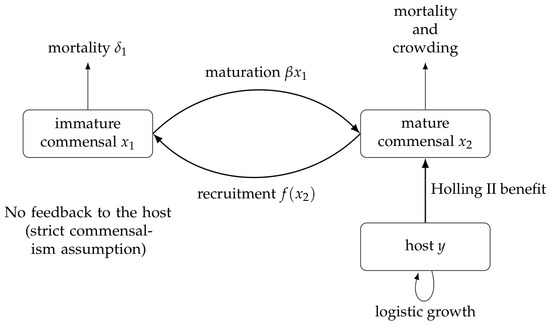
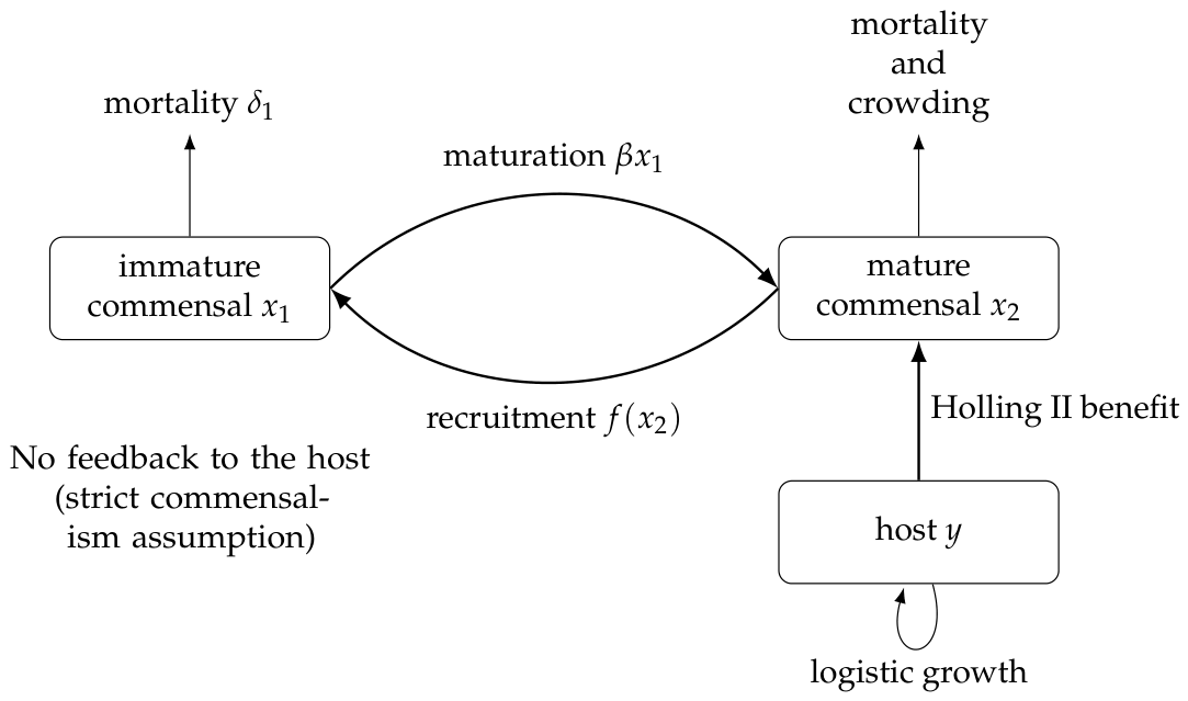
where $x_1\left(t\right)$, $x_2\left(t\right)$ and $y\left(t\right)$ denote the immature commensal, mature commensal and host populations, respectively, and all parameters are positive. The term $\alpha x_2^2/(x_2+A)$ is the saturating recruitment function (2), and the host equation is logistic. The commensal benefit $d·y/({\eta }_1+{\eta }_{2}y)·x_2$ acts on the mature class, reducing the effective mature mortality; a schematic of the model is shown in Figure 1.

Figure 1. Schematic of the stage transitions and one-way commensalistic interaction. The absence of feedback from the commensal to the host renders the system triangular.

We assume nonnegative initial densities and positive parameter values. The model can be interpreted in dimensional units satisfying the consistency shown in Table 2, or after scaling density and time. Because the simulations are intended to test qualitative regimes rather than fit a particular species, all numerical parameter values below are illustrative.

Table 2. State variables and parameters. Density and time units may be chosen for a target system; the numerical section uses scaled, illustrative units.

Symbol	Biological Meaning	Dimension
$x_1,x_2,y$	immature commensal, mature commensal and host densities	density
α	maximal per-capita recruitment coefficient	time−1
β	maturation rate	time−1
${\delta }_1,{\delta }_2$	immature and mature mortality rates	time−1
γ	mature density-dependence coefficient	1/(density·time)
A	mature-density scale of fecundity limitation	density
d	strength of the host-provided mature benefit	scaled rate
${\eta }_1,{\eta }_2$	half-saturation scaling constants	scaled units
b2	intrinsic host growth rate	time−1
a2	host density-dependence coefficient	1/(density·time)

We introduce the auxiliary quantities

$$f\left(x\right)={\displaystyle \frac{\alpha x^2}{x+A}},D\left(y\right)={\displaystyle \frac{dy}{{\eta }_1+{\eta }_{2}y}},y^{*}={\displaystyle \frac{b_2}{a_2}},D=D\left(y^{*}\right)={\displaystyle \frac{d{b}_2/a_2}{{\eta }_1+{\eta }_2{b}_2/a_2}}.$$

(4)

Then $f\left(0\right)=0$, $f\left(x\right)>0$ for $x>0$, and

$$f^{\prime }\left(x\right)={\displaystyle \frac{\alpha x(x+2A)}{{(x+A)}^2}}>0,f\left(x\right)<\alpha x(x>0),\underset{x\to 0^{+}}{\lim }{\displaystyle \frac{f\left(x\right)}{x}}=0.$$

The last two relations identify a component Allee effect in fecundity: recruitment is depressed at low mature density and its per-capita value tends to zero. Because a birth flux cannot itself be negative, the conventional weak/strong distinction based on the sign of total per-capita population growth is deferred to the demographic outcome obtained for the full system below.

Since the host equation is logistic,

$$\underset{t\to +\infty }{\lim }y\left(t\right)=y^{*},y\left(0\right)>0,$$

(5)

so the full system (3) is asymptotically autonomous, with limiting flow obtained by setting $y=y^{*}$ in the first two equations.

Lemma 1. 

The nonnegative cone ${\mathbb{R}}_{+}^3=\{(x_1,x_2,y):x_1,x_2,y\ge 0\}$ is positively invariant for (3). Every solution with initial value in ${\mathbb{R}}_{+}^3$ exists globally and is bounded.

Proof. 

On the boundary of ${\mathbb{R}}_{+}^3$, $x_1=0$ implies ${\dot{x}}_1=f\left(x_2\right)\ge 0$, $x_2=0$ implies ${\dot{x}}_2=\beta x_1\ge 0$, and $y=0$ implies $\dot{y}=0$; hence ${\mathbb{R}}_{+}^3$ is positively invariant.

Because $y\left(t\right)$ solves a logistic equation, $0\le y\left(t\right)\le M_y:=\max \{y\left(0\right),y^{*}\}$, so $0\le D\left(y\left(t\right)\right)\le \overline{D}:=d{M}_y/({\eta }_1+{\eta }_2{M}_y)$. Let $E=x_1+x_2$. Using $f\left(x_2\right)\le \alpha x_2$ and $D\left(y\right)\le \overline{D}$,

$$\begin{array}{cc}\hfill \dot{E}& =f\left(x_2\right)-(\beta +{\delta }_1)x_1+\beta x_1+(D\left(y\right)-{\delta }_2)x_2-\gamma x_2^2\hfill \\ & =f\left(x_2\right)-{\delta }_1{x}_1+(D\left(y\right)-{\delta }_2)x_2-\gamma x_2^2\hfill \\ & \le \alpha x_2-{\delta }_1{x}_1+(\overline{D}-{\delta }_2)x_2-\gamma x_2^2\hfill \\ & =-{\delta }_{1}E+(\alpha +{\delta }_1+\overline{D}-{\delta }_2)x_2-\gamma x_2^2.\hfill \end{array}$$

The concave parabola in $x_2$ on the right-hand side is bounded above, so $\dot{E}\le -{\delta }_{1}E+K$ for some constant $K>0$, and hence $E\left(t\right)\le \max \{E\left(0\right),K/{\delta }_1\}$. Thus, $x_1\left(t\right)$ and $x_2\left(t\right)$ are bounded, and global existence follows from standard ODE theory.    □

The boundary equilibria of (3) are

$$E_0=(0,0,0),E_1=(0,0,y^{*}).$$

A commensal-only equilibrium $E_2=({\tilde{x}}_1,{\tilde{x}}_2,0)$ with ${\tilde{x}}_2>0$ would satisfy ${\tilde{x}}_1=f\left({\tilde{x}}_2\right)/(\beta +{\delta }_1)$ and

$$\gamma (\beta +{\delta }_1)x_2^2+\left[(\beta +{\delta }_1)({\delta }_2+\gamma A)-\alpha \beta \right]x_2+{\delta }_2(\beta +{\delta }_1)A=0.$$

(6)

The plane $y=0$ is invariant but unreachable from $y\left(0\right)>0$, so $E_2$ plays no role in the dynamics of the biologically meaningful region.

A positive equilibrium $E_3=(x_1^{**},x_2^{**},y^{*})$ satisfies $x_1^{**}=f\left(x_2^{**}\right)/(\beta +{\delta }_1)$ and

$${\displaystyle \frac{\beta f\left(x_2^{**}\right)}{\beta +{\delta }_1}}+(D-{\delta }_2)x_2^{**}-\gamma {\left(x_2^{**}\right)}^2=0.$$

Multiplying by $(\beta +{\delta }_1)(x_2^{**}+A)$ and discarding the root $x_2^{**}=0$, we find that $x_2^{**}$ is a positive root of

$$P{x}_2^2+Q_1{x}_2+R_1=0,$$

(7)

where

$$P=\gamma (\beta +{\delta }_1)>0,Q_1=(\beta +{\delta }_1)(\gamma A+{\delta }_2-D)-\alpha \beta ,R_1=-(D-{\delta }_2)(\beta +{\delta }_1)A.$$

The sign of $R_1$ separates two regimes. If $D>{\delta }_2$, then $R_1<0$, and (7) has exactly one positive root; this is the strong-benefit case treated in Section 4. If $D<{\delta }_2$, then $R_1>0$, and positive roots exist only under a further threshold condition; this is the weak-benefit case treated in Section 5.

At $D={\delta }_2$, Equation (7) reduces to $x_2(P{x}_2+Q_1)=0$ with $Q_1=(\beta +{\delta }_1)\gamma A-\alpha \beta$, so a positive equilibrium emerges from the boundary precisely when $\alpha \beta >(\beta +{\delta }_1)\gamma A$, that is, $X>Y$ in the notation introduced in Section 5.

3. Local Stability Analysis

The Jacobian of (3) is

$$J(x_1,x_2,y)=\left(\begin{array}{ccc}-(\beta +{\delta }_1)& f^{\prime }\left(x_2\right)& 0\\ \beta & D\left(y\right)-{\delta }_2-2\gamma x_2& {\displaystyle \frac{d{\eta }_1{x}_2}{{({\eta }_1+{\eta }_{2}y)}^2}}\\ 0& 0& b_2-2a_{2}y\end{array}\right),$$

(8)

with $f^{\prime }\left(x\right)=\alpha x(x+2A)/{(x+A)}^2$.

Proposition 1. 

The origin $E_0$ is unstable. The host-only equilibrium $E_1=(0,0,y^{*})$ is locally asymptotically stable when $D<{\delta }_2$ and unstable when $D>{\delta }_2$; at $D={\delta }_2$, it is non-hyperbolic.

Proof. 

At $E_0$, the eigenvalues of (8) are $-(\beta +{\delta }_1)$, $-{\delta }_2$, and $b_2$, so $E_0$ is a saddle. At $E_1$,

$$J\left(E_1\right)=\left(\begin{array}{ccc}-(\beta +{\delta }_1)& 0& 0\\ \beta & D-{\delta }_2& 0\\ 0& 0& -b_2\end{array}\right),$$

whose eigenvalues are $-(\beta +{\delta }_1)$, $D-{\delta }_2$, and $-b_2$. The conclusion follows.    □

At a positive equilibrium $E_3$, the host direction contributes the eigenvalue $-b_2<0$, so stability is decided by the planar block  

$$J_2=\left(\begin{array}{cc}-(\beta +{\delta }_1)& f^{\prime }\left(x_2^{**}\right)\\ \beta & D-{\delta }_2-2\gamma x_2^{**}\end{array}\right),$$

whose characteristic polynomial is ${\lambda }^2+C_1\lambda +C_2=0$ with

$$\begin{array}{cc}\hfill C_1& =(\beta +{\delta }_1)+2\gamma x_2^{**}+{\delta }_2-D,\hfill \end{array}$$

(9)

$$\begin{array}{cc}\hfill C_2& =(\beta +{\delta }_1)(2\gamma x_2^{**}+{\delta }_2-D)-\beta f^{\prime }\left(x_2^{**}\right).\hfill \end{array}$$

(10)

Using the equilibrium relation

$${\displaystyle \frac{\beta f\left(x_2^{**}\right)}{\beta +{\delta }_1}}=\gamma {\left(x_2^{**}\right)}^2+({\delta }_2-D)x_2^{**},$$

a short computation gives

$$C_2=x_2^{**}\left[(\beta +{\delta }_1)\gamma -{\displaystyle \frac{\beta \alpha A}{{(x_2^{**}+A)}^2}}\right].$$

(11)

Define

$$h\left(x\right)=(\beta +{\delta }_1)\gamma -{\displaystyle \frac{\beta \alpha A}{{(x+A)}^2}}.$$

(12)

Then, $C_2=x_2^{**}h\left(x_2^{**}\right)$. The function h is strictly increasing, and it has a positive zero exactly when $\alpha \beta >(\beta +{\delta }_1)\gamma A$; the zero is then

$$x_{\mathrm{crit}}=\sqrt{{\displaystyle \frac{\beta \alpha A}{(\beta +{\delta }_1)\gamma }}}-A.$$

(13)

Lemma 2. 

For a positive equilibrium $E_3$,

$$\mathrm{sgn}\left(C_2\right)=\left\{\begin{array}{cc}-1,\hfill & 0<x_2^{**}<x_{\mathrm{crit}},\hfill \\ 0,\hfill & x_2^{**}=x_{\mathrm{crit}},\hfill \\ +1,\hfill & x_2^{**}>x_{\mathrm{crit}},\hfill \end{array}\right.$$

whenever $x_{\mathrm{crit}}>0$; if $x_{\mathrm{crit}}\le 0$, then $C_2>0$ at every positive equilibrium.

Proof. 

Since h is strictly increasing and $C_2=x_2^{**}h\left(x_2^{**}\right)$, the claim is immediate.    □

4. Global Stability for $\mathit{D}>{\mathit{\delta }}_{\mathbf{2}}$

Throughout this section $D>{\delta }_2$, and we write ${\Delta }_1=D-{\delta }_2>0$; this is the negative of the quantity $\Delta ={\delta }_2-D$ used in Section 5. In the limit $y=y^{*}$, the system (3) reduces to the planar system

$$\left\{\begin{array}{c}{\dot{x}}_1=f\left(x_2\right)-(\beta +{\delta }_1)x_1,\hfill \\ {\dot{x}}_2=\beta x_1+{\Delta }_1{x}_2-\gamma x_2^2.\hfill \end{array}\right.$$

(14)

Lemma 3. 

If $D>{\delta }_2$, the unique positive equilibrium satisfies $x_2^{**}>\max \{0,x_{\mathrm{crit}}\}$, and hence $C_2>0$.

Proof. 

Since $P>0$ and $R_1=-(D-{\delta }_2)(\beta +{\delta }_1)A<0$, Equation (7) has exactly one positive root $x_2^{**}$. If $x_{\mathrm{crit}}\le 0$, then $C_2>0$ is clear from (11). Suppose $x_{\mathrm{crit}}>0$, and set

$$g\left(x\right)={\displaystyle \frac{\beta f\left(x\right)}{\beta +{\delta }_1}}+{\Delta }_{1}x-\gamma x^2.$$

The positive zeros of g are the positive roots of (7). Since $g\left(0\right)=0$, $g^{\prime }\left(0\right)={\Delta }_1>0$, and $g\left(x\right)\to -\infty$ as $x\to +\infty$, the unique positive zero $x_2^{**}$ satisfies $g>0$ on $(0,x_2^{**})$ and $g<0$ on $(x_2^{**},\infty )$. A direct computation gives

$$g\left(x_{\mathrm{crit}}\right)=x_{\mathrm{crit}}\left[{(X-Y)}^2+{\Delta }_1\right]>0,$$

where $X=\sqrt{\alpha \beta /(\beta +{\delta }_1)}$ and $Y=\sqrt{\gamma A}$. Hence, $x_2^{**}>x_{\mathrm{crit}}$, and $C_2=x_2^{**}h\left(x_2^{**}\right)>0$ by monotonicity of h.    □

Theorem 1. 

If $D>{\delta }_2$, the unique positive equilibrium $E_3$ is locally asymptotically stable.

Proof. 

By Lemma 3, $C_2>0$. From the equilibrium equation,

$$\gamma x_2^{**}={\displaystyle \frac{\beta f\left(x_2^{**}\right)}{(\beta +{\delta }_1)x_2^{**}}}+{\Delta }_1,$$

and therefore

$$C_1=(\beta +{\delta }_1)+2\gamma x_2^{**}-{\Delta }_1=(\beta +{\delta }_1)+{\displaystyle \frac{2\beta f\left(x_2^{**}\right)}{(\beta +{\delta }_1)x_2^{**}}}+{\Delta }_1>0.$$

The Routh–Hurwitz criterion yields local asymptotic stability.    □

Lemma 4. 

For every fixed value of D, the planar system

$${\dot{x}}_1=f\left(x_2\right)-(\beta +{\delta }_1)x_1,{\dot{x}}_2=\beta x_1+(D-{\delta }_2)x_2-\gamma x_2^2$$

has no periodic orbit in the open positive quadrant.

Proof. 

With $B(x_1,x_2)=1/x_2$,

$${\displaystyle \frac{\partial }{\partial x_1}}\left({\displaystyle \frac{{\dot{x}}_1}{x_2}}\right)+{\displaystyle \frac{\partial }{\partial x_2}}\left({\displaystyle \frac{{\dot{x}}_2}{x_2}}\right)=-{\displaystyle \frac{\beta +{\delta }_1}{x_2}}-{\displaystyle \frac{\beta x_1}{x_2^2}}-\gamma <0$$

for $x_1,x_2>0$. By the Bendixson–Dulac criterion, no closed orbit lies in the positive quadrant.    □

Corollary 1. 

For every fixed value of D, the planar system

$${\dot{x}}_1=f\left(x_2\right)-(\beta +{\delta }_1)x_1,{\dot{x}}_2=\beta x_1+(D-{\delta }_2)x_2-\gamma x_2^2$$

has no periodic orbit, homoclinic loop, or heteroclinic cycle in the closed positive quadrant. Every bounded positive orbit has an omega-limit set that contains an equilibrium; in each parameter regime considered below, it converges to one equilibrium.

Proof. 

The axes, except for the origin, are not invariant: at $x_1=0,x_2>0$, ${\dot{x}}_1=f\left(x_2\right)>0$, while at $x_2=0,x_1>0$, ${\dot{x}}_2=\beta x_1>0$. Thus, a closed invariant curve cannot use a boundary segment and would have to lie in the open quadrant. On every compact subregion, there the multiplier $B=1/x_2$ is $C^1$, and the strictly negative divergence in Lemma 4, together with Green’s theorem, excludes periodic orbits and closed separatrix polygons (including homoclinic and heteroclinic cycles). The Poincaré–Bendixson theorem then implies that a compact omega-limit set without an equilibrium would be periodic, which is impossible. Finally, in the regimes below, there are finitely many hyperbolic equilibria (apart from the separately treated saddle-node value); the absence of separatrix cycles prevents an omega-limit set from being a polycycle. Connectedness and invariance therefore force convergence to one equilibrium.    □

Theorem 2. 

Assume $D>{\delta }_2$. Then, the unique positive equilibrium $E_3=(x_1^{**},x_2^{**},y^{*})$ is globally asymptotically stable for all initial values satisfying

$$x_1\left(0\right)\ge 0,x_2\left(0\right)\ge 0,x_1\left(0\right)+x_2\left(0\right)>0,y\left(0\right)>0.$$

Proof. 

By Lemma 1, all solutions are bounded, and $y\left(t\right)\to y^{*}$ exponentially.

Consider first the limiting planar system (14). Its origin is a hyperbolic saddle with eigenvalues $-(\beta +{\delta }_1)<0$ and ${\Delta }_1>0$. No orbit in the open positive quadrant can converge to the origin: if $x_2\left(t\right)\to 0$ along such an orbit, then $0<x_2\left(t\right)<{\Delta }_1/\gamma$ for all sufficiently large t, and since $x_1\left(t\right)\ge 0$,

$${\dot{x}}_2\left(t\right)=\beta x_1\left(t\right)+{\Delta }_1{x}_2\left(t\right)-\gamma x_2{\left(t\right)}^2\ge {\Delta }_1{x}_2\left(t\right)-\gamma x_2{\left(t\right)}^2>0,$$

contradicting $x_2\left(t\right)\to 0$. By Corollary 1, the limiting planar flow has no periodic orbit, homoclinic orbit or heteroclinic cycle in the closed positive quadrant, and the only equilibria of (14) there are the origin and $E_3$. The Poincaré–Bendixson theorem therefore forces every interior orbit to converge to $E_3$. If $x_2\left(0\right)=0$ and $x_1\left(0\right)>0$, then ${\dot{x}}_2\left(0\right)=\beta x_1\left(0\right)>0$, and the orbit enters the positive quadrant, so the same conclusion holds.

It remains to exclude convergence to $E_1=(0,0,y^{*})$ for the full system. Since $D\left(y\left(t\right)\right)\to D>{\delta }_2$, choose T such that

$$D\left(y\left(t\right)\right)-{\delta }_2\ge \frac{1}{2}(D-{\delta }_2)>0(t\ge T).$$

If $(x_1\left(t\right),x_2\left(t\right))\to (0,0)$ along a solution with $x_2\left(t\right)>0$, then $x_2\left(t\right)<(D-{\delta }_2)/\left(2\gamma \right)$ eventually, and

$${\dot{x}}_2\left(t\right)=\beta x_1\left(t\right)+(D\left(y\left(t\right)\right)-{\delta }_2)x_2\left(t\right)-\gamma x_2{\left(t\right)}^2\ge {\displaystyle \frac{D-{\delta }_2}{2}}{x}_2\left(t\right)-\gamma x_2{\left(t\right)}^2>0,$$

contradicting $x_2\left(t\right)\to 0$. Hence, $E_1$ is not an omega-limit point.

The full system is asymptotically autonomous with limiting flow (14). The convergence theorem for precompact asymptotically autonomous semiflows [43,44] makes its omega-limit set a nonempty compact connected internally chain transitive invariant set of the limit flow. Corollary 1 and the Poincaré–Bendixson classification leave only equilibria or a separatrix cycle; the latter has already been excluded by the Dulac argument, including on the boundary. Consequently, the omega-limit set is one equilibrium. Its only candidates are the origin and $E_3$, and the preceding differential inequality excludes the origin for every nontrivial commensal initial condition. Hence, the omega-limit set is $\left\{E_3\right\}$. Lyapunov stability follows from local asymptotic stability (Theorem 1), completing the global argument.    □

5. Dynamics for $\mathit{D}<{\mathit{\delta }}_{\mathbf{2}}$

Set

$$\Delta ={\delta }_2-D>0,$$

(15)

which is the negative of the parameter ${\Delta }_1$ of Section 4. Then, (7) becomes

$$P{x}_2^2+Q_1{x}_2+R_1=0,$$

(16)

with

$$P=\gamma (\beta +{\delta }_1),Q_1=(\beta +{\delta }_1)(\gamma A+\Delta )-\alpha \beta ,R_1=\Delta (\beta +{\delta }_1)A>0.$$

We introduce

$$X=\sqrt{{\displaystyle \frac{\alpha \beta }{\beta +{\delta }_1}}},Y=\sqrt{\gamma A}.$$

(17)

These composite quantities have direct threshold interpretations. $X^2$ measures effective recruitment into the mature population after the competition between maturation and immature mortality; $Y^2=\gamma A$ combines the density scale of fecundity limitation with mature crowding; $\Delta ={\delta }_2-D$ is the mature-mortality deficit remaining after the long-term host benefit; and D is that benefit evaluated at host carrying capacity. As shown below, persistence requires $X>Y+\sqrt{\Delta }$: the effective reproductive capacity must exceed both the fecundity–crowding barrier and the residual mortality barrier. It also predicts biologically that increasing $\alpha$, $\beta$ or d promotes persistence, whereas increasing A, ${\delta }_1$, ${\delta }_2$ or $\gamma$ makes persistence more difficult (with other parameters fixed).

Lemma 5. 

For $D<{\delta }_2$,

$$Q_1^2-4P{R}_1={(\beta +{\delta }_1)}^2\left[{(X^2-Y^2-\Delta )}^2-4Y^2\Delta \right].$$

Proof. 

A direct calculation gives

$$\begin{array}{cc}\hfill Q_1^2-4P{R}_1& ={\left[(\beta +{\delta }_1)(\gamma A+\Delta )-\alpha \beta \right]}^2-4\gamma (\beta +{\delta }_1)\Delta (\beta +{\delta }_1)A\hfill \\ & ={(\beta +{\delta }_1)}^2\left[{(Y^2+\Delta -X^2)}^2-4Y^2\Delta \right]\hfill \\ & ={(\beta +{\delta }_1)}^2\left[{(X^2-Y^2-\Delta )}^2-4Y^2\Delta \right].\hfill \end{array}$$

   □

Because $P>0$ and $R_1>0$, positive roots of (16) require $Q_1<0$, that is, $X^2>Y^2+\Delta$. Under this condition, the discriminant condition $Q_1^2-4P{R}_1\ge 0$ reads $X^2-Y^2-\Delta \ge 2Y\sqrt{\Delta }$, or equivalently

$$X\ge Y+\sqrt{\Delta }.$$

(18)

Theorem 3. 

Assume $D<{\delta }_2$, and let $\Delta ={\delta }_2-D>0$. If $X>Y+\sqrt{\Delta }$, system (3) has two distinct positive equilibria

$$E_3^{\mathrm{low}}=(x_{1,\mathrm{small}}^{**},x_{2,\mathrm{small}}^{**},y^{*}),E_3^{\mathrm{high}}=(x_{1,\mathrm{large}}^{**},x_{2,\mathrm{large}}^{**},y^{*}),$$

with $0<x_{2,\mathrm{small}}^{**}<x_{2,\mathrm{large}}^{**}$ and $x_{1,i}^{**}=f\left(x_{2,i}^{**}\right)/(\beta +{\delta }_1)$. If $X=Y+\sqrt{\Delta }$, there is exactly one positive equilibrium of multiplicity two; if $X<Y+\sqrt{\Delta }$, there is none.

Proof. 

The positive roots of (16), when they exist, are

$$x_{2,\mathrm{small}}^{**}={\displaystyle \frac{-Q_1-\sqrt{Q_1^2-4P{R}_1}}{2P}},x_{2,\mathrm{large}}^{**}={\displaystyle \frac{-Q_1+\sqrt{Q_1^2-4P{R}_1}}{2P}}.$$

Since $P>0$ and $R_1>0$, both roots are positive precisely when $Q_1<0$ and the discriminant is nonnegative; by Lemma 5 and the discussion preceding it, these conditions are equivalent to $X\ge Y+\sqrt{\Delta }$. Strict inequality gives two distinct roots, equality gives a double root, and the reverse inequality gives none.    □

Lemma 6. 

Assume $D<{\delta }_2$ and $X>Y+\sqrt{\Delta }$. Then,

$$0<x_{2,\mathrm{small}}^{**}<x_{\mathrm{crit}}<x_{2,\mathrm{large}}^{**}.$$

Proof. 

Let $g\left(x\right)=\beta f\left(x\right)/(\beta +{\delta }_1)-\Delta x-\gamma x^2$. The positive zeros of g are precisely $x_{2,\mathrm{small}}^{**}$ and $x_{2,\mathrm{large}}^{**}$. Since $g\left(0\right)=0$ and $g^{\prime }\left(0\right)=-\Delta <0$, g is negative just to the right of 0. A direct computation gives

$$g\left(x_{\mathrm{crit}}\right)=x_{\mathrm{crit}}\left[{(X-Y)}^2-\Delta \right]>0,$$

because $X>Y+\sqrt{\Delta }$ implies ${(X-Y)}^2>\Delta$. As $g\left(x\right)\to -\infty$ when $x\to +\infty$, the first positive zero lies in $(0,x_{\mathrm{crit}})$ and the second in $(x_{\mathrm{crit}},\infty )$.    □

Theorem 4. 

Assume $D<{\delta }_2$ and $X>Y+\sqrt{\Delta }$. Then, $E_1$ is locally asymptotically stable, $E_3^{\mathrm{low}}$ is a saddle, and $E_3^{\mathrm{high}}$ is locally asymptotically stable.

Proof. 

The stability of $E_1$ follows from Proposition 1. By Lemma 6, $x_{2,\mathrm{small}}^{**}<x_{\mathrm{crit}}$, so $C_2<0$ by Lemma 2; the planar block then has one positive and one negative eigenvalue, and together with the host eigenvalue $-b_2<0$, this makes $E_3^{\mathrm{low}}$ a saddle. For $E_3^{\mathrm{high}}$, $x_{2,\mathrm{large}}^{**}>x_{\mathrm{crit}}$, so $C_2>0$, and

$$C_1=(\beta +{\delta }_1)+2\gamma x_{2,\mathrm{large}}^{**}+\Delta >0,$$

so both planar eigenvalues have negative real parts; with the host eigenvalue, $E_3^{\mathrm{high}}$ is locally asymptotically stable.    □

Theorem 5. 

Assume $D<{\delta }_2$ and $X<Y+\sqrt{\Delta }$. Then, no positive equilibrium exists, and the host-only equilibrium $E_1=(0,0,y^{*})$ attracts every solution with $x_1\left(0\right)\ge 0$, $x_2\left(0\right)\ge 0$, $x_1\left(0\right)+x_2\left(0\right)>0$, and $y\left(0\right)>0$.

Proof. 

By Theorem 3, the limiting planar system has no positive equilibrium, and its only equilibrium in the closed positive quadrant is the origin, which is a hyperbolic sink with eigenvalues $-(\beta +{\delta }_1)$ and $-\Delta$. Its solutions are bounded by Lemma 1, and by Corollary 1, the limiting planar flow has no periodic orbit, homoclinic orbit or heteroclinic cycle in the closed positive quadrant. By the Poincaré–Bendixson theorem, every orbit of the limiting planar system starting in the closed positive quadrant therefore converges to the origin.

Since $y\left(t\right)\to y^{*}$ exponentially, the full system is asymptotically autonomous. Its limiting planar flow has only the origin and, by Corollary 1, no periodic orbit or separatrix cycle. Notice also that neither positive coordinate semiaxis is invariant: each is entered immediately into the interior, as shown in the proof of that corollary. Thus, there is no nontrivial boundary invariant set. The asymptotically autonomous convergence theorem [43,44] now implies that every compact omega-limit set is the singleton $\left\{\right(0,0\left)\right\}$. Therefore, every biologically meaningful solution satisfies $(x_1\left(t\right),x_2\left(t\right),y\left(t\right))\to (0,0,y^{*})=E_1$.    □

Theorem 6. 

Assume $D<{\delta }_2$ and $X>Y+\sqrt{\Delta }$. In the limiting planar system, the stable manifold Γ of $E_3^{\mathrm{low}}$ is a one-dimensional separatrix; its two complementary invariant regions are the basins of the origin and $E_3^{\mathrm{high}}$, respectively. In the full system, every biologically meaningful solution converges to one of $E_1,E_3^{\mathrm{low}},E_3^{\mathrm{high}}$. The stable set

$$\mathcal{S}=\{z_0:\mathsf{\Phi }(t,z_0)\to E_3^{\mathrm{low}}\}$$

is the common boundary of the two open basins $\mathcal{B}\left(E_1\right)$ and $\mathcal{B}\left(E_3^{\mathrm{high}}\right)$; locally near the hyperbolic saddle it is a two-dimensional $C^1$ stable manifold, and its intersection with the invariant plane $y=y^{*}$ is Γ. Thus, the threshold in the full model is a basin boundary depending on the complete initial state, not a universal scalar cutoff in $x_2\left(0\right)$.

Proof. 

In the planar limiting system, all orbits are bounded (Lemma 1) and, by Corollary 1, there is no periodic orbit, homoclinic orbit or heteroclinic cycle in the closed positive quadrant. The equilibria there are the sink $(0,0)$ (eigenvalues $-(\beta +{\delta }_1)$ and $-\Delta$), the saddle $E_3^{\mathrm{low}}$ and the sink $E_3^{\mathrm{high}}$. By the Poincaré–Bendixson theorem, every orbit converges to one of these equilibria.

The planar vector field is cooperative in the positive quadrant: the off-diagonal entries of the Jacobian, $f^{\prime }\left(x_2\right)>0$ and $\beta >0$, are strictly positive there. Consequently, the flow is order-preserving (Kamke’s comparison theorem), and the stable manifold Γ of the saddle $E_3^{\mathrm{low}}$ is an unordered one-dimensional invariant curve. Being invariant, Γ cannot be crossed by any trajectory, and since no cycle exists, its complement in the positive quadrant consists of two invariant open regions; by the Poincaré–Bendixson theorem, each region is attracted to a single sink. Hence, one region is the basin of the origin and the other the basin of $E_3^{\mathrm{high}}$, and the two branches of the unstable manifold of the saddle enter the two basins. Thus, Γ is a one-dimensional separatrix dividing the positive quadrant into the extinction region and the coexistence region.

For the full system, asymptotic autonomy and Corollary 1, applied as in Theorem 2, imply that every bounded solution converges to one of the three equilibria. The two hyperbolic sinks have disjoint open basins. By continuous dependence, a point on the boundary between them cannot converge to either sink, for then a neighborhood would share that limit. It must therefore converge to the saddle, so the common basin boundary is contained in $\mathcal{S}$. Conversely, every point of $\mathcal{S}$ is approached on opposite sides by points attracted to the two sinks (this is true locally by the stable manifold theorem and propagates along the invariant stable set); hence, $\mathcal{S}=\partial \mathcal{B}\left(E_1\right)=\partial \mathcal{B}\left(E_3^{\mathrm{high}}\right)$ within the biologically meaningful region. The stable manifold theorem gives local dimension two: one stable commensal direction and the host direction. We deliberately make no stronger claim that a single planar threshold is valid for all $y\left(0\right)$; transient host abundance changes $D\left(y\right(t\left)\right)$, so sections of the basin boundary depend on $y\left(0\right)$.    □

Corollary 2. 

The saddle $E_3^{\mathrm{low}}$ acts as an Allee threshold: coexistence requires the initial state to lie in the basin of $E_3^{\mathrm{high}}$, and otherwise, the commensal species goes extinct while the host persists (apart from the measure-zero stable set of the saddle).

Remark 1. 

The function f represents a component Allee effect in fecundity: $f\left(x\right)/x\to 0$ at low mature density, but the birth flux remains nonnegative. In the weak-benefit regime, the net demographic dynamics display strong-Allee-type behavior because a saddle stable set separates extinction from persistence. The phrase “below the threshold” therefore means lying on the extinction side of this state-dependent basin boundary; it must not be interpreted as the scalar test $x_2\left(0\right)<x_{2,\mathrm{small}}^{**}$ independently of $x_1\left(0\right)$ and $y\left(0\right)$.

6. Bifurcation Structure

At $D={\delta }_2$, the equilibrium equation becomes $x_2(P{x}_2+Q_1)=0$ with $Q_1=(\beta +{\delta }_1)\gamma A-\alpha \beta$. A positive equilibrium exists at this boundary precisely when $X>Y$. When $X>Y$, the lower branch of the weak-benefit case approaches $E_1$ as $D\to {\delta }_2^{-}$, while the eigenvalue $D-{\delta }_2$ changes sign across the boundary; the system exhibits a boundary equilibrium exchange at $D={\delta }_2$. We do not call this a classical transcritical bifurcation, because the dynamics are constrained by the positive cone and the system is triangular. If $X\le Y$, no positive branch enters the positive cone at this boundary.

At $D={\delta }_2$ with $X>Y$, the positive equilibrium that persists across the boundary is

$$x_2^{**}={\displaystyle \frac{\alpha \beta -(\beta +{\delta }_1)\gamma A}{(\beta +{\delta }_1)\gamma }}={\displaystyle \frac{X^2-Y^2}{\gamma }}>0,x_1^{**}={\displaystyle \frac{f\left(x_2^{**}\right)}{\beta +{\delta }_1}}.$$

Since

$$x_2^{**}-x_{\mathrm{crit}}={\displaystyle \frac{X(X-Y)}{\gamma }}>0,$$

we have $x_2^{**}>x_{\mathrm{crit}}$, hence $C_2>0$ by Lemma 2, and $C_1=(\beta +{\delta }_1)+2\gamma x_2^{**}>0$. Thus, this equilibrium is locally asymptotically stable, while $E_1$ is non-hyperbolic.

Now, assume $D<{\delta }_2$ and $X>Y$. The saddle-node threshold is

$${\Delta }_{\mathrm{SN}}={(X-Y)}^2,D_{\mathrm{SN}}={\delta }_2-{(X-Y)}^2.$$

(19)

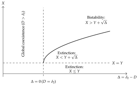
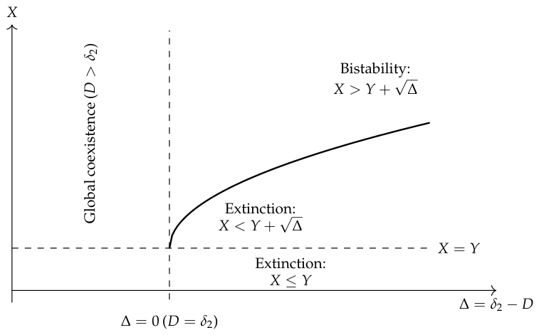
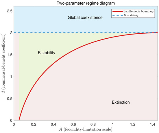
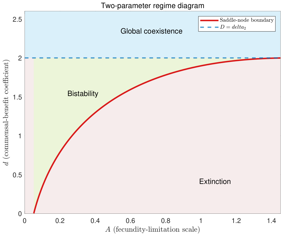
At this parameter value, $X=Y+\sqrt{{\Delta }_{\mathrm{SN}}}$, and the two positive equilibria coalesce at $x_2=x_{\mathrm{crit}}$. The overall parameter regimes are summarized in Figure 2.

Figure 2. Regime diagram in the $(\Delta ,X)$-plane for fixed Y (schematic, drawn with $Y=\sqrt{0.5}$). For $\Delta <0$ (i.e., $D>{\delta }_2$), the unique positive equilibrium is globally asymptotically stable (Theorem 2). For $\Delta >0$, the curve $X=Y+\sqrt{\Delta }$ separates the bistable regime (two positive equilibria, Theorem 4) from the extinction regime (no positive equilibrium, Theorem 5); in the region $X\le Y$, the extinction regime extends to the entire half-plane $\Delta >0$. On the curve, a non-degenerate saddle-node bifurcation occurs (Theorem 7).

Proposition 2. 

Assume $D<{\delta }_2$ and $X=Y+\sqrt{\Delta }$. The limiting planar system has the origin as a hyperbolic sink and one positive saddle-node equilibrium $E_3^{\mathrm{SN}}$. On its one-dimensional center manifold, the reduced equation is locally equivalent, after orientation-preserving changes of variables and time, to

$$\dot{u}=-c{u}^2+O\left(u^3\right),c>0.$$

Thus, the double equilibrium is semistable: initial points on one side approach it, whereas those on the other side leave its neighborhood toward extinction. The strict global-extinction result of Theorem 5 does not include this equality case. In the full system, points in the stable set may converge to $E_3^{\mathrm{SN}}$; all other biologically meaningful points converge to $E_1$.

Proof. 

At equality, the equilibrium polynomial has a double root $x_2=x_{\mathrm{crit}}>0$, and the planar Jacobian has one zero and one negative eigenvalue. The quadratic coefficient computed explicitly in Theorem 7 is nonzero and negative under the chosen center orientation, giving the displayed normal form. The phase-line conclusion follows. Boundedness, absence of cycles and asymptotic autonomy then leave only $E_1$ and $E_3^{\mathrm{SN}}$ as full-system limits.    □

Theorem 7. 

Assume $X>Y$ and ${\delta }_2>{(X-Y)}^2$, and set

$$D_{\mathrm{SN}}={\delta }_2-{(X-Y)}^2\in (0,{\delta }_2).$$

Then, system (3) undergoes a non-degenerate saddle-node bifurcation at $D=D_{\mathrm{SN}}$.

Proof. 

At $D=D_{\mathrm{SN}}$, Equation (16) has a double positive root at $x_2=x_{\mathrm{crit}}$, the planar Jacobian has a simple zero eigenvalue, the remaining planar eigenvalue is

$$-C_1=-\left((\beta +{\delta }_1)+2\gamma x_{\mathrm{crit}}+{\Delta }_{\mathrm{SN}}\right)<0,$$

and the host eigenvalue is $-b_2<0$. By the center manifold theorem, the bifurcation is governed by the one-dimensional center direction of the planar limiting system, the host direction playing no role. Taking $\mu =D-D_{\mathrm{SN}}$, let w and v be right and left null vectors of the planar Jacobian, as specified in Appendix A. The two standard Sotomayor conditions [45] are explicitly

$$v^T{F}_{\mu }=x_{\mathrm{crit}}>0,v^T{D}_x^{2}F(w,w)=-2\gamma {\displaystyle \frac{x_{\mathrm{crit}}}{x_{\mathrm{crit}}+A}}\ne 0.$$

The first gives parameter transversality and the second quadratic non-degeneracy. Thus, the bifurcation is a non-degenerate saddle-node. These vector-field conditions are the coordinate-invariant formulation of the required nonzero parameter and second-state derivatives.    □

Remark 2. 

The parameter D is a composite quantity. In practice, the bifurcation is realized by varying the commensal benefit coefficient d: since

$$D\left(d\right)={\displaystyle \frac{d{y}^{*}}{{\eta }_1+{\eta }_2{y}^{*}}}$$

is strictly increasing in d, the threshold $D=D_{\mathrm{SN}}$ corresponds uniquely to

$$d_{\mathrm{SN}}={\displaystyle \frac{D_{\mathrm{SN}}({\eta }_1+{\eta }_2{y}^{*})}{y^{*}}}.$$

The bifurcation is physically realizable only when $D_{\mathrm{SN}}>0$, i.e., ${\delta }_2>{(X-Y)}^2$; otherwise, the threshold lies outside the admissible range $D\in (0,{\delta }_2)$ of the weak-benefit case. For $X\le Y$, no positive branch exists in that case and the saddle-node mechanism is absent.

7. Numerical Illustrations

The computations in this section use illustrative, scaled values, not parameter estimates for a particular ecological system. Their purpose is to verify the analytical boundaries, visualize basin dependence, and to test the robustness of the mechanism under parameter variation.

We fix

$$\alpha =3,\beta =1,{\delta }_1=1,\gamma =1,b_2=1,a_2=1,{\eta }_1=1,{\eta }_2=1,A=0.5.$$

Then, $y^{*}=1$, $X=\sqrt{3/2}\approx 1.225$, $Y=\sqrt{0.5}\approx 0.707$, and ${(X-Y)}^2\approx 0.268$.

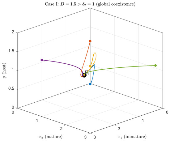
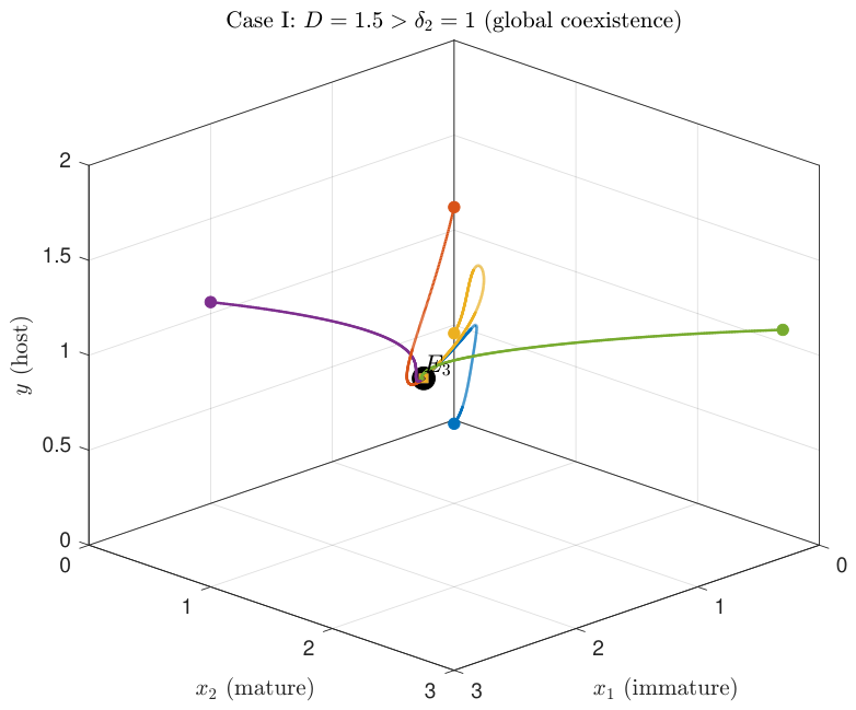
Consider ${\delta }_2=1$ and $d=3$, so $D=3/2=1.5>{\delta }_2$. The equilibrium equation is $2x_2^2-3x_2-0.5=0$, giving $E_3\approx (1.90,1.65,1)$. By Theorem 2, this equilibrium is globally asymptotically stable; Figure 3 shows the convergence of typical trajectories.

Figure 3. Case I: $D=1.5>{\delta }_2$. All positive-host solutions with $x_2\left(0\right)\ge 0$, $x_1\left(0\right)+x_2\left(0\right)>0$, and $y\left(0\right)>0$ converge to the unique coexistence equilibrium.

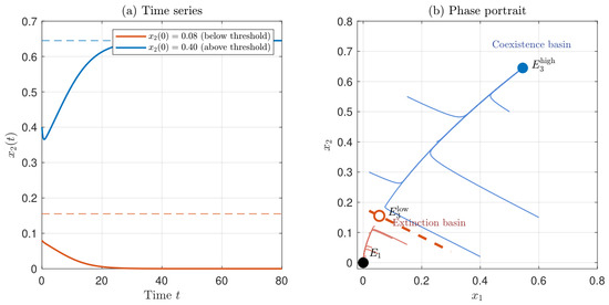
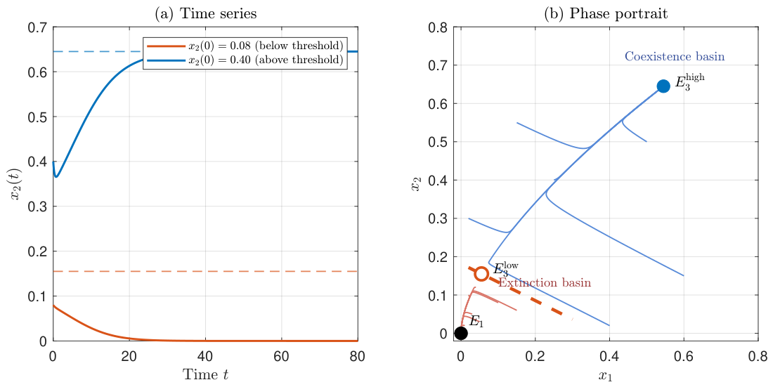
Take ${\delta }_2=1$ and $d=1.6$, so $D=0.8$ and $\Delta =0.2<{(X-Y)}^2$. The quadratic is $2x_2^2-1.6x_2+0.2=0$, with roots $x_{2,\mathrm{small}}^{**}\approx 0.155$ and $x_{2,\mathrm{large}}^{**}\approx 0.645$. Hence,

$$E_3^{\mathrm{low}}\approx (0.055,0.155,1),E_3^{\mathrm{high}}\approx (0.545,0.645,1).$$

The low-density equilibrium is a saddle, whereas $E_1$ and $E_3^{\mathrm{high}}$ are locally asymptotically stable; the phase portrait shown in Figure 4 displays the two basins separated by the stable manifold of the saddle, in agreement with Theorem 6.

Figure 4. Case II bistable regime: $D=0.8$ and $\Delta =0.2$. The stable manifold of the saddle $E_3^{\mathrm{low}}$ is a one-dimensional separatrix separating the extinction basin from the coexistence basin (Theorem 6). (a) Time series; (b) Phase portrait.

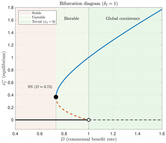
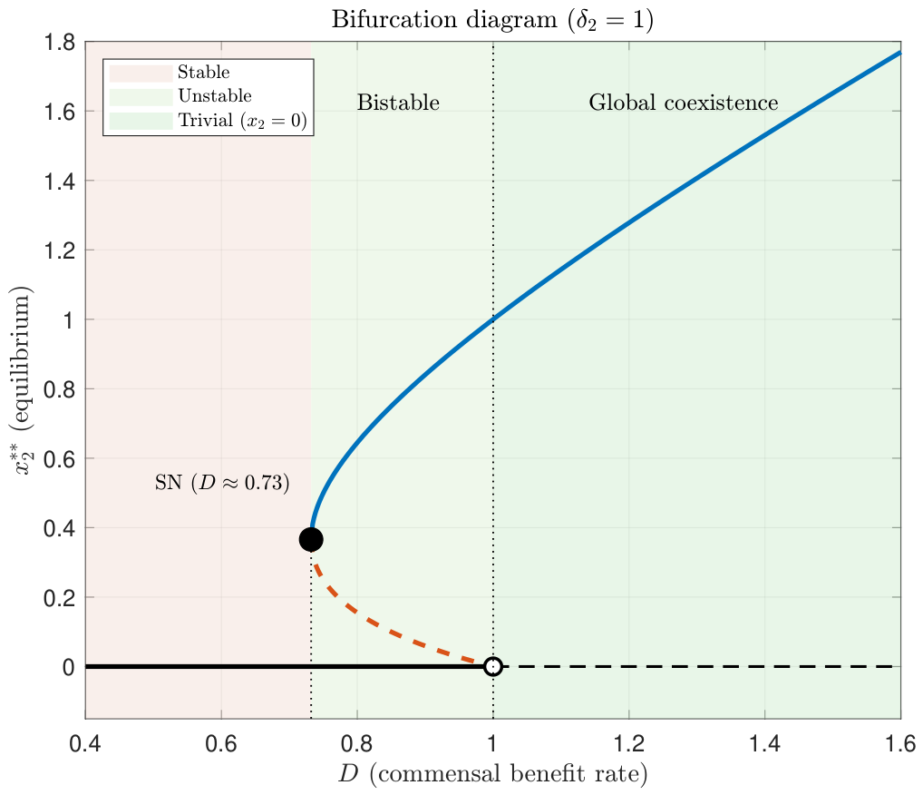
Keeping the other parameters fixed, let D vary. The equilibrium equation is $2x_2^2-2D{x}_2+(1-D)=0$, whose roots are

$$x_2^{\pm }\left(D\right)={\displaystyle \frac{D\pm \sqrt{D^2+2D-2}}{2}}.$$

The saddle-node bifurcation occurs at $D=D_{\mathrm{SN}}=1-{(X-Y)}^2\approx 0.732$, where $x_2=x_{\mathrm{crit}}\approx 0.366$. For $D_{\mathrm{SN}}<D<1$, the system is bistable; for $D<D_{\mathrm{SN}}$, there is no positive equilibrium and the commensal species goes extinct; for $D>1$, there is global coexistence. Figure 5 shows the resulting bifurcation diagram, in which the saddle-node point at $D_{\mathrm{SN}}\approx 0.732$ and the boundary equilibrium exchange at $D={\delta }_2=1$ are the two codimension-one events predicted by Theorem 7 and the discussion in Section 6.

Figure 5. Bifurcation diagram of the mature commensal equilibrium $x_2^{**}$ as D varies. Solid curves denote stable equilibria and dashed curves denote unstable equilibria. The saddle-node point occurs at $D_{\mathrm{SN}}\approx 0.73$ and the boundary equilibrium exchange at $D={\delta }_2=1$.

To assess robustness beyond a one-parameter continuation, we next vary the fecundity-limitation scale A and the primitive benefit coefficient d. Since

$$D\left(d\right)={\displaystyle \frac{d{y}^{*}}{{\eta }_1+{\eta }_2{y}^{*}}},Y\left(A\right)=\sqrt{\gamma A},$$

the analytical saddle-node boundary is

$$D\left(d\right)={\delta }_2-{\left(\sqrt{{\displaystyle \frac{\alpha \beta }{\beta +{\delta }_1}}}-\sqrt{\gamma A}\right)}^2,$$

where the right-hand side is positive and $X>Y$. Figure 6 classifies a two-dimensional parameter region directly from these inequalities. It confirms that increasing A expands the extinction region, whereas increasing d first creates bistability and ultimately gives global coexistence after $D={\delta }_2$.

Figure 6. Two-parameter regime diagram in the $(A,d)$-plane. The analytical curves distinguish extinction, bistability and global coexistence. Parameter values not shown are those used in the preceding simulations.

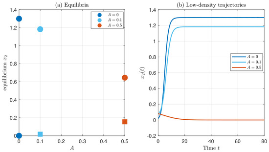
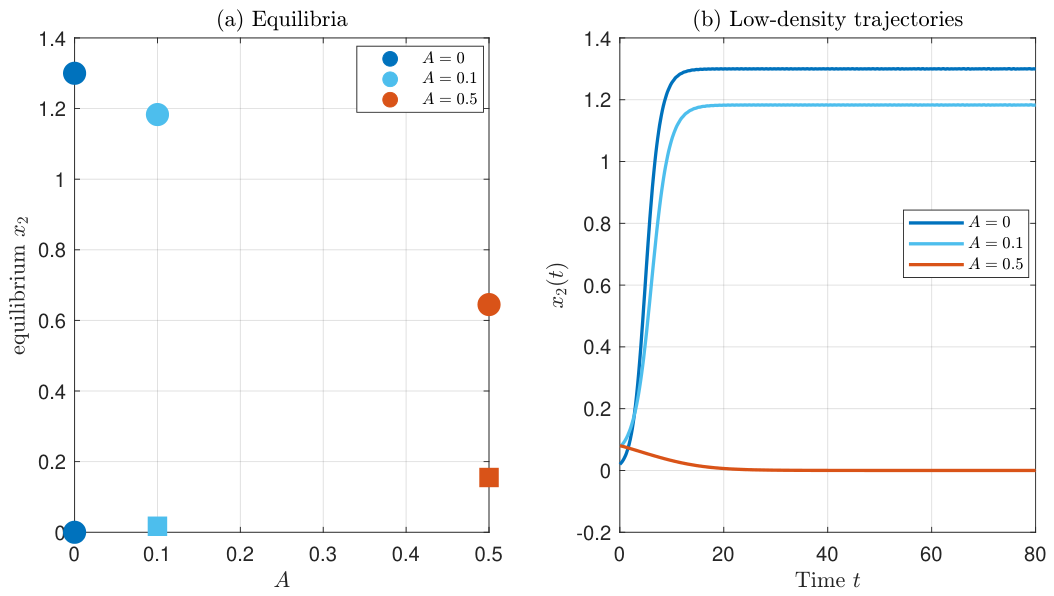
A direct comparison with the inherited model is shown in Figure 7. At $A=0$, recruitment is linear and the fecundity-induced pair of positive equilibria is absent. A small positive A creates a component Allee effect and a corresponding saddle-node branch; a larger A raises the effective barrier $Y=\sqrt{\gamma A}$, shifts the saddle-node threshold toward greater host benefit, and enlarges the range of initial conditions leading to extinction. This comparison isolates the nonlinear recruitment term as the mechanism responsible for the new dynamics.

Figure 7. Direct numerical comparison of linear recruitment ($A=0$) and fecundity-limited recruitment at two positive values of A. Stable equilibria are marked with circles and unstable equilibria with squares. (a) Equilibria; (b) Low density trajectories.

The threshold formula also provides a transparent sensitivity summary. Increasing $\alpha$ increases reproductive capacity X. Increasing $\beta$ increases X with a saturating effect through $\beta /(\beta +{\delta }_1)$, whereas increasing ${\delta }_1$ reduces it. Increasing A or $\gamma$ raises Y, increasing ${\delta }_2$ raises Δ, and increasing d lowers Δ through D. Numerical sweeps over these parameters reproduce the same three analytical regimes and show that the conclusions are not tied to the single baseline parameter set.

For reproducibility, we computed all trajectories using MATLAB’s adaptive fifth-order Runge–Kutta solver ode45, using relative tolerance 10⁻⁹ and absolute tolerance 10⁻¹¹. The time intervals are those reported in the figure-generating script generate_improved_figures.m. The planar separatrix in Figure 4 was approximated by bisection in the initial mature-density coordinate; each trial trajectory was integrated to time 150, and the bisection was stopped after 40 iterations. The bifurcation curves were computed directly from the explicit quadratic roots, not inferred from numerical continuation. Figure 6 and Figure 7 were likewise generated from the analytical equilibrium formulas and the same ode45 tolerances. These computations are illustrative and reproducible, but they are not empirical validation of the model.

8. Concluding Remarks

We have shown how a birth-related weak Allee effect changes the qualitative behavior of a stage-structured commensalism model with Holling type II benefit. The main threshold quantities are

$$X=\sqrt{{\displaystyle \frac{\alpha \beta }{\beta +{\delta }_1}}},Y=\sqrt{\gamma A},\Delta ={\delta }_2-D.$$

Here, X measures the effective reproductive capacity of the commensal species, Y the combined Allee and density-regulation intensity, and $\Delta$ the deficit between mature mortality and host-provided benefit.

Three regimes emerge. When $D>{\delta }_2$, there is a single positive equilibrium which attracts every biologically meaningful solution; the commensal benefit is strong enough to overcome low-density depression. When $D<{\delta }_2$ and $X>Y+\sqrt{\Delta }$, two positive equilibria coexist, producing bistability between extinction and coexistence, and the low-density saddle acts as an Allee threshold. When $D<{\delta }_2$ and $X<Y+\sqrt{\Delta }$, no positive equilibrium exists and the commensal species is driven to extinction. On the separating curve $X=Y+\sqrt{\Delta }$, the two equilibria merge in a saddle-node bifurcation.

A key consequence is that a weak Allee effect at the birth level, $f\left(x\right)/x\to 0$ as $x\to 0^{+}$, translates into strong Allee-type threshold behavior at the population level: the low-density equilibrium is unstable and separates the basins of extinction and coexistence. This parallels the observation of Lin [6] that Allee effects need not always be detrimental. The possible relevance to conservation should be interpreted only as a modeling implication: the present analysis does not provide empirical evidence that a particular real commensal population has this threshold.

From a modeling perspective, the only structural change is the introduction of nonlinear recruitment. Nevertheless, it creates bistability and a saddle-node bifurcation that are absent in the linear-recruitment model [25]. Similar mechanisms may operate in other host–commensal or density-dependent recruitment systems, and their study in discrete-time or stochastic settings appears to be a natural continuation.

The conclusions should be interpreted in light of the triangular model assumption. Strict commensalism is represented by complete absence of feedback from the commensal to the host, so $y\left(t\right)$ converges independently and the long-term problem becomes planar. This simplification is biologically reasonable when the commensal’s effect on a large host population is negligible, but it is also essential to the present global proofs. If weak positive or negative feedback were added to the host equation, the limiting reduction would generally be lost; equilibrium thresholds and basin boundaries could shift, and genuinely three-dimensional oscillatory dynamics could no longer be excluded by the present Dulac argument. Environmental stochasticity, delay, spatial structure and calibration to a named host–commensal system are therefore important directions for future work.

Use of AI Tools Declaration

During revision, the authors used a generative artificial-intelligence assistant to help organize reviewer comments, suggest language revisions and check the presentation of mathematical arguments. The authors independently verified every equation, proof, reference, figure and scientific claim; they made all final editorial decisions and accept full responsibility for the content.

References

- Odum, E.P. Fundamentals of Ecology; W. B. Saunders: Philadelphia, PA, USA, 1953. [Google Scholar]
- Bronstein, J.L. Our current understanding of mutualism. Q. Rev. Biol. 1994, 69, 31–51. [Google Scholar] [CrossRef] [Scilit] [PubMed]
- Bruno, J.F.; Stachowicz, J.J.; Bertness, M.D. Inclusion of facilitation into ecological theory. Trends Ecol. Evol. 2003, 18, 119–125. [Google Scholar] [CrossRef] [Scilit]
- Chen, B. Dynamic behaviors of a commensal symbiosis model involving Allee effect and one party can not survive independently. Adv. Differ. Equ. 2018, 2018, 212. [Google Scholar] [CrossRef] [Scilit]
- Wu, R.; Li, L.; Lin, Q. A Holling type commensal symbiosis model involving Allee effect. Commun. Math. Biol. Neurosci. 2018, 2018, 6. [Google Scholar] [CrossRef] [Scilit]
- Lin, Q. Allee effect increasing the final density of the species subject to the Allee effect in a Lotka–Volterra commensal symbiosis model. Adv. Differ. Equ. 2018, 2018, 196. [Google Scholar] [CrossRef] [Scilit]
- Lei, C. Dynamic behaviors of a Holling type commensal symbiosis model with the first species subject to Allee effect. Commun. Math. Biol. Neurosci. 2019, 2019, 3. [Google Scholar] [CrossRef] [Scilit]
- Chong, Y.; Kashyap, A.J.; Chen, S.; Chen, F. Dynamics analysis of a discrete-time commensalism model with additive Allee effect for the host species. Axioms 2023, 12, 1031. [Google Scholar] [CrossRef] [Scilit]
- Zhong, J.; Chen, L.; Chen, F. Stability and bifurcation in a two-patch commensal symbiosis model with nonlinear dispersal and additive Allee effect. Int. J. Biomath. 2026, 19, 2450099. [Google Scholar] [CrossRef] [Scilit]
- He, X.; Zhu, Z.; Chen, J.; Chen, F. Dynamical analysis of a Lotka–Volterra commensalism model with additive Allee effect. Open Math. 2022, 20, 646–665. [Google Scholar] [CrossRef] [Scilit]
- Zhang, J.; Yue, Q. Dynamical behavior of a host–commensal system with multiplicative Allee effect and non-selective harvesting. Electron. Res. Arch. 2026, 34, 6404–6431. [Google Scholar] [CrossRef] [Scilit]
- Chen, B. The influence of commensalism on a Lotka–Volterra commensal symbiosis model with Michaelis–Menten-type harvesting. Adv. Differ. Equ. 2019, 2019, 43. [Google Scholar] [CrossRef] [Scilit]
- Liu, X.; Yue, Q. Stability property of the boundary equilibria of a symbiotic model of commensalism and parasitism with harvesting in commensal populations. AIMS Math. 2022, 7, 18793–18808. [Google Scholar] [CrossRef] [Scilit]
- Chen, F.; Chen, Y.; Li, Z.; Chen, L. Note on the persistence and stability property of a commensalism model with Michaelis–Menten harvesting and Holling Type II commensalistic benefit. Appl. Math. Lett. 2022, 134, 108381. [Google Scholar] [CrossRef] [Scilit]
- Jawad, S. Study the dynamics of commensalism interaction with Michaelis–Menten-type prey harvesting. Al-Nahrain J. Sci. 2022, 25, 45–50. [Google Scholar] [CrossRef] [Scilit]
- Puspitasari, N.; Kusumawinahyu, W.M.; Trisilowati, T. Dynamical analysis of the symbiotic model of commensalism in four populations with Michaelis–Menten-type harvesting in the first commensal population. J. Teor. Apl. Mat. 2021, 5, 392–404. [Google Scholar]
- Xu, L.; Xue, Y.; Xie, X.; Lin, Q. Global attractivity of symbiotic model of commensalism in four populations with Michaelis–Menten-type harvesting in the first commensal populations. Axioms 2022, 11, 337. [Google Scholar] [CrossRef] [Scilit]
- Su, Q.; Zhang, Z.; Chen, F. Dynamics of a discrete commensalism model with non-selective harvesting: Dependence on the harvestable proportion. J. Appl. Anal. Comput. 2026, 17, 105–118. [Google Scholar] [CrossRef] [Scilit] [PubMed]
- Xu, L.; Xue, Y.; Xie, X.; Lin, Q. Dynamic behaviors of an obligate commensal symbiosis model with Crowley–Martin functional responses. Axioms 2022, 11, 298. [Google Scholar] [CrossRef] [Scilit]
- Jiang, Q.; Liu, Z.; Wang, Q.; Tan, R.; Wang, L. Two delayed commensalism models with noise coupling and interval biological parameters. J. Appl. Math. Comput. 2022, 68, 979–1011. [Google Scholar] [CrossRef] [Scilit]
- Sanchez-Palencia, E.; Françoise, J.-P. On predation–commensalism processes as models of bi-stability and constructive role of systemic extinctions. Acta Biotheor. 2021, 69, 497–510. [Google Scholar] [CrossRef] [Scilit] [PubMed]
- Tassaddiq, A.; Ahmed, R.; Ditta, A. Exploring stability and bifurcation in a discretized commensalism model. Nonlinear Dyn. 2025, 113, 28463–28475. [Google Scholar] [CrossRef] [Scilit]
- Shofiyya, N.; Kusumawinahyu, W.M.; Habibah, U. Model of three species commensalism–amensalism symbiosis with Beddington–DeAngelis functional responses. CAUCHY J. Mat. Murni Apl. 2025, 10, 1054–1068. [Google Scholar] [CrossRef] [Scilit]
- Li, X.; Yue, Q.; Chen, F. Global stability and bifurcation of a three-species commensalism–amensalism model with Beddington–DeAngelis functional response. Axioms 2026, 15, 495. [Google Scholar] [CrossRef] [Scilit]
- Chen, F.; Li, Z.; Chen, L. Dynamic behaviors of a stage structure commensalism system with Holling Type II commensalistic benefits. WSEAS Trans. Math. 2022, 21, 810–824. [Google Scholar] [CrossRef] [Scilit]
- Aiello, W.G.; Freedman, H.I. A time-delay model of single-species growth with stage structure. Math. Biosci. 1990, 101, 139–153. [Google Scholar] [CrossRef] [Scilit] [PubMed]
- Allee, W.C. Co-operation among animals. Am. J. Sociol. 1931, 37, 386–398. [Google Scholar] [CrossRef] [Scilit] [PubMed]
- Courchamp, F.; Clutton-Brock, T.; Grenfell, B. Inverse density dependence and the Allee effect. Trends Ecol. Evol. 1999, 14, 405–410. [Google Scholar] [CrossRef] [Scilit] [PubMed]
- Stephens, P.A.; Sutherland, W.J. Consequences of the Allee effect for behaviour, ecology and conservation. Trends Ecol. Evol. 1999, 14, 401–405. [Google Scholar] [CrossRef] [Scilit] [PubMed]
- Berec, L.; Angulo, E.; Courchamp, F. Multiple Allee effects and population management. Trends Ecol. Evol. 2007, 22, 185–191. [Google Scholar] [CrossRef] [Scilit] [PubMed]
- Kramer, A.M.; Dennis, B.; Liebhold, A.M.; Drake, J.M. The evidence for Allee effects. Popul. Ecol. 2009, 51, 341–354. [Google Scholar] [CrossRef] [Scilit]
- Dennis, B. Allee effects: Population growth, critical density, and the chance of extinction. Nat. Resour. Model. 1989, 3, 481–538. [Google Scholar] [CrossRef] [Scilit]
- Lewis, M.; Kareiva, P. Allee dynamics and the spread of invading organisms. Theor. Popul. Biol. 1993, 43, 141–158. [Google Scholar] [CrossRef] [Scilit]
- Boukal, D.S.; Berec, L. Single-species models of the Allee effect: Extinction boundaries, sex ratios and mate encounters. J. Theor. Biol. 2002, 218, 375–394. [Google Scholar] [CrossRef] [Scilit] [PubMed]
- Elaydi, S.; Sacker, R. Population models with Allee effect: A new model. J. Biol. Dyn. 2010, 4, 397–408. [Google Scholar] [CrossRef] [Scilit] [PubMed]
- Drake, J.M.; Kramer, A.M. Allee effects. Nat. Educ. Knowl. 2011, 3, 2. [Google Scholar] [CrossRef] [Scilit]
- Taylor, C.M.; Hastings, A. Allee effects in biological invasions. Ecol. Lett. 2005, 8, 895–908. [Google Scholar] [CrossRef] [Scilit]
- Gascoigne, J.C.; Lipcius, R.N. Allee effects driven by predation. J. Appl. Ecol. 2004, 41, 801–810. [Google Scholar] [CrossRef] [Scilit]
- Friedenberg, N.A.; Powell, J.A.; Ayres, M.P. Synchrony’s double edge: Transient dynamics and the Allee effect in stage-structured populations. Ecol. Lett. 2007, 10, 564–573. [Google Scholar] [CrossRef] [Scilit] [PubMed]
- Lazaryan, N.; Sedaghat, H. Extinction and the Allee effect in an age structured Ricker population model with inter-stage interaction. Discret. Contin. Dyn. Syst.-B 2018, 23, 731–747. [Google Scholar] [CrossRef] [Scilit]
- Hao, P.; Wang, X.; Wei, J. Global Hopf bifurcation of a population model with stage structure and strong Allee effect. Contin. Dyn. Syst.-S 2017, 10, 973–993. [Google Scholar] [CrossRef] [Scilit]
- Jorge, D.C.P.; Martinez-Garcia, R. Demographic effects of aggregation in the presence of a component Allee effect. J. R. Soc. Interface 2024, 21, 20240042. [Google Scholar] [CrossRef] [Scilit] [PubMed]
- Thieme, H.R. Convergence results and a Poincaré–Bendixson trichotomy for asymptotically autonomous differential equations. J. Math. Biol. 1992, 30, 755–763. [Google Scholar] [CrossRef] [Scilit]
- Thieme, H.R. Asymptotically autonomous differential equations in the plane. Rocky Mt. J. Math. 1994, 24, 351–380. [Google Scholar] [CrossRef] [Scilit]
- Kuznetsov, Y.A. Elements of Applied Bifurcation Theory, 3rd ed.; Springer: New York, NY, USA, 2004. [Google Scholar]
Disclaimer/Publisher’s Note: The statements, opinions and data contained in all publications are solely those of the individual author(s) and contributor(s) and not of MDPI and/or the editor(s). MDPI and/or the editor(s) disclaim responsibility for any injury to people or property resulting from any ideas, methods, instructions or products referred to in the content. |
© 2026 by the authors. Licensee MDPI, Basel, Switzerland. This article is an open access article distributed under the terms and conditions of the Creative Commons Attribution (CC BY) license.