


Abstract
In this work, we prove the strong convergence of an inertial iterative scheme to approximate solutions of the equilibrium fixed point problem associated with nonexpansive mappings in Hilbert spaces. Numerical simulations are carried out to examine the performance of the proposed approach. The results indicate that the proposed inertial approach achieves faster convergence when compared with existing comparable iterative schemes. We also investigate how different choices of initial values influence the convergence behavior of our algorithms and we compare these effects with those observed in classical iterative schemes through graphical illustrations. In applications, we used our approach to solve the signal processing problem. We also apply it to a mathematical model describing the spread of an infectious disease, which illustrates its relevance to real-world dynamical systems. Finally, we show that the proposed method can be applied in solving constrained optimization, variational inequality and split feasibility problems which highlight its flexibility and wide applicability.
MSC:
47J25; 90C33; 65J15; 65K15
1. Introduction and Preliminaries
Many phenomena arising from science, economics and engineering can be expressed using mathematical equations. These equations serve as the foundation for constructing mathematical models that help explain, analyze, and predict the behavior of real-world systems. Depending on the nature of the problem, mathematical models may be linear or nonlinear, deterministic or stochastic and static or dynamic. In many situations, such models are expressed through differential or integral equations.
For a wide range of practical applications, dynamic systems can be formulated in terms of nonlinear Volterra integral equations. These equations frequently appear when an initial value problem is transformed into its equivalent integral form. In fact, many nonlinear integral equations are mathematically equivalent to systems of ordinary differential equations with given initial conditions. Obtaining exact solutions of nonlinear equations is often challenging and, in many cases, only approximate solutions can be obtained. To address this difficulty, several analytical and numerical techniques have been developed. Among these approaches, fixed point theory has proved to be a powerful tool for investigating the existence and approximation of solutions. Fixed point methods not only provide theoretical guarantees of solvability but also lead to effective iterative algorithms for computing solutions. A large number of problems arising in applied mathematics, engineering, and scientific computing can be expressed in terms of functional equations and inclusions, which in many cases can be transformed into equivalent fixed point formulations, making fixed point theory an effective tool for their analysis. Typical examples include optimization problems in artificial neural networks, epidemic and population dynamics models, and Nash equilibrium models in game theory.
Moreover, fixed point techniques play a crucial role in the analysis of iterative algorithms. As a result, fixed point theory continues to be a valuable mathematical tool for understanding and solving complex real-world problems across many disciplines. The study of nonexpansive mappings in iterative algorithms is important for several key reasons. First, the existence of fixed points for these particular mappings depends primarily on the geometric structure of spaces, rather than on compactness assumptions. This makes the theory applicable in a much broader setting. Second, nonexpansive mappings naturally arise as transition operators in certain initial value problems associated with differential inclusions. Third, many problems in applied mathematics and engineering lead to operator equations involving nonexpansive mappings. These include applications in optimization, compressed sensing, variational inequalities, and image restoration problems.
In what follows, we denote by a Hilbert space and let be a closed and convex set. The weak convergence and strong convergence of to are denoted by and , respectively. Moreover, the set of weak limits of is represented by .
Assume that and is a bifunction. The fixed point problem (FPP) given as: Find
The equilibrium problem (EP) of is given by:
The equilibrium fixed point problem (EFPP) can be expressed as follows: Find
The set of all solutions of the EFPP is denoted by . Many nonlinear problems become particular cases of the EFPP. It encompasses equilibrium problems, variational inequalities, optimization and complementarity problems, classical fixed point problems, and Nash equilibrium problems. For further details and related discussions, see, for example, refs. [1,2,3,4].
The Banach contraction principle leads to a simple iterative procedure for approximating fixed points, commonly known as the Picard iteration scheme. This method is based on repeatedly applying a contraction mapping starting from an initial approximation. Through successive iterations, the generated sequence converges to the unique fixed point of the mapping under certain contraction conditions. The Picard scheme may not converge for nonexpansive mappings. To achieve this goal, Mann iterative scheme [5] was proposed which is given as follows:
where .
Now, the Ishikawa iteration [6] can be defined as follows:
here .
A three step iteration process defined by Noor [7] is given by:
where , .
Later on Agarwal [8] introduced the following iterative scheme and is given as:
here .
An iterative sequence generated by Abbas et al., scheme [9] is given as follows:
here .
Moreover, the Thakur et al. scheme [10] is defined as follows:
The M-iteration [11] given by
Abbas et al. [12] proposed the AA-iterative to approximate the fixed points and is given by:
here .
Recently, Sharma and Chandok [13] defined the following fixed point iterative scheme:
For the common solution of equilibrium problem, variational inclusion and fixed point problem the Alakoya scheme was proposed in [14] and is define as:
Find such that
where and are nonexpansive mappings.
In this paper, we propose an inertial-viscosity iterative scheme for approximating a common solution of the EP and the FPP. Most of the existing schemes discussed above converge only weakly to a fixed point of a given mapping. Although the scheme presented in [13] achieves strong convergence under certain assumptions, it approximates the solutions of EP and FPP separately. On the other hand, our proposed scheme incorporates an inertial term, which helps accelerate the convergence process and is capable of approximating a unified solution of both the EP and FPP simultaneously.
Remark 1.
The main contribution of this work is the development of an inertial viscosity type iterative framework to approximate solutions of equilibrium fixed point problems associated with nonexpansive mappings. The proposed scheme combines an inertial extrapolation step with a viscosity approximation mechanism with the equilibrium problem. This combination provides a unified framework that allows the equilibrium condition and the fixed point constraint deal simultaneously. More precisely, under suitable assumptions on the bifunction, the nonexpansive mapping, and the control parameters, we establish the strong convergence of the generated sequence to a solution of the equilibrium fixed point problem. The proposed framework also contains several existing iterative procedures as particular cases through appropriate choices of the parameters and operators. Furthermore, the theoretical framework is applied to nonlinear integral equations, signal reconstruction, constrained optimization, and split feasibility problems, illustrating the applicability of the proposed approach to different classes of problems involving nonexpansive mappings.
Following is our proposed iterative scheme:
Set , where
Then find
Find such that,
where
- (i)
- lie in also with .
- (ii)
- , where .
- (iii)
- is fixed and such that
- (iv)
- such that
Remark 2.
Observe that
Lemma 1
([15]). If is nonexpansive, then is demiclosed on , that is, for every sequence in with and gives for each .
Now we recall that:
Definition 1.
The map known as weakly lower semicontinuous at if for each in such that we get
Lemma 2
([16]). If and then we have the following:
- (i)
- ,
- (ii)
- ,
- (iii)
- ,
- (iv)
- .
Lemma 3
([17]). If and with then we have:
Lemma 4
([18]). Assume and , , with the following:
- (i)
- Assume for we have is bounded.
- (ii)
- Assume and then we have .
Lemma 5
([19]). Suppose that , with , and
If for each subsequence of with Then we have
2. Main Results
In this section, we present the convergence of our proposed inertial iterative scheme to approximate solutions of equilibrium fixed point problem of nonexpansive mappings in the framework of Hilbert spaces.
Let us start with the following assumptions on the bifunction .
Assumption 1.
Suppose that satisfies the following:
- , for all .
- for all .
- , for all .
- For each , is lower semi-continuous and convex.
Definition 2.
Fix , define as follows:
Remark 3.
The bifunction plays a central role to incorporate the equilibrium condition into the proposed equilibrium fixed point problem. The choice of U determines the equilibrium component of the problem. Several important problems can be represented by suitable choices of . For example, if is a monotone operator, then
satisfies Assumption 1. In particular, on , taking gives and the corresponding equilibrium problem has the solution . Another nontrivial example is
where is a proper lower semicontinuous convex function. This choice also satisfies Assumption 1 and the associated equilibrium problem corresponds to minimizing ϕ over .
For the special case , the equilibrium condition is satisfied for every and every . Hence, the equilibrium problem imposes no additional restriction and the equilibrium fixed point problem reduces to the ordinary fixed point problem for . Moreover, from Definition 2, becomes the identity mapping. Consequently, the case shows that the proposed method contains the classical fixed point problem as a special case, whereas nonzero choices of allow the scheme to handle a genuine equilibrium constraint simultaneously with the fixed point constraint.
Lemma 6
([20]). Under the assumptions , we have
- is single-valued, firmly nonexpansive.
- The fixed point set of is solution of EP.
- The fixed point set of is closed and convex set.
Theorem 1.
Suppose that and are nonexpansive and contraction mappings, respectively. If fulfils . Then, sequence defined in (10) converges to an element in .
We divide the proof of the above theorem into the following Lemmas.
Lemma 7.
Under the assumptions of Theorem 1, the sequence given in (10) is bounded.
Proof.
Since is a contraction, so there is an element such that and This implies that .
As , we have
Now
By Remark 2, . We have as:
So, by Equation (13) we obtain
By (10), we get
Using (15), we have
From (10), we get that
Now using (16) and (17), we obtain that
Finally, using (14) and (18), we have
where If we put and . Then, using the Lemma 4 and the assumption on the parameters, we get is bounded, and hence is bounded. Further, and are also bounded. □
Lemma 8.
For a sequence generated in (10) and , we have the following inequality
Proof.
For , we get
where .
Also,
By (21), we obtain,
Using (22), we get
Finally,
Now by (20), (22)–(24), we have
Thus,
where }. □
Lemma 9.
Let be the sequence generated in (10) with holds. Then , where .
Proof.
Consider . Then we have
So by (25) we have
Now, we show () converges to zero. For this, we will use Lemma 5 by setting } and
and show that
for any subsequence of such that
From (26), we have
Using and (27) we have we obtain
Hence, we have
Similarly from (27) we get
and
By Remark 2, we get
Note that,
and
By (28) we get
Similarly, using (29) we have
By (30) and (31), we obtain that
From (30), (31), (34), (36) and (37), we get
Finally by (38), we have
We now prove . For this, we claim that . As is bounded, is nonempty. We may take and a subsequence of with as . So, by (32) and (33) we have and as . By the definition of , we have that
Here, using monotonicity of we get
As , using (28) and condition , we get,
Let where and . This gives , and by (40) we get .
Using , we get,
Hence, we have . As , then , gives . So, we have . Now, we want to show , using (33) and (34), we have and as . By nonexpansivness of S and demiclosedness principle, we have that . Consequently, . Also, using (33) and (34), we have = . Here, boundedness of gives a subsequence of such that and . Since , so we get
Using (39) and (42), we get
Since, by (26), we have
If we apply Lemma 5 on (44) and use (43), and , then we have . □
3. Numerical Computations
In this section, we provides the numerical experiments to illustrate the convergence of the proposed iterative algorithm. All simulations were implemented in MATLAB (version R2018a).
Example 1 presents a comparison among the proposed scheme and some known fixed point approaches in terms of convergence behavior.
Example 1.
Let be defined as follows
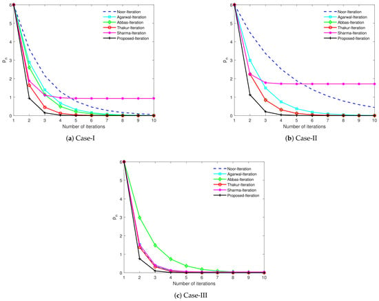
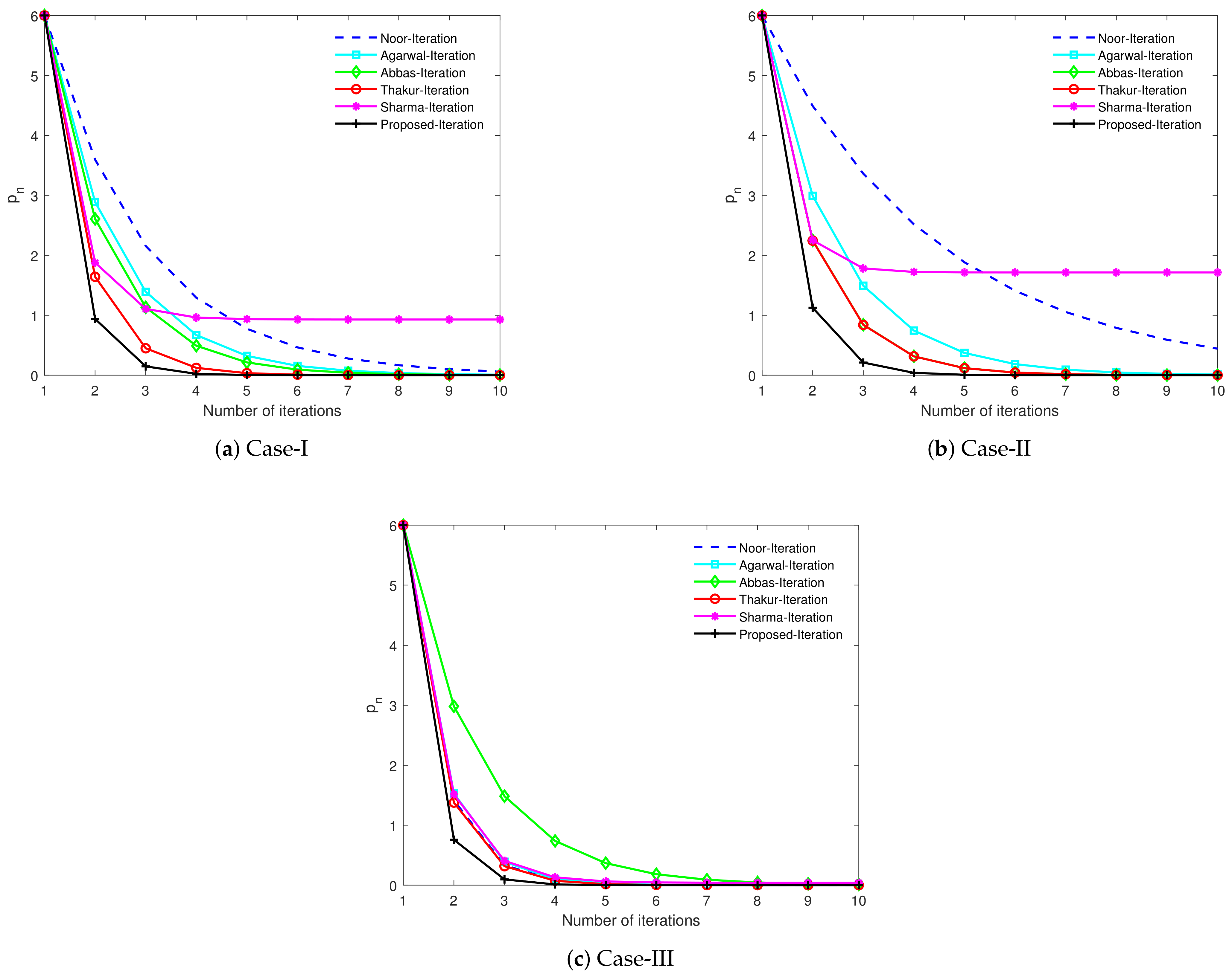
and . For the sake of comparison, we take equal initial values given by . Indeed, comparative algorithms has only one initial guess. We consider two cases and perform 10 iterations in each case, in case-I, we use , , and , in case-II, we use , , and and in case-III, we use , . Figure 1 shows the convergence behavior of different iterative methods and observe that the proposed scheme convergence faster than the existing comparable schemes considered herein.
Figure 1.
Performance comparison for different cases in Example 1.
Remark 4.
Note that, if , then satisfies
Thus, the proposed iteration method reduces to the viscosity type AA-iteration which will be used for the comparison with other iterative methods to approximate the fixed point.
Example 2.
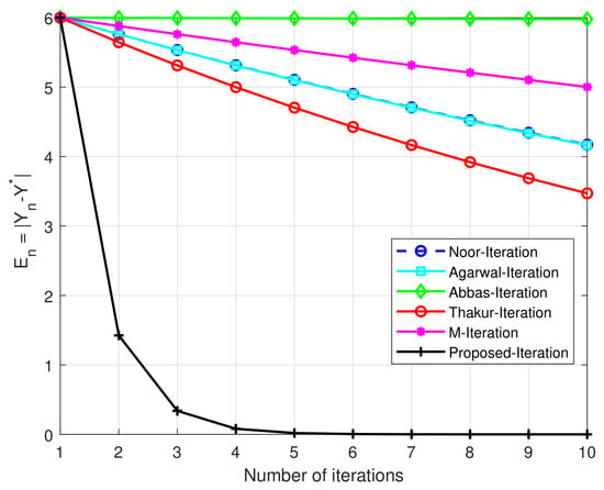
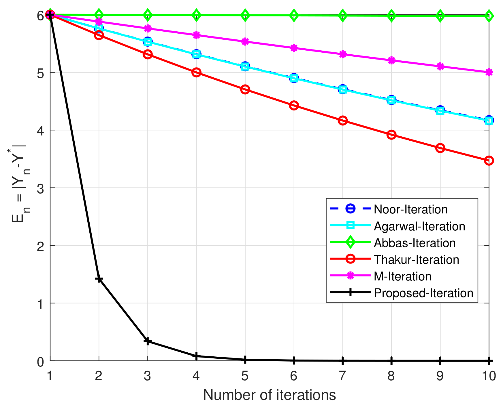
To further demonstrate the applicability of the proposed method to nonexpansive mappings, consider the mapping defined by Since has a fixed point which is 0. We take and . The remaining parameters are chosen as given in Example 1 case-III, the stopping criterion is From Figure 2, the numerical results demonstrate the convergence of the proposed scheme perform well in case of nonexpansive mapping.
Figure 2.
Performance comparison for error in Example 2.
Example 3.
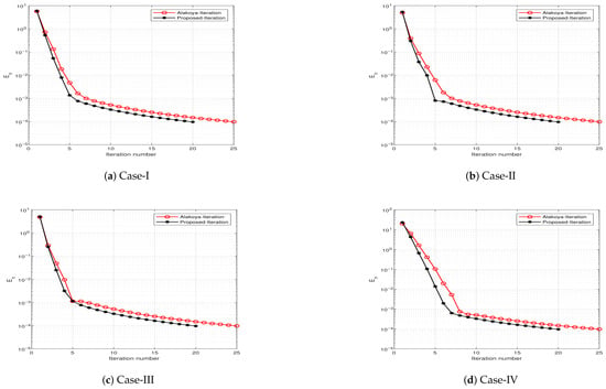
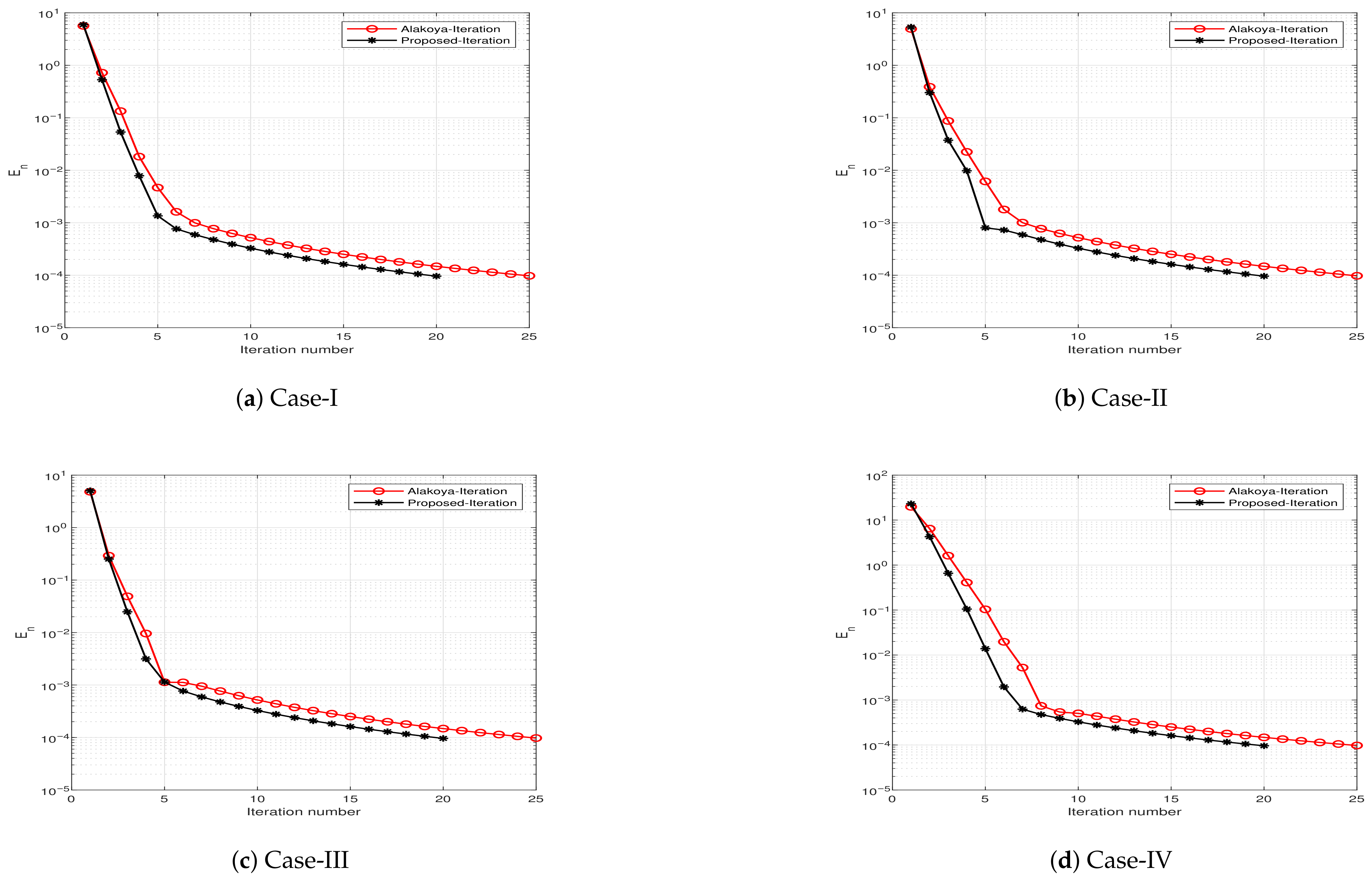
Let For a fixed vector a and define . Take , , , and . Fix , then . In this example, we will use and and choose different initial guesses in each case.
In case-I, we use , , in case-II, we use , , In case-III, we use , , and in case-IV, we use , . We use stopping criteria and . We now display versus the number of iterations in each case.The convergence behavior can be observed in Figure 3. Note that, the proposed iterative scheme performs well.
Figure 3.
Performance comparison for different cases in Example 3.
Remark 5.
Note that, the Alakoya iteration was employed for approximating the solution of equilibrium, split variational inclusion and fixed point problems. However, in our case we are considering equilibrium and fixed point problem, for the sake of numerical computations and comparison, we take in this Alakoya’s iteration scheme and compare it with our proposed scheme.
4. Applications
Here, we present some applications of the main result presented in the Section 2.
4.1. Application to Signal Processing
Fixed point iteration methods are widely used in modern signal processing applications, including signal restoration, noise reduction, image reconstruction, and adaptive filtering. In many real-world problems, obtaining the original signal from noisy or incomplete measurements can be modeled as finding a fixed point of an appropriate nonlinear operator.
We in this section, we study the effectiveness of proposed inertial viscosity iterative algorithm for signal reconstruction. Numerical experiments are carried out to examine its convergence behavior and reconstruction quality. The results are compared with Thakur iteration [10], M iteration [11], and AA-iterative method [12].
Let be the N-dimensional Euclidean space endowed with the standard norm . We consider a reference signal sampled on a uniform interval which is given by
where the frequencies of sinusoidal components are chosen as Hz and Hz.
To simulate measurement errors, noise is added to the original signal. The resulting observed signal is expressed as
where is a Gaussian random vector with distribution , and the parameter determines the level of noise contamination in the data.
For the purpose of signal recovery, we introduce a nonlinear mapping defined as
where represents a smoothing mechanism based on a moving-average filter. This mapping balances two objectives: preserving information from the noisy observation q and reducing noise through local averaging.
Consequently, the signal reconstruction task can be formulated to find the fixed point of , that is,
Furthermore, we employ the contraction operator h given by
Use the initial approximation , take , in our proposed inertial viscosity algorithm given in (10) and generates a sequence to approximate the solution.
All iterative methods are used under identical computational conditions and initialized using the noisy observation. The control sequences are taken as
and
The reconstruction quality is measured using approximation error
and the signal-to-noise ratio
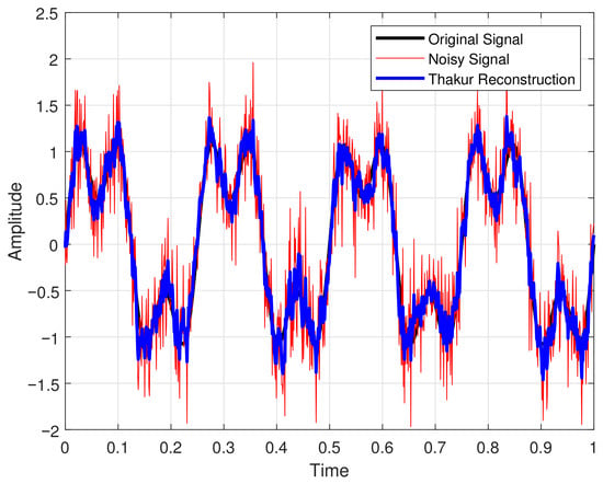
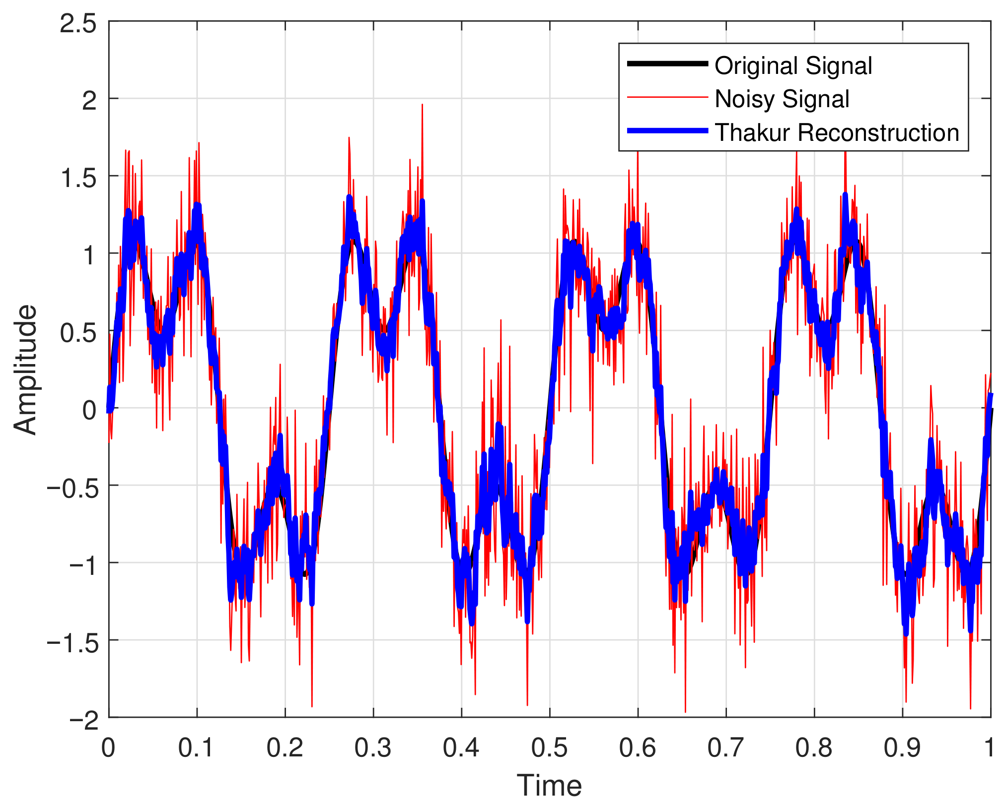
Figure 4 displays the original signal, the noisy observation, and the signal reconstructed by the Thakur iteration. The recovered signal captures the main pattern of the original waveform, but some differences between the reconstructed and exact signals can still be observed.
Figure 4.
Signal reconstruction using Thakur iteration.
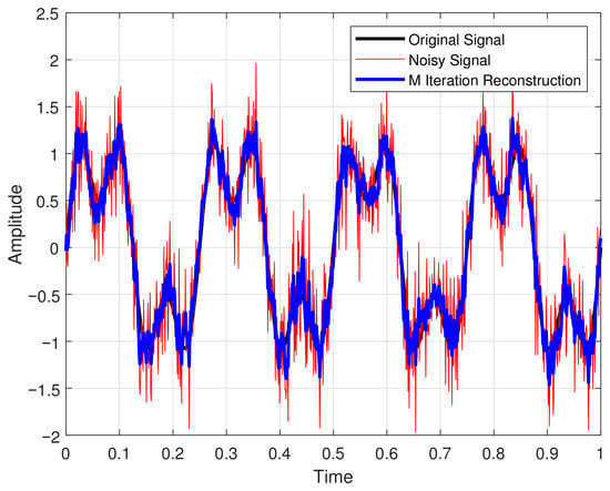
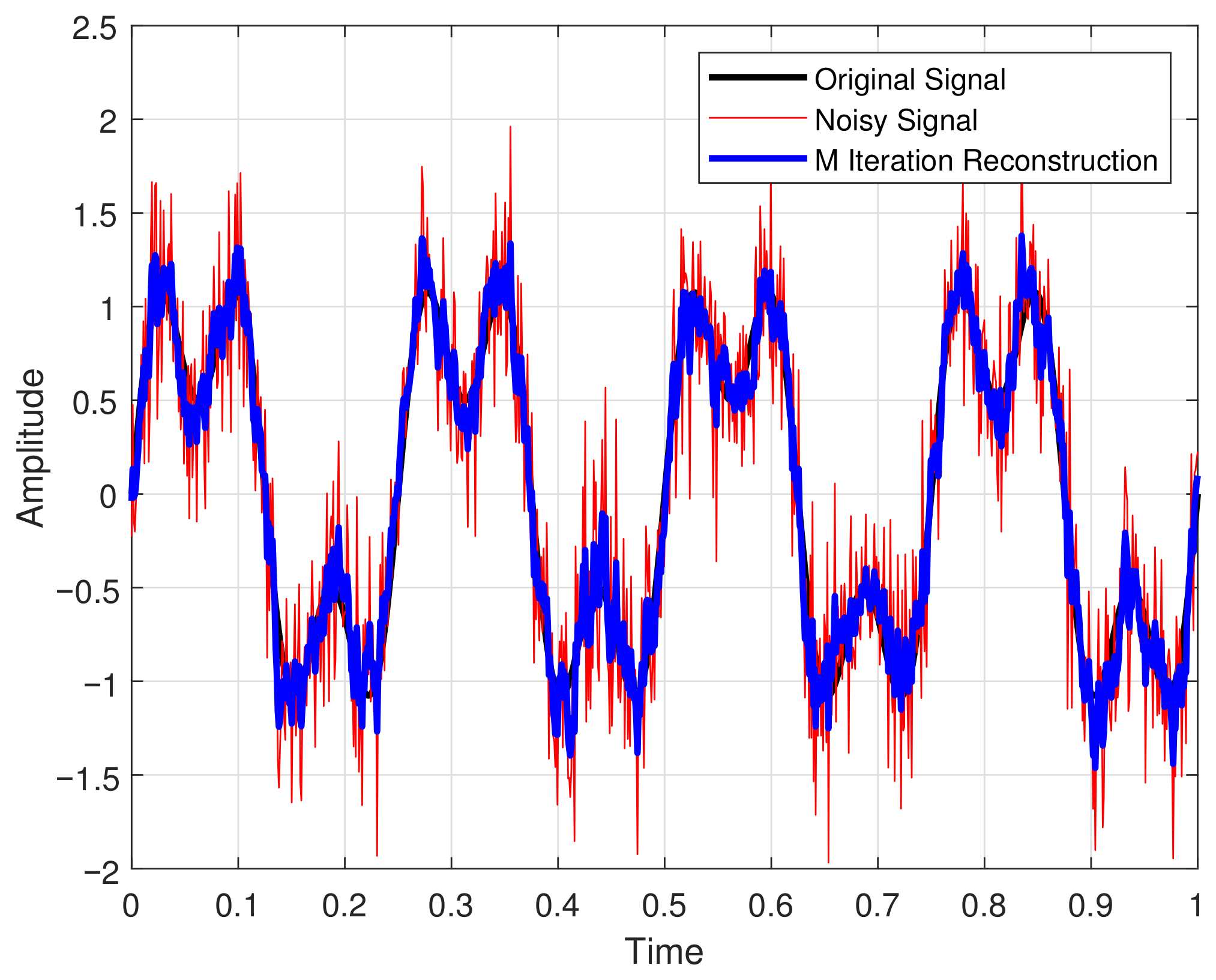
Figure 5 illustrates the reconstruction obtained using the M iteration. This method provides a smoother approximation than the Thakur iteration; however, certain noise-related irregularities remain visible in the reconstructed signal.
Figure 5.
Signal reconstruction using M-iteration.
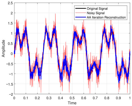
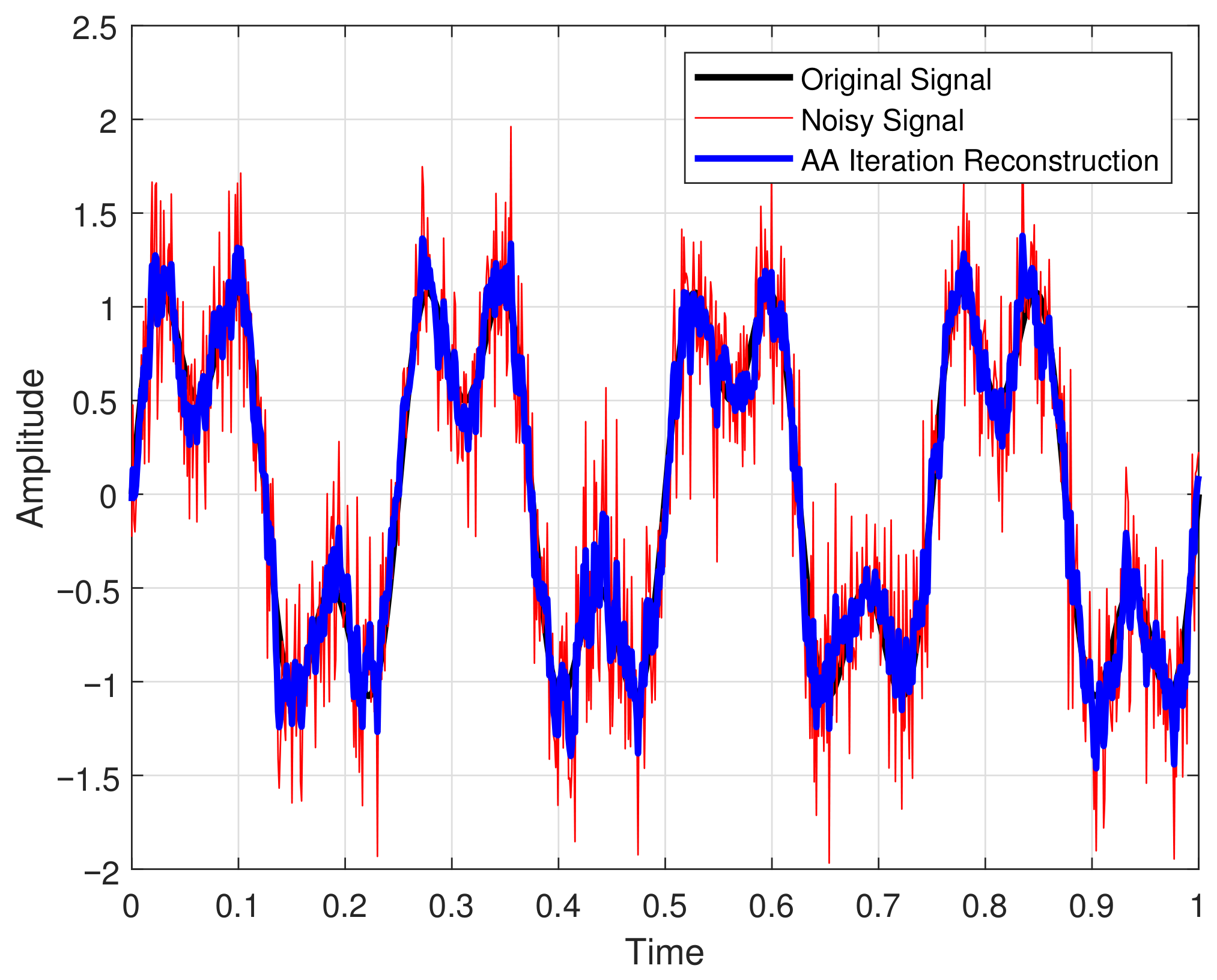
The reconstruction produced by the AA iteration is shown in Figure 6. The obtained result is closer to the original signal and exhibits better stability than the reconstructions generated by the previous iterative schemes.
Figure 6.
Signal reconstruction using AA-iteration.
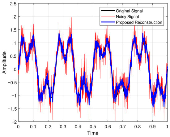
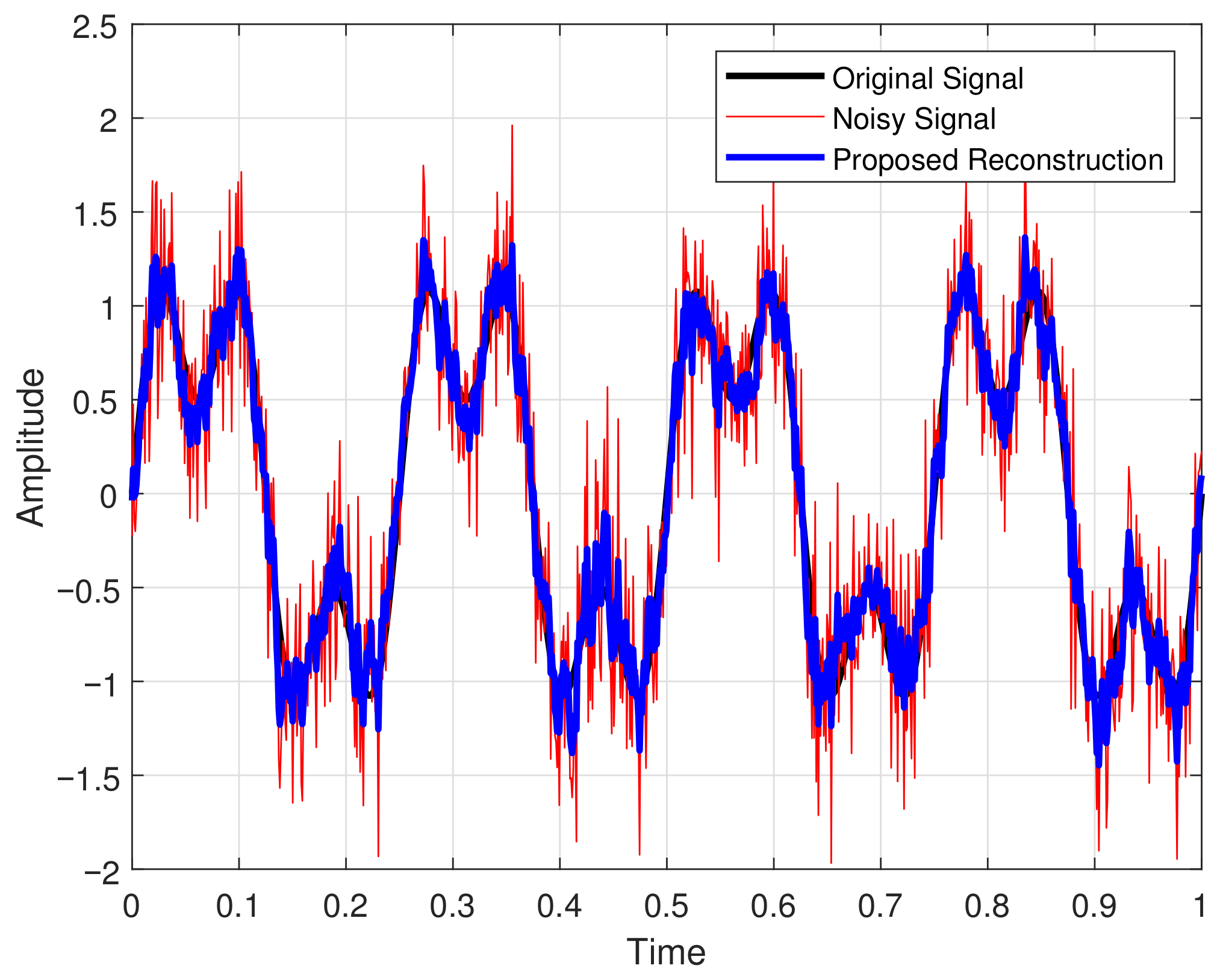
Figure 7 presents the signal recovered by the proposed inertial viscosity algorithm. The reconstructed waveform closely matches the original signal and effectively reduces the impact of noise. The inertial and viscosity terms contribute to a more stable and reliable reconstruction process.
Figure 7.
Signal reconstruction using proposed algorithm.
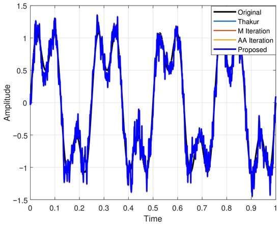
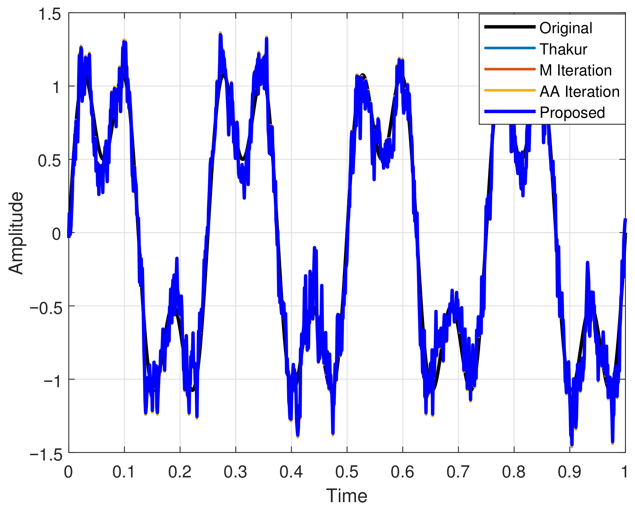
A visual comparison of all reconstructed signals is provided in Figure 8. Among the considered methods, the proposed algorithm yields a reconstruction that most closely resembles the original signal.
Figure 8.
Comparison of reconstruction schemes.
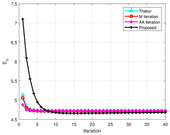
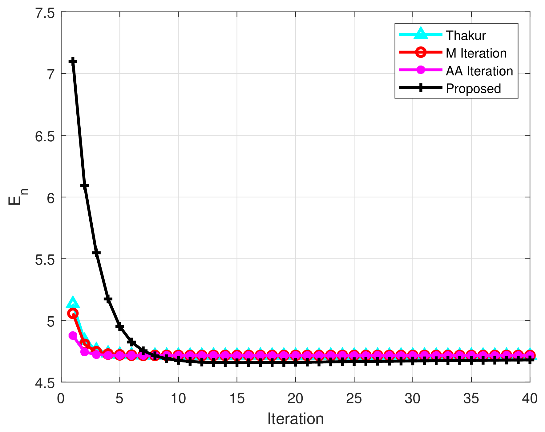
Figure 9 shows the error curves corresponding to the different iterative methods. While each algorithm converges, the proposed approach reduces the approximation error more rapidly, suggesting a faster convergence rate toward the fixed point of the operator S.
Figure 9.
Comparison of approximation errors.
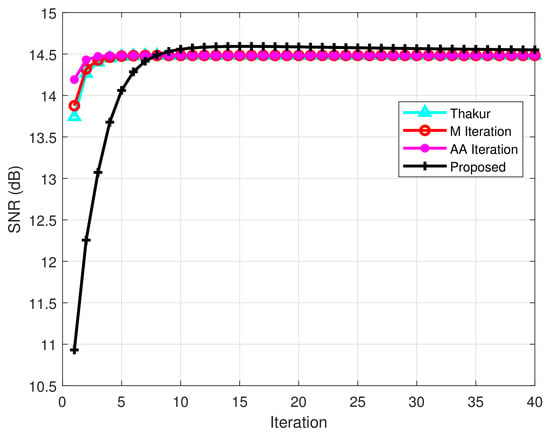
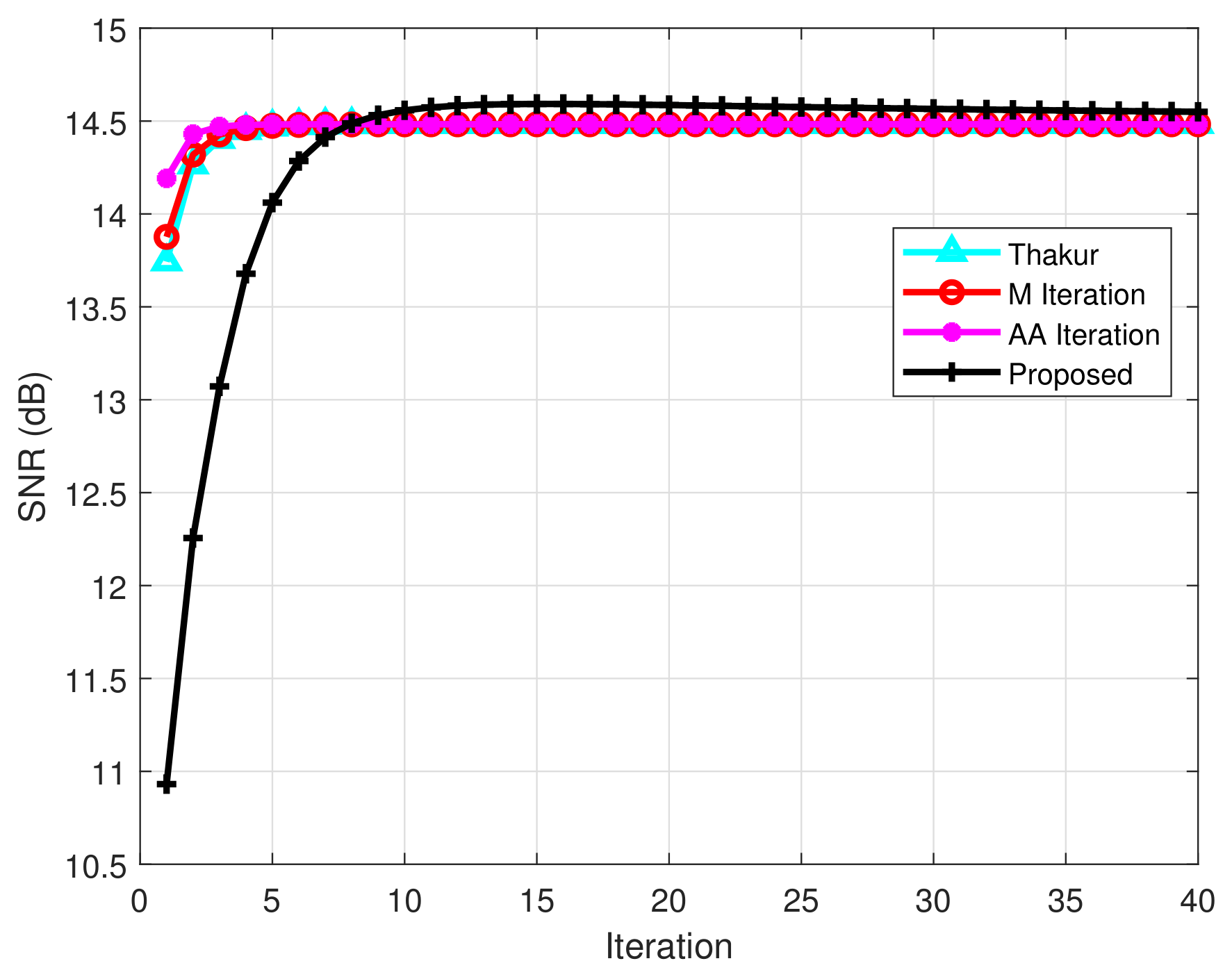
The variation of the signal-to-noise ratio is illustrated in Figure 10. The proposed method achieves higher SNR values with fewer iterations, indicating improved denoising performance and enhanced computational stability.
Figure 10.
Comparison of signal-to-noise ratios.
The results reported in Table 1 demonstrate the effectiveness of incorporating inertial and viscosity mechanisms into the iterative process. The proposed method not only converges quickly but also provides superior noise suppression, making it a suitable choice for signal reconstruction and denoising problems.
Table 1.
Comparison of errors and SNR values.
Convergence Rate Analysis
To further assess the numerical performance of the proposed inertial viscosity algorithm, we provide a quantitative comparison of its convergence behavior with the Thakur, M-iteration, and AA-iteration schemes. In addition to the approximation error curves presented in Figure 9, we consider the error reduction ratio
where . A smaller value of indicates a greater reduction in the approximation error from one iteration to the next and hence reflects faster numerical convergence.
The numerical results reported in Table 1 show that the proposed algorithm exhibits a faster reduction in the approximation error after the initial iterations. For instance, at the eighth iteration, the approximation error of the proposed method is 4.7133, whereas the corresponding errors for the Thakur, M, and AA iterations are 4.7169, 4.7165, and 4.7162, respectively. At the tenth iteration, the proposed method further reduces the error to 4.6755, while the corresponding errors of the Thakur, M, and AA methods remain close to 4.7163, 4.7162, and 4.7161, respectively. The proposed method continues to reduce the approximation error and attains a value of approximately 4.6571 at the fifteenth iteration. These observations are also consistent with Figure 9, where the error curve of the proposed method decreases more rapidly than those of the other considered schemes.
The above comparison indicates that the inertial and viscosity terms incorporated in the proposed algorithm can improve the numerical convergence behavior. Although the proposed scheme requires additional computational operations at each iteration because of its inertial and viscosity components, its faster reduction of the approximation error provides a useful computational advantage in terms of convergence behavior. Note that a detailed computational cost analysis involving CPU time, memory consumption, and implementation-dependent operation counts is not included in the present study. Such measurements may depend on the specific hardware, software environment, and implementation of each iterative scheme. Nevertheless, the iteration-wise error and SNR comparisons presented in Table 1 and Figure 9 and Figure 10 provide a direct numerical assessment of the convergence performance of the proposed method. A detailed implementation level computational cost comparison is left for future investigation.
4.2. Application to Virus Transmission Model
Now, we shall study an application of proposed iterative scheme in mathematical modeling which gives the transmission of a viral disease. The model takes into account the periodic variation in the infection rate and is represented by a nonlinear integral equation. Such models are commonly used to investigate the evolution of infectious diseases whose transmission patterns change periodically over time.
Consider the integral equation
where represent the number of infected individuals at the time , represents rate of newly infected cases, and is the infectious period during which an infected individual can transmit the disease. We assume that which means that no new infections occur when there are no infected individuals.
If is Banach space of continuous -periodic functions on , equipped with the norm given by Under this norm, is a uniformly convex Banach space. Let denote the cone of positive functions in . Define an operator by
The following result helps to solve (55).
Theorem 2.
Consider the following:
- (i)
- is continuous map.
- (ii)
- for any and .
- (iii)
- (iv)
- for all .
Then Equation (55) admits the solution. Moreover, the proposed iterative method approximate the solution of this particular problem.
Proof.
Note that.
As , we have
Therefore, is nonexpansive.
As is the closed bounded and convex subset of a uniformly convex Banach space , the operator possesses a fixed point in . Consequently, (55) has a solution. The convergence of the proposed iterative process then follows from the main convergence theorem proved earlier. □
4.3. Application to Constrained Optimization Problem
Constrained optimization problems appear in many areas of mathematics, engineering, and the applied sciences. In particular, they play a significant role in image restoration, signal processing, machine learning, and resource allocation problems. The main objective of these problems is to determine an optimal point that minimizes a given function while satisfying a collection of constraints represented by a feasible set. In many practical situations, these constraints arise from physical limitations, design requirements, or available data.
Let be convex and closed subset. Assume that is a -inverse strongly monotone (-ism) operator for some . In this case, the map is nonexpansive whenever Furthermore, the gradient of a convex differentiable function which is continuous operator with Lipschitz constant ℓ is -cocoercive (equivalently, -ism under the adopted convention). This property allows optimization problems to be studied through fixed point techniques associated with nonexpansive mappings.
We now present an iterative scheme to solve constrained convex minimization problem. Note that we take in our proposed algorithm, then generated sequence remains in the feasible set and converges to a minimizer of the objective function.
Theorem 3.
Let be a nonempty closed convex subset of a Hilbert space , and let be a convex and differentiable function on an open set , and h is contraction. Assume that the gradient operator is Lipschitz continuous on U with Lipschitz constant ℓ, and let Assume has a minimizer over
, define the sequence as
where , , , and are sequences in . Then converges to minimizer of over the set .
4.4. Application to Variational Inequality Problem
Variational inequality problems (VIPs) is an important class of nonlinear problems in applied mathematics. They provide a powerful mathematical framework to study many nonlinear models arising in science and engineering. In particular, VIPs are closely related to boundary value problems associated with elliptic and parabolic partial differential equations. A variational inequality establishes a relationship between an operator and the elements of a feasible set. Due to their rich theoretical structure and practical relevance, VIPs have attracted significant attention from researchers over the past several decades.
These problems have numerous applications in optimization, equilibrium theory, image restoration, signal processing, optimal control, economics, and other areas of applied sciences (see, for example, refs. [21,22,23,24,25]).
Let be the nonlinear operator. Following [26], the VIP, denoted by , is find such that
The solution of is represented with . It is worth mentioning that VIPs are closely connected with several other mathematical models, including complementarity problems, convex optimization problems, and the problem of finding a zero of an operator. In particular, determining a point satisfying can be viewed as a special case related to variational inequalities.
An important feature of VIPs is that they can be reformulated as fixed point problems. More precisely, a point solves iff where and denotes the metric projection onto . By defining the VIP is transformed into the problem of finding a fixed point of the operator .
Furthermore, suppose that is ℓ-Lipschitz continuous and -strongly monotone. Then becomes a contraction whenever Consequently, by the Banach contraction principle, the solution set reduces to a singleton, that is, and the sequence of Picard iteration converges to the unique solution . When the associated mappings are nonexpansive rather than contractive, the VIP can still be studied through an equivalent fixed point formulation. In the case of nonexpansive mappings, we need to use some other iteration, for this application, we take in our proposed algorithm and present in the subsequent theorem.
Theorem 4.
If is as defined above and is ℓ-Lipschitz continuous and ς-strongly monotone operator and h is contraction. Then define by
converges a solution .
4.5. Application to Split Feasibility Problem
The split feasibility problem (SFP), introduced by [27], it is an important problem in nonlinear analysis and optimization. Over the years, it has received considerable attention due to its usefulness in both theoretical studies and practical applications. This SFP used in different problems such as: image reconstruction, signal recovery, pattern recognition and medical imaging. For further developments and applications, we refer the reader to [28,29,30,31,32].
Fixed point theory plays a central role in the study of the SFP since many solution methods are based on reformulating the problem as an equivalent fixed point equation involving nonexpansive operators.
Let , and , and assume is a bounded linear operator. Now, the solution set of SFP is denoted by , that is, find a point such that
It is known SFP can be expressed in terms of a fixed point equation. More precisely, a point r solves if and only if
where and denote the metric projections onto and , respectively, is adjoint of , . Moreover, the operator is nonexpansive.
Recall that an operator T is averaged if we can represented as here with S is nonexpansive.
Now define the function by
The corresponding optimization problem is According to [33], the gradient of g is given by Since the operator is nonexpansive, it follows that is ℓ-Lipschitz continuous with provided that . Hence, is -inverse strongly monotone. Therefore, for every the operator is averaged.
Since the composition of an averaged operator with a projection remains averaged, the operator is also averaged.
Then the set of solutions of is same as fixed point set of the operator T. This observation allows us to employ iterative fixed point techniques to approximate solutions of the split feasibility problem.
The following theorem provides a convergence result for the proposed iterative method in which we set and given in the theorem below:
Theorem 5.
If and g given as above, h is contraction, and the sequence be generated by
Then converges to a solution of .
5. Conclusions
This research developed an inertial viscosity type iterative scheme for approximating solutions of equilibrium fixed point problems associated with nonexpansive mappings. Under suitable assumptions, strong convergence of the proposed method was established. The numerical experiments demonstrate that the inertial mechanism can improve the convergence behavior compared with several existing iterative schemes. The results also highlight the influence of initial guesses and parameter selection on the convergence behavior, which confirm the efficiency of our approach across different test cases. The proposed approach was further applied to signal reconstruction, viral disease transmission modeling, constrained optimization, and split feasibility problems, illustrating its applicability to several classes of nonlinear problems.
Author Contributions
M.A. and M.W.A. contributed to the conceptualization and methodology of the study. M.A. developed the theoretical framework and contributed to the analysis of the convergence results. M.W.A. contributed to the development of the iterative scheme, numerical experiments, interpretation of the results, and manuscript preparation. All authors have read and agreed to the published version of the manuscript.
Funding
This article has been supported by Faculty of Engineering and the Built Environment, University of Johannesburg, South Africa.
Data Availability Statement
No external datasets were required or used in this study. By using the MATLAB software, all numerical results were generated from the mathematical models, parameter values, and computational procedures reported in the manuscript.
Acknowledgments
The second author is grateful to the University of Johannesburg, for providing the postdoctoral fellowship.
Conflicts of Interest
The authors report no competing interests.
References
- Barbagallo, A. Existence and regularity of solutions to nonlinear degenerate evolutionary variational inequalities with applications to dynamic network equilibrium problems. Appl. Math. Comput. 2009, 208, 1–13. [Google Scholar] [CrossRef] [Scilit]
- Dafermos, S.; Nagurney, A. A network formulation of market equilibrium problems and variational inequalities. Oper. Res. Lett. 1984, 3, 247–250. [Google Scholar] [CrossRef] [Scilit]
- He, R. Coincidence theorem and existence theorems of solutions for a system of Ky Fan type minimax inequalities in FC-spaces. Adv. Fixed Point Theory 2012, 2, 47–57. [Google Scholar]
- Qin, X.; Cho, S.Y.; Kang, S.M. Strong convergence of shrinking projection methods for quasi-ϕ-nonexpansive mappings and equilibrium problems. J. Comput. Appl. Math. 2010, 234, 750–760. [Google Scholar] [CrossRef] [Scilit]
- Mann, W.R. Mean value methods in iteration. Proc. Amer. Math. Soc. 1953, 4, 506–510. [Google Scholar] [CrossRef] [Scilit]
- Ishikawa, S. Fixed points by a new iteration method. Proc. Amer. Math. Soc. 1974, 44, 147–150. [Google Scholar] [CrossRef] [Scilit]
- Noor, M.A. New approximation schemes for general variational inequalities. J. Math. Anal. Appl. 2000, 251, 217–229. [Google Scholar] [CrossRef] [Scilit]
- Agarwal, R.P.; Regan, D.O.; Sahu, D.R. Iterative construction of fixed points of nearly asymptotically nonexpansive mappings. J. Nonlinear Convex Anal. 2007, 8, 61. [Google Scholar]
- Abbas, M.; Nazir, T. Some new faster iteration process applied to constrained minimization and feasibility problems. Mat. Vesn. 2014, 66, 223–234. [Google Scholar]
- Thakur, B.S.; Thakur, D.; Postolache, M. A new iteration scheme for approximating fixed points of nonexpansive mappings. Filomat 2016, 30, 2711–2720. [Google Scholar] [CrossRef] [Scilit]
- Ullah, K.; Arshad, M. Numerical reckoning of fixed points for Suzuki’s generalized nonexpansive mappings via new iteration process. Filomat 2018, 32, 187–196. [Google Scholar] [CrossRef] [Scilit]
- Abbas, M.; Asghar, M.W.; De la Sen, M. Approximation of the solution of delay fractional differential equation using AA-iterative scheme. Mathematics 2022, 10, 273. [Google Scholar] [CrossRef] [Scilit]
- Sharma, S.; Chandok, S. Iterative methods to approximate the solution of optimal problems with applications to nonlinear models. Math. Methods Appl. Sci. 2025, 48, 13142–13154. [Google Scholar] [CrossRef] [Scilit]
- Alakoya, T.O.; Mewomo, O.T. Viscosity S-iteration method with inertial technique and self-adaptive step size for split variational inclusion, equilibrium and fixed point problems. Comp. Appl. Math. 2022, 41, 39. [Google Scholar] [CrossRef] [Scilit]
- Zhao, J.; Liang, Y.; Liu, Y.; Cho, Y.J. Split equilibrium, variational inequality and fixed point problems for multi-valued mappings in Hilbert spaces. Appl. Comput. Math 2018, 17, 271–283. [Google Scholar]
- Chuang, C.-S. Strong convergence theorems for the split variational inclusion problem in Hilbert spaces. Fixed Point Theory Appl. 2013, 2013, 350. [Google Scholar] [CrossRef] [Scilit][Green Version]
- Osilike, M.O.; Igbokwe, D.I. Weak and strong convergence theorems for fixed points of pseudocontractions and solutions of monotone type operator equations. Comput. Math. Appl. 2000, 40, 559–567. [Google Scholar] [CrossRef] [Scilit]
- Maingé, P.-E. Approximation methods for common fixed points of nonexpansive mappings in Hilbert spaces. J. Math. Anal. Appl. 2007, 325, 469–479. [Google Scholar] [CrossRef] [Scilit]
- Saejung, S.; Yotkaew, P. Approximation of zeros of inverse strongly monotone operators in Banach spaces. Nonlinear Anal. 2012, 75, 742–750. [Google Scholar] [CrossRef] [Scilit]
- Ma, Z.; Wang, L.; Chang, S.-S.; Duan, W. Convergence theorems for split equality mixed equilibrium problems with applications. Fixed Point Theory Appl. 2015, 2015, 31. [Google Scholar] [CrossRef] [Scilit]
- Ceng, L.C. A modified inertial subgradient extragradient method for solving pseudomonotone variational inequalities and common fixed point problems. Fixed Point Theory 2020, 21, 93–108. [Google Scholar] [CrossRef] [Scilit]
- Ceng, L.C. A subgradient-extragradient method for bilevel equilibrium problems with the constraints of variational inclusion systems and fixed point problems. Commun. Optim. Theory 2021, 2021, 4. [Google Scholar] [CrossRef]
- Liu, L.; Cho, S.Y.; Yao, J.C. Convergence analysis of an inertial Tsengs extragradient algorithm for solving pseudomonotone variational inequalities and applications. J. Nonlinear Var. Anal. 2021, 5, 627–644. [Google Scholar] [CrossRef] [Scilit]
- Liu, L.; Qin, X. Strong convergence theorems for solving pseudo-monotone variational inequality problems and applications. Optimization 2022, 71, 3603–3626. [Google Scholar] [CrossRef] [Scilit]
- Liu, L.; Yao, J.C. Iterative methods for solving variational inequality problems with a double hierarchical structure in Hilbert spaces. Optimization 2023, 72, 2195–2216. [Google Scholar] [CrossRef] [Scilit]
- Kinderlehrer, D.; Stampacchia, G. An Introduction to Variational Inequalities and Their Applications; SIAM: Philadelphia, PA, USA, 2000. [Google Scholar]
- Censor, Y.; Elfving, T. A multiprojection algorithm using Bregman projections in a product space. Num. Algo. 1994, 8, 221–239. [Google Scholar] [CrossRef] [Scilit]
- Bin Dehaish, B.A. A regularization projection algorithm for various problems with nonlinear mappings in Hilbert spaces. J. Inequal. Appl. 2015, 2015, 51. [Google Scholar] [CrossRef] [Scilit]
- Lu, T.; Zhao, L.; He, H. A multi-view on the CQ algorithm for split feasibility problems: From optimization lens. J. Appl. Numer. Optim. 2020, 2, 387–399. [Google Scholar] [CrossRef] [Scilit]
- Osilike, M.O.; Chima, E.E. Mixed equilibrium and multiple-set split feasibility problems for asymptotically k-strictly pseudononspreading mappings. Commun. Optim. Theory 2020, 2020, 14. [Google Scholar] [CrossRef]
- Xu, T.; Zhang, Z.; Shi, L. Strong convergence of an explicit extragradient-like method for a split feasibility problem. J. Nonlinear Funct. Anal. 2022, 2022, 16. [Google Scholar] [CrossRef] [Scilit]
- Moudafi, A. Byrne’s extended CQ-algorithms in the light of Moreau Yosida regularization. Appl. Set Valued Anal. Optim. 2021, 3, 21–26. [Google Scholar] [CrossRef] [Scilit]
- Aubin, J.P.; Cellina, A. Differential inclusions with maximal monotone maps. In Differential Inclusions: Set-Valued Maps and Viability Theory; Springer: Berlin/Heidelberg, Germany, 1984; pp. 139–171. [Google Scholar]

Disclaimer/Publisher’s Note: The statements, opinions and data contained in all publications are solely those of the individual author(s) and contributor(s) and not of MDPI and/or the editor(s). MDPI and/or the editor(s) disclaim responsibility for any injury to people or property resulting from any ideas, methods, instructions or products referred to in the content. |
© 2026 by the authors. Licensee MDPI, Basel, Switzerland. This article is an open access article distributed under the terms and conditions of the Creative Commons Attribution (CC BY) license.